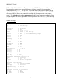
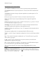
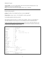
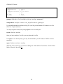
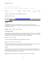
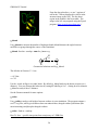
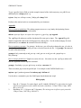
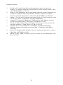
1
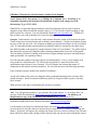
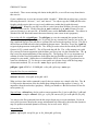
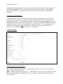
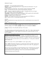
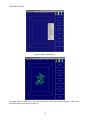
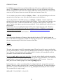
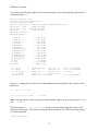
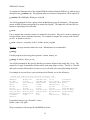
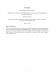
GROMACS Tutorial
GROMACS Introductory Tutorial
Gromacs ver 4.0
Author:
John E. Kerrigan, Ph.D.
Associate Director, Bioinformatics
The Cancer Institute of NJ
195 Little Albany Street
New Brunswick, NJ 08903
Phone:
Fax:
Email:
(732) 235-4473
(732) 235-6267
[email protected]
1
GROMACS Tutorial
GROMACS Tutorial for Solvation Study of Spider Toxin Peptide.
Yu, H., Rosen, M. K., Saccomano, N. A., Phillips, D., Volkmann, R. A., Schreiber, S. L.:
Sequential assignment and structure determination of spider toxin omega-Aga-IVB.
Biochemistry 32 pp. 13123 (1993)
GROMACS is a high-end, high performance research tool designed for the study of protein
dynamics using classical molecular dynamics theory. [1] This versatile software package is Gnu
public license free software. You may download it from http://www.gromacs.org . GROMACS
runs on linux, unix, and on Windows (a recent development).
Synopsis. In this tutorial, you will study a toxin isolated from the venom of the funnel web spider.
Venom toxins have been used in the past to identify cation channels. Calcium ion channels regulate
the entry of this ion into cells. Nerve signals are highly governed by the balance of ions in neuronal
cells. It is hypothesized that exposed positively charged residues in venoms like the spider toxin
here bind favorably to the negatively charged entrance of the cell’s ion channel. The spider toxin in
this tutorial has its positively charged residues pointing predominantly to one side of the peptide.
The ion channel is blocked, resulting in blocked nerve signal leading to paralysis and ultimately to
death (presumably via respiratory failure).
We will study this peptide toxin using explicit solvation dynamics. First, we will compare an in
vacuo model to a solvated model. We will solvate the peptide in a water box followed by
equilibration using Newton’s laws of motion. We will compare and contrast the impact of
counterions in the explicit solvation simulation. We will seek answers to the following questions:
Is the secondary structure stable to the dynamics conditions?
Are the side chains of the positively charged residues predominantly displaced to one side of the
peptide structure? Do the counterions hold these positively charged residues in place or do they
move around?
What role does water play in maintaining the structure of proteins?
Note: You will generate gromacs (*.gro) structure files in this tutorial. To view these files, you
must use VMD (Download from: http://www.ks.uiuc.edu/Research/vmd/ ). In addition, you
should obtain a copy of the GROMACS user manual at http://www.gromacs.org .
Download 1OMB.PDB from the Protein Data Bank (http://www.rcsb.org/pdb/).
It is advisable to use DeepView (Download DeepView from http://www.expasy.ch/spdbv/ ) to
preview the file if you know that your structure may be disordered (i.e. residues with missing side
chains). DeepView will replace any missing side chains (However, beware as Deep View will mark
those rebuilt side chains with a strange control character that can only be removed manually using a
2
GROMACS Tutorial
text editor!). There are no missing side chains in this pdb file, so we will not worry about that in
this exercise.
Create a subdirectory in your unix account called “fwspider”. Within this new directory, create the
following directories: “invacuo”, “wet”, and “ionwet”. Use sftp to copy the 1OMB.pdb file to the
fwspider subdirectories (place a copy in each subdirectory within the fwspider directory).
(IMPORTANT! Whenever you sftp a text file to a unix system from Windows, be sure to convert
the file to a unix text file. Do this using the to_unix command (e.g. to_unix filename filename
converts filename to a unix text file. In RedHat Linux, use the dos2unix command. Text editors in
Windows like MS Word add control characters that may cause errors in unix programs.)
Process the pdb file with pdb2gmx. The pdb2gmx (to view the command line options for this
command just type pdb2gmx –h; In fact, to get help for any command in Gromacs just use the –h
flag) command converts your pdb file to a gromacs file and writes the topology for you. This file is
derived from an NMR structure which contains hydrogen atoms. Therefore, we use the –ignh flag
to ignore hydrogen atoms in the pdb file. The –ff flag is used to select the forcefield (G43a1 is the
Gromos 96 FF, a united atom FF). The –f flag reads the pdb file. The –o flag outputs a new pdb
file (various file formats supported) with the name you have given it in the command line. The –p
flag is used for output and naming of the topology file. The topology file is very important as it
contains all of the forcefield parameters (based upon the forcefield that you select in the initial
prompt) for your model. Studies have revealed that the SPC/E water model [2] performs best in
water box simulations. [3] Use the spce water model as it is better for use with the long-range
electrostatics methods. So, we use the –water flag to specify this model.
pdb2gmx –ignh –ff G43a1 –f 1OMB.pdb –o fws.pdb –p fws.top –water spce
Setup the Box for your simulations
editconf -bt cubic –f fws.pdb –o fws.pdb –d 0.9
What you have done in this command is specify that you want to use a simple cubic box. The –d
0.9 flag sets the dimensions of the box based upon setting the box edge approx 0.9 nm (i.e. 9.0
angstroms) from the molecule(s) periphery. Ideally you should set –d at no less than 0.85 nm for
most systems. [4]
[Special Note: editconf may also be used to convert gromacs files (*.gro) to pdb files (*.pdb) and
vice versa. For example: editconf –f file.gro –o file.pdb converts file.gro to the pdb file file.pdb]
You may use the files generated from the this step to begin your in vacuo simulation. For the in
vacuo work just move ahead to the energy minimization step followed by the molecular dynamics
step (No position restrained dynamics necessary for in vacuo work. Why?).
Solvate the Box
genbox –cp fws.pdb –cs spc216.gro –o fws_b4em.pdb –p fws.top
3
GROMACS Tutorial
The genbox command generates the water box based upon the dimensions/box type that you had
specified using editconf. In the command above, we specify the spc water box. The genbox
program will add the correct number of water molecules needed to solvate your box of given
dimensions.
Setup the energy minimization.
Use the em.mdp file. Gromacs uses special *.mdp files to setup the parameters for every type of
calculation that it performs. Look into the contents of this file. It specifies a steepest descents
minimization to remove bad van der Waals contacts. Edit the file and change nsteps to 400. If the
minimization fails to converge, re-submit with nsteps = 500. (The minimization should converge in
less than 400 steps; however, different platforms respond differently.) To re-submit the job, you
will need to re-run grompp. (Note: the path to the c pre-processor may be different on your
machine. Use the which command to locate [i.e. which cpp]!)
Content of em.mdp:
title
= FWS
cpp
= /usr/bin/cpp ; the c pre-processor
define
= -DFLEXIBLE
constraints
= none
integrator
= steep
dt
= 0.002
; ps !
nsteps
= 400
nstlist
= 10
ns_type
= grid
rlist
= 1.0
coulombtype
= PME
rcoulomb
= 1.0
vdwtype
= cut-off
rvdw
= 1.4
fourierspacing
= 0.12
fourier_nx
= 0
fourier_ny
= 0
fourier_nz
= 0
pme_order
= 4
ewald_rtol
= 1e-5
optimize_fft
= yes
;
;
Energy minimizing stuff
;
emtol
= 1000.0
emstep
= 0.01
Important aspects of the em.mdp file:
title – The title can be any given text description (limit 64 characters; keep it short and simple!)
cpp – location of the pre-processor
define – defines to pass to the pre-processor. –DFLEXIBLE will tell grompp to include the flexible
SPC water model instead of the rigid SPC into your topology. This allows steepest descents to
minimize further.
4
GROMACS Tutorial
constraints – sets any constraints used in the model.
integrator – steep tells grompp that this run is a steepest descents minimization. Use cg for
conjugate gradient.
dt – not necessary for minimization. Only needed for dynamics integrators (like md).
nsteps – In minimization runs, this is just the maximum number of iterations.
nstlist – frequency to update the neighbor list. nstlist = 10 (updates the list every 10 steps).
rlist – cut-off distance for short-range neighbor list.
coulombtype – tells gromacs how to model electrostatics. PME is particle mesh ewald method
(please see the Gromacs user manual for more information).
rcoulomb – distance for the coulomb cut-off
vdwtype – tells Gromacs how to treat van der Waals interactions (cut-off, Shift, etc.)
rvdw – distance for the LJ or Buckingham potential cut-off
EM Stuff
emtol – the minimization converges when the max force is smaller than this value (in units of kJ
mol–1 nm–1)
emstep – initial step size (in nm).
Now process the files with grompp. grompp is the pre-processor program (the gromacs preprocessor “grompp” Get it! Sigh!). grompp will setup your run for input into mdrun.
grompp –f em.mdp –c fws_b4em.pdb –p fws.top –o fws_em.tpr
The –f flag in grompp is used to input the parameter file (*.mdp). The –c flag is used to input the
coordinate file (the pdb file, *.pdb); -p inputs the topology and –o outputs the input file (*.tpr)
needed for mdrun.
Using genion and the tpr file to add ions. You may use the tpr file generated here to add
counterions to your model to neutralize any net charge. Our model has a net charge of + 2.00.
Therefore, we want to add two chloride ions. Copy the fws_em.tpr file that you used for your
explicit solvated model to your “ionwet” subdirectory. In addition, copy your fws.top and posre.itp
files from your explicit solvation model to your ionwet subdirectory. Use the genion command to
add the chloride ions.
genion –s fws_em.tpr –o fws_ion.pdb –nname CL- –nn 2 –g fws_ion.log
Where –nname is the negative ion name (CL- for the Gromos G43a1 force field; see the ions.itp
file for specifics wrt force field), -nn is the number of negative ions to add. The –g flag gives a
name to the output log for genion.
When you process this command, you will be prompted to provide a continuous group of solvent
molecules, which should be Group 12 (SOL). Type 12 then <enter>. You will notice that two
solvent molecules have been replaced by Cl ions. Now you must make the following
additions/corrections to your fws.top file:
Add
5
GROMACS Tutorial
#include “ions.itp” (Note: This should be present by default already in version 3.2 & greater)
after the include statement for the force field. Subtract 2 from the total number of SOL molecules
and add a line for 2 Cl molecules in the [ molecules ] section at the end of the file. You will also
need to modify the temperature coupling scheme for your pr_md.mdp and md.mdp files.
Now, you will use fws_ion.pdb in place of fws_b4em.pdb for generating the actual input tpr using
grompp for energy minimization.
Temperature coupling scheme for the pr_md.mdp and md.mdp files after adding chloride ions.
; Berendsen temperature coupling using vel rescaling is on
Tcoupl
= v-rescale
tau_t
= 0.1
0.1
tc_grps
= protein
non-protein
ref_t
= 300
300
Remember: If you added the chloride ions, you will need to run the grompp step again. First
remove the old fws_em.tpr file, then run the next grompp command below. We added chloride ions
in our model to neutralize the overall net charge of the model.
grompp –f em.mdp –c fws_ion.pdb –p fws.top –o fws_em.tpr
Run the energy minimization in background (Use the ampersand & at the end of the command).
nohup mdrun –v –s fws_em.tpr –o fws_em.trr –c fws_b4pr.pdb –e em.edr –g em.log &
Use the tail command to check on the progress of the minimization.
tail –15 em.log
When the minimization is complete, you should see the following summary in your log file
indicating that steepest descents converged. Use tail -50 em.log
Steepest Descents
Potential Energy
Maximum force
Norm of force
converged to Fmax < 1000 in 245 steps
= -2.0551497e+05
= 8.9138922e+02 on atom 106
= 5.0448242e+03
Setup the position-restrained molecular dynamics. What is position-restrained MD? You are
restraining (or partially freezing, if you will) the atom positions of the macromolecule while letting
the solvent move in the simulation. This is done to “soak” the water molecules into the
macromolecule. The relaxation time of water is ~ 10 ps. Therefore, we need to do dynamics in
excess of 10 ps for position-restrained work. This example uses a 20.0 ps time scale (at least an
order of magnitude greater. Larger models (large proteins/lipids) may require longer preequilibration periods of 50 or 100 ps or more. The settings below will work well for the Gromacs
force field. Consult the Gromacs manual for optimal settings for other force fields (e.g. the
GROMOS 96 force field nstlist = 10 and rvdw = 1.4 are recommended). Under coulombtype,
6
GROMACS Tutorial
PME stands for “Particle Mesh Ewald” electrostatics. [5, 6] PME is the best method for computing
long-range electrostatics (gives more reliable energy estimates especially for systems where
counterions like Na+, Cl-, Ca 2+ , etc. are used). Due to the nature of this particular protein having
exposed charged residues with a net +2 charge to the system, it is beneficial for us to use PME. It is
even more beneficial for us to use counterions to balance the charge and set the system to net
neutral. The all-bonds option under constraints applies the Linear Constraint algorithm for fixing
all bond lengths in the system (important to use this option when dt > 0.001 ps). [7] Study the mdp
file below.
Content of pr.mdp.
title
= FWS
warnings
= 10
cpp
= /usr/bin/cpp
define
= -DPOSRES
constraints
= all-bonds
integrator
= md
dt
= 0.002 ; ps !
nsteps
= 10000 ; total 20.0 ps.
nstcomm
= 1
nstxout
= 250
; collect data every 0.5 ps
nstvout
= 1000
nstfout
= 0
nstlog
= 10
nstenergy
= 10
nstlist
= 10
ns_type
= grid
rlist
= 1.0
coulombtype
= PME
rcoulomb
= 1.0
vdwtype
= cut-off
rvdw
= 1.4
fourierspacing
= 0.12
fourier_nx
= 0
fourier_ny
= 0
fourier_nz
= 0
pme_order
= 4
ewald_rtol
= 1e-5
optimize_fft
= yes
; Berendsen temperature coupling is on
Tcoupl
= v-rescale
tau_t
= 0.1
0.1
tc-grps
= protein non-protein
ref_t
= 300
300
; Pressure coupling is on
Pcoupl
= parrinello-rahman
Pcoupltype
= isotropic
tau_p
= 0.5
compressibility
= 4.5e-5
ref_p
= 1.0
; Generate velocites is on at 300 K.
gen_vel
= yes
gen_temp
= 300.0
gen_seed
= 173529
7
GROMACS Tutorial
Important things to know about the mdp file.
The –DPOSRE in the define statement tells Gromacs to perform position restrained dynamics.
The constraints statement is as previously discussed. all-bonds sets the LINCS constraint for all
bonds. [7]
The integrator tells gromacs what type of dynamics algorithm to use (another option is “sd” for
stochastic dynamics).
dt is the time step (we have selected 2 fs; however, this must be entered in units of ps!).
nsteps is the number of steps to run (just multiply nsteps X dt to compute the length of the
simulation).
nstxout tells gromacs how often to collect a “snapshot” for the trajectory. (e.g. nstxout = 250 with
dt = 0.002 would collect a snapshot every 0.5 ps)
coulombtype selects the manner in which Gromacs computes electrostatic interactions between
atoms. (PME is particle mesh ewald; there are other options like cut-off).
rcoulomb and rvdw are the cutoffs (in nm; 1.0 nm = 10.0 angstroms) for the electrostatic and van
der Waals terms.
The temperature coupling section is very important and must be filled out correctly.
Tcoupl = v-rescale [8, 9] (type of temperature coupling where velocity is rescaled using a stochastic
term.)
tau_t = Time constant for temperature coupling (units = ps). You must list one per tc_grp in the
order in which tc_grps appear.
tc_grps = groups to couple to the thermostat (every atom or residue in your model must be
represented here by appropriate index groups).
ref_t = reference temperature for coupling (i.e. the temperature of your MD simulation in degrees
K). You must list one per tc_grp in the order in which tc_grps appear.
When you alter the temperature, don’t forget to change the gen_temp variable for velocity
generation.
pcoupl – is the Parrinello-Rahman barostat.
pcoupltype – isotropic means that the “box” will expand or contract evenly in all directions (x, y,
and z) in order to maintain the proper pressure. Note: Use semiisotropic for membrane simulations.
tau_p – time constant for coupling (in ps).
8
GROMACS Tutorial
compressibility – this is the compressibility of the solvent used in the simulation in bar–1 (the
setting above is for water at 300 K and 1 atm).
ref_p – the reference pressure for the coupling (in bar) (1 atm ~ 0.983 bar).
Pre-process the pr.mdp file.
grompp –f pr.mdp –c fws_b4pr.pdb –p fws.top –o pr.tpr –maxwarn 3
nohup mdrun –s pr.tpr –o pr.trr –c fws_b4md.pdb –e pr.edr –g pr.log &
Use the tail command to check the pr.log file.
The md.mdp parameter file looks very similar to the pr.mdp file. There are several differences.
The define statement is not necessary as we are not running as position restrained dynamics.
Content of md.mdp for explicit solvation (Special Note: For in vacuo, remove the entries for “sol”
in the temperature coupling section. For the simulation that includes the counterions, add an entry
for the ions in the temperature coupling section.)
title
= FWS
cpp
= /usr/bin/cpp
constraints
= all-bonds
integrator
= md
dt
= 0.002 ; ps !
nsteps
= 50000 ; total 100 ps.
nstcomm
= 1
nstxout
= 500
; collect data every 1 ps
nstvout
= 0
nstfout
= 0
nstlist
= 10
ns_type
= grid
rlist
= 1.0
coulombtype
= PME
rcoulomb
= 1.0
vdwtype
= cut-off
rvdw
= 1.4
fourierspacing
= 0.12
fourier_nx
= 0
fourier_ny
= 0
fourier_nz
= 0
pme_order
= 4
ewald_rtol
= 1e-5
optimize_fft
= yes
; Berendsen temperature coupling is on
Tcoupl
= v-rescale
tau_t
= 0.1
0.1
tc-grps
= protein
non-protein
ref_t
= 300
300
; Pressure coupling is on
Pcoupl
= parrinello-rahman
Pcoupltype
= isotropic
9
GROMACS Tutorial
tau_p
= 0.5
compressibility
= 4.5e-5
ref_p
= 1.0
; Generate velocites is on at 300 K.
gen_vel
= yes
gen_temp
= 300.0
gen_seed
= 173529
grompp –f md.mdp –c fws_b4md.pdb –p fws.top –o md.tpr –maxwarn 3
nohup mdrun –s md.tpr –o md.trr –c fws_md.pdb –e md.edr –g md.log &
Use the tail command to check the md.log file. (our 100 ps run finished in 51 minutes on a 2.66
GHz Core 2 Quad machine.)
You may compress the trajectory using trjconv to save on disk space.
trjconv –f md.trr –o md.xtc
Once you have made the *.xtc file, you may delete the *.trr file.
Use ngmx to view the trajectory (you may also download to your PC and use VMD to view the
trajectory).
ngmx –f md.trr (or md.xtc) –s md.tpr
When the viewer comes up, you will see a dialog box with a number of selections. Check the box
labeled “Protein”, then click Ok.
10
GROMACS Tutorial
ngmx’s initial startup dialog.
Selecting “Protein” permits us to view the protein only without interference from the ~3,000 water
molecules that occupy the rest of the box.
11
GROMACS Tutorial
Use X-Rotate to rotate the box up and down (left mouse click goes up; right mouse click goes
down). Use Y-Rotate to rotate the box from left to right or vice versa (left mouse click rotates to
the left and right mouse click rotates to the right). Scale at the bottom permits you to zoom in and
zoom out (use left mouse button to zoom in and right mouse button to zoom out).
To view another group in the model go to Display > Filter … and the initial dialog box will come
up again and you may opt to view some other index group (e.g. the backbone).
To view the animation of the MD trajectory go to Display > Animate. Controls used for the
playback of the trajectory appear at the bottom of the window. Use the center arrow button to view
one time step at time. Use the forward double arrow to play the whole trajectory, and use the
“pause” button to the right to stop the trajectory playback. Use the double arrow to the left to reset
the animation.
Unfortunately, the save as pdb option under the File menu in ngmx does not work. Therefore…
The best way to view the trajectory and select snapshots to save as *.PDB files is to use visual
molecular dynamics (VMD). (Download from: http://www.ks.uiuc.edu/Research/vmd/ It’s free to
academics and it runs on unix and windows!).
Analysis
One of the major advantages of Gromacs (other than the fact that it is GNU public domain and
free!) is the robust set of programs available for analyzing the trajectories. We will discuss a few of
the more important analytic tools in the Gromacs arsenal here.
Groups
make_ndx
The make_ndx program is useful for generating groups (ID tags for specific atoms or residues that
you may want to analyze). Gromacs generates default groups which may be adequate for your work
as is. However, if you need to do more in depth analysis, use make_ndx to tag specific items in
your model. See the manual for more information.
How to use make_ndx to setup index (ndx) files. Use make_ndx to identify particular groups that
you might want to freeze during a simulation or gather special energy information. Let’s look at an
example where we want to freeze the N and C terminal amino acids of a protein. Always use
make_ndx to create an index group for use with the grompp program.
In this sample case, we have a coordinate file of a collagen triple helix, post position restrained
dynamics, where we want to freeze the N & C terminal for production run. We must first identify
the residue #’s in the coordinate file (In our case clg_b4md.pdb) that identify the N & C termini.
The command line is simple enough …
make_ndx –f clg_b4md.pdb –o clg_ter.ndx
12
GROMACS Tutorial
You will see the following output (we left out the descriptive info at the beginning) followed by a
command prompt (>).
Reading structure file
Going to read 0 old index file(s)
Analysing residue names:
Opening library file /usr/share/gromacs/top/aminoacids.dat
There are: 2194
OTHER residues
There are:
108
PROTEIN residues
There are:
0
DNA residues
Analysing Protein...
Analysing Other...
0
1
2
3
4
5
6
7
8
9
10
11
12
13
14
System
Protein
Protein-H
C-alpha
Backbone
MainChain
MainChain+Cb
MainChain+H
SideChain
SideChain-H
Prot-Masses
Non-Protein
DRG
SOL
Other
nr : group
'a': atom
't': atom type
'r': residue
"name": group
:
:
:
:
:
:
:
:
:
:
:
:
:
:
:
!
&
|
7365
765
687
108
324
435
507
477
288
252
765
6600
21
6579
6600
atoms
atoms
atoms
atoms
atoms
atoms
atoms
atoms
atoms
atoms
atoms
atoms
atoms
atoms
atoms
'name' nr name
'splitch' nr
'del' nr
'splitres' nr
'keep' nr
'splitat' nr
'res' nr
'chain' char
'case': case sensitive
Enter: list groups
'l': list residues
'h': help
'q': save and quit
>
Use the ‘r’ command to enter the list of residue numbers that represent the N & C termini of the
triple helix.
> r 1 36 37 72 73 108
15 r_1_36_37_72_73_108 :
51 atoms
Note: You may also use a dash to specify a residue number range (e.g. to specify residues 1 to 36
use > r 1-36)
The default name (r_1_36_37_72_73_108 ) giving to the new index group that you have just
created is cumbersome. Lets rename it using the name command. We will use the index group #
(15) in the command.
> name 15 Terminal
13
GROMACS Tutorial
> v
Turned verbose on
0
1
2
3
4
5
6
7
8
9
10
11
12
13
14
15
System
Protein
Protein-H
C-alpha
Backbone
MainChain
MainChain+Cb
MainChain+H
SideChain
SideChain-H
Prot-Masses
Non-Protein
DRG
SOL
Other
Terminal
nr : group
'a': atom
't': atom type
'r': residue
"name": group
:
:
:
:
:
:
:
:
:
:
:
:
:
:
:
:
!
&
|
7365
765
687
108
324
435
507
477
288
252
765
6600
21
6579
6600
51
atoms
atoms
atoms
atoms
atoms
atoms
atoms
atoms
atoms
atoms
atoms
atoms
atoms
atoms
atoms
atoms
'name' nr name
'splitch' nr
'del' nr
'splitres' nr
'keep' nr
'splitat' nr
'res' nr
'chain' char
'case': case sensitive
Enter: list groups
'l': list residues
'h': help
'q': save and quit
>
We used the ‘v’ command to verify that our name change was successful. To finish up, use the ‘q’
command to save and quit and you’re done.
Now how do we freeze the groups? Easy, add the following lines to your md.mdp file
energygrps_excl
= Terminal Terminal Terminal SOL ! To remove
computation of nonbonding interactions between the frozen groups with each other
and surroundings (i.e. the solvent, SOL)
freezegrps
freezedim
y, and z
=
=
Terminal
Y Y Y
! Index group to freeze
! Freeze this group in all directions, x,
Remember, you must include the new index file when you use this md.mdp file to create your run
input file (tpr) using grompp. Use the –n flag to grompp. For example …
grompp –f md.mdp –c pr.gro –p clg.top –n clg_ter.ndx –o md.tpr
Properties
g_confrms
14
GROMACS Tutorial
To compare the final structure to the original PDB file obtained from the PDB use g_confrms (for a
description use g_confrms –h). This program takes two structures and performs a least squares fit.
g_confrms –f1 1OMB.pdb –f2 md.gro –o fit.pdb
You will be prompted to select a group (select the Backbone (group 4) both times). The program
reports an RMS deviation and produces an output file (fit.pdb). The output file will show the two
structures superimposed on each other.
g_covar
Use to compute the covariance matrix (see manual for more info). May also be used to compute an
average structure from a dynamics trajectory. For example to compute the average of the last 200
ps of a 1 ns dynamics run use…
g_covar –f traj.xtc –s topol.tpr –b 801 –e 1000 –av traj_avg.pdb
Warning – Average structures tend to be crude. Minimization is recommended.
g_energy
Use this program to plot energy data, pressure, volume, density, etc.
g_energy –f md.edr –o fws_pe.xvg
You will be prompted for the specific data that you want to include in the output file (*.xvg). The
output file is a type of spreadsheet file that can be read using Xmgr or Grace. This file is a text file
and can be read into Microsoft Excel; however, you will need to do some light editing of the file.
For example in our case above (your results may be different), we see the following …
Select the terms you want from the following list
----------------------------------------------------G96Angle
Proper-Dih.
Improper-Dih. LJ-14
LJ-(SR)
LJ-(LR)
Coulomb-(SR)
Coul.-recip.
Kinetic-En.
Total-Energy
Temperature
Pressure-(bar)
Box-Y
Box-Z
Volume
Density-(SI)
Vir-XX
Vir-XY
Vir-XZ
Vir-YX
Vir-YZ
Vir-ZX
Vir-ZY
Vir-ZZ
Pres-XY-(bar) Pres-XZ-(bar) Pres-YX-(bar) Pres-YY-(bar)
Pres-ZX-(bar) Pres-ZY-(bar) Pres-ZZ-(bar) #Surf*SurfTen
Pcoupl-Mu-YY
Pcoupl-Mu-ZZ
Mu-X
Mu-Y
T-Protein
T-SOL
T-CLLamb-Protein
Lamb-CL-
For potential energy, type “Potential” <enter>
Hit the <enter> key again
We get a summary with average PE and RMSD in kJ/mol
15
Coulomb-14
Potential
Box-X
pV
Vir-YY
Pres-XX-(bar)
Pres-YZ-(bar)
Pcoupl-Mu-XX
Mu-Z
Lamb-SOL
GROMACS Tutorial
Last frame read 500 time
100.000
Statistics over 50001 steps [ 0.0000 thru 100.0000 ps ], 1 data sets
Energy
Average
RMSD
Fluct.
Drift Tot-Drift
------------------------------------------------------------------------------Potential
-192661
311.547
311.501
0.18468
18.4684
To read *.xvg files into Grace use the following command:
xmgrace -nxy fws_pe.xvg
You may obtain Grace from http://plasma-gate.weizmann.ac.il/Grace/ . Grace runs on Linux and in
Unix only. If you do not have Grace or Xmgr, just import or read the *.xvg file into MS Excel as a
space delimited file.
g_gyrate
Use g_gyrate to measure the radius of gyration. This quantity gives a measure of the
“compactness” of the structure. This gives a measure of the mass of the atom(s) relative the center
of mass of the molecule.
g_gyrate –f md.trr –s md.tpr –o fws_gyrate.xvg
g_rms and g_rmsdist
These programs are useful for measuring root mean square deviations in the structure. Use g_rms
to evaluate the deviation of the structure from the original starting structure over the course of the
simulation. (The –dt 10 option tells the program to write every tenth frame)
g_rms –s *.tpr –f *.xtc –dt 10
To compare rmsd to the NMR structure use the following command …
g_rms –s em.tpr –f md.trr –o fws_rmsd.xvg
Select group 4 (Backbone) for the least squares fit. The program will generate a plot of rmsd over
time (rmsd.xvg) which you may import into Excel as a space delimited file.
g_rmsf
Computes root mean square fluctuation of atom positions. Like g_covar this command may be
used to compute average structures. For example, to calculate the average of the last 500 ps of a 2
ns (2000 ps) dynamics simulation, use the following…
g_rmsf –f traj.xtc –s topol.tpr –b 1501 –e 2000 –o traj_rmsf.xvg –ox traj_avg.pdb
16
GROMACS Tutorial
Select a range where you observe some equilibrium from your RMSD plot (computed using
g_rms). For example …
The example above is the result of a 1 ns simulation (your results might be different). This
simulation still needs to be run even longer as it has not completely equilibrated. In the example
above, we might use the 200 to 500 ps range for computing an average structure as we observe a
leveling off in deviation from the reference (initial structure). The command would be …
g_rmsf –s md.tpr –f md.trr –b 200 –e 500 –ox fws_avg.pdb
Select group 1 “Protein” when prompted.
Warning – Average structures tend to be crude. Minimization is recommended.
Suggested em.mdp files setup for an in vacuo minimization. Perform steepest descents first
followed by conjugate gradient. CAUTION! You may need to run pdb2gmx to setup a new set of
topology files for your minimization especially if you have isolated a specific group in computing
your average structure (as opposed to the entire system).
; Steepest Descents in vacuo
;
User kerrigan (236)
;
;
Input file
;
cpp
= /usr/bin/cpp
constraints
= none
integrator
= steep
nsteps
= 400
;
;
Energy minimizing stuff
;
emtol
= 1000
emstep
= 0.01
nstcomm
=
1
17
GROMACS Tutorial
ns_type
morse
coulombtype
vdw_type
rlist
rcoulomb
rvdw
rcoulomb_switch
rvdw_switch
epsilon_r
Tcoupl
Pcoupl
gen_vel
=
=
=
=
=
=
=
=
=
=
=
=
=
grid
no
Shift
Shift
1.4
1.2
1.2
1.0
1.0
6.0
no
no
no
; Conjugate gradient with morse potential
;
in vacuo
;
User kerrigan (236)
;
;
Input file
;
cpp
= /usr/bin/cpp
constraints
= none
integrator
= cg
nsteps
= 3000
;
;
Energy minimizing stuff
;
emtol
= 100
emstep
= 0.01
nstcgsteep
= 1000
nstcomm
morse
coulombtype
vdw_type
ns_type
rlist
rcoulomb
rvdw
rcoulomb_switch
rvdw_switch
epsilon_r
Tcoupl
Pcoupl
gen_vel
=
=
=
=
=
=
=
=
=
=
=
=
=
=
1
yes
Shift
Shift
grid
1.4
1.2
1.2
1.0
1.0
6.0
no
no
no
The g_rmsf command may also be used to compute temperature factors. The computed
temperature factors can be compared to x-ray crystal structure temperature factors.
g_rmsf –s md.tpr –f md.xtc –o rmsf.xvg –oq fws_bfac.pdb
Use the “Backbone” group once again.
18
GROMACS Tutorial
100
90
Temperature Factor
80
70
60
50
40
30
20
10
0
0
50
100
150
200
250
300
Residue #
do_dssp
Use the do_dssp command to analyze the secondary structure of your model. You must have the
dssp program (http://swift.cmbi.ru.nl/gv/dssp/ ) installed (in /usr/local/bin). [10]
do_dssp –s md.tpr –f md.trr –o fws_ss.xpm
Select Group 1 (Protein) for the calculation. Use the xpm2ps program to convert the xpm file to eps
format. Then use the ImageMagick convert program to convert the eps file to png or whatever
desired image format.
xpm2ps –f fws_ss.xpm –o fws_ss.eps
convert fws_ss.eps fws_ss.png
Where residue # is on the y axis and time (ps) is on the x-axis. As seen from the original NMR
structure below …
19
GROMACS Tutorial
From the dssp plot above, we see 3 regions of
red for the 3 sheets (displayed in yellow in the
structure image to the left). The one short
region in the middle is the least stable. The
image to the left was prepared using the Pymol
program. (http://pymol.sourceforge.net/ )
g_hbond
Use g_hbond to measure the number of hydrogen bonds, hbond distances & angles between
molecules or groups through the course of the simulation.
g_hbond –f md.trr –s md.tpr –num fws_hnum.xvg
H
α
r
A
D
Geometrical relations used by g_hbond.
The defaults in Gromacs 3.3.1 are:
r ≤ 0.35nm
α ≤ 30°
Use the –r and –a flags to set other limits. By default, g_hbond analyzes the donor-acceptor (rDA)
distance). You may change this behaviour by setting the -da flag to “no”. Setting da to no instructs
g_hbond to analyze the rHA distance.
See the Gromacs manual for more options.
g_saltbr
Use g_saltbr to analyze salt bridges between residues in your simulation. The program outputs a
set of *.xvg files, which give distances between minus/minus, charged residues plus/minus (the
most interesting) and plus/plus charged residues.
g_saltbr –f md.trr –s md.tpr
How To Save – specific time points from a trajectory as *.PDB files:
20
GROMACS Tutorial
To get a specific frame (3000 ps in this example) instead of the whole trajectory as a pdb file use
additionally the -dump option, e.g.
trjconv -f traj.xtc -s file.tpr -o time_3000ps.pdb -dump 3000
Perform other analysis tasks as recommended by your instructor.
Appendix.
How to restart a crashed run. The mdrun program now uses a very handy checkpointing feature.
Restarting crashed runs is easy with mdrun.
mdrun -s prev.tpr -f prev.trr -e prev.edr -o prev.trr –g prev.log –cpi -append
The –cpi flag tells mdrun to read the checkpoint file (state.cpt) as input. The –append flag tells
mdrun to append the data to the existing trajectory and log files. See the mdrun manpage for more
information (or use mdrun –h command for more info/help).
How to continue your runs. Use grompp. In this case, you will need to change the gen_vel value in
the mdp file to “no” and read in the previous velocities from the edr file. Use grompp –h command
for more information/help.
grompp -f md_restart.mdp -s md_prev.tpr –t md_prev.trr -e md_prev.edr –p topol.top -o
md_restart.tpr
How to setup a parallel run Simpler in version 4.0 now. No need to use the –np flag as mdrun will
take the argument from the mpirun command.
grompp –f md.mdp –c pr.gro –p fws.top –o md.tpr –maxwarn 10
Then use mdrun_mpi to run the parallel job. For example on the UMDNJ SunFire use …
mpirun –np # /products/gromacs/bin/mdrun_mpi –deffnm md
Use the above command in your Sun Grid Engine batch submission script!
Bibliography
1.
2.
Hess, B., C. Kutzner, D. van der Spoel, and E. Lindahl, GROMACS 4: Algorithms for highly
efficient, load-balanced, and scalable molecular simulation. J. Chem. Theor. Comp., 2008.
4(3): p. 435-447.
Berendsen, H.J., J. Grigera, and T. Straatsma, The missing term in effective pair potentials.
J. Phys. Chem., 1987. 91: p. 6269-6271.
21
GROMACS Tutorial
3.
4.
5.
6.
7.
8.
9.
10.
Hess, B. and N. van der Vegt, Hydration thermodynamic properties of amino acid
analogues: a systematic comparison of biomolecular force fields and water models. J. Phys.
Chem. B, 2006. 110(35): p. 17616-26.
Weber, W., P.H. Hünenberger, and J.A. McCammon, Molecular Dynamics Simulations of a
Polyalanine Octapeptide under Ewald Boundary Conditions: Influence of Artificial
Periodicity on Peptide Conformation. J. Phys. Chem. B, 2000. 104(15): p. 3668-3575.
Darden, T., D. York, and L. Pedersen, Particle Mesh Ewald: An N-log(N) method for Ewald
sums in large systems. J. Chem. Phys., 1993. 98: p. 10089-10092.
Essmann, U., L. Perera, M.L. Berkowitz, T. Darden, H. Lee, and L. Pedersen, A smooth
particle mesh ewald potential. J. Chem. Phys., 1995. 103: p. 8577-8592.
Hess, B., H. Bekker, H. Berendsen, and J. Fraaije, LINCS: A Linear Constraint Solver for
molecular simulations. J. Comp. Chem., 1997. 18: p. 1463-1472.
Berendsen, H.J.C., J.P.M. Postma, W.F. vanGunsteren, A. DiNola, and J.R. Haak,
Molecular dynamics with coupling to an external bath. J. Chem. Phys., 1984. 81(8): p.
3584-3590.
Bussi, G., D. Donadio, and M. Parrinello, Canonical sampling through velocity rescaling. J.
Chem. Phys., 2007. 126(1): p. 14101.
Kabsch, W. and C. Sander, A dictionary of protein secondary structure. Biopolymers, 1983.
22: p. 2577-2637.
22