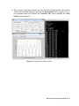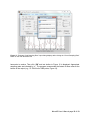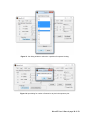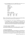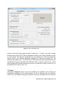
1
WaveAR User’s Manual
by
Blake J. Landry and Matthew J. Hancock
WaveAR User’s Manual page 1 of 19
WaveAR User’s Manual Contents
1. Introduction .............................................................................................................................................. 3
2. Installation ................................................................................................................................................ 3
2.1 Standalone executable........................................................................................................................ 3
2.2 MATLAB source code .......................................................................................................................... 4
3. Software use ............................................................................................................................................. 4
4. Description of the main WaveAR GUI ..................................................................................................... 10
4.1 Key parameters in the WaveAR GUI ................................................................................................. 11
4.2 Additional features of WaveAR......................................................................................................... 11
Sample rate estimation ....................................................................................................................... 11
Frequency spectrum ........................................................................................................................... 13
5. Data file format ....................................................................................................................................... 15
6. Example ................................................................................................................................................... 16
7. Companion program: VirtualWave ......................................................................................................... 17
7.1 Overview of VirtualWave GUI ........................................................................................................... 17
7.2 Output ............................................................................................................................................... 18
8. References .............................................................................................................................................. 19
WaveAR User’s Manual page 2 of 19
1. Introduction
This manual introduces the WaveAR software for parameter estimation from Stokes wave
measurements. An description of the algorithms in WaveAR may be found in (Landry et al.,
2012).
2. Installation
WaveAR may be run as a standalone executable or from MATLAB. This section outlines each
method. All files may be downloaded from http://vtchl.illinois.edu/software/, the WaveAR
webpage.
2.1 Standalone executable
WaveAR is run from a single executable file which requires the 20011b MATLAB Compiler
Runtime (MCR) available on the WaveAR webpage http://vtchl.illinois.edu/software/. The
following setup steps are recommended:
1) If you do not have MATLAB 2011b installed, you will need to install the free 2011b MCR.
(Note: the version number is important.)
2) Unzip the WaveAR folder which should unzip to a folder entitled WaveAR.
3) Within the WaveAR folder, find the correct executable file that corresponds to your
computer’s operating system (OS).
a. WaveAR_64.exe – executable for 64-bit Windows OS
b. WaveAR.exe – executable for Windows 32-bit OS
c. WaveAR.dmg – executable for Mac OS X
d. WaveAR– executable for Linux OS
4) To run the program, simply double click on the corresponding executable file (e.g. see
Figure 1 for example of 64-bit version exe).
Figure 1. WaveAR executable file for user specified OS (e.g., Windows 64-bit version shown).
WaveAR User’s Manual page 3 of 19
2.2 MATLAB source code
The WaveAR source code consists of two files: 1) WaveAR.fig contains the graphical user
interface (GUI) components and 2) WaveAR.m contains the main supporting functions. The
following setup steps are recommended:
1) Ensure MATLAB 2006 (or later) is installed with optimization toolbox.
2) Unzip the “WaveARsource” folder and navigate to this folder within the “Current
Directory” window in the MATLAB workspace.
3) Once in the folder, type WaveAR on the MATLAB command prompt and press the
“enter” key to run the program.
3. Software use
1) After installation, the following should appear for the corresponding installation method:
a. Standalone executable: When the executable starts, a black console window
appears (Figure 2, circle 1). Shortly after the console and main WaveAR
graphical user interface also appear (Figure 2, circle 2). Depending on computer
performance, the second window may load after a 30 second delay. For the
program to run, both windows must be open. If the console window is closed, the
main WaveAR interface will also close.
b. MATLAB source code: After typing WaveAR on the command prompt and
pressing the “enter” key, only the WaveAR GUI will appear (Figure 2, circle 2).
The black console window (Figure 2, circle 1) will not appear; the MATLAB
command window will display any printed output.
1
2
Figure 2. Black console window (red circle 1 and only for compiled versions) and main WaveAR GUI (red
circle 2) which appear shortly after running the WaveAR program.
WaveAR User’s Manual page 4 of 19
2) After the WaveAR window(s) appear, the user loads data by clicking the “Get Data”
button. This opens a standard file browser. The user simply selects the appropriate
comma separated value (.csv) file to process, and clicks the “Open” button to load and
process the file (Figure 3).
Figure 3. File browser dialog to select the .csv file for processing.
3) Once the data file is loaded successfully, the “WaveAR data fitting” window appears
(Figure 4) and the main WaveAR GUI now has “First Harmonic Parameters”, “Free
Second Harmonic Parameters”, and “Probe Data” button panels (Figure 5).
WaveAR User’s Manual page 5 of 19
Figure 4. WaveAR data fitting window appears after data is loaded.
Figure 5. Main WaveAR GUI with “First Harmonic Parameters”, “Free Second Harmonic Parameters”,
and “Probe Data” panels which appear after loading data.
WaveAR User’s Manual page 6 of 19
4) By adjusting the parameter sliders, the fitted and measured wave harmonic amplitudes
are matched across the entire domain (e.g., the wave tank). First and second harmonic
fits denoted by blue and red lines, resp. (Figure 6).
Figure 6. Data fitting by adjusting parameter sliders in the main WaveAR GUI. Blue and red lines denote
st
nd
the 1 and 2 harmonic amplitude fits, respectively.
WaveAR User’s Manual page 7 of 19
5) Once the fitted and measured profiles are close, the user can press the “AutoFit” button
to perform a least squares best fit (Figure 7). While “AutoFit” can be pressed at any time,
it is recommended to select initial parameters as a good first guess for the AutoFit
command.
Figure 7. Resulting parameter fit after pressing the AutoFit button. The blue and red lines virtually
coincide with the underlying data.
WaveAR User’s Manual page 8 of 19
6) After a proper fit has been achieved, the user can print the fitting results to the console
window (for immediate display) by pressing the “Print results” button (Figure 8) or to a
user specified data file by checking the “Create fit File” prior to pressing the “Print
results” button (Figure 9).
Figure 8. Results printed to console window.
WaveAR User’s Manual page 9 of 19
Figure 9. Results printed to output data file. Full path to output file is displayed.
4. Description of the main WaveAR GUI
In this section various elements on the WaveAR interface are discussed in greater detail.
1
2
5
6
7
3
8
4
9
10
11
12
Figure 10. The main WaveAR GUI.
WaveAR User’s Manual page 10 of 19
4.1 Key parameters in the WaveAR GUI
(1) Wave period: period of the water wave automatically loaded from data file (see data file
format section).
(2) Still water level: still water level (swl) of the experimental tank facility, automatically loaded
from data file (see data file format section).
(3) Lock checkboxes: locks the parameter so the value will remain unchanged during the
AutoFit data-fitting algorithm (listed in bullet 8).
(4) First harmonic fitting parameters:
A: incident wave amplitude
R: reflection coefficient
theta: phase of the reflection coefficient
L: attenuation coefficient
(5) file: displays the name of the loaded file.
(6) Longitudinal offset: offset for x-location values.
(7) errors: harmonic fit errors as presented in Eq. 8 of (Landry et al., 2012) .
(8) Free second harmonic fitting parameters:
A_2: incident wave amplitude
alpha_2: phase of the incident wave amplitude
R_2: reflection coefficient
theta_2: phase of the reflection coefficient
(9) Get Data button: allows the user to load data from a CSV file within a run folder.
(10) AutoFit button: automatically fits the slider parameters by least squares best fit to data.
(11) Print Results button (and Create Fit File checkbox): prints results to screen or to file (if
“Create Fit File” option checked).
(12) Probe Data button panel: allows further inspection of data.
View Spectrum: view spectrum at selected x-location.
Check Sampling Rate: determine sampling rate to avoid spectral leakage and aliasing.
4.2 Additional features of WaveAR
Sample rate estimation
WaveAR can help determine a sampling rate to avoid spectral leakage and aliasing. Load the
data as directed in the previous sections. The CSV data file does not require measurements for
all x-locations (measurements from single x-location is sufficient). After loading the data, press
the “Check Sampling Rate” button and the “Estimate Good Sampling Rate” window appears
(Figure 11). Enter the desired number of data samples (auto-filled with number of samples in
loaded data), the desired signal period, the maximum frequency to plot, and the number of
WaveAR User’s Manual page 11 of 19
Figure 11. “Estimate Good Sampling Rate” input dialog displays after clicking the “Check Sampling Rate”
button on the main WaveAR GUI.
harmonics to resolve. Then click “OK” and text similar to Figure 12 is displayed. Appropriate
sampling rates are indicated by “>”. The program recommends the fastest of these rates at the
bottom of the output (e.g., 97.3384 Hz for 2048 points, Figure 12).
WaveAR User’s Manual page 12 of 19
Figure 12. Output from the “Check Sampling Rate” button. Appropriate sampling rates are displayed with
a “>” next to the recommended rates.
Frequency spectrum
The spectrum at a given x-locations is produced by clicking the “View Spectrum” button in the
“Probe Data” panel on the main WaveAR GUI. A list dialog window appears for selecting the xlocation(s) to produce spectrums (Figure 13). Multiple selections are accomplished by holding
the shift key and/or ctrl key while clicking the desired positions. Click “OK” to confirm selection.
Another window appears prompting for “number of harmonics to plot up to” (Figure 14). After
specifying a value and clicking “OK”, a plot window entitled “Single-Sided Spectral Plots”
displays the spectra corresponding to the user-specified x-locations (Figure 15).
WaveAR User’s Manual page 13 of 19
Figure 13. List dialog window to select the x-positions for spectral viewing.
Figure 14. Input dialog for number of harmonics to plot in the spectrum plot.
WaveAR User’s Manual page 14 of 19
Figure 15. Example of spectrum plot for selected x-locations (i.e., 1.5, 2, 2.5, 3, 3.5, and 5 m).
5. Data file format
WaveAR loads data files in Comma Separated Value (CSV) format which can be created and
edited in text editors (e.g. WordPad, PsPad, TextEditor) or in Microsoft Excel. Figure 16 depicts
the CSV data file format corresponding to the fill color legend below.
Fill Color
Denotation
Tank parameters: cell A1: Wavemaker input frequency [Hz] (documentation only)
cell B1: Wavemaker input span [units] (documentation only)
cell C1: Tank still water depth [cm]
cell D1: Estimated wave period [sec]
cell E1: Measured water temperature [°C]
X-position [cm] of each column of surface wave measurements (row 2, column B
onward)
Sampling rate of the data [Hz] (cell A2)
Time values of the measured wave elevation [sec] (column A, row 3 downward)
Measured surface elevations for each x-position column [cm] (upper left cell B3)
WaveAR User’s Manual page 15 of 19
Figure 16. CSV data file displayed in MS Excel. Color corresponds to legend above.
6. Example
1) Open the WaveAR program.
2) Click “Get Data” button.
3) Browse the “example_data” folder within the “WaveAR” folder, select the
“autowavedata.csv” file, and click “Open” to load the file.
4) After the “WaveAR data fitting” window appears, manually adjust the sliders on the main
“WaveAR” program window. Helpful hint: start by adjusting the values A and R.
5) Once the fit is fairly close, press the “AutoFit” button to optimize the fit, least squares
error for each harmonic corresponding to the fit will update (see Figure 10, circle 7). The
theta sliders may need to be readjusted if they are positioned at 0 or 2π.
WaveAR User’s Manual page 16 of 19
6) Click the “Print Results” button (with the “Create Fit File” option unchecked), and the
following text should appear either in the console or command window:
T[sec] = 2.63
T_2[sec] = 1.315
h[cm] = 60
lambda[m] = 6.00794
lambda_2[m] = 2.45935
A[cm] = 5.00043
R = 0.999828
theta = 0.9999
A_2[cm] = 1
alpha_2 = 0
R_2 = 0
theta_2 = 0
L=0
X1[m] = 0
Xend[m] = 22
Error of fit for 1st harm = 0.0000
Error of fit for 2nd harm = 0.0001
X[m]
eta_rms [cm] eta_1 [cm]
0.0000
6.2543
8.7758
0.2500
6.9896
9.7168
0.5000
7.2150
9.9974
0.7500
6.8954
9.5984
.
.
.
eta_2 [cm]
1.1037
1.8147
2.0406
1.7212
.
Figure 17. Lambda and lambda_2 are the wavelengths of the first and free second harmonics,
respectively. The first harmonic, second harmonic, and rms amplitudes, denoted by eta_1, eta_2, and
eta_rms, are defined in Eqs. (6), (4) and (7) in (Landry et al., 2012), respectively.
7) Save the displayed results to a file by checking the “Create Fit File” box and pressing
the “Print Results” button. The resulting data files “autowavedata.fit” and
“autowavedata.fig” (a text fitting file and MATLAB figure file, respectively) will be saved
to the same “run” folder where the data was initially loaded. If a fitting parameter was
locked (by using the checkboxes) the resulting data file names will be appended to
indicate what was locked (e.g. “autowavedata_hold_R.fit” indicates that R was locked).
7. Companion program: VirtualWave
Similar to WaveAR, VirtualWave may be run as a standalone executable or in MATLAB. The
user should select the appropriate file (same convention as WaveAR) to run the software.
7.1 Overview of VirtualWave GUI
The VirtualWave GUI has panel groups for each parameter set, e.g., first harmonic wave,
physical tank, data sampling free second harmonic, and visualization parameters (Figure 18).
The first and free second harmonic parameters for the VirtualWave program are the same as
those presented in the main text for the WaveAR software. Additional data sampling parameters
may be defined, such as the sampling rate fs and the number of samples n for each of the
WaveAR User’s Manual page 17 of 19
Figure 17. Main VirtualWave GUI.
selected virtual wave gage (probe) locations. Pressing the “?” button in the data sampling
parameter panel executes the “Estimate appropriate sampling rate” feature described on page
11 of this manual. This estimate is explained in Eq. (9) in (Landry et al., 2012). By entering the
desired values in the “Estimate appropriate sampling rate” window and pressing “Ok”, the
estimated rate replaces the “?” text in the button. Clicking the button again copies that value into
the Sampling frequency value field. Data fields that require an array of numbers (e.g., Virtual
probe locations) follow the MATLAB array convention. For example, to create a vector from 0 to
22 spaced by 0.25, enter [0: 0.25 : 22].
7.2 Output
Pressing the “Generate” button in the main VirtualWave GUI generates a plot window with
instantaneous snapshots of the surface elevation as well as harmonic and rms amplitudes
(Figure 19). If the “Enable file saving” was checked on the main VirtualWave GUI, the user may
WaveAR User’s Manual page 18 of 19
Figure 18. VirtualWave results window. Top: instantaneous surface elevation plotted at different times.
Middle: first and second harmonic amplitudes. Both continuous and sampled (at fixed probe locations)
versions are shown. Bottom: rms amplitude. Both continuous and sampled versions are shown.
then save the output to file. The output file may then be loaded into WaveAR by following the
instructions in the “Software use” section above.
8. References
Landry, B.J., Hancock, M.J., Mei, C.C., García, M.H., 2012. WaveAR: A software tool for calculating
parameters for water waves with incident and reflected components. Computers & Geoscience
submitted.
WaveAR User’s Manual page 19 of 19