Download Manual - Department of Computing

Inductive Learning of Answer Set Programs
v2.4.2
User Manual
Authors:
Mark Law &
Alessandra Russo &
Krysia Broda
July 3, 2015
Inductive Learning of Answer Set Programs - User Manual
M. Law, A. Russo, K. Broda
Contents
1 Background and Installation
2
1.1
Answer Set Programming . . . . . . . . . . . . . . . . . . . . . . . . . . . . . . . . . . . . . . . . . . .
2
1.2
Installation . . . . . . . . . . . . . . . . . . . . . . . . . . . . . . . . . . . . . . . . . . . . . . . . . . .
4
1.2.1
Linux . . . . . . . . . . . . . . . . . . . . . . . . . . . . . . . . . . . . . . . . . . . . . . . . . .
4
1.2.2
Mac OSX . . . . . . . . . . . . . . . . . . . . . . . . . . . . . . . . . . . . . . . . . . . . . . . .
4
How to run ILASP . . . . . . . . . . . . . . . . . . . . . . . . . . . . . . . . . . . . . . . . . . . . . . .
5
1.3.1
5
1.3
Options . . . . . . . . . . . . . . . . . . . . . . . . . . . . . . . . . . . . . . . . . . . . . . . . .
2 Learning from Answer Sets
6
2.1
Specifying simple learning tasks in ILASP . . . . . . . . . . . . . . . . . . . . . . . . . . . . . . . . . .
6
2.2
Language Bias . . . . . . . . . . . . . . . . . . . . . . . . . . . . . . . . . . . . . . . . . . . . . . . . .
7
2.2.1
Extra options for mode declarations . . . . . . . . . . . . . . . . . . . . . . . . . . . . . . . . .
8
Example Tasks . . . . . . . . . . . . . . . . . . . . . . . . . . . . . . . . . . . . . . . . . . . . . . . . .
8
2.3.1
9
2.3
Sudoku . . . . . . . . . . . . . . . . . . . . . . . . . . . . . . . . . . . . . . . . . . . . . . . . .
3 Learning Weak Constraints using ILASP
11
3.1
Language Bias for Weak Constraints . . . . . . . . . . . . . . . . . . . . . . . . . . . . . . . . . . . . . 12
3.2
Example Tasks . . . . . . . . . . . . . . . . . . . . . . . . . . . . . . . . . . . . . . . . . . . . . . . . . 14
3.2.1
Scheduling
. . . . . . . . . . . . . . . . . . . . . . . . . . . . . . . . . . . . . . . . . . . . . . . 14
4 Specifying Learning Tasks with Noise in ILASP
4.1
17
Example: Noisy Sudoku . . . . . . . . . . . . . . . . . . . . . . . . . . . . . . . . . . . . . . . . . . . . 17
5 Hypothesis length
19
i
Inductive Learning of Answer Set Programs - User Manual
M. Law, A. Russo, K. Broda
Abstract
ILASP[1] (Inductive Learning of Answer Set Programs) is a system for learning ASP (Answer Set Programming) programs from examples. It is capable of learning normal rules, choice rules and constraints through positive
and negative examples of partial answer sets. ILASP can also learn preferences, represented as weak constraints
in ASP by considering example ordered pairs of partial answer sets.
1
Inductive Learning of Answer Set Programs - User Manual
1
M. Law, A. Russo, K. Broda
Background and Installation
Inductive Logic Programming (ILP)[2] is the field of research considering logic-based machine learning. The goal
is to find an hypothesis which, together with some given background knowledge, entails a set of positive examples
and does not entail any of a set of negative examples. Mostly, ILP research has addressed the problem of learning
definite clauses intended for use in Prolog programs.
More recently, there has been work on learning under the stable model semantics[3]. In [4], the concepts of brave
and cautious induction were introduced. The task of brave induction is to find an hypothesis H such that B ∪ H
(the background knowledge augmented with H) has at least one answer set which satisfies the examples; cautious
induction on the other hand requires that B ∪ H is has at least one answer set and that every answer set satisfies
the examples.
Early algorithms such as [5, 6] solved brave induction tasks. In [7], we gave examples of hypotheses which could not
be learned by brave or cautious induction alone and presented a new learning framework Learning from Answer Sets
which is capable of expressing both brave and cautious induction in the same learning task.
Our algorithm, ILASP (Inductive Learning of Answer Set Programs) is sound and complete with respect to the
optimal (shortest) Learning from Answer Sets tasks. In [8], we presented an extension to our Learning from Answer
Sets framework, Learning from Ordered Answer Sets which is capable of learning preferences represented as weak
constraints.
ILASP2, is sound and complete with respect to the optimal solutions of any Learning from Ordered Answer Sets
task.
1.1
Answer Set Programming
This document should not be used as an introduction to Answer Set Programming (ASP). Good introductions to
ASP are [9, 10, 11]. In this section, we introduce the subset of ASP which ILASP uses.
In this document, we consider a literal to be either an atom, the negation as failure of an atom (written not a for
an atom a) or a comparison between two terms such as X > 2 or 4! = Y.
A normal rule is written: h :- b1 , . . . , bn where h1 is an atom and b1 . . . bn are literals. Such a normal rule is read as
“if b1 . . . bn are all true, then h must also be true”.
A normal logic program is a set of normal rules. The Herbrand Base of a program P (written HBP ) is the set of all
ground atoms which can be constructed using predicate names, constant symbols and function symbols in P . The
Herbrand Interpretations of P are the subsets of HBP and each interpretation I is interpreted as assigning any atom
in I to be true and any other atom to false.
To solve a normal program P for answer sets, it is first replaced with an equivalent ground program. An interpretation
I is an answer set of a ground program P if and only if it is a minimal model of the reduct of P with respect to I.
This reduct (written P I ) is construced in two steps: firstly, remove any rule in P which contains the negation of an
atom in I; secondly, remove any remaining negative literals from the remaining rules. For more details, see any of
the references mentioned at the beginning of this section.
A (hard) constraint, is essentially a normal rule without a head. This empty head is often read as false. The meaning
of a constraint :- b1 , . . . , bn is that if b1 . . . bn are satisfied by an interpretation, then it cannot be an answer set.
A choice rule is written l{h1 ; . . . ; hm }u :- b1 , . . . , bn . where l and u are integers such that 0 ≤ l ≤ u ≤ n. Informally,
the meaning of such a rule is that if the body is satisfied then between l and u of the atoms h1 , . . . , hn must be
satisfied. A simplified version of the reduct for programs containing normal rules, choice rules and constraints can
be found at [12].
The final type of rule that we allow in ILASP is called a weak constraint. Weak constraints do not effect the answer
sets of a program P , but they specify an ordering over the answer sets of P saying which answer sets are preferred
to others. ASP can solve programs for optimal answer sets (answer sets which are not less preferred than any other
answer set).
2
Inductive Learning of Answer Set Programs - User Manual
M. Law, A. Russo, K. Broda
Example 1.1. Consider the program:
coin(1..3). % Note that this is a shorthand for coin(1). coin(2). coin(3).
1 { heads(C); tails(C) } 1 :- coin(C).
:~ heads(C).[1@2, C]
:~ tails(C).[1@1, C]
The choice rule in this program says that every coin is either heads or tails. This naturally leads to 8 answer sets in
which the 3 coins take every combination of values.
The first weak constraint has priority 2 (read from the “@2”), whereas the second has priority 1. This means that the
first weak constraint is more important and we solve this first. By this, we mean we select the answer sets which are
best according to this weak constraint. If there is more than one such answer set, then we compare these remaining
answer sets using the lower priority weak constraint.
The first weak constraint says that we must pay a penaulty of 1 for every coin that takes the value heads. This
means that if we have 0 coins which are heads we pay 0, if we have 1 head we pay 1 etc. This means that the only
optimal answer set is the one in which all coins are tails.
The list terms appearing at the end of a weak constraint (after the priority level) are there to specify which constraints
should be considered unique; for example, if we ground the first weak constraint in the previous program we get:
coin(1..3). % Note that this is a shorthand for coin(1). coin(2). coin(3).
:~ heads(1).[1@2, 1]
:~ heads(2).[1@2, 2]
:~ heads(3).[1@2, 3]
This means that each weak constraint is considered unique, and so we must pay the penaulty for each weak constraint
whose body is satisfied.
Consider instead the similar program:
coin(1..3). % Note that this is a shorthand for coin(1). coin(2). coin(3).
1 { heads(C); tails(C) } 1 :- coin(C).
:~ heads(C).[1@2]
:~ tails(C).[1@1, C]
The answer sets of this program remain the same, but now when we ground the first weak constraint we get:
coin(1..3). % Note that this is a shorthand for coin(1). coin(2). coin(3).
:~ heads(1).[1@2]
:~ heads(2).[1@2]
:~ heads(3).[1@2]
As “[1@2]” occurs for all three weak constraints, we only have to pay the penaulty once if we have any heads. This
means that we pay penaulty 0 if we have no heads, and penaulty 1 if we have 1, 2 or 3 heads.
More formally, a weak constraint is written :∼ b1 , . . . , bn .[w@l, t1 , . . . , tm ] where b1 , . . . , bn are literals, w is either a
variable or an integer called the weight, l is an integer called the level and t1 , . . . , tm are terms. A ground weak
constraint of this form has the meaning that if b1 , . . . , bn are satisfied by an answer set A then we must pay the
penaulty w. The terms ti are to specify which of the ground weak constraints should be considered distinct (if
two weak constraints have the same w, l and t1 , . . . , tn we will only pay the penaulty once, even if both bodies are
satisfied). The aim is to find an answer set which pays the minimum penaulty. The idea of the levels are that
we should solve the higher levels first (considering them as a higher priority). Only if two answer sets pay equal
penaulties for all levels above l do we consider the weak constraints of level l.
3
Inductive Learning of Answer Set Programs - User Manual
1.2
M. Law, A. Russo, K. Broda
Installation
1.2.1
Linux
Note that although in theory ILASP should work on any Linux distribution, we have only tested it on Ubuntu 14.04.
Clingo. [13] ILASP depends on clingo version 4.3.0. It is important that exactly this version1 is used due to differences in clingo’s built in scripting language in later versions. At the time of writing clingo 4.3.0 can be downloaded
from http://downloads.sourceforge.net/project/potassco/clingo/4.3.0/clingo-4.3.0-x86_64-linux.tar.
gz. The clingo executable should then be copied somewhere in your PATH. Our recommended approach is to copy
the executable into the /usr/local/bin/ directory.
Poco. ILASP uses the poco library. This library can be installed in Ubuntu using the command sudo apt-get
install libpoco-dev.
The current version of ILASP for linux can be obtained from http://sourceforge.net/projects/spikeimperial/
files/ILASP/. It is recommended that you again copy the executable to /usr/local/bin/.
1.2.2
Mac OSX
ILASP has been built and tested on OSX 10.10 (Yosemite).
Clingo. [13] ILASP depends on clingo version 4.3.0. It is important that exactly this version1 is used due to
differences in clingo’s built in scripting language in later versions. At the time of writing clingo 4.3.0 can be downloaded from http://downloads.sourceforge.net/project/potassco/clingo/4.3.0/clingo-4.3.0-macos-10.
9.tar.gz. The clingo executable should then be copied somewhere in your PATH. Our recommended approach is to
copy the executable into the /usr/local/bin/ directory.
Poco. ILASP uses the poco library. This library can either be downloaded from http://pocoproject.org/
download/ or installed in OSX using the brew2 package manager (brew install poco).
The current version of ILASP for OSX can be obtained from http://sourceforge.net/projects/spikeimperial/
files/ILASP/. It is recommended that you again copy the executable to /usr/local/bin/.
1 Note
2 for
that if you decide to compile clingo 4.3.0 from source, it is vital that you compile it with Lua support
details of how to install brew see http://brew.sh.
4
Inductive Learning of Answer Set Programs - User Manual
1.3
M. Law, A. Russo, K. Broda
How to run ILASP
Once you have installed ILASP, you should be able to run the example tasks available at http://sourceforge.net/
projects/spikeimperial/files/ILASP/. Assuming you have an ILASP task stored at the location “path to task”,
you can use ILASP to solve this task for an optimal solution using the following command:
ILASP path_to_task
1.3.1
Options
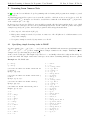
ILASP has several options which can be given before or after the path to the task which is to be solved. These are
summarised by table 1
Option
-s
-t
-q
Example usage
ILASP -s path to task
ILASP -t path to task
ILASP -q path to task
Description
Print the search space for the task at path to task.
Print the ILASP ASP encoding for the task at path to task and exit.
Solve the task at path to task as normal, but only print the hypothesis.
Table 1: A summary of the main options which can be passed to ILASP.
5
Inductive Learning of Answer Set Programs - User Manual
2
M. Law, A. Russo, K. Broda
Learning from Answer Sets
In [7] we specified a new Inductive Logic Programming task for learning ASP programs from examples of partial
interpretations.
A partial interpretation E is a pair of sets of atoms E inc and E exc , called the inclusions and exclusions of E. We
write E as hE inc , E exc i. An answer set A is said to extend E if it contains all of the inclusions (E inc ⊆ A) and none
of the exclusions (E exc ∩ A = ∅)).
In Learning from Answer Sets (ILPLAS ), given an ASP program B called the background knowledge, a set of ASP
rules S called the search space and two sets of partial interpretations E + and E − called the positive and negative
examples respectively, the goal is to find another program H called an hypothesis such that:
1. H is composed of the rules in S (H ⊆ S).
2. Each positive example is extended by at least one answer set of B ∪ H (this can be a different answer set for
each positive example).
3. No negative example is extended by any answer set of B ∪ H.
2.1
Specifying simple learning tasks in ILASP
exc
exc
inc
A positive example h{einc
1 , . . . em }, {e1 , . . . , en }i can be specified in ILASP as the statement: #pos(example name,
exc
exc
inc
inc
{e1 , . . . , em }, {e1 , . . . , en }). where example name is a unique identifier for the example. Similarly a negative
example can be specified using the predicate #neg.
A rule r in the search space with length l is specified as l ∼ r and finally, rules in the background knowledge are
specified as normal. The length of rules in the search space is used when determining which hypotheses are optimal.
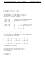
Example 2.1. The ILASP task:
p :- not q.
q :- not p.
1
1
3
3
3
3
2
2
2
2
3
3
3
3
2
2
2
2
2
2
2
2
3
3
3
3
3
3
3
3
% At least one answer set should contain but not
% contain r.
#pos(p1, {q}, {r}).
% At least one answer set should contain both q
% and r.
#pos(p2, {q, r}, {}).
% At least one answer set should contain p.
#pos(p3, {p}, {}).
% No answer set should contain both p and r.
#neg(n1, {p, r}, {}).
1
1
2
2
2
2
1
1
2
2
1
1
2
2
~
~
~
~
~
~
~
~
~
~
~
~
~
~
r.
s.
r :- not p.
r :- p.
s :- not p.
s :- p.
:- not p.
:- p.
s :- not r.
s :- r.
:- not r.
:- r.
r :- not s.
r :- s.
6
~
~
~
~
~
~
~
~
~
~
~
~
~
~
~
~
~
~
~
~
~
~
~
~
~
~
~
~
~
~
:- not s.
:- s.
s :- not p, not r.
s :- p, not r.
s :- not p, r.
s :- p, r.
:- not p, not r.
:- p, not r.
:- not p, r.
:- p, r.
r :- not p, not s.
r :- p, not s.
r :- not p, s.
r :- p, s.
:- not p, not s.
:- p, not s.
:- not p, s.
:- p, s.
:- not r, not s.
:- r, not s.
:- not r, s.
:- r, s.
:- not p, not r, not s.
:- p, not r, not s.
:- not p, r, not s.
:- p, r, not s.
:- not p, not r, s.
:- p, not r, s.
:- not p, r, s.
:- p, r, s.
Inductive Learning of Answer Set Programs - User Manual
M. Law, A. Russo, K. Broda
when solved with ILASP gives the output:
r :- not p, not s.
s :- not r.
Pre-processing
Solve time
Total
: 0.003s
: 0.018s
: 0.021s
In this case, the answer sets of B ∪ H are {p, s}, {q, s} and {q, r}. Note that these three answer sets extend the
three positive examples, and no answer set extends the negative example.
2.2
Language Bias
The ILASP procedure depends on a search space of possible hypotheses in which it should search for inductive
solutions. Although in ILASP the search space can be given in full as in the previous section, the conventional way
of specifying this search space is to give a language bias specified by mode declarations (this is sometimes called a
mode bias).
A placeholder is a term var(t) or const(t) for some constant term t. The idea is that these can be replaced by
any variable or constant (respectively) of type t.
Each constant c which is allowed to replace a const term of type t should be specified as #constant(t, c)
A mode declaration is a ground atom whose arguments can be placeholders. An atom a is compatible with a mode
declaration m if each of the placeholder constants and placeholder variables in m has been replaced by a constant or
variable of the correct type (the user does not have to list the variables which can be used, but ILASP will ensure
that no variable occurs twice in the same rule with a different type).
There are three types of mode declaration: modeh the normal head declarations; modeha, the aggregate head
declarations; modeb, the body declarations; and modeo, the optimisation body declarations. Each mode declaration
can also be specified with a recall, which is an integer specifying the maximum number of times that mode declaration
can be used in each rule.
A user can specify a mode declaration stating that the predicate p with arity 1 can be used in each rule up to two
times with a single variable of type type1, for example, as #modeb(2, p(var(type1))).
The maximum number of variables in any rule can be specified using the predicate #maxv; for example #maxv(2)
states that at most 2 variables can be used in each rule of the hypothesis. Similarly, #max penaulty specifies an
upper bound on the size of the hypothesis returned. By default, this is 15. Lower values for this are likely to increase
the speed of computation, but in some cases larger bounds are needed (as in the sudoku example in the next section).
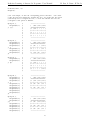
Example 2.2. The language bias:
#modeha(r(var(t1), const(t2)))
#modeh(p)
#modeb(1, p)
#modeb(2, q(var(t1)))
#constant(t2, c1)
#constant(t2, c2)
#maxv(2).
Leads to the search space:
:::::-
q(V1).
p.
not p.
q(V1), p.
q(V1), not p.
p.
p :- q(V1).
0 { r(V1, c1) } 1 :- q(V1).
7
Inductive Learning of Answer Set Programs - User Manual
0 { r(V1, c1) } 1 :- q(V1), p.
0 { r(V1, c1) } 1 :- q(V1), not p.
0
0
0
0
0
0
{
{
{
{
{
{
r(V1,
r(V1,
r(V1,
r(V1,
r(V1,
r(V1,
c2)
c2)
c2)
c2)
c2)
c2)
}
}
}
}
}
}
1
1
1
1
1
1
::::::-
q(V1).
q(V1),
q(V1),
q(V1),
q(V1),
q(V1),
0
0
0
1
1
1
1
1
1
{
{
{
{
{
{
{
{
{
r(V1,
r(V1,
r(V1,
r(V1,
r(V1,
r(V1,
r(V1,
r(V1,
r(V1,
c1);
c1);
c1);
c1);
c1);
c1);
c1);
c1);
c1);
r(V1,
r(V1,
r(V1,
r(V1,
r(V1,
r(V1,
r(V1,
r(V1,
r(V1,
c2)
c2)
c2)
c2)
c2)
c2)
c2)
c2)
c2)
}
}
}
}
}
}
}
}
}
1
1
1
1
1
1
2
2
2
:::::::::-
q(V1).
q(V1),
q(V1),
q(V1).
q(V1),
q(V1),
q(V1).
q(V1),
q(V1),
0
0
0
1
1
{
{
{
{
{
r(V1,
r(V1,
r(V1,
r(V1,
r(V1,
c1);
c1);
c1);
c1);
c1);
r(V2,
r(V2,
r(V2,
r(V2,
r(V2,
c1)
c1)
c1)
c1)
c1)
}
}
}
}
}
1
1
1
1
1
:::::-
q(V1),
q(V1),
q(V1),
q(V1),
q(V1),
q(V2).
q(V2), p.
p.
q(V2), not p.
not p.
p.
not p.
p.
not p.
p.
not p.
q(V2).
q(V2), p.
q(V2), not p.
q(V2).
q(V2), p.
M. Law, A. Russo, K. Broda
1
1
1
1
{
{
{
{
r(V1,
r(V1,
r(V1,
r(V1,
c1);
c1);
c1);
c1);
r(V2,
r(V2,
r(V2,
r(V2,
c1)
c1)
c1)
c1)
}
}
}
}
1
2
2
2
::::-
q(V1),
q(V1),
q(V1),
q(V1),
q(V2), not p.
q(V2).
q(V2), p.
q(V2), not p.
0
0
0
1
1
1
1
1
1
{
{
{
{
{
{
{
{
{
r(V1,
r(V1,
r(V1,
r(V1,
r(V1,
r(V1,
r(V1,
r(V1,
r(V1,
c1);
c1);
c1);
c1);
c1);
c1);
c1);
c1);
c1);
r(V2,
r(V2,
r(V2,
r(V2,
r(V2,
r(V2,
r(V2,
r(V2,
r(V2,
c2)
c2)
c2)
c2)
c2)
c2)
c2)
c2)
c2)
}
}
}
}
}
}
}
}
}
1
1
1
1
1
1
2
2
2
:::::::::-
q(V1),
q(V1),
q(V1),
q(V1),
q(V1),
q(V1),
q(V1),
q(V1),
q(V1),
q(V2).
q(V2),
q(V2),
q(V2).
q(V2),
q(V2),
q(V2).
q(V2),
q(V2),
0
0
0
1
1
1
1
1
1
{
{
{
{
{
{
{
{
{
r(V1,
r(V1,
r(V1,
r(V1,
r(V1,
r(V1,
r(V1,
r(V1,
r(V1,
c2);
c2);
c2);
c2);
c2);
c2);
c2);
c2);
c2);
r(V2,
r(V2,
r(V2,
r(V2,
r(V2,
r(V2,
r(V2,
r(V2,
r(V2,
c2)
c2)
c2)
c2)
c2)
c2)
c2)
c2)
c2)
}
}
}
}
}
}
}
}
}
1
1
1
1
1
1
2
2
2
:::::::::-
q(V1),
q(V1),
q(V1),
q(V1),
q(V1),
q(V1),
q(V1),
q(V1),
q(V1),
q(V2).
q(V2),
q(V2),
q(V2).
q(V2),
q(V2),
q(V2).
q(V2),
q(V2),
p.
not p.
p.
not p.
p.
not p.
p.
not p.
p.
not p.
p.
not p.
Note that ILASP will try to omit rules which will never appear in an optimal inductive solution; for example, as p
:- q(V1), q(V2). is satisfied if and only if p :- q(V1). is satisfied, the former will never be part of an optimal
solution, and so is not generated.
For details of how we assign lengths to rules in the search space, see section 5.
2.2.1
Extra options for mode declarations
A final argument may be given to any mode declarations, which is a tuple to restrict the use of this mode declaration.
The idea is that this can be used to further steer the search away from hypotheses which are uninteresting and thus
improve the speed of the search.
This final argument is a tuple which may contain the any of the constants: anti reflexive, symmetric, positive.
The meaning of these constants is as follows:
1. anti reflexive is intended for use on predicates of arity 2. It means that the predicate should not be generated
with 1 variable repeated for both arguments; for example, p(X,X) is not compatible with
#modeh(p(var(t),var(t)),(anti reflexive)).
2. symmetric is intended for use on predicates of arity 2. It means that, for example, given the mode declaration
#modeh(p(var(t),var(t)),(symmetric)), rules containing p(X, Y) are considered equivalent to the same
rule replaced with p(Y, X) and, as such, only one is generated.
3. positive means that the negation as failure of the predicate in the mode declaration should not be generated.
Other options, aimed mainly at choice rules (as it is very easy to generate a search space with a massive number
of choice rules) are #disallow multiple head variables, which prevents more than one variable being used in the
head of a rule; #minh and #maxh which are predicates of arity 1 specifying the minimum and maximum number of
literals which can occur in the head of a choice rule.
2.3
Example Tasks
In this section, we give example learning tasks encoded in ILASP. The first shows how ILASP can be used to learn
the rules of sudoku. Further examples may follow in later editions of this manual.
8
Inductive Learning of Answer Set Programs - User Manual
2.3.1
M. Law, A. Russo, K. Broda
Sudoku
Consider the following learning task whose background knowledge contains the definitions of what it means to be a
cell, and for two cells to be in the same row, column and block:
cell((1..4,1..4)).
block((X,
block((X,
block((X,
block((X,
Y),
Y),
Y),
Y),
tl)
tr)
bl)
br)
::::-
cell((X,
cell((X,
cell((X,
cell((X,
Y)),
Y)),
Y)),
Y)),
X
X
X
X
<
>
<
>
3,
2,
3,
2,
Y
Y
Y
Y
<
<
>
>
3.
3.
2.
2.
same_row((X1,Y),(X2,Y)) :- X1 != X2, cell((X1,Y)), cell((X2, Y)).
same_col((X,Y1),(X,Y2)) :- Y1 != Y2, cell((X,Y1)), cell((X, Y2)).
same_block(C1,C2) :- block(C1, B), block(C2, B), C1 != C2.
#pos(a, {
value((1,
value((1,
value((1,
value((1,
value((2,
}, {
value((1,
value((1,
value((1,
}).
1),
2),
3),
4),
3),
1),
2),
3),
4),
2)
1), 2),
1), 3),
1), 4)
% This positive examples says that there should be at
% least one answer set of B union H which represents a
% board extending the partial board:
%
%
#-------#-------#
%
| 1 : 2 | 3 : 4 |
%
| - + - | - + - | such that the first cell
%
|
:
| 2 :
| does not also contain a
%
#-------#-------# value other than 1.
%
|
:
|
:
|
%
| - + - | - + - |
%
|
:
|
:
|
%
#-------#-------#
#neg(b, { value((1, 1), 1), value((1, 3), 1) },{}).
#neg(c, { value((1, 1), 1), value((3, 1), 1) },{}).
#neg(d, { value((1, 1), 1), value((2, 2), 1) },{}).
% The negative examples say that there should be no answer set corresponding to a
% board extending any of the partial boards:
%
%
#-------#-------#
#-------#-------#
#-------#-------#
%
| 1 :
| 1 :
|
| 1 :
|
:
|
| 1 :
|
:
|
%
| - + - | - + - |
| - + - | - + - |
| - + - | - + - |
%
|
:
|
:
|
|
:
|
:
|
|
: 1 |
:
|
%
#-------#-------#
#-------#-------#
#-------#-------#
%
|
:
|
:
|
| 1 :
|
:
|
|
:
|
:
|
%
| - + - | - + - |
| - + - | - + - |
| - + - | - + - |
%
|
:
|
:
|
|
:
|
:
|
|
:
|
:
|
%
#-------#-------#
#-------#-------#
#-------#-------#
#modeha(value(var(cell),const(number))).
#modeb(2,value(var(cell),var(val))).
#modeb(1,same_row(var(cell), var(cell)), (anti_reflexive)).
#modeb(1,same_block(var(cell), var(cell)), (anti_reflexive)).
#modeb(1,same_col(var(cell), var(cell)), (anti_reflexive)).
#modeb(1,cell(var(cell))).
#constant(number,
#constant(number,
#constant(number,
#constant(number,
1).
2).
3).
4).
9
Inductive Learning of Answer Set Programs - User Manual
M. Law, A. Russo, K. Broda
#minhl(4).
#maxhl(4).
#disallow_multiple_head_variables.
#max_penaulty(30).
Calling ILASP on this task will give an output similar to:
:- value(V0,V1), value(V2,V1), same_col(V0, V2).
:- value(V0,V1), value(V2,V1), same_block(V0, V2).
:- value(V0,V1), value(V2,V1), same_row(V2, V0).
1 {value(V0,4); value(V0,3); value(V0,2); value(V0,1) } 1 :- cell(V0).
Pre-processing
Solve time
Total
: 0.028s
: 0.91s
: 0.938s
This hypothesis represents the rules of a 4 × 4 version of the popular game of sudoku. The choice rule says that every
cell takes exactly one value between 1 and 4 and the three constraints rule out the 3 cases of illegal board where
values occur more than once in the same column, block or row.
10
Inductive Learning of Answer Set Programs - User Manual
3
M. Law, A. Russo, K. Broda
Learning Weak Constraints using ILASP
In [8], we defined a new task, Learning from Ordered Answer Sets which extends Learning from Answer Sets with
the capability of learning weak constraints. As positive and negative examples do not incentivise learning weak
constraints, we introduced a new notion of ordering examples. These come in two kinds, brave and cautious.
Definition 3.1. An ordering example is a tuple o = he1 , e2i where e1 and e2 are partial interpretations. An ASP
program P bravely respects o if and only if ∃A1 , A2 ∈ AS(P ) such that A1 extends e1 , A2 extends e2 and A1 P A2 .
P cautiously respects o if and only if for each A1 , A2 ∈ AS(P ) such that A1 extends e1 and A2 extends e2 , it is the
case that A1 P A2 .
The partial interpretations in ordering examples must be positive examples. Given two positive examples e1 and e2
with identifiers id 1 and id 2, the ordering example he1 , e2 i can be expressed as #brave ordering(order name, id1 , id2 )
or #cautious ordering(order name, id1 , id2 ) where order name is an optional identifier for the ordering example.
Example 3.2. Consider a learning task with positive examples #pos(p1, {p}, {}) and #pos(p2, {}, {p}) and a single
ordering example #brave ordering(o1, p1, p2). ILASP will search for the shortest hypothesis H such that B ∪ H
has answer sets to cover each positive example, and there is at least one answer set which contains p which is more
optimal than at least one answer set which does not contain p.
If we consider the same positive examples, but now with the ordering example #pos(p2, {}, {p}), then ILASP will
search for an hypothesis H such that B ∪ H has answer sets to cover each positive example, and every answer set
which contains p is more optimal than every answer set which does not contain p.
We now define the notion of Learning from Ordered Answer Sets by extending Learning from Answer Sets with
ordering examples.
Definition 3.3. A Learning from Ordered Answer Sets task is a tuple T = hB, SM , E + , E − , Ob , Oc i where B is as
ASP program, called the background knowledge, SM is the search space defined by a mode bias with ordering M ,
E + and E − are sets of partial interpretations called, respectively, positive and negative examples, and Ob and Oc are
both sets of ordering examples over E + . An hypothesis H is an inductive solution of T (written H ∈ ILPLOAS (T ))
if and only if:
LAS
, E + , E − i)3
1. H 0 ∈ ILPLAS (hB, SM
2. ∀o ∈ Ob B ∪ H bravely respects o
3. ∀o ∈ Oc B ∪ H cautiously respects o
Example 3.4. Consider the learning task:
animal(cat).
animal(dog).
0 { own(A) } 1 :- animal(A).
animal(fish).
eats(cat, fish).
#pos(p1, { own(fish) }, { own(cat) }).
#pos(p3, { own(dog), own(cat), own(fish) }, {}).
#pos(best, { own(dog), own(fish) }, { own(cat) }).
#brave_ordering(best, p1).
#brave_ordering(best, p2).
#brave_ordering(best, p3).
#cautious_ordering(best, p4).
3 S LAS
M
eats(dog, cat).
#pos(p2, { own(cat) }, { own(dog), own(fish)}).
#pos(p4, { own(dog)}, { own(fish) }).
%
%
%
%
%
%
%
%
%
%
%
is the subset of SM which are not weak constraints.
11
These ordering examples all use an example "best" in
which a dog and a fish is owned and a cat is not owned.
"best" is better than some situations
own a fish but no cat.
"best" is better than some situations
own a cat but no fish or dog.
"best" is better than some situations
own a fish, dog and cat.
"best" is better than every situation
we own a dog but no fish.
where we
where we
where we
in which
Inductive Learning of Answer Set Programs - User Manual
1
1
1
1
1
1
1
1
2
2
2
2
2
2
2
2
2
2
2
2
2
2
2
2
2
2
2
2
3
~
~
~
~
~
~
~
~
~
~
~
~
~
~
~
~
~
~
~
~
~
~
~
~
~
~
~
~
~
M. Law, A. Russo, K. Broda
3 ~ :~ eats(V0, V1), not own(V0),
not own(V1).[-1@2, 32, V0, V1]
3 ~ :~ eats(V0, V1), own(V0),
not own(V1).[1@1, 33, V0, V1]
3 ~ :~ eats(V0, V1), own(V0),
not own(V1).[1@2, 34, V0, V1]
3 ~ :~ eats(V0, V1), own(V0),
not own(V1).[-1@1, 35, V0, V1]
3 ~ :~ eats(V0, V1), own(V0),
not own(V1).[-1@2, 36, V0, V1]
3 ~ :~ not eats(V0, V1), own(V0),
own(V1).[1@1, 37, V0, V1]
3 ~ :~ not eats(V0, V1), own(V0),
own(V1).[1@2, 38, V0, V1]
3 ~ :~ not eats(V0, V1), own(V0),
own(V1).[-1@1, 39, V0, V1]
3 ~ :~ not eats(V0, V1), own(V0),
own(V1).[-1@2, 40, V0, V1]
3 ~ :~ not eats(V1, V0), own(V0),
own(V1).[1@1, 41, V0, V1]
3 ~ :~ not eats(V1, V0), own(V0),
own(V1).[1@2, 42, V0, V1]
3 ~ :~ not eats(V1, V0), own(V0),
own(V1).[-1@1, 43, V0, V1]
3 ~ :~ not eats(V1, V0), own(V0),
own(V1).[-1@2, 44, V0, V1]
3 ~ :~ eats(V0, V1), own(V0),
own(V1).[1@1, 45, V0, V1]
3 ~ :~ eats(V0, V1), own(V0),
own(V1).[1@2, 46, V0, V1]
3 ~ :~ eats(V0, V1), own(V0),
own(V1).[-1@1, 47, V0, V1]
3 ~ :~ eats(V0, V1), own(V0),
own(V1).[-1@2, 48, V0, V1]
:~
:~
:~
:~
:~
:~
:~
:~
:~
:~
:~
:~
:~
:~
:~
:~
:~
:~
:~
:~
:~
:~
:~
:~
:~
:~
:~
:~
:~
eats(V0, V1).[1@1, 1, V0, V1]
eats(V0, V1).[1@2, 2, V0, V1]
eats(V0, V1).[-1@1, 3, V0, V1]
eats(V0, V1).[-1@2, 4, V0, V1]
own(V0).[1@1, 5, V0]
own(V0).[1@2, 6, V0]
own(V0).[-1@1, 7, V0]
own(V0).[-1@2, 8, V0]
eats(V0, V1), not own(V0).[1@1, 9, V0, V1]
eats(V0, V1), not own(V0).[1@2, 10, V0, V1]
eats(V0, V1), not own(V0).[-1@1, 11, V0, V1]
eats(V0, V1), not own(V0).[-1@2, 12, V0, V1]
eats(V0, V1), not own(V1).[1@1, 13, V0, V1]
eats(V0, V1), not own(V1).[1@2, 14, V0, V1]
eats(V0, V1), not own(V1).[-1@1, 15, V0, V1]
eats(V0, V1), not own(V1).[-1@2, 16, V0, V1]
eats(V0, V1), own(V0).[1@1, 17, V0, V1]
eats(V0, V1), own(V0).[1@2, 18, V0, V1]
eats(V0, V1), own(V0).[-1@1, 19, V0, V1]
eats(V0, V1), own(V0).[-1@2, 20, V0, V1]
eats(V0, V1), own(V1).[1@1, 21, V0, V1]
eats(V0, V1), own(V1).[1@2, 22, V0, V1]
eats(V0, V1), own(V1).[-1@1, 23, V0, V1]
eats(V0, V1), own(V1).[-1@2, 24, V0, V1]
own(V0), own(V1).[1@1, 25, V0, V1]
own(V0), own(V1).[1@2, 26, V0, V1]
own(V0), own(V1).[-1@1, 27, V0, V1]
own(V0), own(V1).[-1@2, 28, V0, V1]
eats(V0, V1), not own(V0),
not own(V1).[1@1, 29, V0, V1]
3 ~ :~ eats(V0, V1), not own(V0),
not own(V1).[1@2, 30, V0, V1]
3 ~ :~ eats(V0, V1), not own(V0),
not own(V1).[-1@1, 31, V0, V1]
ILASP will produce the output:
:~ eats(V0, V1), own(V0), own(V1).[1@2, 1, V0, V1]
:~ own(V0).[-1@1, 2, V0]
Pre-processing
Solve time
Total
: 0.004s
: 0.079s
: 0.083s
This hypothesis means that the top priority is to not own animals which eat each other. Once this has been optimised,
the next priority is to own as many animals as possible (note that the negative weight corresponds to maximising
rather than minimising the number of times the body of this constraint is satisfied).
3.1
Language Bias for Weak Constraints
As before, it is possible in ILASP to simply give a search space containing weak constraints in full; however, it is
more conventional, and more convenient to express a search space using a mode bias. There are tree additional
concepts required to do this: #modeo behaves exactly like #modeb, but expresses what is allowed to appear in the
body of a weak constraint; #maxp is used much like #maxv to express the number of priority levels allowed to be used
in the hypothesis (ILASP will use 1 to n, where n is the value given for #maxp); and finally, #weight is an arity one
predicate which can take as an argument, either an integer or a type which is used in the variables of some #modeo.
In this version of ILASP, it is not possible to specify which terms should appear at the end of a weak constraint.
ILASP will generate weak constraints which contain the full set of terms in the body of the weak constraint and one
12
Inductive Learning of Answer Set Programs - User Manual
M. Law, A. Russo, K. Broda
additional unique term identifying the rule. If you need more control over this, then you can still input the weak
constraints manually with your own terms.
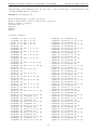
Example 3.5. The language bias:
#modeo(assigned(var(day), var(time)), (positive)).
#modeo(1, type(var(day), var(time), const(course)), (positive)).
#modeo(1, var(day) != var(day)).
#constant(course, c2).
#weight(1).
#maxv(4).
#maxp(2).
specifies the search space:
:~
:~
:~
:~
:~
:~
:~
:~
:~
:~
:~
:~
:~
:~
:~
:~
:~
:~
:~
:~
:~
:~
:~
:~
:~
assigned(V0,
assigned(V0,
type(V0, V1,
type(V0, V1,
assigned(V0,
assigned(V0,
assigned(V0,
assigned(V0,
assigned(V0,
assigned(V2,
assigned(V0,
assigned(V2,
assigned(V0,
assigned(V2,
assigned(V0,
assigned(V2,
assigned(V0,
type(V0, V1,
assigned(V0,
type(V0, V1,
assigned(V0,
type(V0, V2,
assigned(V0,
type(V0, V2,
assigned(V0,
type(V2, V1,
assigned(V0,
type(V2, V1,
assigned(V0,
type(V2, V3,
assigned(V0,
type(V2, V3,
assigned(V0,
assigned(V0,
assigned(V0,
assigned(V0,
assigned(V0,
assigned(V3,
assigned(V0,
assigned(V3,
assigned(V0,
assigned(V3,
assigned(V0,
assigned(V3,
assigned(V0,
assigned(V2,
V1).[1@1, 1, V0, V1]
V1).[1@2, 2, V0, V1]
c2).[1@1, 3, V0, V1]
c2).[1@2, 4, V0, V1]
V1),
V2).[1@1, 5, V0, V1, V2]
V1),
V2).[1@2, 6, V0, V1, V2]
V1),
V1).[1@1, 7, V0, V1, V2]
V1),
V1).[1@2, 8, V0, V1, V2]
V1),
V3).[1@1, 9, V0, V1, V2, V3]
V1),
V3).[1@2, 10, V0, V1, V2, V3]
V1),
c2).[1@1, 11, V0, V1]
V1),
c2).[1@2, 12, V0, V1]
V1),
c2).[1@1, 13, V0, V1, V2]
V1),
c2).[1@2, 14, V0, V1, V2]
V1),
c2).[1@1, 15, V0, V1, V2]
V1),
c2).[1@2, 16, V0, V1, V2]
V1),
c2).[1@1, 17, V0, V1, V2, V3]
V1),
c2).[1@2, 18, V0, V1, V2, V3]
V1), assigned(V0, V2),
V3).[1@1, 19, V0, V1, V2, V3]
V1), assigned(V0, V2),
V3).[1@2, 20, V0, V1, V2, V3]
V1), assigned(V0, V2),
V1).[1@1, 21, V0, V1, V2, V3]
V1), assigned(V0, V2),
V1).[1@2, 22, V0, V1, V2, V3]
V1), assigned(V0, V2),
V2).[1@1, 23, V0, V1, V2, V3]
V1), assigned(V0, V2),
V2).[1@2, 24, V0, V1, V2, V3]
V1), assigned(V2, V1),
V3).[1@1, 25, V0, V1, V2, V3]
:~ assigned(V0,
assigned(V2,
:~ assigned(V0,
assigned(V3,
:~ assigned(V0,
assigned(V3,
:~ assigned(V0,
type(V0, V1,
:~ assigned(V0,
type(V0, V1,
:~ assigned(V0,
type(V0, V2,
:~ assigned(V0,
type(V0, V2,
:~ assigned(V0,
type(V0, V3,
:~ assigned(V0,
type(V0, V3,
:~ assigned(V0,
type(V3, V1,
:~ assigned(V0,
type(V3, V1,
:~ assigned(V0,
type(V3, V2,
:~ assigned(V0,
type(V3, V2,
:~ assigned(V0,
type(V0, V1,
:~ assigned(V0,
type(V0, V1,
:~ assigned(V0,
type(V0, V3,
:~ assigned(V0,
type(V0, V3,
:~ assigned(V0,
type(V2, V1,
:~ assigned(V0,
type(V2, V1,
:~ assigned(V0,
type(V2, V3,
:~ assigned(V0,
type(V2, V3,
:~ assigned(V0,
type(V3, V1,
:~ assigned(V0,
type(V3, V1,
13
V1), assigned(V2,
V3).[1@2, 26, V0,
V1), assigned(V2,
V1).[1@1, 27, V0,
V1), assigned(V2,
V1).[1@2, 28, V0,
V1), assigned(V0,
c2).[1@1, 29, V0,
V1), assigned(V0,
c2).[1@2, 30, V0,
V1), assigned(V0,
c2).[1@1, 31, V0,
V1), assigned(V0,
c2).[1@2, 32, V0,
V1), assigned(V0,
c2).[1@1, 33, V0,
V1), assigned(V0,
c2).[1@2, 34, V0,
V1), assigned(V0,
c2).[1@1, 35, V0,
V1), assigned(V0,
c2).[1@2, 36, V0,
V1), assigned(V0,
c2).[1@1, 37, V0,
V1), assigned(V0,
c2).[1@2, 38, V0,
V1), assigned(V2,
c2).[1@1, 39, V0,
V1), assigned(V2,
c2).[1@2, 40, V0,
V1), assigned(V2,
c2).[1@1, 41, V0,
V1), assigned(V2,
c2).[1@2, 42, V0,
V1), assigned(V2,
c2).[1@1, 43, V0,
V1), assigned(V2,
c2).[1@2, 44, V0,
V1), assigned(V2,
c2).[1@1, 45, V0,
V1), assigned(V2,
c2).[1@2, 46, V0,
V1), assigned(V2,
c2).[1@1, 47, V0,
V1), assigned(V2,
c2).[1@2, 48, V0,
V1),
V1, V2,
V1),
V1, V2,
V1),
V1, V2,
V2),
V1, V2]
V2),
V1, V2]
V2),
V1, V2]
V2),
V1, V2]
V2),
V1, V2,
V2),
V1, V2,
V2),
V1, V2,
V2),
V1, V2,
V2),
V1, V2,
V2),
V1, V2,
V1),
V1, V2]
V1),
V1, V2]
V1),
V1, V2,
V1),
V1, V2,
V1),
V1, V2]
V1),
V1, V2]
V1),
V1, V2,
V1),
V1, V2,
V1),
V1, V2,
V1),
V1, V2,
V3]
V3]
V3]
V3]
V3]
V3]
V3]
V3]
V3]
V3]
V3]
V3]
V3]
V3]
V3]
Inductive Learning of Answer Set Programs - User Manual
:~ assigned(V0,
type(V0, V1,
:~ assigned(V0,
type(V0, V1,
:~ assigned(V0,
type(V0, V3,
:~ assigned(V0,
type(V0, V3,
:~ assigned(V0,
type(V2, V1,
:~ assigned(V0,
type(V2, V1,
:~ assigned(V0,
type(V2, V3,
:~ assigned(V0,
type(V2, V3,
3.2
V1), assigned(V2,
c2).[1@1, 49, V0,
V1), assigned(V2,
c2).[1@2, 50, V0,
V1), assigned(V2,
c2).[1@1, 51, V0,
V1), assigned(V2,
c2).[1@2, 52, V0,
V1), assigned(V2,
c2).[1@1, 53, V0,
V1), assigned(V2,
c2).[1@2, 54, V0,
V1), assigned(V2,
c2).[1@1, 55, V0,
V1), assigned(V2,
c2).[1@2, 56, V0,
V3),
V1, V2,
V3),
V1, V2,
V3),
V1, V2,
V3),
V1, V2,
V3),
V1, V2,
V3),
V1, V2,
V3),
V1, V2,
V3),
V1, V2,
V3]
V3]
V3]
V3]
V3]
V3]
V3]
V3]
M. Law, A. Russo, K. Broda
:~ assigned(V0, V1), assigned(V2,
V0 != V2.[1@1, 57, V0, V1, V2]
:~ assigned(V0, V1), assigned(V2,
V0 != V2.[1@2, 58, V0, V1, V2]
:~ assigned(V0, V1), assigned(V2,
V0 != V2.[1@1, 59, V0, V1, V2,
:~ assigned(V0, V1), assigned(V2,
V0 != V2.[1@2, 60, V0, V1, V2,
:~ assigned(V0, V1), type(V2, V1,
V0 != V2.[1@1, 61, V0, V1, V2]
:~ assigned(V0, V1), type(V2, V1,
V0 != V2.[1@2, 62, V0, V1, V2]
:~ assigned(V0, V1), type(V2, V3,
V0 != V2.[1@1, 63, V0, V1, V2,
:~ assigned(V0, V1), type(V2, V3,
V0 != V2.[1@2, 64, V0, V1, V2,
V1),
V1),
V3),
V3]
V3),
V3]
c2),
c2),
c2),
V3]
c2),
V3]
Example Tasks
In this section, we give example learning tasks involving ordering examples encoded in ILASP. The first shows how
ILASP can be used to learn soft constraints in a simple scheduling problem and is motivated by the running example
in the paper [8]. Further examples may follow in later editions of this manual.
3.2.1
Scheduling
The following scheduling example task is motivated by the running example in the paper [8]. It shows how we can
learn preferences using ILASP2 in the setting of interview scheduling.
Example 3.6. Consider the following learning task describing an interview scheduling problem. There are 9 slots
to be assigned (3 each on 3 days) and each slot is for a candidate on one of two courses (c1 or c2).
slot(mon,1..3).
slot(tue,1..3).
slot(wed,1..3).
% Three slots each on Monday, Tuesday and Wednesday.
type(mon,1,c2).
type(mon,2,c1).
type(mon,3,c1).
type(tue,1,c1).
type(tue,2,c1).
type(tue,3,c2).
type(wed,1,c1).
type(wed,2,c2).
type(wed,3,c1).
% The following interview slots for c1 and c2 are to be assigned:
%
%
--------------------%
|
| Mon | Tue | Wed |
%
=====================
%
| 1 | c2 | c1 | c1 |
%
|---+-----+-----+-----|
%
| 2 | c1 | c1 | c2 |
%
|---+-----+-----+-----|
%
| 3 | c1 | c2 | c1 |
%
---------------------
0 { assigned(X, Y) } 1 :- slot(X, Y).
#modeo(assigned(var(day), var(time)), (positive)).
#modeo(1, type(var(day), var(time), const(course)), (positive)).
#modeo(1, var(day) != var(day)).
14
Inductive Learning of Answer Set Programs - User Manual
M. Law, A. Russo, K. Broda
#constant(course, c2).
#weight(1).
%
%
%
%
For each example, we show the corresponding partial timetable. "Yes" means
that the person was definitely assigned the slot; "No" means that the person
definitely was not assigned the slot; "?" meas that whether this slot was
assigned to this person is unknown.
#pos(pos1, {
assigned(mon,1)
}, { }).
%
%
%
%
%
%
%
%
%
--------------------|
| Mon | Tue | Wed |
=====================
| 1 | Yes | ? | ? |
|---+-----+-----+-----|
| 2 | ? | ? | ? |
|---+-----+-----+-----|
| 3 | ? | ? | ? |
---------------------
#pos(pos2, {
assigned(mon,3),
assigned(wed,1),
assigned(wed,3)
}, {
assigned(mon,1),
assigned(tue,3),
assigned(wed,2)
}).
%
%
%
%
%
%
%
%
%
--------------------|
| Mon | Tue | Wed |
=====================
| 1 | No | ? | Yes |
|---+-----+-----+-----|
| 2 | ? | ? | No |
|---+-----+-----+-----|
| 3 | Yes | No | Yes |
---------------------
#pos(pos3, {
assigned(mon,1),
assigned(wed,3)
}, {}).
%
%
%
%
%
%
%
%
%
--------------------|
| Mon | Tue | Wed |
=====================
| 1 | Yes | ? | ? |
|---+-----+-----+-----|
| 2 | ? | ? | ? |
|---+-----+-----+-----|
| 3 | ? | ? | Yes |
---------------------
#pos(pos4, {
assigned(mon,1),
assigned(mon,2),
assigned(mon,3)
}, {
assigned(tue,1),
assigned(tue,2),
assigned(tue,3),
assigned(wed,1),
assigned(wed,2),
assigned(wed,3)
}).
%
%
%
%
%
%
%
%
%
--------------------|
| Mon | Tue | Wed |
=====================
| 1 | Yes | Yes | Yes |
|---+-----+-----+-----|
| 2 | No | No | No |
|---+-----+-----+-----|
| 3 | No | No | No |
---------------------
#pos(pos5, {
assigned(mon,2),
assigned(mon,3)
},{
assigned(mon,1),
assigned(tue,1),
assigned(tue,2),
assigned(tue,3),
assigned(wed,1),
%
%
%
%
%
%
%
%
%
--------------------|
| Mon | Tue | Wed |
=====================
| 1 | No | Yes | Yes |
|---+-----+-----+-----|
| 2 | No | No | No |
|---+-----+-----+-----|
| 3 | No | No | No |
---------------------
15
Inductive Learning of Answer Set Programs - User Manual
M. Law, A. Russo, K. Broda
assigned(wed,2),
assigned(wed,3)
}).
#pos(pos6, {
assigned(mon,2),
assigned(tue,1)
},{
assigned(mon,1),
assigned(mon,3),
assigned(tue,2),
assigned(tue,3),
assigned(wed,1),
assigned(wed,2),
assigned(wed,3)
}).
%
%
%
%
%
%
%
%
%
--------------------|
| Mon | Tue | Wed |
=====================
| 1 | No | Yes | No |
|---+-----+-----+-----|
| 2 | Yes | No | No |
|---+-----+-----+-----|
| 3 | No | No | No |
---------------------
#cautious_ordering(pos4, pos3).
#cautious_ordering(pos2, pos1).
#cautious_ordering(pos2, pos3).
#brave_ordering(pos5, pos6).
#maxv(4).
#maxp(2).
As the positive examples are already covered by the background knowledge (and there are no negative examples),
there is no need to change the answer sets of this program. For this reason, we only need to learn weak constraints
which cover the brave and cautious orderings. When run with ILASP, this task produces the output:
:~ assigned(V0, V1), type(V0, V1, c2).[1@2, 1, V0, V1]
:~ assigned(V0, V1), assigned(V2, V3), V0 != V2.[1@1, 2, V0, V1, V2, V3]
Pre-processing
Solve time
Total
: 0.01s
: 0.801s
: 0.811s
The first, higher priority weak constraint says that this person would like to avoid having interview slots for the
course c2. The second, lower priority weak constraint says that the person would like to avoid pairs of slots which
occur on different days.
16
Inductive Learning of Answer Set Programs - User Manual
4
M. Law, A. Russo, K. Broda
Specifying Learning Tasks with Noise in ILASP
Most real data has some element of noise in it. The tasks specified so far assume noise free data and, as such, require
that all examples should be covered by any inductive solution.
In fact, ILASP does have a mechanism for dealing with noisy data. Any example (including ordering examples) can
be given a weight w (a positive integer) to indicate that this example might be noisy. The goal of ILASP without
noise is to search for an hypothesis H which covers all the examples such that |H| is minimal. Any example which
is not given a weight is considered noise-free and, as such, must be covered.
If we let W be the sum of the weights of examples which might be noisy and is not covered, then the goal of ILASP
is now to find an hypothesis which covers all the noise-free examples and minimises |H| + W .
These weights are specified in ILASP by giving example name@weight in place of the usual example name. If an
example has been treated as noisy by the inductive solution which ILASP has found then it will report: % Warning
example: ‘example name’ treated as noise.
4.1
Example: Noisy Sudoku
Recall the sudoku task from section 2.3.1. If we now assign weights to the examples then the hypothesis might
change as it might be more costly to cover an example than to pay the corresponding penaulty. Note that the
original hypothesis had length 26 with each of the constraints having length 3 and the choice rule having length 17.
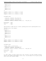
Example 4.1. If we set the weights as:
#pos(a@10, {
value((1, 1),
value((1, 2),
value((1, 3),
value((1, 4),
value((2, 3),
}, {
value((1, 1),
value((1, 1),
value((1, 1),
}).
1),
2),
3),
4),
2)
2),
3),
4)
#neg(b@10, { value((1, 1), 1), value((1, 3), 1) },{}).
#neg(c@10, { value((1, 1), 1), value((3, 1), 1) },{}).
#neg(d@10, { value((1, 1), 1), value((2, 2), 1) },{}).
then ILASP returns:
% Warning: example ‘a’ treated as noise.
Pre-processing
Solve time
Total
: 0.032s
: 0.135s
: 0.167s
This means that the optimal solution is to return the empty hypothesis. This covers the three negative examples
and so the only penaulty paid is 10 for the single positive example.
Example 4.2. If we set the weights as:
#pos(a@100, {
value((1, 1), 1),
value((1, 2), 2),
17
Inductive Learning of Answer Set Programs - User Manual
value((1,
value((1,
value((2,
}, {
value((1,
value((1,
value((1,
}).
M. Law, A. Russo, K. Broda
3), 3),
4), 4),
3), 2)
1), 2),
1), 3),
1), 4)
#neg(b@10, { value((1, 1), 1), value((1, 3), 1) },{}).
#neg(c@10, { value((1, 1), 1), value((3, 1), 1) },{}).
#neg(d@10, { value((1, 1), 1), value((2, 2), 1) },{}).
then ILASP returns:
:- value(V0,V1), value(V2,V1), same_col(V0, V2).
:- value(V0,V1), value(V2,V1), same_block(V2, V0).
:- value(V0,V1), value(V2,V1), same_row(V0, V2).
1 {value(V0,4); value(V0,3); value(V0,2); value(V0,1) } 1 :- same_row(V0, V1).
Pre-processing
Solve time
Total
: 0.027s
: 1.857s
: 1.884s
This means that the optimal solution is to return the optimal hypothesis from the original task (without noise).
Example 4.3. If we set the weights as:
#pos(a@100,
value((1,
value((1,
value((1,
value((1,
value((2,
}, {
value((1,
value((1,
value((1,
}).
{
1),
2),
3),
4),
3),
1),
2),
3),
4),
2)
1), 2),
1), 3),
1), 4)
#neg(b@1, { value((1, 1), 1), value((1, 3), 1) },{}).
#neg(c@4, { value((1, 1), 1), value((3, 1), 1) },{}).
#neg(d@4, { value((1, 1), 1), value((2, 2), 1) },{}).
then ILASP returns:
% Warning: example ‘b’ treated as noise.
:- value(V0,V1), value(V2,V1), same_block(V0, V2).
:- value(V0,V1), value(V2,V1), same_row(V2, V0).
1 {value(V0,4); value(V0,3); value(V0,2); value(V0,1) } 1 :- same_row(V0, V1).
Pre-processing
Solve time
Total
: 0.032s
: 3.191s
: 3.223s
Note that as examples c and d have weight 4 it is less costly to learn their corresponding constraints (of length 3);
whereas, because example b only has weight 1, it is less costly to treat this example as noise and pay the penaulty
than to learn an extra constraint of length 3.
18
Inductive Learning of Answer Set Programs - User Manual
5
M. Law, A. Russo, K. Broda
Hypothesis length
When specifying the search space in full you must also specify the length of each rule. This length is used to determine
the length of each hypothesis. The goal of ILASP is to search for an inductive solution which minimises this length.
If you use mode declarations to specify your search space then ILASP will assign a length to each rule. Usually, the
length of a rule R (written |R|) is just the number of literals in the rule. The only exceptions to this are choice rules.
The aggregate in the head of a choice rule is not counted simply as the number of atoms it contains, as this tends to
(in our opinion unreasonably) favour learning hypotheses containing choice rules.
A counting aggregate l{h1 , . . . , hn }u has length
n×
u
X
n
Ci
i=l
The inuition behind this is that this is the length of the counting aggregate once it has been converted to disjunctive
normal form.
Example 5.1. The counting aggregate 1{p, q}2 represented in disjunctive normal form would be (p ∧ not q)∨
( not p ∧ q) ∨ (p ∧ q); so, this is counted as length 6 rather than just length 2.
In our opinion, and for the examples we have tried, this weighting of choice rules better reflects the added complexity
they bring to an hypothesis.
If you wish to use a our search space, but with a different measure of hypothesis length then our suggested solution
is to call ILASP with the option -s which will produce our search space with our weights. You can then edit the
weights and add the rules to the search space manually (omitting the original mode bias).
19
Inductive Learning of Answer Set Programs - User Manual
M. Law, A. Russo, K. Broda
References
[1] M. Law, A. Russo, K. Broda, The ILASP system for learning answer set programs, https://www.doc.ic.ac.
uk/~ml1909/ILASP (2015).
[2] S. Muggleton, Inductive logic programming, New generation computing 8 (4) (1991) 295–318.
[3] M. Gelfond, V. Lifschitz, The stable model semantics for logic programming., in: ICLP/SLP, Vol. 88, 1988, pp.
1070–1080.
[4] C. Sakama, K. Inoue, Brave induction: a logical framework for learning from incomplete information, Machine
Learning 76 (1) (2009) 3–35.
[5] D. Corapi, A. Russo, E. Lupu, Inductive logic programming in answer set programming, in: Inductive Logic
Programming, Springer, 2012, pp. 91–97.
[6] O. Ray, Nonmonotonic abductive inductive learning, Journal of Applied Logic 7 (3) (2009) 329–340.
[7] M. Law, A. Russo, K. Broda, Inductive learning of answer set programs, in: Logics in Artificial Intelligence
(JELIA 2014), Springer, 2014.
[8] M. Law, A. Russo, K. Broda, Learning weak constraints in answer set programming, in: To be presented at
ICLP 2015. Currently under consideration for publication in TPLP., 2015.
[9] C. Baral, Knowledge Representation, Reasoning, and Declarative Problem Solving, Cambridge University Press,
New York, NY, USA, 2003.
[10] M. Gelfond, Y. Kahl, Knowledge Representation, Reasoning, and the Design of Intelligent Agents: The AnswerSet Programming Approach, Cambridge University Press, 2014.
[11] M. Gebser, R. Kaminski, B. Kaufmann, M. Ostrowski, T. Schaub, S. Thiele, A users guide to gringo, clasp,
clingo, and iclingo (2008).
[12] M. Law, A. Russo, K. Broda, Simplified reduct for choice rules in ASP., Tech. Rep. DTR2015-2, Imperial College
of Science, Technology and Medicine, Department of Computing (2015).
[13] M. Gebser, R. Kaminski, B. Kaufmann, M. Ostrowski, T. Schaub, M. Schneider, Potassco: The Potsdam answer
set solving collection, AI Communications 24 (2) (2011) 107–124.
20