Download VarEMU: An Emulation Testbed for Variability-Aware

VarEMU: An Emulation Testbed for
Variability-Aware Software
Lucas Wanner, Salma Elmalaki, Liangzhen Lai, Puneet Gupta, and Mani Srivastava
University of California, Los Angeles
{wanner, selmalaki, liangzhen, mbs}@ucla.edu, [email protected]
ABSTRACT
1.
Modern integrated circuits, fabricated in nanometer technologies, suffer from significant power/performance variation across-chip, chip-to-chip and over time due to aging
and ambient fluctuations. Furthermore, several existing and
emerging reliability loss mechanisms have caused increased
transient, intermittent and permanent failure rates. While
this variability has been typically addressed by process, device and circuit designers, there has been a recent push
towards sensing and adapting to variability in the various
layers of software. Current hardware platforms, however,
typically lack variability sensing capabilities. Even if sensing capabilities were available, evaluating variability-aware
software techniques across a significant number of hardware
samples would prove exceedingly costly and time consuming.
We introduce VarEMU, an extension to the QEMU virtual
machine monitor that serves as a framework for the evaluation of variability-aware software techniques. VarEMU provides users with the means to emulate variations in power
consumption and in fault characteristics and to sense and
adapt to these variations in software. Through the use (and
dynamic change) of parameters in a power model, users can
create virtual machines that feature both static and dynamic
variations in power consumption. Faults may be injected
before or after, or completely replace the execution of any
instruction. Power consumption and susceptibility to faults
are also subject to dynamic change according to an aging
model. A software stack for VarEMU features precise control over faults and provides virtual energy monitors to the
operating system and processes. This allows users to precisely quantify and evaluate the effects of variations on individual applications. We show how VarEMU tracks energy
consumption according to variation-aware power and aging
models and give examples of how it may be used to quantify
how faults in instruction execution affect applications.
The scaling of semiconductor processes to atomic dimensions has led to decreased control over manufacturing quality, which makes integrated circuit designs unpredictable.
This is compounded with aging related wear-out and environmental factors, and has led to fluctuations in critical
device/circuit parameters of manufactured parts across the
die, between dies, and over time. Consequently, electronic
devices are increasingly plagued by variability in performance (speed, power) and error characteristics across nominally identical instances of a part, and across their usage
life [14]. Variability has been typically isolated from software, and handled (or hidden, through guardbanding) by
process, device and circuit designers, which has led to decreased chip yields and increased costs [16].
Recently there have been several efforts to handle variability at higher system layers, including various layers of
software. The range of actions that the software can take
in response to variability includes: alter the computational
load by adjusting task activation; use a different set of hardware resources (e.g., use instructions that avoid a faulty
module or minimize use of a power hungry module); change
software parameters or the hardware’s operational setting
(e.g., tune software-controllable knobs such as voltage/frequency); and change the code that performs a task, either by
dynamic recompilation or through algorithmic choice. Concrete examples of variability-aware software include video
codec adaptation [23], embedded sensor deployment strategies [22, 12], duty cycling [32], memory allocation [1], procedure hopping [27], and error tolerant applications [9].
The evaluation of a variability-aware software stack faces
two main challenges: first, commercially available platforms
typically do not provide means to “sense” or discover variability. Second, even if this sensing capability was available,
evaluating a software stack across a statistically significant
number of hardware samples and ambient conditions would
prove exceedingly costly and time consuming.
In hardware design, simulations at various levels of abstraction can be used to evaluate the impacts of hardware
variability due to PVT (Process, Voltage, and Temperature) variations and circuit aging. While gate- and RTLlevel simulators can co-simulate both software and hardware, their runtimes are orders of magnitude slower than
real-time [7]. Cycle-accurate architecture-level simulators
like Wattch [4] suffer from the same problem. FPGA-based
emulators like [19, 9] can achieve similar runtime as realtime, but offer limited observability and controllability, and
suffer from poor portability and flexibility.
INTRODUCTION
In this paper we introduce VarEMU, an extensible framework for the evaluation of variability-aware software. VarEMU
provides users with the means to emulate variations in power
consumption and fault characteristics and to sense and adapt
to these variations in software. VarEMU is an extension to
the QEMU virtual machine monitor [25], which relies on
dynamic binary translation and supports a variety of target
architectures with very good performance. For many target
machines, QEMU provides faster than real time emulation.
Because QEMU can run unmodified binary images of physical machines, VarEMU enables the evaluation of complete
software stacks, with operating system, drivers, and applications.
In VarEMU, timing and cycle count information is extracted from the code being emulated. This information is
fed into a variability model, which takes configurable parameters to determine energy consumption and fault variations
in the virtual machine. Energy consumption and susceptibility to faults are also subject to dynamic change according
to an aging model. Control over faults and virtual energy
sensors are exported as “variability registers” mapped into
memory that is accessible to the software being emulated,
closing the loop. This information is exposed through a variability driver in the operating system, which can be used
to support software adaptation policies. Through the use
of different variability emulation parameters that capture
instance-to-instance, environmental, and age-related variation, VarEMU allows users to evaluate variability-aware software adaptation strategies across a statistically significant
number of hardware samples and scenarios.
The remainder of this paper is organized as follows. Section 2 presents related work. Section 3 presents the VarEMU
architecture, its variability models and details about their
implementation. Section 4 presents the software interfaces
from VarEMU to emulated software and external monitors
and users. Section 5 presents verification results and case
studies with VarEMU. Section 6 presents our conclusions.
2.
RELATED WORK
The hardware and software co-evaluation of variability effects can be done with instrumented hardware platforms or
simulations at various levels of abstraction. For example,
Wanner et. al. [32] used off-the-shelf hardware platforms
instrumented with power sensors to evaluate the impacts
of power variations on software duty-cycling. FPGA-based
platforms or architectural simulators can be used to evaluate system performance due to delay variations [19, 13] or
to inject hardware faults [9, 20, 24, 10]. Architectural simulators are typically several orders of magnitude slower than
real time. FPGA-based emulators can achieve fast runtime,
but offer limited observability and controllability, and suffer
from poor portability and flexibility.
Full system emulators can run unmodified binary code for
their target architectures. QEMU, on top of which VarEMU
was built, uses binary translation to achieve very good full
system emulation performance. Wind River Simics [28] is
a commercial simulator that features fault injections that
can change the contents of memory, registers, sensor readings, or network packets. While VarEMU currently does
not provide a high level mechanism for injection of faults in
sensor readings or network packets, it features a more powerful fault injection mechanism that allows arbitrary functions
that can manipulate virtual hardware state to be injected as
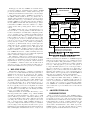
Virtual Machine
App
read energy
& cycle registers
App
enable / disable
faults
VarEMU Driver
OS
VarEMU
Instruction
disassembly
& translation
Virtual
Hardware
Device
Cycle & Time
Accounting
Energy
Accounting
Fault
Model
User I/O
Aging
Model
Power Model
Configure instruction classes
Change power model parameters
Query energy & cycle information
Software Monitor
User
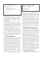
Figure 1: VarEMU Architecture
faults in any instruction. Furthermore, VarEMU integrates
fault injection with aging and power consumption models
not present in Simics. The gem5 simulator [3] has been extended to provide energy evaluation for parallel computing
loads [15]. Although gem5 is open source and capable of
booting a full Linux system for some of its target architectures, its performance is considerably worse than that of
QEMU [3]. Cycle-accurate architecture-level simulators like
Wattch [4] have runtimes of 2-3 orders of magnitude slower
than real-time, and are typically less robust than QEMU in
their support for running complete virtual machines.
Binary instrumentation tools such as Pin [21] could be
used to implement similar functionality to VarEMU, e.g.,
by inserting a callback to a variability module after the execution of every instruction. Binary instrumentation, however, typically does not support cross-architecture simulation. VarEMU also benefits from QEMU’s virtual hardware
device architecture to provide virtual sensors for the OS and
applications.
3.
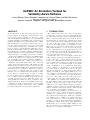
ARCHITECTURE AND
IMPLEMENTATION
Figure 1 presents an overview of the VarEMU architecture. Applications in a virtual machine interact with VarEMU
by querying for energy, cycle count, and execution registers
for different classes of instructions and by allowing or disallowing faults in the execution of emulated instructions. An
operating system driver mediates the interaction of applications with a virtual hardware device which exposes the
VarEMU interface to the VM. On VMs without operating
systems, applications handle this interaction directly.
When starting VarEMU, users provide a configuration file
that sorts instructions into different classes and parameters
to a model that is used to determine power consumption for
each of the classes. These parameters are subject to dynamic
change during runtime according to an aging model. Users
may change parameters for the power model dynamically
(e.g. to emulate variations in power consumption due to
changes in temperature, the user would periodically change
the temperature parameter of the power model). Users may
also query the VM’s cycle counters and energy registers.
Whenever an instruction is executed in the virtual machine, the cycle counter for its instruction class is incremented. Energy expenditure for a class of instruction is
determined as a function of accumulated execution time for
all instructions in that class and power consumption for the
class as determined by a power model.
For instructions configured by the user as susceptible to
faults, the execution of translated code may be preceded,
succeed, or replaced with alternative, faulty operations. These
operations may, in turn, cause changes to cycle counting
(e.g. due to a less precise version of the instruction taking fewer cycles to complete) or change parameters in the
power model (e.g. voltage or frequency). Faults are injected
only when explicitly activated by emulated software. A runtime parameter passed from emulated software to the fault
module when enabling faults allows users to configure which
faults are enabled and/or the nature of faults (e.g. precision of a numerical operation). This allows users to study
the effects of faults in instruction execution on individual
applications phases, without compromising the stability of
the runtime system. The remainder of this section describes
the architecture and implementation of VarEMU.
3.1
Cycle and Time Accounting
We account time in VarEMU on an instruction class basis.
Each instruction is associated with a user-defined class. A
data structure holds total number of cycles and time spent
executing instructions of each class. To associate instructions with classes, each instruction in a translation block is
augmented with an information structure (vemu_instr_info)
containing fields for the instruction operation code (opcode),
instruction name, instruction class, number of cycles, fault
status, and the instruction word itself.
When a new instruction word is found, its opcode is decoded, and the instruction information structure is filled
with its corresponding default values. An input file in JSON
format allows users to change the default number of cycles,
class, and fault status for any instruction. The number of
cycles may also be altered by the fault module at runtime.
A helper function in QEMU allows calling arbitrary functions from translated code. We use one such helper to perform a call to a function that increments the number of
cycles for a given instruction class after each instruction
is executed (vemu_increment_cycles). This function adds
the number of cycles in the instruction’s information structure to the total number of cycles for its instruction class.
Likewise, it increments total active time for that instruction
class, based on current (virtual) frequency. In processors
where the number of cycles taken by an instruction is not
constant, information from the instruction word (e.g. input
registers used, immediate values) could be used to accurately
determine the number of cycles.
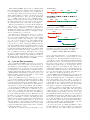
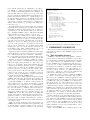
We must also account for cycles spent in standby or sleep
Hardware timing:
Active
WFI
Sleep
50 M Cycles
IRQ
0.5 s
Emulation timing:
Active
WFI
Sleep
50 M Cycles
IRQ
?
1 second
(a) Problem: emulation runs as best-effort, so execution and sleep times do not match hardware.
Active
Accounted: cycles/f
Emulation
WFI
Sleep
Emulation
IRQ
δ
Accounted
Time
(b) Solution: keep track of accounted and actual execution times, adjust sleep time interval accordingly.
Figure 2: Sleep Time Accounting
modes. In many architectures, a special instruction (e.g.
WFI in ARM, or HLT in x86 processors) puts the processor
in standby mode. After this instruction is issued, the processor will not execute other instructions until an interrupt
(typically from a timer or an external device) is fired. Keeping track of real sleep time (i.e., reflecting hardware timing)
is important for applications (e.g., in energy-aware duty cycling), as well as for circuit aging models. When we encounter such an instruction, we store a timestamp with current VM time. When an interrupt occurs following standby
we read a new timestamp, and add the time difference to
the counter for total time spent in sleep mode.
Because QEMU runs virtual machines as best-effort, the
actual execution frequency of emulated instructions may not
match the (virtual) frequency of the hardware. If the VM
never enters standby mode, there will be no adverse effects other than a discrepancy between total virtual time accounted with the cycle counters and wall clock time elapsed.
If the VM does enter a standby mode, time spent in that
mode must be adjusted to reflect hardware behavior.
Consider, for example, a system with periodic tasks where
processor utilization is less than 100%. After the system
completes tasks, it goes into standby mode, and waits for
a timer interrupt corresponding to the next period. Figure 2(a) illustrates such a system, where processor frequency
is 100 MHz, timer frequency is 1 Hz, task execution takes 50
M cycles (0.5 seconds), and time spent in standby mode is
0.5 seconds. If emulated execution is faster than hardware,
sleep time in the VM would be greater than in hardware.
Conversely, if emulation is slower than hardware, sleep time
in the VM would be smaller than in hardware.
In order for sleep time accounting in VarEMU to reflect
hardware timing, we keep track of emulated execution time
for each active time cycle. When a sleep cycle is initiated,
we calculate the delta between virtual execution time (from
our cycle counters, reflecting hardware execution time) and
emulated execution time for the last active period. We then
deduct this delta from the sleep time interval. Figure 2(b)
illustrates our solution. In cases where processor utilization
in hardware is 100%, but emulated execution time is faster
than hardware, it is possible for the sleep time interval to be
negative. In this case, the hardware version of the processor would continue executing immediately after the standby
instruction. We emulate this by returning a sleep interval
of 0. The converse situation (emulated time is slower than
virtual time) does not lead to a problem, as after continuing execution immediately after the standby instruction we
deduct a negative delta from an interval of zero, leading to
the correct positive sleep time interval.
3.2
Energy Accounting
Energy consumed by an instruction of a given class is determined as a function of execution time (number of cycles
divided by frequency) and power for that class. Power is
in turn determined by a model with arbitrary parameters
(minimally, voltage and frequency). By fitting the power
model with different parameters, users can emulate instanceto-instance variation. By changing parameters dynamically,
users can emulate the effects of dynamic or environmental
variation (e.g. due to changes in supply voltage or temperature). Power model parameters may also be dynamically
changed with an aging model.
While active and sleep time are accounted on a per-event
basis (i.e. on each instruction or sleep cycle), energy is accounted on demand, i.e. only when a read command is issued
from emulated software or external monitor, or when one of
the power model parameters change. For each energy accounting event, we keep track of sleep time and active time
for each class of instructions since the last event, and accumulate energy for each interval in the appropriate energy
registers. There is one active energy register per instruction
class, and one energy register for sleep energy.
Energy accounting is independent of power model, so that
users may define their own models. A power model implements three functions: The first function returns active
power in Watts for a given class of instruction. The second returns sleep power in Watts as a function of standby
mode (e.g. clock gated, power gated). The final function is
used to change power model parameter n of class c to value
v. Any power model must also define at least two parameters: frequency and voltage. The default power model for
VarEMU, presented in Section 3.4 defines several additional
parameters to capture static and dynamic variability.
3.3
NBTI Aging Model
Negative bias temperature instability (NBTI) is a circuit
wear-out mechanism that will degrade the PMOS threshold
voltage (Vthp ) and thus the circuit performance. To model
the NBTI-induced aging effect in VarEMU, we use the analytical model for the |Vthp | degradation of a MOS transistor
as in [8, 2, 31].
!2n
√ 2
Kv Tclk ω
|∆Vthp | =
1/2n
1 − βt
p
(1)
b1 + b2 (1 − ω)Tclk exp(b5 /T )
√
βt = 1 −
b3 + b4 t
Kv = b4 (Vdd − Vthp )exp(b5 /T )
where Vdd is the supply voltage, b1 , b2 , b3 , b4 , b5 are technologydependent parameters. Tclk is the time period of one stressrecovery cycle, ω is the duty cycle (the ratio of the time
spent in stress to time period), t is the total lifetime of a
transistor, n is a time exponent equal to 1/6 for an H2 diffusion model. Since NBTI-induced degradation is insensitive
to the switching frequency when it is larger than 100Hz [2],
similar to [31], we assume Tclk = 0.01s in this work.
Based on the aging model in (1), the key activity-related
parameters are the duty cycle ω and total lifetime t. In
VarEMU, we use the cycle counting feature to implement
the bookkeeping function for activity-related parameters,
i.e. total normal runtime tn and total runtime under power
gating tpg .
Since NBTI-induced degradation depends on the exact
signal switching pattern, VarEMU reports the upper and
lower bound aging scenarios. The upper bound of the aging scenario will be t = tn + tpg and ω = tn /t. The lower
bound of the aging scenario will be t = tn + tpg and ω =
0.5tn /t. Since the model in (1) assumes a periodic stressrecovery pattern, this model may not be adequate to accurately capture NBTI effects under some dynamical scenarios like dynamic voltage scaling and long-term power-gating.
To enable the dynamical features, it will require either more
sophiscated aging models (currently unavailable) or aging
simulators as in [6] (too slow for our purpose).
3.4
Aging-aware Power and Delay Model
In this section we present the default power model for
VarEMU which accounts for aging effects. The processor
power consumption can be classified as active power and
sleep power. Active power includes switching power and
short circuit power. In VarEMU, we use the switching power
model as in [26]:
Pswitching =
n
X
2
Ci βi Vdd
f
(2)
i=1
where Ci is the equivalent switching capacitance for each
instruction class i, βi is the fraction of class i instructions
in all instructions, and f is the clock frequency.
We use the short circuit power model as in [30]:
Pshort =
n
X
ηi (Vdd − Vthn − Vthp )3 f
(3)
i=1
where ηi is a technology- and design-dependent parameter for instruction class i, Vthn is the threshold voltage for
NMOS, and Vthp is the threshold voltage for PMOS and
equals |Vthp0 + ∆Vthp |, Vthp0 is the threshold voltage without degradation.
The sleep power can be modeled as:
Psleep = Vdd (Isub + Ig )
(4)
where Isub is the subthrshold leakage current and Ig is the
gate leakage current.
The leakage current models can be derived from the device model in [5]. We simplify the model and extract the
temperature- and voltage-dependency as:
−a2 Vthn
−a3 Vdd
−a2 Vthp
) + exp(
))exp(
)
T
T
T
(5)
where a1 , a2 , a3 are empirical fitted parameters.
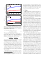
Isub = a1 T 2 (exp(
0.04
0.03
Delta Vt (V)
expect their sensitivity to voltage and temperature to follow
similar trends if the inverter chain is designed to match the
same design properties (e.g., cell types, fan-out ratio) of a
particular processor design. In this work, the final power and
delay values are normalized to the measured data obtained
from a Cortex M3 testchip using the same technology.
ref 0.8V
ref 1V
ref 1.2V
model 0.8V
model 1V
model 1.2V
0.035
0.025
0.02
3.5
0.015
0.01
0.005
0
0
0.04
1e+07
1.5e+07
Time (s)
2e+07
2.5e+07
3e+07
1e+07
1.5e+07
Time (s)
2e+07
2.5e+07
3e+07
ref 20C
ref 60C
ref 100C
model 20C
model 60C
model 100C
0.035
0.03
Delta Vt (V)
5e+06
0.025
0.02
0.015
0.01
0.005
0
0
5e+06
Figure 3: Threshold voltage degradation obtained
from reference design manual vs. fitted model in (1)
under different supply voltages at 60◦ C (top) and
temperatures at 1V(bottom)
We use the gate leakage model from [18]:
2
Ig = a4 Vdd
exp(−a5 /Vdd )
(6)
1
where a4 , a5 are empirical fitted parameters.
The dependence of circuit delay d on supply voltage Vdd
and threshold voltage can be modeled by the alpha-power
law [29]. Since NBTI has effect only on PMOS (PBTI on
NMOS respectively), due to the complementary property of
CMOS, the overall circuit delay can be modeled as:
Kp Cp Vdd
Kn Cn Vdd
d=
+
(7)
(Vdd − Vthp )α
(Vdd − Vthn )α
where Cp and Cn are equivalent load capacitances for PMOS
and NMOS respectively, Kp , Kn and α (1 < α < 2)) are
technology and design dependent constants.
In this work, we use a commercial 45nm process technology and libraries as our baseline. The aging model is
fitted to the NBTI aging equation given in the technology
design manual. The fitting results for different voltage and
temperature are shown in Figure 3. The power and delay
model parameters are fitted to the SPICE simulation results
of a inverter chain using device model given in the technology libraries. Compared to the power and delay value reported by SPICE results, errors in our model are less than
2% for 0.8V < Vdd < 1V , 0mV < |∆Vthp | < 50mV and
10◦ C < T < 90◦ C.
Although the absolute power and delay values of the entire
processor may not match the results of the inverter chain, we
1
There are secondary effects of temperature on some parameters such as threshold votage and electron mobility, but the
effects are neglagible for our purpose.
Faults
VarEMU allows faults to be inserted before or after, or
to completely replace the execution of an instruction. A
faulty implementation of an instruction in VarEMU is an arbitrary C function that has access to the complete architectural state of the VM, and hence may manipulate memory,
general purpose registers, and status and control registers.
Faulty versions of instructions may co-exist with its respective correct versions, and faults may be dynamically enabled
and disabled from emulated software.
When an instruction is disassembled, we check its VarEMU
field to determine if it is susceptible to faults. For instructions with pre and post execution faults, we simply generate code that calls the respective fault helper functions at
execution time. These helper functions determine whether
the fault will occur, and conditionally call the fault implementation. For instructions with replace faults, the code
generation process is more complex: if we simply called
a replace helper, the developer of the replacement fault
would also have to implement a correct version of the instruction. Hence, we generate two code paths, one for the
faulty path, and one for the original instruction (for when
faults do not occur). The faulty path is always called, and
returns a boolean value which determines whether the original instruction should be executed or not. This is accomplished with the equivalent of a conditional branch instruction, which jumps to the end of the current translation block
if the return value of the replace helper is not zero.
All of the following conditions must be met in order for a
fault to occur: 1) the instruction under execution is marked
as subject to faults; 2) the processor is not in a privileged
mode (e.g., faults are not permitted in the OS kernel); 3)
faults have been enabled by emulated software; 4) userdefined conditions, e.g., based on conditional or random variables. If these conditions are not met, the original version
of the instruction will be executed without faults.
Figure 4 shows a simple example of a stuck-at fault in the
multiply instruction. If the processor is currently running in
privileged mode, or if faults have not been enabled from emulated software, the function returns zero, which causes the
original instruction to be executed. Otherwise, the instruction operation code is decoded. For the multiply opcode,
the source and target registers are decoded, and the multiply operation is augmented with the stuck-at-one fault. The
result is written into the destination register.
While the fault presented in Figure 4 is deterministic in
nature (a stuck-at-one in the LSB of the target register)
and occurrence (always happens when faults are enabled in
non-privileged mode), users may include additional implementations or conditions for faults, e.g., based on history,
random variables, architectural state, or operational parameters such as voltage and frequency in the power model.
Users may also call external software modules (e.g. RTL
simulators) from the fault module in order to model realistic faults that, for example, take spacial correlation or instruction inter-dependency into account. Faulty execution
uint32_t vem u_f au l t _ r e p l a c e ( CPUArchState * env ,
TranslationBl oc k * tb )
{
if ( privmode |( v e m u _ f a u l t s _ e n a b l e d == 0) )
return 0;
switch ( instr_info - > opcode ) {
case OPCODE_MUL : {
int rd = ( instr_word >> 16) & 0 xf ;
int rs = ( instr_word >> 8) & 0 xf ;
int rm = ( instr_word ) & 0 xf ;
env - > regs [ rd ] = ( env - > regs [ rm ] * env - > regs [ rs ])
| 0 x01 ;
}; break ;
...
default : break ;
}
return 1;
}
Figure 4: Stuck-at fault in the multiply instruction
may in turn influence cycle counting (e.g. a faulty version
of an instruction that finishes in fewer cycles) or energy accounting (e.g. a faulty version of the instruction that is less
power intensive). Section 5 shows a small case study that
illustrates the usage of the VarEMU fault framework.
3.6
Portability
We currently support the ARM architecture (with Thumb
and Thumb2 extensions) in VarEMU. We’ve tested VarEMU
with two target machines: versatilepb (ARMv7) and lm3s6965
(Cortex-M3). Extending support to new target machines in
the same architecture is trivial: all that is needed is to map
the VarEMU virtual hardware device to a free slot in the
target machine’s address space and, if necessary, to adjust
the number of cycles per instruction.
Most VarEMU modules (e.g., energy accounting, user I/O,
virtual hardware device) are architecture independent. Power
model coefficients are empirically fitted to match the nominal power consumption of target platforms. Architecture
and device dependent modules include cycle counting (requires decoding and mapping of the target architecture instructions), power, and aging models. Because the implementation of faults typically involves manipulating registers,
memory, or processor state, specific implementations of instruction faults are not portable.
4.
SOFTWARE INTERFACES
VarEMU allows users and external software to configure
instruction information (class of instruction, susceptibility
to faults), dynamically change power model parameters, and
query the VM for cycle, time, and energy information.
An input file in JSON format specifies instruction classes
and power model parameters for a VM. A class of instructions is defined by an index, a name and a list of instruction
names. By default, all instructions are linked to a single
catch-all class. Instructions not listed in the input file remain linked to the default class. A dictionary links each
instruction class with its respective list of power model parameters. A minimal input file includes only a list of power
model parameters for the catch-all instruction class. The
input file may also define lists of instructions susceptible to
each type of fault supported by VarEMU.
QEMU provides a monitor architecture for external interaction with the VM. This monitor listens for commands and
sends replies on an I/O device (e.g. stdio or a socket). We
extended this monitor to provide commands to query a VM’s
energy, cycle, and time information, and to dynamically
typedef struct {
uint64_t act_time [ M A X _ I N S T R _ C L A S S E S ];
uint64_t act_energy [ M A X _ I N S T R _ C L A S S E S ];
uint64_t cycles [ M A X _ I N S T R _ C L A S S E S ];
uint64_t total_act_time ;
uint64_t t ot a l_ a ct _ en e rg y ;
uint64_t total_cycles ;
uint64_t slp_time ;
uint64_t slp_energy ;
uint64_t fault_status ;
} vemu_regs ;
Figure 5: VarEMU register layout
change power model parameters. Inputs and responses to
and from the monitor are in JSON format. A query-energy
command returns accumulated energy for sleep mode and
for each instruction class. Similarly, a query-time command
returns accumulated execution and sleep times. Finally, a
change-model-param command allows users to change power
model parameter n of class c to value v.
A combination of the change-model-param command described above and the standard stop and cont commands
provided by QEMU allows users to systematically emulate
dynamic variations in power consumption due to environmental factors (e.g. changes in ambient temperature).
We implemented a small application that demonstrates
interaction with the VarEMU monitor commands. This application queries the monitor every second for energy and
time information and plots average active and sleep power
for that time interval. Inputs allow users to change the temperature in the power model, which leads to changes in average power consumption.
4.1
Interaction with Emulated Software
Emulated software interacts with VarEMU through memory mapped registers. A virtual hardware device maps I/O
operations in specific memory regions to VarEMU functions.
A command register provides three operations: read, enable
faults, and kill. The read operation creates a checkpoint
for all VarEMU registers (Figure 5). Subsequent reads to
register memory locations will return values from the last
checkpoint. This allows users to read values that are temporally consistent across multiple registers.
A write to the enable faults command register propagates
its input value to a variable shared with the VarEMU fault
module. A value of 0 means that faults are completely disabled. The implications of a write to the fault register with
a value greater than zero depend on the specific implementation of the fault model, but in general such a write means
that faults are allowed to happen from this point on.
Finally, a write to the kill command register kills the VM
and stops emulation. This allows users to systematically
finish an emulation session in machines that do not provide
the equivalent of a shutdown command.
In machines without an operating system (or memory protection), applications may directly interact with the VarEMU
memory region. We provide a small library of high level
functions that issues the adequate sequence of write/read
operations in order to interact with VarEMU. For machines
that use the Linux operating system, these operations are
embedded into a driver, which also performs per-process
time and energy accounting and handles fault status.
4.2
Software Interface for Linux
In a multi-process system, it is difficult to attribute energy expenditure to different processes from a global energy
meter without system support. Furthermore, it would be
very difficult to conduct experiments and evaluate the impact of faults to individual applications in a multi-process
system if fault states were allowed to cross process boundaries. For example, if enabling faults in an application led to
faults being enabled in kernel code, or in the shell process,
the system would most likely become unstable and/or crash.
Nevertheless, a multi-process system typically provides several software conveniences that may not be available in a
simpler, OS-less system (e.g. I/O shell, networking stack,
remote file copy).
We implemented a series of small extensions to the Linux
kernel that allows applications to benefit from its software
stack while avoiding the issues described above. First, we
extended the process data structure with a new data structure containing VarEMU registers. This field holds fault
status and time and energy counters for each process.
When a process is scheduled in, we create a checkpoint
by reading all VarEMU registers from hardware. When the
process is scheduled out, we create a second checkpoint. Energy and cycles between the schedule in and out events are
attributed to the process. Energy and cycles between the
out event for the previous process and the in event for the
next process are attributed to the operating system. Fault
status is part of process context, and hence saved/restored
in scheduling events. Thus, enabling faults in one process
does not enable faults in other processes or the OS.
Applications interact with the VarEMU driver through a
system call interface. A write system call takes two parameters: command and value. Two commands — which map to
the corresponding operations in the virtual hardware device
— are available: fault and kill. Value is ignored for the kill
command. A read system takes two parameters: an integer type and a pointer to a VarEMU data structure (which
mirrors the register layout in Figure 5). Type can be system, process, or hardware. Read system calls issue the read
command to the hardware hardware device, read VarEMU
registers, and copy values into the VarEMU data structure
provided by the user, according to the type variable. Type
can be system (reads counters for the OS), process (reads
counters for the current process), or hardware (reads raw
hardware counters). A small library of functions aids users
in the interaction with the VarEMU driver.
Figure 6 shows how a Linux application may interact with
VarEMU. The vemu_regs data structure holds fields for all
time, energy, cycle, and fault registers. The main function
goes through an infinite loop where it reads and prints out
energy values for process, system, and hardware. It then
enables faults and goes through a for loop with multiplication and additions. Until faults are disabled again towards
the end of the main loop, faults are allowed for this process. This means that, for every instruction configured as
susceptible to faults by the user, a call will be issued to the
VarEMU fault model. The exact nature of the faults will
depend on the fault model implementation and may lead to
application crashes (e.g. due to invalid pointers being computed as a result of a faulty add instruction). A fault or
crash in this application will not lead to faults in the kernel
or in other processes.
While our example application only reads and prints out
VarEMU register values, variability-aware applications could
use this information to adapt its quality of service based on
energy constraints. Likewise, extensions to the OS kernel
# include < stdio .h >
# include " vemu . h "
int main () {
vemu_regs hw , sys , proc ;
do {
usleep (1000000) ;
vemu_read ( READ_HW , & hw ) ;
vemu_read ( READ_SYS , & sys ) ;
vemu_read ( READ_PROC , & proc ) ;
printf ( " Energy : \ n " ) ;
printf ( " hw : % d sys : % u proc : % u sleep : % u \ n " ,
hw . total_act_energy ,
sys . total_act_energy ,
proc . total_act_energy ,
hw . slp_energy ) ;
int i , x , y , z , sum ;
v e m u _ e n a b l e _ f a u l t s (1) ;
for ( i = 0; i < 100; i ++) {
z = x * y;
sum = sum + z ;
}
v e m u _ d i s a b l e _ f a u l t s () ;
printf ( " sum : % d " , sum ) ;
} while (1) ;
}
Figure 6: Linux application using VarEMU
could use this information to inform scheduling decisions.
5.
EXPERIMENTS AND RESULTS
This section presents verification and performance results
along with case studies for the VarEMU aging model and
fault framework.
5.1
Time Accounting Accuracy
VarEMU accounts time on the basis of number of instructions executed, clock frequency, and number of cycles taken
by each instruction. In hardware implementations, the number of cycles taken by some instructions may be variable.
Because VarEMU relies on an underlying platform of functional (not cycle accurate) emulation, this variable timing
information is not available to our time accounting module,
and instructions are assumed to take a fixed number of cycles based on their operation code. While this number of
cycles may be calibrated to reflect specific platforms and
workloads, it is inherently subject to inaccuracy.
To quantify the accuracy of time accounting in VarEMU,
we compare execution times in hardware with execution
times reported by VarEMU for different applications. For
each application tested, we follow the same sequence of events:
1) a GPIO pin is raised, 2) a VarEMU read command is issued 3) the main body of the application is executed, 4)
the GPIO pin from step 1 is lowered, and 5) a new read
command is issued. Because both the GPIO write and the
VarEMU read command can be implemented with a single
“write” instruction (in systems without an OS), there is only
one instruction difference between the two. By connecting
the GPIO pin to an oscilloscope and measuring is logical
high period, we can quantify execution time in hardware.
For this evaluation, we used the LM36965 model CortexM3 processor by Texas Instruments. When running in hardware, interaction with VarEMU is replaced with equivalent
read/write operations in a reserved area in memory. GPIO
operations have no effect in QEMU, but are still accounted
for (i.e. a read or write instruction is executed). To check
against cumulative errors, we ran a varying number of iterations for each application.
Figure 7 shows VarEMU time accounting accuracy for dif-
App
Dhrystone
Whetstone
null syscall
context switch
dd if=/dev/zero
Bitmap to JPEG
WAV to MP3 (lame)
Unit
p/sec.
MIPS
µs
µs
s
s
s
Vanilla QEMU
259304
14.2
12.4
61
0.98
0.9
19.1
VarEMU
102536
5
13.5
75.6
1.43
1.3
57.3
Overhead
150%
180%
9%
24%
46 %
45 %
200 %
Kernel
98352
4.8
13.5
88.3
1.49
1.31
57.4
Overhead
4%
4%
0%
17 %
2%
1%
0%
Total Overhead
164 %
196 %
9%
45 %
49 %
46 %
200 %
Table 1: Runtime overheads for VarEMU and the VarEMU kernel extensions
head. Because VarEMU adds a function call with constant
execution time to each instruction, for very efficient instructions the VarEMU extensions become a significant part of
total execution time. For less efficient instructions, VarEMU
overhead is relatively smaller. For our test applications,
best-case overhead was 9%, and worst-case 200%.
The overhead of the Linux kernel extensions for VarEMU
also depends on workload. Bookkeeping is performed for
every process switch, and therefore the context switch operation has the highest overhead, at 17%. For the other
applications in our test set, the overhead is at most 4%.
Total combined overhead for VarEMU, including emulation
Figure 7: Time Accounting Accuracy
and kernel overheads, ranged from 9% to 200% for our test
applications. Since QEMU (in combination with a fast host
ferent applications. Accuracy is defined as the ratio between
system) provides faster than real-time emulation for many of
actual execution time in hardware and execution time reits target platforms, this overhead is manageable, and much
ported by VarEMU. We calibrated the number of cycles per
smaller than that of other simulation alternatives such as
instruction using the “empty loop” application, and hence
cycle-accurate simulators. In future work, we intend to optithat application has the highest accuracy. For all other apmize the cycle counting module of VarEMU by replacing its
plications, accuracy is better than 96%, and does not incurrent implementation, which uses high-overhead QEMU
crease with longer execution runs. In future work, we intend
helper functions, with low-overhead intermediate interpreter
to increase this accuracy by performing deeper inspection of
instructions.
instruction words (e.g., in Cortex-M3 cores, some instructions take more or less cycles depending on which registers
are used), and by performing basic bookkeeping on branches
5.3 Case Study: Approximate Arithmetic
and load/store instructions to estimate pipeline bubbles.
In this section we present a small case study that uses the
VarEMU fault module to implement approximate arithmetic
5.2 Runtime Overheads
operations. Approximate arithmetic is used to increase the
Every time an emulated instruction is executed a call is
throughput of the application or reduce the consumed power
made to the VarEMU module that performs cycles and time
by reducing the cycle period or reducing the number of cyaccounting. Periodically, the cycle counting module makes
cles taken by each instruction. By propagating control over
calls to the aging module. If an instruction is susceptible
the hardware approximation to the software stack, we can
to errors, its translated code is augmented with calls to the
allow the software programmer to adaptively configure the
error module. Finally, every time a query is issued for the
approximate behavior at runtime based on the software reenergy counters, or whenever a variability model parameter
quirements. This shifts the power vs. performance or power
(e.g. temperature) changes, the power model is called.
vs. latency tradeoffs to a higher level which can lead to
On the emulated software system, the Linux module for
better solutions that vary from one application to another.
VarEMU performs per-process energy and time accounting.
The main bottleneck of most adders is the propagation
Every time a process is switched in or out, a read command
of the carry-chain. Bounds have been established for deis issued to the VarEMU virtual hardware module, and all
lay of reliable adder schemes, where no reliable adder can
VarEMU registers are copied. When an OS is not available,
have a sub-logarithmic delay [11]. However, unreliable
the standalone VarEMU library performs the same function.
adders could reach sub-logarithmic delay by cutting down
To quantify the various runtime overheads of VarEMU, we
the carry-chain. We adapted a configurable approximate
compare runtime performance of software under VarEMU
adder design [17] for an image edge filter application where
with its equivalent performance under the vanilla version
addition is done by concatenating a number of partial sums
of QEMU. We measured the relevant performance metrics
generated by an approximate adder. A faulty replacement
(e.g. time-to-completion, throughput) of various software
for add instructions was implemented as described in [17].
applications. Table 1 presents the resulting average of each
A parameter passed from emulated software to the VarEMU
application’s metric over 10 runs.
fault module when enabling faults is used to set the accuThe overhead of VarEMU over the vanilla version of QEMU
racy in the approximate add routine, where 25% accuracy
is highly dependent on workload. This is due to the fact
means 25% of the partial sums generated by the approxithat some emulated instructions (e.g. integer arithmetic)
mate adder are being corrected to give accurate partial sums.
translate very efficiently into native instructions, while othWe used approximate calculation for the value of each pixel
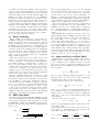
ers (e.g., load/stores, branches) have higher emulation overduring edge filtering. Depending on the micro-architecture
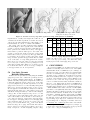
(a) Original Image.
(b) Accurate Edge Filter.
(c) Edge Filter with Approximate Adder
Using 25% Accuracy Correction.
Figure 8: Variable accuracy edge filter application using fault injection in VarEMU
implementation, a faulty adder might affect different sets
of instructions. In this experiment, we assume the adder is
only used by the ALU add instruction. Other faults, e.g. in
branch instructions, can also be emulated in VarEMU.
The output of the edge filter application under VarEMU
is shown in Figure 8, where 8(b) shows the result with the
accurate operations, and 8(c) shows the result with approximate operations. We evaluated the accuracy of the approximate addition operations with respect to the result of the
accurate operations and obtained a pass rate of 96%, which
matches the accuracy reported in [17]. The approximate filter accurately detected 99.8% of black edges in the original
image, and 97% of pixels in the approximate filter are within
± 5% of the value of corresponding pixels in the accurate
filter. As per [17], clock period may be reduced by 25% with
6% recovery-cycle overhead (correction penalty) for 16 bit
adder using 4 partial sums. This led to a reduction of 18%
in execution time with no increase in energy consumption
for the approximate case in our experiment.
5.4
Case Study: Dynamic
Reliability Management
In this section, we present a case study using the VarEMU
aging and power model to evaluate the potential power savings of dynamic reliability managements. In VarEMU, a
dynamic reliability management is implemented which automatically adjusts the supply voltage based on the delay
reported by Equation (7). In this experiment, we use the
aging model as in Section 3.3. The reliability management
unit is set to increase the supply voltage by step of 5mV .
We run applications with different activity factors with the
management unit enabled (i.e. with adaptive voltage) and
without the management unit (i.e. with one-time margined
voltage). The one-time margined voltage is set to account
for the aging scenario with 100% software duty cycle and
100◦ C. The results are shown in Table 2, where DC is processor duty cycle (fraction of active time), T is temperature,
mode is upper bound aging (UB), lower bound aging (LB),
and non-adaptive (NA), PS and PA are average sleep and
active power across the lifetime, ∆Vthp is the total delta in
threshold voltage due to aging, and UP, LB, NA stand for
upper bound, lower bound and non-adaptive cases respectively. Compared to one-time margining, adaptive voltage
DC (%)
T(◦ C)
21
100
100
21
40
100
Mode
LB
UB
NA
LB
UB
NA
LB
UB
NA
LB
UB
NA
PS (uW)
92.71
92.72
108.85
315.12
315.12
360.56
90.85
91.15
107.2
300.14
297.97
340.1
PA (mW)
6.06
6.08
6.87
6.31
6.39
7.22
6.01
6.04
6.84
6.31
6.30
7.13
∆Vthp (mV)
7.10
13.38
15.38
18.92
35.67
41.00
5.88
6.75
7.75
15.69
17.97
20.66
Vdd
1.01
1.015
1.040
1.020
1.030
1.040
1.005
1.010
1.040
1.015
1.015
1.040
Table 2: Aging Experiment Results
scaling can achieve 11% to 13%2 active power saving and
11% to 15% sleep power saving. Note that these values
heavily depend on the actual aging and power model.
6.
CONCLUSIONS
We presented VarEMU, an extensible framework for the
evaluation of variability-aware software based on the QEMU
virtual machine monitor. VarEMU uses cycle counting to accurately keep track of execution times in a virtual machine
and relies on variability-aware power and aging models to
determine energy consumption. Its fault injection mechanism allows arbitrary functions to augment or replace the
execution of any instruction in the system. Emulated software has access to time and energy registers and precise
control over when and under what circumstances faults are
allowed to occur. Linux kernel extensions for VarEMU allow
users to precisely quantify the effects of power variations and
variability-driven fault injection to individual applications.
While VarEMU adds 9–200% overhead to baseline QEMU
performance, it is significantly faster than other variability
emulation alternatives, which are typically orders of magnitude slower than real-time. In future work, we will explore
performance optimizations in the critical paths of VarEMU
to reduce overhead. VarEMU currently tracks hardware timing with 96% accuracy. We intend to increase this accuracy
by performing deeper inspection of instruction words, and
by performing basic bookkeeping on branches and load/store instructions to estimate pipeline bubbles. We will vali2
2
The savings here are larger than implied by a simple Vdd
power model, because the short-circuit power is proportional
to (Vdd − Vthn − |Vthp |)3 as in Equation (3).
date these extensions along with our existing power models
with an M3 test platform instrumented for power analysis [33]. VarEMU currently supports the ARM architecture
(with Thumb/Thumb2 extensions). We intend to support
other architectures in the future, including OpenSparc and
OpenMIPS. Further, we will model delay variability induced
errors (e.g. due to timing speculation).
VarEMU, its supporting Linux kernel extensions, test applications, and virtual power monitor are available for download at http://github.com/nesl/varemu.
Acknowledgements
This material is based upon work supported by the NSF under awards # CNS-0905580 and CCF-1029030. Any opinions, findings and conclusions or recommendations expressed
in this material are those of the author(s) and do not necessarily reflect the views of the NSF. Lucas Wanner was supported in part by CAPES/Fulbright grant #1892/07-0. The
authors wish to thank Gauresh Rane, who coded the first
VarEMU prototype, and Paul Martin and Ankur Sharma,
who tested various versions of the software.
7.
REFERENCES
[1] Luis Angel D. Bathen, Mark Gottscho, Nikil Dutt, Alex
Nicolau, and Puneet Gupta. Vipzone: Os-level memory
variability-driven physical address zoning for energy
savings. In CODES+ISSS, 2012.
[2] S. Bhardwaj, Wenping Wang, R. Vattikonda, Yu Cao, and
S. Vrudhula. Predictive modeling of the NBTI effect for
reliable design. In CICC, 2006.
[3] N. Binkert, B. Beckmann, G. Black, S. Reinhardt, A. Saidi,
A. Basu, Joel Hestness, Derek R. Hower, T. Krishna,
S. Sardashti, R. Sen, K. Sewell, M. Shoaib, N. Vaish,
M. Hill, and D. Wood. The gem5 simulator. SIGARCH
Comput. Archit. News, 39(2):1–7, August 2011.
[4] David Brooks, Vivek Tiwari, and Margaret Martonosi.
Wattch: a framework for architectural-level power analysis
and optimizations. ACM SIGARCH Computer Architecture
News, 28(2):83–94, 2000.
[5] BSIM. BSIM user manual.
http://www-device.eecs.berkeley.edu/bsim/, 2013.
[6] Tuck-Boon Chan, John Sartori, Puneet Gupta, and Rakesh
Kumar. On the efficacy of NBTI mitigation techniques. In
DATE, 2011.
[7] Debapriya Chatterjee, Andrew DeOrio, and Valeria
Bertacco. Gcs: High-performance gate-level simulation with
GPGPUs. In DATE, 2009.
[8] Xiaoming Chen, Yu Wang, Yu Cao, Yuchun Ma, and
Huazhong Yang. Variation-aware supply voltage assignment
for simultaneous power and aging optimization. IEEE
TVLSI, 20(11):2143–2147, 2012.
[9] Hyungmin Cho, L. Leem, and S Mitra. Ersa: Error resilient
system architecture for probabilistic applications. IEEE
TCAD, 31(4):546–558, 2012.
[10] Pierluigi Civera, Luca Macchiarulo, Maurizio Rebaudengo,
Matteo Sonza Reorda, and Massimo Violante. FPGA-based
fault injection techniques for fast evaluation of fault
tolerance in VLSI circuits. In Proc. Intl. Conf. on
Field-Programmable Logic and Applications, 2001.
[11] Milos Ercegovac. Digital arithmetic. Morgan Kaufmann
Publishers, San Francisco, CA, 2004.
[12] Siddharth Garg and Diana Marculescu. On the impact of
manufacturing process variations on the lifetime of sensor
networks. In CODES+ISSS, 2007.
[13] Siddharth Garg and Diana Marculescu. System-level
throughput analysis for process variation aware multiple
voltage-frequency island designs. TODAES, 13(4):59, 2008.
[14] P. Gupta, Y. Agarwal, L. Dolecek, N. Dutt, R.K. Gupta,
R. Kumar, S. Mitra, A. Nicolau, T.S. Rosing, M.B.
Srivastava, S. Swanson, and D. Sylvester. Underdesigned
and opportunistic computing in presence of hardware
variability. IEEE TCAD, 32(1):8–23, 2013.
[15] M. Hsieh, K. Pedretti, J. Meng, A. Coskun,
M. Levenhagen, and A. Rodrigues. Sst + gem5 = a scalable
simulation infrastructure for high performance computing.
In ICST SIMUTOOLS, 2012.
[16] K. Jeong, A.B. Kahng, and K. Samadi. Impact of
Guardband Reduction On Design Outcomes: A Quant.
Approach. IEEE T. on Semiconductor Manufacturing,
22(4):552–565, 2009.
[17] A.B. Kahng and Seokhyeong Kang. Accuracy-configurable
adder for approximate arithmetic designs. In DAC, 2012.
[18] N. S. Kim, T. Austin, D Baauw, T Mudge, K Flautner, J S
Hu, M J Irwin, M Kandemir, and V Narayanan. Leakage
current: Moore’s law meets static power. Computer,
36(12):68–75, 2003.
[19] Vivek J Kozhikkottu, Rangharajan Venkatesan, Anand
Raghunathan, and Sujit Dey. Vespa: Variability emulation
for system-on-chip performance analysis. In DATE, 2011.
[20] Man-Lap Li, Pradeep Ramachandran, Swarup Kumar
Sahoo, Sarita V Adve, Vikram S Adve, and Yuanyuan
Zhou. Understanding the propagation of hard errors to
software and implications for resilient system design. ACM
Sigplan Notices, 43(3):265–276, 2008.
[21] Chi-Keung Luk, Robert Cohn, Robert Muth, Harish Patil,
Artur Klauser, Geoff Lowney, Steven Wallace, Vijay Janapa
Reddi, and Kim Hazelwood. Pin: building customized
program analysis tools with dynamic instrumentation.
SIGPLAN Not., 40(6):190–200, June 2005.
[22] T. Matsuda, T. Takeuchi, H. Yoshino, M. Ichien,
S. Mikami, H. Kawaguchi, C. Ohta, and M. Yoshimoto. A
power-variation model for sensor node and the impact
against life time of wireless sensor networks. In ICCE, 2006.
[23] A. Pant, P. Gupta, and M. Van der Schaar. Appadapt:
Opportunistic application adaptation in presence of
hardware variation. TVLSI, 20(11):1986–1996, 2012.
[24] Andrea Pellegrini, Robert Smolinski, Lei Chen, Xin Fu,
Siva Kumar Sastry Hari, Junhao Jiang, SV Adve, Todd
Austin, and Valeria Bertacco. Crashtest’ing swat:
Accurate, gate-level evaluation of symptom-based resiliency
solutions. In DATE, 2012.
[25] QEMU. QEMU open source processor emulator.
http://qemu.org, 2013.
[26] Jan M Rabaey, Anantha P Chandrakasan, and Borivoje
Nikolic. Digital integrated circuits, volume 996.
Prentice-Hall, 1996.
[27] Abbas Rahimi, Luca Benini, and Rajesh Gupta. Procedure
hopping: a low overhead solution to mitigate variability in
shared-l1 processor clusters. In ISLPED, 2012.
[28] Wind River. Simics.
http://www.windriver.com/products/simics/, 2013.
[29] Takayasu Sakurai and A Richard Newton. Alpha-power law
mosfet model and its applications to cmos inverter delay
and other formulas. IEEE J. of Solid-State Circuits,
25(2):584–594, 1990.
[30] Harry JM Veendrick. Short-circuit dissipation of static cmos
circuitry and its impact on the design of buffer circuits.
IEEE J. of Solid-State Circuits, 19(4):468–473, 1984.
[31] Wenping Wang, Shengqi Yang, Sarvesh Bhardwaj, Rakesh
Vattikonda, Sarma Vrudhula, Frank Liu, and Yu Cao. The
impact of nbti on the performance of combinational and
sequential circuits. In DAC, 2007.
[32] Lucas Wanner, Charwak Apte, Rahul Balani, Puneet
Gupta, and Mani Srivastava. Hardware variability-aware
duty cycling for embedded sensors. IEEE Transactions on
VLSI Systems, 21(6):1000–1012, 2013.
[33] Bing Zhang. A platform for variability characterization of
ARM cortex M3 processors. Master’s thesis, UCLA, 2012.