Download Autonomous Golf Cart

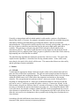
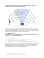
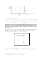
Autonomous Golf Cart
Drew Gaynor, Tyler Latham, Ian Anderson, and Cameron Johnson
Ohio Northern University, Ada, Ohio 45810
Email: [email protected]
1 – Abstract
As part of a multi-year senior design project at Ohio Northern University (ONU), a system has
been incrementally developed with the ultimate goal of autonomously transporting passengers to
and from locations within the ONU campus. While considering utility, safety, budget, and other
constraints, an autonomous system has been implemented using a standard electric golf cart
vehicle and various instruments used for positioning, obstacle avoidance, safety, navigation, and
otherwise as necessary. The project is still in active development, but as of the writing of this
paper, the system is capable of safely transporting passengers from one location to a nearby
destination in a relatively controlled environment.
2 – Problem Statement
Light transportation around areas such as university campuses is often needed for various
reasons including campus tours for prospective students, their families, or alumni. Passengers
are often transported to campus locations in golf carts run by human operators. An autonomous
system that would require minimal human interaction could eliminate the need for such human
operators and allow for an efficient method of transportation.
Such a system has several major requirements. It should:
Travel to a destination upon a user’s selection of that destination
o Select the best among the various routes to the chosen destination
o Accurately follow this planned path along campus roads and sidewalks
Require no other user input throughout the trip, except in the case of an emergency
Transport passengers with a reasonable degree of safety
o Avoid collisions with obstacles in the path to the destination
o Stop immediately upon collision with an obstacle
o Provide emergency stop buttons or other inputs to allow passengers to stop
operation of the vehicle immediately if needed
3 – System Architecture
An overview of the system architecture is show in Figure 1.
Proceedings of the 2013 ASEE North-Central Section Conference
Copyright © 2013, American Society for Engineering Education
Figure 1: Basic system block diagram
3.1 – Electrical
The electrical system of the golf cart is based on the factory-standard six 8-volt batteries wired in
series to provide a 48-volt power supply. This 48-volt supply is used directly to power the servo
used for rotating the steering column, the speed controller, and a DC-DC converter with an
output of 12 volts. The components on this 12-volt circuit are:
National Instruments (NI) CompactRIO (cRIO)
NI modules used with cRIO
OXTS inertial and GPS navigation system
Three of the batteries are also used in series to provide a 24-volt supply to several components:
Clutch electromagnet in steering assembly
Zippswitch safety impact sensor
LIDAR unit
3.2 – National Instruments CompactRIO
The NI CompactRIO 9022 real-time controller is used in this project for interfacing with almost
all elements of the system, including the laptop computer running Java software, GPS/INS unit,
Proceedings of the 2013 ASEE North-Central Section Conference
Copyright © 2013, American Society for Engineering Education
LIDAR sensor, steering system, speed controller, and other NI modules. It runs the LabVIEW
code that ties all of these elements together, as described in the following sections.
3.3 – Steering
The steering system utilizes the following components:
Servo motor and encoder
NI 9505 servo drive module
NI 9263 analog output module
NI CompactRIO 9022 real-time controller
Advanced Motion Controls (AMC) 25A8 servo drive
AMC FC10010 inductive filter card
Deltran SB-40B24-E08 electromagnetic clutch
Laptop computer
Through the steering input into the high-level Java application on the laptop computer, typically
via the path-following algorithms, a desired steering position is determined and transmitted to the
LabVIEW application running on the cRIO. Using this desired value and the current servo
position value transmitted from the servo encoder, the voltage to be applied to the servo is
determined. A voltage of up to ten volts is then output from the NI 9263 analog output module1
to the AMC servo drive. This signal is amplified appropriately by the servo drive, passed
through the inductive filter card, and delivered to the servo. The servo will turn the steering
column until the desired and actual steering position values reasonably match. This process will
loop continuously as long as the system runs, so the actual steering column position will change
in correlation with the desired position.
If the cart is driven by a human operator instead of autonomously, the clutch electromagnet will
not be powered and the inhibit pin on the AMC servo drive will be used to cut any voltage to the
steering servo. Currently a user must enable autonomous steering by pressing a button on a
normally open switch located on the steering wheel. Enabling autonomous steering with this
button will have two effects: it will power the clutch, which disengages the manual steering
wheel from the steering column to give the servo complete steering control, and it will allow the
steering servo to receive the signal from the analog output module in the CompactRIO.
3.4 – Speed Control
The golf cart used for the project is equipped with a Curtis 1510-5201 speed controller. Several
additional elements are utilized for autonomous driving:
NI cRIO 9022 real-time controller
NI 9263 analog output module
NI 9481 4-channel relay module
Laptop computer
Through the speed input into the high-level Java application on the laptop computer, typically
via the path-following algorithms, a desired speed is determined. This speed is translated into a
control voltage and transmitted through the LabVIEW application running on the cRIO to the NI
9263 analog output module and from the analog output module to the speed controller’s speed
input. Other binary values for forward, reverse, and enable signals are taken from the high-level
Proceedings of the 2013 ASEE North-Central Section Conference
Copyright © 2013, American Society for Engineering Education
Java application and transmitted through the relays in the NI 9481 module to the corresponding
inputs on the speed controller. Based on these four inputs, the speed controller will adjust the
speed of the cart appropriately as it would when given inputs from manual driving.
Similar to the steering system, the autonomous speed control currently must be enabled by the
user. Enabling of autonomous speed control is done with a button on a second normally open
switch located on the steering wheel. The speed control button controls four relays that switch
between manual and autonomous inputs for each of the four speed controller inputs. When the
button is not pressed, the speed input is controlled by a potentiometer connected to the
accelerator pedal, and the enable, forward, and reverse inputs are controlled by their
corresponding physical switches. When the button is pressed, the four relays are engaged,
autonomous mode is enabled, and the system operates as described previously.
3.5 – LIDAR
The LIDAR (Light Detection and Ranging) sensor is the component of the autonomous golf cart
system that will detect obstacles in front of the golf cart bumper. A laser beam is emitted and
reflected off of a rotating mirror within the LIDAR sensor housing. As the mirror rotates, the
laser beam is fanned in a two dimensional 180 degree arc2 shown in Figure 2.
Figure 2: LIDAR operation
When an obstacle enters this arc region the beam is reflected back to the sensor. The distance
measurement is calculated using the time it takes for the light to leave and return to the sensor.
The beam is capable of detecting an obstacle 8, 16, 32 or 80 meters away2. Measurements can
be taken every 0.5 or 1 degree within the 180 degree field of view 2.
All data transmitted to and from the LIDAR sensor is binary. The sensor receives commands as
strings of bytes through a serial port connection. One of these commands tells the sensor when
to start sending data. The sensor outputs strings of bytes containing distance measurements at
their related angle. Each distance measurement contains two bytes of information. The first byte
is the least significant while the second byte is the most significant. To obtain the distance
measurement, the second byte is shifted left by multiplying it by 256 (28) and then added to the
least significant byte2. If distance measurements are being taken every 0.5 degrees then the
sensor will output a total of 722 bytes of information (361 distance measurements). The
measurements were found to generally have an accuracy of ± 15 mm within a distance of 8
meters.
In the autonomous golf cart system, the LIDAR unit is connected to the CompactRIO where data
is read from the sensor and processed in the LabVIEW host application. Here, the data from the
LIDAR is used to reduce speed appropriately when obstacles are encountered. This is
Proceedings of the 2013 ASEE North-Central Section Conference
Copyright © 2013, American Society for Engineering Education
accomplished by manipulating the desired speed value transmitted from the Java application
before sending it on its way to the speed controller.
3.6 – Other Safety Systems
Safety systems on the vehicle in addition to the LIDAR include two kill switches and an impact
sensor on the front bumper. One kill switch is on the hood and another is on the back of the cart
above the rear right wheel to allow for easy access from any seat. These kill switches are
normally closed and wired in series with the key mechanism. If this circuit is broken (when a
kill switch is pressed, the user turns the key to the “off” position, or otherwise), power to the
engine will be cut causing the vehicle to become immobile.
The impact sensor on the front of the vehicle is a custom safety bumper. This sensor extends
along the entire front bumper of the cart so that any impact with the front of the vehicle will
activate the sensor. When pressure is applied to the safety bumper, two conductors in it will
make contact and emit a signal. This signal is used to break the same circuit that the kill
switches are wired into, immobilizing the cart. A force of only four pounds3 is required to
activate the safety bumper, so in the case of impact with an obstacle or pedestrian, the vehicle
should stop fairly easily and safety will be ensured.
3.7 – Positioning
An OXTS RT2500 Inertial and GPS Navigation System is the primary positioning system
available for use on this project. The position output of the RT2500 is relatively inaccurate, with
a stated error radius for position values of two to three meters4. This level of error is too high for
this application, as a typical path width might be around two meters. Due to budgetary
constraints, a more accurate positioning system could not be purchased, but an OXTS RT3002
has been periodically on loan. The RT3002’s stated maximum accuracy of two centimeters4 is
much closer to what is necessary for autonomous navigation with a golf cart on ONU’s campus.
This accuracy is achieved partially through the use of a radio-broadcasting base station.
Both the RT2500 and RT3002 navigation systems communicate with the CompactRIO through a
CAN connection on the NI 9853 module. The navigation system passes position and velocity
values to the LabVIEW host program. The velocity values are used in the LIDAR obstacle
avoidance calculations as discussed in section 3.5. The position values are transmitted to the
Java application, where they are used to determine appropriate steering and speed values as part
of the path following algorithm as discussed in section 3.8.3.
3.8 – High-Level Software
An application written in Java runs on the laptop computer and serves both as a user interface
and to perform the path planning and path following operations.
3.8.1 – Human-Machine Interface (HMI)
The HMI portion of the software is fairly simple. The user has the choice of either selecting a
destination loaded into the program from the database of location data for autonomous driving or
directly controlling the motion of the cart through buttons in the software that manipulate the
desired speed and steering column position values. Some pertinent information is also displayed
to the user here, such as the next set of coordinates to be driven to on the current path and the
Proceedings of the 2013 ASEE North-Central Section Conference
Copyright © 2013, American Society for Engineering Education
current GPS local position reading. Additionally, there is a map that is displayed to the user that
shows the location of possible destinations to drive to, the paths between those destinations, and
the current location and heading of the vehicle.
3.8.2 – Path Planning
The path planning portion of the application uses a branch-and-bound algorithm5. The algorithm
starts with the node closest to the current location of the cart, where a node is defined as a set of
coordinates at a point that can be chosen by the user as a destination to travel to. From that node,
each possible path is examined until the shortest possible path is found from the current node to
the destination. For example, consider the map shown in Figure 3 in which all edges are equal in
length for the sake of simplicity. The starting point is N0 and the selected destination is Nf. With
this information, the path planning algorithm would first examine all nodes adjacent to N0.
Neither of these nodes is N f, so the algorithm would continue by examining all nodes adjacent to
N1 and all nodes adjacent to N2. Nf is adjacent to N1, so the algorithm knows that at least one
path to Nf from N0 exists. Now all that must be determined is that this path through N 1 is the
shortest path. So, the algorithm next examines nodes adjacent to N3, and then N4. After all
nodes have been examined, two paths from N0 to Nf are available: the path through N1 and the
path through N2, N3, and N4. All possible paths are kept in a list structure sorted by length
ascending, so the algorithm can finish by returning the first path in the list, which will be the
shortest possible path from the given start node to the given end node.
Figure 3: Path planning example map
3.8.3 – Path Following
The path following algorithm in this system is similar to others used in autonomous vehicle
projects. In the case of Sidhu, et al., a look-ahead distance is used in conjunction with
interpolation to determine the desired heading of an autonomous vehicle6. In this project,
however, no interpolation is used and a look-ahead distance is not specified. In place of a lookahead distance, the algorithm simply looks at the next point in the path to make heading
calculations. When a point Pi is reached, meaning that the vehicle drives within a small radius of
Pi, point Pi+1 becomes the relevant point and calculations are done in relation to P i+1 starting at
that time. A line is drawn between the current position of the vehicle and Pi+1. A steering
column rotation value is calculated based on the angle θ between that line and the current
velocity vector of the cart. This is illustrated in Figure 4.
Proceedings of the 2013 ASEE North-Central Section Conference
Copyright © 2013, American Society for Engineering Education
Figure 4: Path following calculation
Generally an interpolation and look-ahead method would consider a point at a fixed distance
ahead of the vehicle (2.5 meters, for example), interpolate between the first available data points
immediately following and immediately preceding that distance, and steer towards that
interpolated point. This approach could be superior to the currently used algorithm, especially in
the case of sparse or otherwise non-ideal data, but for this project high quality path data is
available. The path data is collected using the RT3002 unit and a vehicle similar to the
autonomous golf cart. This results in path data that is nearly identical to the ideal path for the
autonomous golf cart, and data points can be as sparse or plentiful as desired due to the relatively
high sampling rate of 100 Hz that is available4.
The path following algorithm also adjusts the speed of the vehicle as it turns. The speed value
output from the algorithm is a function of the steering column rotation. As the vehicle turns
more sharply, the speed of the vehicle will decrease. This ensures that all turns are taken safely
and the passengers remain comfortable.
4 – Results
4.1 – LIDAR
To determine the appropriate distance limit between the vehicle and an obstacle detected in its
path, one factor is taken into consideration. The golf cart needs enough reaction time between
detecting an obstacle and avoiding that obstacle. The maximum distance limit is set to 80 meters
within the LIDAR sensor itself, which allows the maximum reaction time to fast moving
obstacles. The average human can sprint up to about 7 meters per second 7. If the golf cart is
travelling at a maximum speed of 5 meters per second and an obstacle is moving towards the
golf cart at a rate of 7 meters per second, the relative velocity is 12 meters per second. As the
safest scenario, the golf cart will have about 6.5 seconds to decelerate to a stop. Further testing is
necessary to determine the quickest deceleration rate of the cart. Even though the distance limit
is set to 80 meters, the obstacle avoidance within LabVIEW can be preprogrammed to react at a
closer distance as explained later on. This allows for adjustment to provide a safe ride but also to
allow the cart to arrive at its destination as fast as possible only slowing down for obstacles at a
closer distance.
Proceedings of the 2013 ASEE North-Central Section Conference
Copyright © 2013, American Society for Engineering Education
To help ensure narrow obstacles are detected the angular resolution is set, within the sensor, to
the minimum of 0.5 degrees. At a distance of 80 meters, the sensor can detect an obstacle with a
diameter of 70 centimeters and greater. As the distance reduces to 16 meters, the sensor can
detect an obstacle with a diameter of 14 centimeters and greater.
The golf cart will slow down in response to an obstacle by adjusting to a desired speed within a
specified distance zone shown in Figure 5. Only the distance values to the closest obstacle are
taken into consideration.
Figure 5: Speed reduction zones
As explained earlier, further testing is necessary to determine the quickest possible rate of
deceleration of the cart. This will allow for final specifications of desired speeds relative to
distance zones. It is important that the obstacle doesn’t come into contact with the cart. In
addition, the deceleration rate needs to be comfortable for the cart user. Using the safest
scenario, when an obstacle is detected 80 meters away from the golf cart, the speed of the cart
will reduce to a desired speed of 4 meters per second. As the obstacle moves into the next
distance zone, the golf cart’s speed will reduce accordingly. Once the obstacle comes within 5
meters the cart will stop. The mechanical brake is not used to slow down the cart due to the
large force required to use it. Instead, the polarity of the electric motor used to move the cart is
reversed to slow down the vehicle. When an obstacle comes within 5 meters of the cart, the
polarity of the motor is flipped, causing the cart to quickly come to a complete stop instead of
coasting to a stop.
Since the laser beam rotates through 180 degrees, obstacles located to the side of the cart were
detected. As a result, the cart stopped for obstacles located to the side even though the obstacles
were not in the cart’s path and did not pose an immediate danger. To ignore these obstacles the
Proceedings of the 2013 ASEE North-Central Section Conference
Copyright © 2013, American Society for Engineering Education
only distance measurements now used are within a specified angular range. This results in a
cone shape, shown in Figure 6, instead of a 180 degree arc.
Figure 6: Distance measurement in a specified range
As the golf cart turns, the relevant angular range shifts accordingly. The observed cone should
always be centered about the vehicle’s velocity vector. To accommodate for this, the specified
relevant angular range is directly related to the heading of the cart. As the cart turns left the cone
rotates to the left. As the cart turns right the cone rotates to the right.
4.2 – Positioning System
Several tests were done with both the RT2500 and the RT3002 units. One major test performed
was a drift test. This involved the following steps:
1.
2.
3.
4.
5.
Initialization of the device
Driving to a fixed point
Collecting position data while remaining stationary for three minutes
Repeating steps two and three for a total of three trials
Analysis of the data to determine typical drift of reported location values for the device
The drift of the RT2500 was quite high, as shown in Figure 7. The parallel lines displayed there
represent the boundaries of a two meter wide sidewalk, and the ellipse is the area of drift. This
means that while the RT2500 is reporting the location value at the center of that ellipse, the
actual location of the unit could be anywhere within the ellipse.
Proceedings of the 2013 ASEE North-Central Section Conference
Copyright © 2013, American Society for Engineering Education
Figure 7: RT2500 drift
Figure 8 illustrates the maximum allowable drift that allows the vehicle to completely stay on the
two meter wide sidewalk, as represented by the inner circle. This assumes the vehicle is
approximately one meter wide with the navigation system located near the center of the vehicle.
With drift values within this circle, the extreme left and right edges of the golf cart would always
remain on the sidewalk, as desired. Clearly, the RT2500 does not meet this requirement.
Figure 8: RT2500 drift (outer) and maximum allowable drift (inner)
The drift of the RT3002 position values was about two orders of magnitude better than that of
the RT2500. The drift radius for the RT2500 is nearly 2.5 meters, whereas the drift radius for
the RT3002 is close to 2.5 centimeters. Shown in Figure 9 is the drift of the RT3002,
represented by the small inner ellipse, along with the same sidewalk representation and
maximum allowable drift (outer circle).
Proceedings of the 2013 ASEE North-Central Section Conference
Copyright © 2013, American Society for Engineering Education
Figure 9: RT3002 drift (inner) and maximum allowable drift (outer)
4.3 – Path Following and Navigation
Path following tests were done to determine the ability of the system to autonomously follow a
simple path. A simple straight path was handled quite well with both the RT2500 and RT3002
units on a paved area approximately 3.5 meters wide. This width is larger than the target width
of two meters mentioned in section 4.2, but it was chosen for testing to allow for observation of
the effects of drift in GPS/INS position values. With the RT2500 there was some significant
lateral deviance from the center of the straight path as the reported position values shifted, but
this is expected. Navigation of a gently curved path, similar to the curved portion of the path
shown in Figure 13, was also handled well with either GPS/INS unit, again with some expected
drift with the RT2500.
When sharp corners were introduced, some issues with the path following algorithms became
apparent. A sharp corner in this case is defined as the line from point Pi to Pi+1 being
perpendicular to the line from Pi+1 to Pi+2, as shown in Figure 10.
Figure 10: Corner path
The main problem with navigating sharp corners using the current algorithm is that the vehicle
does not turn at all before reaching point Pi+1, which results in the system attempting to make a
90 degree turn in place at Pi+1, over zero distance. This is illustrated by Figures 11 and 12.
Proceedings of the 2013 ASEE North-Central Section Conference
Copyright © 2013, American Society for Engineering Education
Figure 11: Desired heading just before corner
Figure 12: Desired heading upon reaching corner
This issue could be mitigated by using a look-ahead distance and interpolation as mentioned in
section 3.8.3. Further development of the path following algorithms may be done to incorporate
these changes to make the path following abilities of the system more robust and capable of
handling diverse sets of path data. However, with near complete control over path data
aggregation resulting in nearly optimal data for this project as also discussed in section 3.8.3,
these changes may not be necessary.
4.4 – Integrated System
The entire integrated system including path following with the RT3002 navigation system and
obstacle avoidance with the LIDAR unit has been tested with promising results. A relatively
short path between two nodes based on data collected with the RT3002 unit has been navigated
successfully while avoiding obstacles in the path of the vehicle. An approximation of the
navigated path is shown in Figure 13.
Figure 13: Approximation of autonomously navigated path
Extensive testing has not yet been done as of this writing due in part to the limited availability of
the RT3002 unit, but will be done in the near future.
Proceedings of the 2013 ASEE North-Central Section Conference
Copyright © 2013, American Society for Engineering Education
5 – Conclusion
This project serves to contribute to the area of autonomous vehicle navigation, particularly in the
realm of practical application of autonomous navigation principles. By combining safety
systems, obstacle avoidance, a useable human-machine interface, and GPS data collected in a
realistic setting with an application of the more theoretical path planning and following
algorithms to an existing electric golf cart system, the commercial availability of light
autonomous vehicles seems to be reasonably achievable. Although the implementation of a
system as described in this paper is fairly basic, it should not take a large amount of resources to
move from this body of work to a product that meets customer requirements.
Although the autonomous golf cart system is useful in its current state, improvements will
continue to be made to the system in the near future. Further testing of the completely integrated
system will be done extensively to identify areas that could be improved. In particular, the path
following algorithms may be adjusted as needed to match optimal paths as closely as possible
and to deal with sharp turns and other potentially problematic path features.
6 – References
[1] National Instruments, “4-Channel, 100 kS/s, 16-Bit, ±10 V, Analog Output Module,” NI
9263 datasheet, 2010 [Revised Oct. 2012].
[2] Quick Manual for LMS Communication Setup, Version 1.1, SICK AG, Waldkirch, Germany,
2002.
[3] Zippswitch Products, “Safety Edges and Safety Bumpers Product Catalog,” zippswitch.com,
2010. [Online]. Available: http://www.zippswitch.com/zippswitch/downloads_files/
Safety%20Edges%20and%20Bumpers%202010_1.pdf. [Accessed Mar. 6, 2013].
[4] User Manual: Covers RT2000, RT3000 and RT4000 Products, Oxford Technical Solutions,
Oxfordshire, England, 2011.
[5] Clausen, Jens. "Branch and bound algorithms-principles and examples." Department of
Computer Science, University of Copenhagen (1999).
[6] Sidhu, A., Mikesell, D., Guenther, D., Bixel, R. et al., "Development and Implementation of
a Path-Following Algorithm for an Autonomous Vehicle," SAE Technical Paper 2007-01-0815,
2007, doi:10.4271/2007-01-0815.
[7] Rowbottom, Mike. "The Big Question: As the 100m World Record Falls Again, How Much
Faster Can Humans Run?" The Independent. Independent Digital News and Media, June 2008.
Web. 08 Mar. 2013.
Proceedings of the 2013 ASEE North-Central Section Conference
Copyright © 2013, American Society for Engineering Education