Download Manual for SAXS2

Operators Manual
Document #: OM-001-R1.1
January 12, 2013
Page 2 of 64
TABLE OF CONTENTS
Contents
Introduction .................................................................................................................... 5
System Overview ........................................................................................................... 6
Source, Optic, and Collimation ................................................................................ 7
Sample Area ........................................................................................................... 8
Detector Chamber, Motion, Beam Stop and Pin-diode .......................................... 10
Ports and Valves ................................................................................................... 10
Electronics............................................................................................................. 12
Coolers (Source, Detector and Pump) ................................................................... 13
Sample holders and stages (not all may be available for your system): ................. 14
Getting Oriented on the Computer Desktop .............................................................. 15
Startup Screen ...................................................................................................... 16
The 4 desktops and the 2 screens ......................................................................... 16
Minimizing windows ............................................................................................... 17
General Organization Suggestions ........................................................................ 17
Starting up the SAXSLAB programs ...................................................................... 17
Important SAXSLAB Programs and Windows ........................................................... 18
Spec and c-plot ..................................................................................................... 18
Sample Viewer (RayCam) ..................................................................................... 19
PyMCA .................................................................................................................. 20
SAXSGUI .............................................................................................................. 20
The various Servers: ............................................................................................. 21
Data Output .............................................................................................................. 22
A measurement is actually a string of measurements ............................................ 22
A Measurement ............................................................................................................ 23
Initial Preparation ...................................................................................................... 23
Planning your measurement what are you looking for? ......................................... 23
Checking the instrument performance ................................................................... 24
Preparing and mounting the sample ...................................................................... 24
Sample Alignment ..................................................................................................... 24
Establishing a vacuum........................................................................................... 24
Telling spec what sample holder is mounted ......................................................... 25
Goniometer Motions .............................................................................................. 25
Aligning the sample –by using the on-axis camera ................................................ 26
Aligning the sample – by using the pin-diode and scanning motors ....................... 27
Where’s the blank? ................................................................................................ 27
Pre-measurement Actions......................................................................................... 28
Choosing a q-range /configuration ......................................................................... 28
Letting the computer adjust the beam stop position ............................................... 28
Measuring Io and the sample transmission............................................................ 28
Describing the measurement ................................................................................. 29
User Manual: UM-300-R1.1 dated 130112-01
Page 3 of 64
Additional Reduction Parameters .......................................................................... 29
Beam Stop Mask ................................................................................................... 29
Telling SPEC that it is for real ................................................................................ 29
Pre-measurement routine ...................................................................................... 29
The Measurement ..................................................................................................... 31
The Measurement command and on-screen feedback .......................................... 31
Monitoring the measurement from SAXSGUI ........................................................ 31
Monitoring the measurement remotely by Teamviewer .......................................... 32
Interactive Data Reduction ........................................................................................ 33
Viewing the data .................................................................................................... 34
Interactive Centering and Calibrating ..................................................................... 34
Reductions ............................................................................................................ 34
Masking ................................................................................................................. 34
Averaging .............................................................................................................. 35
Basic Analysis ....................................................................................................... 35
Exporting the data ................................................................................................. 35
Quick Experiment Overview .................................................................................. 37
Exporting the AP data............................................................................................ 37
Tips for Exporting the AP-data............................................................................... 37
Known Limitations in AP on the Ganesha ................................................................. 37
Many Measurements .................................................................................................... 38
Examples of many measurements ............................................................................ 38
Changing configurations ........................................................................................ 38
Changing Samples ................................................................................................ 39
Constructing advanced sample descriptions ............................................................. 40
Constructing a macro for multiple actions (with gedit) ............................................ 40
Executing a macro from Spec ................................................................................ 40
An Experiment .............................................................................................................. 41
The nature of an experiment ..................................................................................... 41
Free-form or loops in SPEC ...................................................................................... 41
Varying position ........................................................................................................ 42
Varying Temperature with the Julabo Circulating Heater/Chiller................................ 43
Useful Commands for the Julabo........................................................................... 43
An example macro ................................................................................................ 43
Varying Temperature with the Linkam Heater stage.................................................. 44
Useful Commands for the Linkam Heater Stage .................................................... 44
An example macro ................................................................................................ 44
Appendix 1: The SAXSLAB metadata-header ........................................................... 45
Appendix 2: Standard Configurations ........................................................................ 48
Appendix 3: Checking that the instrument is ready.................................................... 49
Checking if the instrument control computer is on: ................................................ 49
Checking if the detector control computer is on ..................................................... 49
Checking if the Motor Drive and controller is on..................................................... 49
Checking if SAXSLAB software environment is running ........................................ 49
Checking if the pump and cooler is on ................................................................... 49
Checking if the x-rays are on and at full power ...................................................... 50
User Manual: UM-300-R1.1 dated 130112-01
Page 4 of 64
Checking if the pressurized air is on ..................................................................... 50
Checking to see if the camera is on ....................................................................... 50
Checking to see if the remote disk (/disk2) is mounted .......................................... 50
Appendix 4: Sample Preparation for the Ganesha SAXS system .............................. 51
Preparing the sample(s) ........................................................................................ 51
Mounting the sample(s) ......................................................................................... 53
Appendix 5: Ganesha SAXS installation- SPEC Quick Reference (12/06/20) .......... 56
Appendix 6: SAXSLABS GRAD format ..................................................................... 60
User Manual: UM-300-R1.1 dated 130112-01
Page 5 of 64
Introduction
Dear User,
You are about to use the most advanced and versatile laboratory-based Small Angles XRay Scattering system in the world (of 2013). That such an instrument is available for
the laboratory usage is the result of a number of very recent and significant advances in
x-ray generators and detectors. Without these advances the performance, functionality
and unprecedented up-time would not have been possible.
Given these advances, SAXSLAB (previously named JJ X-Ray Systems) applied their
extensive knowledge in instrumentation, precision motion, automation, and SAXS
experimentation to come up with a SAXS instrument like no other commercially
available system:
1) The motion of the detector allows the user to make measurements over a very
large q-range.
2) The complete motorization of the system, allows for ease of use and a high
degree of automation in alignment and experiment execution.
3) The integrated data management (with detailed system information being carried
over in date-headers interpretable by the data-reduction software) facilitates the
task of monitoring, data-collection, data-reduction and data-interpretation
Based on a close collaboration with the Life Science Department of the University of
Copenhagen the prototype came to life in 2010, and was the basis for the first series of
production instruments installed in 2012.
Your instrument is one of the first 6 production instruments, and as such one of the very
first of these 3rd Generation laboratory-based SAXS systems.1
We trust that you will find the instrument useful for your analysis needs and hope that
you will contact us with both praise and criticism.
Karsten Joensen
SAXSLAB Aps
Copenhagen, January 2013
1
1st generation systems were 2-pinhole systems offered by Bruker. 2nd generation systems were
3-pinhole systems offered by Bruker(Nanoviewer), Rigaku(nanoviewer), Molecular Metrology
(SMAX),
User Manual: UM-300-R1.1 dated 130112-01
Page 6 of 64
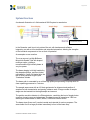
System Overview
A schematic illustration of a 2-dimensional SAXS system is seen below:
http://www.physics.queensu.ca/~
saxs/SAXSoverview.html
In the Ganesha, each item is truly state-of-the-art, with hardware and software
integration, as well as full motorization and extended automation, allowing the strengths
of the individual components to live out their full potential.
As examples we can mention:
The x-ray source is a High Brilliance
Microfocus Sealed Tube with shaped
multilayer optics, yielding a
monochromatic high intensity beam at
very low power.
The beam shaping is initially handled by
the shaped multilayer, and then further
collimated by 3 sets of 4-bladed slits, the
last of which contains single crystal
“Scatterless” blades.
The beam path is evacuated by an oil-free high speed pump allowing full pump-down to
clean operating pressures in 4 minutes.
The sample area comes with an XY-theta goniometer for alignment and position of
samples for both transmission and grazing incidence work. A large number of sample
stages can be inserted into the large sample environment
The position sensitive detector is a Pilatus detector, combining the best of single photon
counting, dynamic range and robustness. The detector can be moved over 1300 mm
allowing for measurement in WAXS, MAXS, SAXS and Extreme-SAXS.
The beam stops (there are 3) can be inserted and retracted for various purposes. The
same holds true for a large pin-diode immediately in front of the beam stop.
User Manual: UM-300-R1.1 dated 130112-01
Page 7 of 64
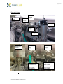
Getting Oriented on the System
Source, Optic, and Collimation
Optic
Collimation
Source
User Manual: UM-300-R1.1 dated 130112-01
Page 8 of 64
Sample Area
X-Ray
Lamp
Vacuum
Chamber
Sample Door
User Manual: UM-300-R1.1 dated 130112-01
Sample
Camera
and
Lens
Page 9 of 64
Sample Goniometer
Y-Z-Theta
Guard
Aperture
Z-stage
ZSAM
Y-stage
YSAM
Sample Viewer
mirror
(with hole for
X-ray beam)
ThetaStage
THSAM
User Manual: UM-300-R1.1 dated 130112-01
Beam
Entrance
Page 10 of 64
Detector Chamber, Motion, Beam Stop and Pin-diode
Detector
Chamber
Insertable
Round
Beamstop
Y-Motion
DETY
Z-Motion
DETZ
Insertable
Large
Pin-Diode
X-Motion
DETX
Insertable
Beamstop
User Manual: UM-300-R1.1 dated 130112-01
Page 11 of 64
Ports and Valves
Sample Area
Ports
Detector
Motion
Flange
Detector
Chamber
Flange
Evacuation
Valve
Vacuum
Gauge
Venting
Valve
Sample Area
Flanges
Detector
Motion
Flange
Image shown is for
Air-Cooled detector.
Uppor connectors will
differ for watercooled detector
User Manual: UM-300-R1.1 dated 130112-01
Detector
Chamber
Flange
Image Shown is for
Air-Cooled detector.
Water-cooled
detector will only
have one upper
electroni cable
Page 12 of 64
Electronics
Motor Drive and Controller
X-ray Generator and Controller
Instrument Control Computer
Detector Control Computer
Pin-diode meter (top) and
Voltage Analyser
User Manual: UM-300-R1.1 dated 130112-01
Vacuum Meter
Page 13 of 64
Vacuum Pumps (2 options)
h-Volume Dry-
Coolers (Source, Detector and Pump)
Detector and Source Cooler
Dry Pump Cooler
User Manual: UM-300-R1.1 dated 130112-01
Page 14 of 64
Sample holders and stages (not all may be available for your system):
8 mm between holes
Versatile Ambient Plate
ween
User Manual: UM-300-R1.1 dated 130112-01
Page 15 of 64
Linkam Heater Stage
Linkam Shear Stage
tal/Humidity Cell
er Segment
Linkam DSC
Linkam Tensile Stage
User Manual: UM-300-R1.1 dated 130112-01
Page 16 of 64
Getting Oriented on the Computer Desktop
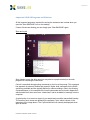
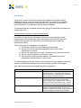
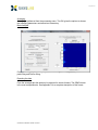
Startup Screen
The Instrument controlling computer (ICC) is a
linux computer running Ubuntu 12.04 LTS.
The login prompt will look like the image on the
right.
The account is
saxslab
And the password is
saxslab12
There are a number of looks that one may choose. The one we use is “gnome-classic
without features”
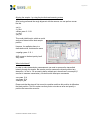
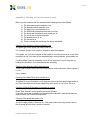
The 4 desktops and the 2 screens
Most instruments will have 2 side-by-side screens, where one screen will normally be
used for interacting with the programs and the others for monitoring. In this example we
have the control program “spec” in the leftmost window and the sample viewer in the
rightmost screen
In addition to these screens there are actually
4 individual desktops which can be accessed
by clicking on the icon in the lower right
corner of the left screen.
1
Such 4 screens are useful when one has many windows open.
User Manual: UM-300-R1.1 dated 130112-01
2
3
Desktops
4
Page 17 of 64
Minimizing windows
Windows can be closed, minimized or maximized by
clicking on the small icons in the upper left corner of
the window. The cross is closing, the “V” is minimizing
and the “upside-down V” is maximizing. When
minimized the windows can be found in the bar on the
bottom of the leftmost screen
General Organization Suggestions
Generally it is a good idea to keep similar tasks running in the same desktop.
Per default
 Desktop 1 is used for interactive instrument control and monitoring
 Desktop 4 is used for windows where various background processes are
running and reporting. These may be useful in case of trouble, but would
otherwise not be needed
 Desktop 2 and 3 could be used for data analysis and web-access.
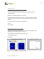
Starting up the SAXSLAB programs
On the desktop you will find an icon called “Start SAXSLAB”.
Right click this..and choose “open”. This action will first splash up a SAXSLAB banner
and then open up a whole array of programs and windows needed to run the SAXS
system. While this is happening the user should let the computer be.
When the banner
disappears, the user
can take control of
the computer again.
User Manual: UM-300-R1.1 dated 130112-01
Page 18 of 64
Important SAXSLAB Programs and Windows
All the important programs, required for running the instrument are invoked when you
open the “Start SAXSLAB” Icon on the desktop.
If some of these are missing you can simply open “Start SAXSLAB” again.
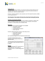
Spec and c-plot
Spec (shown here in the white terminal- may also be a purple terminal) is the main
program for controlling the instrument.
Control is exercised through writing commands on the line at the prompt. This command
line approach is extremely flexible and powerful. Higher level commands for the SAXS
system are available and are typically defined in macros residing in files in the directory
/usr/local/lib/spec.d. An incomplete list of useful commands can be found in Appendix 5,
which should at all times serve as a “cheat sheet” and be available in hardcopy near the
computer.
A typical action is to scan over a part of you sample and record the transmitted intensity.
The results of such a scan are plotted by the program C-plot, which is shown in the
upper part of the image above. The C-plot window will not normally be displayed when
Spec is started.
User Manual: UM-300-R1.1 dated 130112-01
Page 19 of 64
Sample Viewer (RayCam)
A completely standard and very useful feature of the
Ganesha SAXS system is the Sample Viewer which
has an on-axis view to the sample.
The combination of camera, lens and curved optic
(with a hole in it to let the x-ray through), actually
provide a microscope view of the sample that is
streamed to a small dedicated viewer.
The RayCam viewer is a new
internal development and has only
been with users since November
2012. Please report problems and
bugs so that we may address
them.
The viewer allows one to position a while a cross, which can then be used as a
reference for the beam position when aligning samples.
When you have defined the cross you may lock the position, so that it cannot be moved
(unless it is unlocked again). Several crosses can be defined, but only one shown at a
time.
One can calibrate the viewer so that the scale is actually represent real sizes.
Also one may use the viewer to zoom. It zooms in around the cross.
For documentation purposes one may also use the viewer to take a snapshot or even to
record the video stream.
Note: Due to curvature of the mirror straight lines may look curved. This is
User Manual: UM-300-R1.1 dated 130112-01
Page 20 of 64
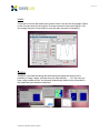
PyMCA
If one wants to look at the results from previous scans, one can use the program PyMca,
to look for scans saved in the log-files. All scans are saved in the current log-file. (You
can change the name of the log-file by using the spec command “newsample”)
SAXSGUI
SAXSGUI is the data-monitoring and data-reduction program that gives you the
possibility to image, reduce, plot and save your data manually…….or in the case you
have a large number of files…do the same automatically (based on the information in
the header and your reduction selections)
User Manual: UM-300-R1.1 dated 130112-01
Page 21 of 64
The various Servers:
Various servers are required to run in the background in order for everything to work
correctly:
Camserver – this server runs on the detector computer and talks directly to the
Detector. Should not be needed by the operator
Tvx- this server runs on the detector computer and can provide low-level
communication to Camserver if needed. Should not be needed by the operator.
Sl_server – this server runs on the detector computer and handles all of the
processing of the data in a measurement producing cumulative files and making
sure correct headers are included in the files. As of January 2013 this server also
does advanced noise-reduction.
Modbus_server – This server runs on the instrument control computer and
handles communication from spec to the Xenocs source generator…controlling
for example the opening and closing of the shutter and the High voltage and
current settings.
These various servers are usually reporting in Desktop 4
If any programs are missing you can get them back by invoking the “Start SAXLAB”
icon.
User Manual: UM-300-R1.1 dated 130112-01
Page 22 of 64
Data Output
Image data is saved in tiff format and should be readable by most data-handling
packages. However, since the header (see Appendix 1 for details on the header) is
stuffed with information about the measurement, full utilization of this information
requires SAXSGUI, or a dedicated customer header-interpreter
The measurements are numbered consecutively with pre-fix and suffixes indicating the
actually type of tile.
A measurement is actually a string of measurements
Per default, we have chosen that instead of making one long exposure for each
measurement, we will make many short measurements and then add these short
measurements together. We save both the summed image and the complete
measurement history.
There are a couple of advantages to this approach:
1) The dynamic range of the measurement becomes higher
2) We can observe the experiment progression each time the short
measurement is finished
3) We can use a time-slice of the data, if at some point the measurement fails
4) We can track the scattering as a function of time
5) We can perform advanced noise reduction, by comparing the short
measurement with each other in various ways.
For practical purposes we have chosen a time interval for the short measurements of 15
seconds. A 3600 second measurement therefore actually consists of 240 images.
As a result of the measurement the following files are generated:
Filename
/disk2/data/latest/latest_nnnnn_craw.tiff
/disk2/data/images/im_nnnnn_craw.tiff
/disk2/data/frames/frames_nnnnn_craw.zip
User Manual: UM-300-R1.1 dated 130112-01
Description
A tiff-file that is all the time updated to include the
latest taken data…i.e. this file is the “real-time”
sum of all the short measurements. This file has
the full header information inserted.
A tiff-file that is created at the end of the
measurement and is the sum of all the data
taken during the short measurements. It should
therefore be equal to the latest_nnnnn_craw.tiff.
This file has the full header information inserted.
A zip-file containing the short measurements as
well as a file with the Metadata. This file is not
readable by SAXSGUI..but may be processed for
cosmic background reduction from SAXSGUI.
Page 23 of 64
A Measurement
Initial Preparation
In the following we will assume that you (the user) will be running the system on your
own, but that the instrument responsible has made sure the instrument is prepared for
you…i.e. that the instrument is turned on, aligned, calibrated and basically ready to go.
However before commencing you will need to think a little about the experiment, prepare
the sample, check the instrument and mount the sample in the system.
Planning your measurement what are you looking for?
Before getting access to the instrument you should think about your measurement.
1) What q-range are you interested in?
2) How strongly does your sample scatter?
3) What are you looking for?
a. Peak Positions and peak-width?
b. Particle sizes?
c. Data that can be accurately modeled over a large q-range.
The answers to the above questions will determine how you run your experiment and for
how long you will run it.
Appendix 2 has a table of the available standard configurations for this system. It shows
aperture sizes, detector distances, q-range and intensities. In planning your
measurement understanding this table is crucial.
The first thing to realize is that in the routine running of the instrument you have a
unique chance to trade off resolution for intensity. The intensity available in the WAXS
configuration (configuration 1) is a factor of 4-5 higher than in the MAXS-configuration
and again a factor 4-5 higher than in the SAXS-configuration, and once again a factor 45 more than in the extreme SAXS regime. Flux is one of the most expensive things in an
x-ray instrument, so think about the resolutions (and the q-range) you need and run your
measurement accordingly.
In general, it is also our impression that users who are looking for Peak Positions and
Particle sizes spend much too much time measuring to get the low-intensity portions of
the curve to look nice. Think about what you are looking for, measure it to the accuracy
that you need and move on.
User Manual: UM-300-R1.1 dated 130112-01
Page 24 of 64
Checking the instrument performance
In order to use the system you need to make sure:
1) The instrument control computer is on
2) The detector control computer is on
3) The Motor Drive and controller is on
4) The SAXSLAB software environment is running
5) The pump and the pump-cooler are on
6) The x-rays are on and at full power
7) The pressurized air is on
8) The camera is on
9) That the remote disk containing the data is accessible.
If any of these are not satisfactory, you can contact the instrument responsible or try to
fix it yourself as outlined in Appendix 3.
If the system is not running at all you should contact the instrument responsible or try to
start it yourself as outlined in Appendix 4
Preparing and mounting the sample
Samples need to be prepared for measurement in vacuum. Depending on the samples
this may mean inserting them in disposable capillaries, putting them in sandwich cells,
inserting them in refillable capillaries or doing nothing at all. Please see Appendix 4 for
some inspiration.
Sample Alignment
Establishing a vacuum
When samples are mounted and everything is ready to go, the system should be
evacuated. This can be done with the spec command:
>evacuate_system
It will take roughly 4 minutes to reach the operating pressure of 2E-1 mbar. It is possible
to measure data long before this level has been reached, but the background scattering
from residual air will be too high for weakly scattering samples.
The vacuum will continue to improve over the evacuation time, but this will not affect the
measurements.
If 2E-1 cannot be reached please try to look for unattached hoses or other leaks or a
lack of pressurized air (which means the evacuation valve can not be opened)
Alternatively have the instrument responsible take a look.
User Manual: UM-300-R1.1 dated 130112-01
Page 25 of 64
Telling spec what sample holder is mounted
In order to make sure that the calibration holds for different sample holders it is
important that spec “knows” which stage is mounted.
The spec command:
>change_sample_stage
will give you a list of stages to choose from. Choose the correct one and proceed.
Note: There may be sample stages that have not been calibrated)
Goniometer Motions
The standard motors (and motions) in the sample goniometer are:



zsam--- Vertical motion (Z-axis) – A total travel of ~80 mm is available
ysam--- Horizontal motion (Y-axis) – A total travel of ~80 mm is available
thsam--- Rotation around the vertical Axis (thetat-motion) +-180 mdegrees.
The position of these motors (and all the others) can be seen by the spec-command:
>wu
The motors can be moved with the commands (examples):
>mv zsam 10
>umv ysam 40
>mvr zsam -5
>umvr thsam 1
The place where the beam hits the sample can be scanned by the command
>ascan zsam 30 45 15 1 (which scans zsam from pos 30 to 45 in 15 intervals counting
1 second per interval)
>dscan ysam -3 3 12 1
(which scans ysam relatively from relative pos -3 to relative
position 3 in 12 intervals counting 1 second per interval)
However do remember to insert the pin-diode, and open the x-ray shutter, so the overall
measurement will have the following command flow:
User Manual: UM-300-R1.1 dated 130112-01
Page 26 of 64
>pd_in
>o_shut
>dscan ysam -3 3 12 1
>c_shut
>pd_out
A scan of a hole in a sample in a block
could look like this.
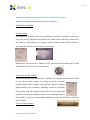
Aligning the sample –by using the on-axis camera
The on-axis camera helps to obtain a rough idea
of where the sample is.
The cross indicates where the beam is. And one
can then use a transmission measurement
combined with a scan (as immediately above) to
do a fine alignment.
User Manual: UM-300-R1.1 dated 130112-01
Page 27 of 64
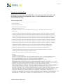
Aligning the sample – by using the pin-diode and scanning motors
After having performed the rough alignment with the camera, one can perform a scan
like this.
>pd_in
>o_shut
>dscan ysam -3 3 12 1
>c_shut
>pd_out
This could yield this plot, which we could
analyze to determine the best sample
position.
However, for capillaries there is a
dedicated routine, that does the same
>capalign ysam -3 12 1
AND moves to the best spot by itself.
Very useful.
Where’s the blank?
In order to make transmission measurements, we need to measure the transmitted
intensity through the sample. But we also need to measure the intensity without any
absorption, i.e. the Io.. So we need to define a blank spot, where there is no sample (if
we want to measure transmission). We do this with these spec commands
>mv ysam 12.4
>mv zsam 35.4
>blankpos_def
Please note that the stage is first moved to a position and then this position is defined as
the blank position. This is to make sure that you do not make an error and specify a
position that cannot be moved to.
User Manual: UM-300-R1.1 dated 130112-01
Page 28 of 64
Pre-measurement Actions
Choosing a q-range /configuration
Based on the table of the various configurations in Appendix 2, one can decide which
combination of resolution, q-range and intensity is desired. Once this has been decided,
one can go to this configuration using the spec command:
>conf_ugo N…..where N is the number of the configuration (forexample conf_ugo 1)
Letting the computer adjust the beam stop position
It has been our experience that the most sensitive alignment is the location of the
detector with respect to the beam, which ultimately means the location of the beam stop
with respect to the beam. In order to correct for this, the system has a small routine
which can be executed on its own.
So if you wish, you may run the spec command:
>mv_beam2bstop
to center the beamstop on the beam.
Note: This routine relies on the beamstop being centered on a reference position on the
detector. If for some reason it is not centered on here (someone bumped or similar) then
one will have to redefine either motor positions or this reference positioned as described
in the “Expert Users FAQ”
Measuring Io and the sample transmission
If a blank position has been defined, one can issue the command:
>transmission_measure
to measure the Izero as well as the transmission, using the pin-diode.
The Izero is stored in the spec variable I0 and the transmission is stored in the variable
SAMPLE_TRANS.
User Manual: UM-300-R1.1 dated 130112-01
Page 29 of 64
Describing the measurement
For entering into the header, as well as the super log file (master.dat) one may define
the value of the spec variable SAMPLE_DESCRIPTION like this:
>SAMPLE_DESCRIPTION=”This is my sample in configuration 3 measured for 300
seconds”
This string is then saved to the file header and displayed in SAXSGUI when the file is
loaded.
Additional Reduction Parameters
In addition to these measured parameters one can also enter the following parameter
>SAMPLE_THICKNESS=0.1
#where thickness is given in cm
Beam Stop Mask
To facilitate quick data-reduction one can also specify a beamstop mask that will be
applied to the data when reduced in SAXSGUI. A beamstop mask particular to each
configuration has been defined. To invoke this feature one can write
>use_bsmask
NOTE: All these reduction parameters SAMPLE_DESCRIPTION, SAMÅLE
THICKNESS and use_bsmask are reset after a successful measurement.
Telling SPEC that it is for real
The command
>saxson
is a necessary command to tell spec that this measurement is for real and that it needs
to establish connection to the detector computer. It can be entered anytime and is
assumed “on” until a saxsdiscconnect command is given.
Pre-measurement routine
So the preparation of a measurement could look like:
>evacuate_system
>do_sleep (250)
User Manual: UM-300-R1.1 dated 130112-01
Page 30 of 64
>conf_ugo 2
>saxson
>mv_beam2bstop
>mv ysam ysamblank
>mv zsam zsamblank
>blankpos_def
>mv ysam ysam_roughpos
>mv zsam zsam_roughpos
>capalign ysam 2 40 1
>transmission_measure
>SAMPLE_DESCRIPTION=”my sample”
> use_bsmask
> SAMPLE_THICKNESS=0.1
User Manual: UM-300-R1.1 dated 130112-01
Page 31 of 64
The Measurement
The Measurement command and on-screen feedback
Given all the preparation from before we now just need to issue the command
>saxsmeasure time
Where time is the desired exposure time in seconds.
Once the measurement has started, a number of messages are output to the spec
window. One should just look at the output screen to make sure that a file is actually
recording.
If it is not recording it is likely that one has forgotten the
>saxson
spec-command.
Monitoring the measurement from SAXSGUI
SAXSGUI has recently been upgraded to allow it to monitor the development of the
data-gathering both in a 2D image and in a 1D plot.
This functionality can be obtained by accessing the menu:
>File >Open Latest (cont)
In SAXSGUI
User Manual: UM-300-R1.1 dated 130112-01
Page 32 of 64
Monitoring the measurement remotely by Teamviewer
All systems come with Teamviewer installed. Teamviewer is a state of the art desktop
sharing software, with free usage for non-commercial use.
With Teamviewer, the operator may monitor the system from a remote location.
Naturally such access is dependent on the internet access policy of the organization
User Manual: UM-300-R1.1 dated 130112-01
Page 33 of 64
Interactive Data Reduction
SAXSGUI is the main data-reduction tool available with the system. It has its own
manual and even its own basic website (www.saxsgui.com).
The source-code can be found at
http://www.saxsgui.com/latest_saxsgui_saxslab.zip
The latest executables can be found at
http://www.saxsgui.com/latest_saxsgui_SLlinux32.zip (linux 32-bit)
and
http://www.saxsgui.com/latest_saxsgui_SLwin32_prg.exe (windows 32-bit))
If one already has the appropriate Matlab Runtime Library one can choose to download
instead
http://www.saxsgui.com/latest_saxsgui_SLwin32.exe
which is just the program.
The latest manual (often not completely current) can be found at
http://www.saxsgui.com/latest_manual.pdf
or
http://www.saxsgui.com/latest_manual.doc
User Manual: UM-300-R1.1 dated 130112-01
Page 34 of 64
Viewing the data
SAXSGUI was originally created for very interactive viewing of data collected on less
automated instrumentation. It therefore features a long list of interactive methods to
visualize, alter, center and calibrate the data.
However, it has been adapted to make extensive use of the header information available
in the Ganesha data file.
As a result when a file is opened, both the image, the polar plot and the radial average
will be displayed. Each window has a range of tools and menus for displaying the data.
Interactive Centering and Calibrating
Due to the program history there is a long list of interactive methods to visualize, alter,
center and calibrate the data, which will normally not be required, as the relevant
information is usually already in the metadata header.
Reductions
Some reductions are presently available in the metadata
 transmission correction
 intensity correction
 sample thickness correction
 beam stop mask
However relational reductions (relating to other files) such as
 empty holder reduction
 darkcurrent reduction
 zinger reduction
are not presently supported in the Ganesha meta-data format.
To reduce the data further one may
therefore use the Reduction Panel in the
Reduction Menu.
This panel will be filled with parameters from
the metadata header and relational files can
be added.
Masking
In the reduction panel “File” menu there is a
Create Mask item. This will open up
MaskMaker which is a mask-building tool for
SAXSGUI.
User Manual: UM-300-R1.1 dated 130112-01
Page 35 of 64
Averaging
Averaging is performed from the processing menu. The GUI gives the options to choose
the averaging parameters and reductions interactivey.
Basic Analysis
From the averaged plot one may inspect the data and perform simple analysis such as
peak-fitting and Guinier fitting.
Exporting the data
From the averaged plot the data may be exported in various formats. The GRAD format
is the most comprehensive. See Appendix 6 for a complete description of this format.
User Manual: UM-300-R1.1 dated 130112-01
Page 36 of 64
User Manual: UM-300-R1.1 dated 130112-01
Page 37 of 64
Automated Processing(AP) (based on the metadata header)
SAXSGUI has been expanded to automate a lot of the tedious tasks associated with
data reductions, using the information in the metadata-header.
Quick Experiment Overview
If one uses the “Next” and “Previous” buttons in the panel, one can quickly investigate a
series of measurements.
The radial average plot of each new image is added to the plot.
Note. If the number of datasets plotted become too large simply close the window.
Exporting the AP data
When many files are generated, the interactive reduction becomes tedious. However,
using the metadata information, it is possible to automatically process the files and save
 2D images
 1D plots
 Data in SAXSLAB GRAD format (see Appendix 7 for examples)
This can be done by going to Processing->Autoprocess-AP with Metadata. Then you will
be prompted for which files to process and which directory to save the processed data
to.
Tips for Exporting the AP-data
The automated processing uses the sizes of the windows to generate the images. If you
find that the plots in the automated images do not look nice, try making the size of the
window larger.
Known Limitations in AP on the Ganesha
SAXSGUI (as in any other software package) in always in development, with a
timeframe determined by priority and difficulty.
User Manual: UM-300-R1.1 dated 130112-01
Page 38 of 64
Many Measurements
In the previous sections, we showed how to prepare and measure a single sample in a
single measurement.
Of course normally one would want to investigate the sample for a broader range of qvalues than accessible with a single measurement or measure several samples. Both
examples are explored below
Examples of many measurements
Changing configurations
The command for changing configurations was
conf_ugo configuration_number
which becomes useful, for example, with many measurements of a capillary over many
configurations:
evacuate_system #Evacuate the system
do_sleep (250)
#Waits for the evacuation
conf_ugo 2
#Go to configuration 2
saxson
#Make sure spec knows we want to communicate
mv_beam2bstop
# Adjust the detector
mv ysam ysamblank # Move to the Y-position of the blank sample position
mv zsam zsamblank #Move to the Y-position of the blank sample position
blankpos_def
#Define this position as the blank
mv ysam ysam_roughpos
#Move to the sample Y position (nominal)
mv zsam zsam_roughpos
#Move to the sample Zposition (nominal)
catalign ysam 2 40 1
#Align the capillary
transmission_measure
# Measure the sample transmission and Izero
SAMPLE_DESCRIPTION=”my sample in conf 2”
use_bsmask
#Use a beamstop mask for processing
SAMPLE_THICKNESS=0.1 #Use a sample thickness in cm for processing”
saxsmeasure time
#Measure for an amount of time
#Now for new configuration
conf_ugo 2
# Go to configuration 2
mv_beam2bstop
# Adjust the detector
transmission_measure
#Measure Sample transmission and Izero
SAMPLE_DESCRIPTION=”my sample in conf 2”
use_bsmask
#Use a beamstop mask for processing
SAMPLE_THICKNESS=0.1 #Use a sample thickness in cm for processing”
saxsmeasure time
#Measure for an amount of time
User Manual: UM-300-R1.1 dated 130112-01
Page 39 of 64
Changing Samples
Another example is moving to a different location:
evacuate_system #Evacuate the system
do_sleep (250)
#Waits for the evacuation
conf_ugo 2
#Go to configuration 2
saxson
#Make sure spec knows we want to communicat
mv_beam2bstop
# Adjust the detector
mv ysam ysamblank # Move to the Y-position of the blank sample position
mv zsam zsamblank #Move to the Y-position of the blank sample position
blankpos_def
#Define this position as the blank
mv ysam ysam_roughpos1 #Move to the sample Y position (nominal)
mv zsam zsam_roughpos1 #Move to the sample Zposition (nominal)
catalign ysam 2 40 1
#Align the capillary
transmission_measure
# Measure the sample transmission and Izero
SAMPLE_DESCRIPTION=”my sample #1 in conf 2”
use_bsmask
#Use a beamstop mask for processing
SAMPLE_THICKNESS=0.1 #Use a sample thicknes in cm for processing”
saxsmeasure time
#Measure for an amount of time
#Now for new sample
ysam ysam_roughpos2
#Move to the sample Y position (nominal)
mv zsam zsam_roughpos2 #Move to the sample Zposition (nominal)
catalign ysam 2 40 1
#Align the capillary
transmission_measure
# Measure the sample transmission and Izero
SAMPLE_DESCRIPTION=”my sample #2 in conf 2”
use_bsmask
#Use a beamstop mask for processing
SAMPLE_THICKNESS=0.1 #Use a sample thicknes in cm for processing”
saxsmeasure time
#Measure for an amount of time
User Manual: UM-300-R1.1 dated 130112-01
Page 40 of 64
Constructing advanced sample descriptions
From the 2 examples above you can see there is a lot of repetition involved in these
cases. Yet, generally, you want the sample description to be quite specific about the
measurement, so here is a way to construct a very specific header.
Let’s say
myconf=2
conf_ugo myconf
saxson
#Make sure spec knows we want to communicat
mv_beam2bstop
# Adjust the detector
mv ysam ysamblank # Move to the Y-position of the blank sample position
mv zsam zsamblank #Move to the Y-position of the blank sample position
blankpos_def
#Define this position as the blank
mv ysam ysam_roughpos1 #Move to the sample Y position (nominal)
mv zsam zsam_roughpos1 #Move to the sample Zposition (nominal)
catalign ysam 2 40 1
#Align the capillary
transmission_measure
# Measure the sample transmission and Izero
strtmp=sprintf(“Blah conf %i , IO=%i, T=%f” (myconf, Io,SAMPLE_TRANS))
SAMPLE_DESCRIPTION=strtmp
saxsmeasure 300
The sprintf command prints the values of myconf, izero and SAMPLE_TRANS to the
Sample Description String.
Sprintf uses the same syntax for formatted output as the common computing commands
sprint and fprintf.
Constructing a macro for multiple actions (with gedit)
Rather than writing all of these commands on the spec command line, they can be put in
a txt-file. There is a decent text editor available (gedit) which can be used to write the
series of command
Executing a macro from Spec
With the file is saved it is possible to call this “macro-function” by the following spec
command
qdo directory/filename
User Manual: UM-300-R1.1 dated 130112-01
Page 41 of 64
An Experiment
The nature of an experiment
The above examples have all been examples of simple measurements, i.e.
1) Measure a sample for a certain amount of time in one configuration
2) Measure a sample in a number of different configurations
3) Measure many samples in one or more configurations
But often there is a need to do more complicated measurements, where typical
characteristics of the sample are altered. For example, performing measurements at
different temperatures.
In these more complicated scenarios, we speak of experiments. Due to their complexity,
the experiments yield themselves well to inserting the command sequences into macros
Free-form or loops in SPEC
An experiment can of course be written into a macro as a series of individual
measurements (the freeform – commands shown are not actual spec command)
Prepare experiment
Set temperature to 10 degrees
Describe Sample
Measure
Set temperature to 12 degrees
Describe Sample
Measure
But one can also use the loop structures available in spec
Prepare experiment
For (icnt=1;icnt<5;icnt++) {
Mytemp =( icnt-1)*2+10
set temperature to Mytemp
Describe Sample
Measure
}
This loop will measure 5 times, starting at 10 degrees and finishing at 18.
In such cases, it is very useful to construct the advanced sample descriptions as
discussed above as for example:
SAMPLE_DESCRIPTION=sprintf(“My Great Sample Temp=%d”;Mytemp)
User Manual: UM-300-R1.1 dated 130112-01
Page 42 of 64
Varying position
To vary the position or angle of the sample one can use the commands
mv, umv, mvr, umvr
as discussed earlier in this manual.
The sample motors that can be manipulated are
ysam, zsam, and thsam
So a position scan could look as follows
for (icnt=0;icnt<10; icnt++) {
ysamstart=42
ysamstep=1
ysampos=ysamstart+icnt*ysamstep
mv ysam ysampos
SAMPLE_DESCRIPTION=sprint(“Mysample ysam=%d”,A[ysam])
use_bsmask
saxsmeaure 600
}
And of course one could make a 2D scan by enclosing the above loop within another
loop
for (icnt1=0;icnt1<10; icnt1++) {
zsamstart=10
zsamstep=1
zsampos=zsamstart+icnt1*zsamstep
mv zsam zsampos
for (icnt2=0;icnt2<10; icnt2++) {
ysamstart=42
ysamstep=1
ysampos=ysamstart+icnt2*ysamstep
mv ysam ysampos
tmp= sprint(“Mysample xsam=%d, ysam=%d”, A(ysam), A(zsam))
SAMPLE_DESCRIPTION=tmp
use_bsmask
saxsmeaure 600
}
}
User Manual: UM-300-R1.1 dated 130112-01
Page 43 of 64
Varying Temperature with the Julabo Circulating Heater/Chiller
Useful Commands for the Julabo
Julabo Thermostated Bath
julabo_start
Switches ON the Julabo Unit
julabo_end
Switches OFF the Julabo Unit
julabo_stabilise s_p stabilization_time maxtime
Sets setpoint to s_p and logs temperature until the temperature is
reached. After the temperature is reached it stabilizes for the
given time. If reaching the temperature takes more than maxtime
then the command is stopped
_julabo_get_temperature()
Returnt the temperature of Julabo stage
julabo_get_temperature
Prints out the current temperature to the screen
An example macro
julabo_start
for (icnt=0;icnt<10; icnt++) {
mytempstart=42
mytemstep=0.5
mytemp=mytempstart+icnt*ysamstep
julabo_stabilise mytemp 300
tmp= sprint(“Mysample temp=%d”,_julabo_get_temperature())
SAMPLE_DESCRIPTION=tmp
use_bsmask
saxsmeaure 600
}
julabo_end
User Manual: UM-300-R1.1 dated 130112-01
Page 44 of 64
Varying Temperature with the Linkam Heater stage
Useful Commands for the Linkam Heater Stage
Linkam Thermal Stage Commands
linkam_start
Switches ON communication with Linkam Controller (overhead cost =
4 seconds)
linkam_end
Switches OFF communication with Linkam Controller
linkam_pump_auto
Start the Linkam pump in auto mode. Manual mode can also be set
Linkam_pump_manual, and then Linkam_set_pumpspeed. But this is
not recommended
linkam_stabilise s_p maxtime
Sets setpoint to s_p and logs temperature until the temperature is
reached. Unless maxtime is exceeded.
_linkam_get_temperature()
Returns current temperature of Linkam stage
linkam_get_temperature
Get current temperature of Linkam stage
linkam_get_rate
Get current ramp rate for Linkam stage
linkam_get_setpoint
Get current setpoint for Linkam stage
linkam_set_rate rate
Sets the temperature ramp rate to rate degrees per minute
linkam_set_setpoint temp
Sets the temperature to temp degrees
linkam_set_pumpseed nn
Sets the pumpspeed to nn%
linkam_watch maxtime
Logs the temperature for maxtime
linkam_cool
Cools the Linkam stage as fast as possible
An example macro
linkam_start
linkam_pump_auto
linkam_set_rate 10
for (icnt=0;icnt>10; icnt++) {
mytempstart=80
mytemstep=5
mytemp=mytempstart+icnt*ysamstep
linkam_stabilise mytemp 180 900
tmp= sprint(“Mysample temp=%d”,_linkam_get_temperature())
SAMPLE_DESCRIPTION=tmp
use_bsmask
saxsmeaure 600
}
linkam_end
User Manual: UM-300-R1.1 dated 130112-01
Page 45 of 64
Appendix 1: The SAXSLAB metadata-header
#
#
#
#
#
#
#
#
#
#
#
#
#
#
#
#
#
#
#
#
#
#
#
#
#
#
#
#
#
#
#
#
#
#
#
#
#
#
#
#
#
#
#
#
<SAXSLAB METADATA START>
datatype: tiff
detectortype: PILATUS 300K
start_timestamp:
end_timestamp:
save_timestamp:
realtime:
livetime:
1800.00
pixelsize: 0.172 0.172
beamcenter_nominal:
338.50
beamcenter_actual:
338.47
<DATA METADATA START>
data_mean:
data_min:
data_max:
data_rms:
data_p10:
data_p90:
<DATA METADATA END>
<CALIBRATION METADATA START>
calibrationtype: geom
kcal:
pixelcal:
koffset:
wavelength: 1.5408
detector_dist: 1056.2000
<CALIBRATION METADATA END>
<CONFIGURATION METADATA START>
saxsconf_r1:
saxsconf_r2:
saxsconf_r3:
saxsconf_l1:
saxsconf_l2:
saxsconf_l3:
saxsconf_l4:
saxsconf_wavelength: 1.5408
saxsconf_dwavelength: 0.01
saxsconf_Izero: 211338
saxsconf_det_offx: 0
saxsconf_det_offy: 0
saxsconf_det_rotx: 0
saxsconf_det_roty: 0
saxsconf_det_pixsizez: 0.172
saxsconf_det_pixsizey: 0.172
User Manual: UM-300-R1.1 dated 130112-01
201.50
201.42
Page 46 of 64
#
#
#
#
#
#
#
#
#
#
#
#
#
#
#
#
#
#
#
#
#
#
#
#
#
#
#
#
#
#
#
#
#
#
#
#
#
#
#
#
#
#
#
#
#
#
#
saxsconf_det_resx_0:
saxsconf_det_resy_0:
saxsconf_abs_int_fact:
<CONFIGURATION METADATA END>
<SAMPLE METADATA START>
sample_transfact:
0.00000
sample_thickness:
sample_xpos:
sample_ypos:
sample_angle1:
sample_angle2:
sample_angle3:
sample_temp:
sample_pressure:
sample_strain:
sample_stress:
sample_shear_rate:
sample_concentation:
<SAMPLE METADATA END>
<SPEC METADATA START>
hg1: 0.299975
hp1: 0.084741
vg1: 0.299975
vp1: -0.010509
hg2: 0.149987
hp2: 0.003747
vg2: 0.149987
vp2: 0.051181
hg3: 0.360010
hp3: 0.009861
vg3: 0.360010
vp3: 0.093097
ysam: 41.840000
zsam: 39.290000
thsam: 0.000000
detx: 950.000000
dety: -0.815313
detz: 0.890944
bstop: 42.120000
pd: 10.000000
<SPEC METADATA END>
<GENERATOR METADATA START>
source_type: MM002+
source_runningtime:
source_kV: 42 kV
source_ma: 0.95 mA
<GENERATOR METADATA END>
User Manual: UM-300-R1.1 dated 130112-01
Page 47 of 64
# <DEFAULT REDUCTION RECIPE
# xaxis:
# xaxisfull:
# yaxis:
# error_norm_fact: 1
# xaxisbintype: lin
# log: log
# reduction_type: s
# reduction_state:
# raw_filename:
# mask_filename:
# flatfield_filename:
# empty_filename:
# solvent_filename:
# darkcurrent_filename:
# readoutnoise_filename:
# zinger_removal: 0
# data_added_constant: 0
# data_multiplied_constant:
# <DEFAULT REDUCTION RECIPE
# <SLDS START>
# Img.Class:
# Img.MonitorMethod:
# Img.ImgType: 2D
# Img.Site: KU-LIF
# Img.Group:
# Img.Researcher:
# Img.Operator:
# Img.Administrator:
# Img.Description
# Meas.Description: PSPEO-a
MeasTime=1800.000000
# <SLDS END>
# <SAXSLAB METADATA END>
User Manual: UM-300-R1.1 dated 130112-01
START>
1
END>
Conf 3, Temp=110.000000,
Page 48 of 64
Appendix 2: Standard Configurations
Conf
Mne
Description
DETX
Ideal
beam
stop
NA
Aperture
size
(mm)
4-4-5
qmin
50
Sample
DetDist
NA
0
Open
1
WAXS
Open
Apertures
Wide Angle
2
MAXS
3
4
50
~180
2mm
0.05
2.5
20
Medium
350
480
2mm
0.012
0.67
6
SAXS
SAXS
950
1080
2mm
0.006
0.26
1.5
ESAXS
Extreme
SAXS
1400
1540
2mm
0.7-0.41.0
0.4-0.30.7
0.3-0.150.4
0.2-0.10.3
0.003
0.21
0.3
User Manual: UM-300-R1.1 dated 130112-01
qmax
Io
Mphs
80
Page 49 of 64
Appendix 3: Checking that the instrument is ready
Before you can measure with the instrument the following have to be fullfilled:
1)
2)
3)
4)
5)
6)
7)
8)
9)
The instrument control computer is on
The detector control computer is on
The Motor Drive and controller is on
The SAXSLAB software environment is running
The pump and the optional pump-cooler are on
The x-rays are on and at full power
The pressurized air is on
The camera is on
That the remote disk containing the data is accessible.
Checking if the instrument control computer is on:
The green light on the upper right hand corner is on.
If it is Orange, press it for a couple of seconds to start the computer.
If it is green, but you have no signal on the monitors, move the mouse a bit, to see if the
monitors liven up. If not then try the standard things: mouse-batteries, loose cables, etc.
If nothing helps, it may be necessary to turn off the Instrument Control Computer by
holding the on-button in for 8 seconds and then restarting
Checking if the detector control computer is on
There is here a button on the left side of the detector control computer, which is green if
it is on.
If not…press it.
Checking if the Motor Drive and controller is on
The Motor Drive and Controller is on if the green light on the front panel toggle button is
on. There should also be a clearly audible hum from the fan. If it is not on, turn it on.
Checking if SAXSLAB software environment is running
Press “Start Saxslab” to start opening the all the software.
If you later notice that something has not started this indicates a serious fault and you
should contact your instrument responsible.
Checking if the pump and cooler is on
You will be able to hear, if these are on. If the pump cooler for the dry pump is not on,
the dry pump will stop after a couple of minutes.
User Manual: UM-300-R1.1 dated 130112-01
Page 50 of 64
Checking if the x-rays are on and at full power
If X-rays are on, the orange lamp on top of the instrument will be lit.
If the generator is at full power the settings should be close to 50kV, 60mA (but slightly
below).
You can also inquire about these values by using the spec commands
>p genix_get_HT()
>p genix_get_current()
Checking if the pressurized air is on
Pressurized air is required for purging the detector (clean dry air) and providing power to
open the ventilation and evacuation valves.
You should hear a slight hissing from the pipes, if the air is on. You can also try to
operate the vent valve by using the spec commands:
>ventvalve_open
>ventvalve_close
and listening for the sound of air hissing as the valve changes state.
Checking to see if the camera is on
There will be 2 green lights on the camera underside. Power and Communication. Of
course the image should also be displayed in the sample viewer window.
Checking to see if the remote disk (/disk2) is mounted
Data is located on the detector computer disk, which is remotely mounted for access.
To check if the remote disk has mounted correctly, open a terminal on the linux desktop
and write
ls /disk2/data
This command should list the directories latest, images, frames and stats
If not please run the command
sudo mount –a
and test again. If it still fails contact the instrument responsible
User Manual: UM-300-R1.1 dated 130112-01
Page 51 of 64
Appendix 4: Sample Preparation for the Ganesha SAXS system
With heavy inspiration from Ronit Bitton, Ben Gurion University
Preparing the sample(s)
Powder samples
If the samples are powders, they can conveniently be mounted in a capillary or in between
two pieces of tape. Sometimes using the hole of a small washer (with tape on both side of
the washer is a good simple way to prepare a thicker powder sample. 3M Scotch tape is
fairly good but does have some weak low-q scattering.
Alternatively, one can use the “Sandwich Cells” provided for the Linkam stage, and fill
them as described for Viscous Liquid Samples
Non-viscous Liquids samples
Non-viscous liquids can be inserted into a capillary. The capillary should be sealed either
by wax, glue or flame-sealing, or by using one of the “reusable”
capillary holders where sealing is done with an O-ring.The capillary
should ideally be free of bubbles; containing as little air as possible
(the pressure from the residual air has been known to break some
capillaries). Please treat capillaries with care. Free-standing capillaries
are typically 3-4 € per piece and reusable capillaries are more than 500€ (up to 1000 € by
some vendors)
Viscous Liquids samples
User Manual: UM-300-R1.1 dated 130112-01
Page 52 of 64
Viscous liquids are difficult to get in and out of capillaries. As a consequence we use
holders where the viscous liquids are sandwiched between 2 thin sheets of either Mica or
Kapton (10 mm diameter). These are intended for use with the Linkam stage, but can be
mounted anywhere.
We prefer Mica windows, since scattering is very low and very uniform. However, since
absorption is high in Mica, the windows must be very thin, and thus unfortunately become
costly. ~4 € for 5-7 micron thick window.
SAXSLAB can supply the required Mica sheets.
User Manual: UM-300-R1.1 dated 130112-01
Page 53 of 64
Mounting the sample(s)
The systems would normally be supplied with this stage

A 2D ambient temperature stage, where 42 sample positions
are provided
And may then contain the following optional stages

A JSP multi-capillary holder for capillaries (both
refillable and non-refillable) with temperature control
(5-70C).

A special vacuum adapted Linkam thermal stage for thermal analysis, which
allows for mounting one flat solid sample, one capillary inserted into the thermal
block or one sandwich cell. Temperature range is -150C-300C
The maximum heating/cooling rate of 30 C/min.
User Manual: UM-300-R1.1 dated 130112-01
Page 54 of 64
Generic Stage:
Samples can be fixed to the generic stages by using tape, vacuum
grease, wax or holes in the sample holder that fit the pins on the
generic stage.
Capillaries should be mounted vertically.
The sample holder is inserted into the chamber by sliding it into
the gap in the sample stage
The writing on the side of the sample holder should be facing
the chamber door (you)
GISAXS in generic holder
Tape the sample in the middle of the sample holder sticking out on top
The sample holder is inserted into the chamber by sliding it into the gap in the sample
stage
Multi-capillary holder:
This holder fits 6 capillary metal cartridges. The cartridges should be
filled, capped and inserted all the way into the holder. A pin will ensure
that they are placed reproducibly.
User Manual: UM-300-R1.1 dated 130112-01
Page 55 of 64
Linkam thermal stage:
The stub below the thermal block should be fitted with a spring which forces the sample
or the sandwich holder up against the block. The springs supplied by Linkam have a
“lollipop” shape and there is 1 such “lollipops” provided
It should be possible to change samples without taking out the block
For samples in capillaries an alternative mounting approach is used, in that the capillary
can be inserted horizontally into a small (1.6 mm) hole in the block. 1 and 1.5 mm
capillaries should fit. With a little bit of care the capillary can be inserted from outside the
stage body.
Alternatively one can screw a small lid on the heater plate, and insert the capillary into this
lid.
User Manual: UM-300-R1.1 dated 130112-01
Page 56 of 64
Appendix 5: Ganesha SAXS installation- SPEC Quick Reference (12/06/20)
Most used Commands
vent_system, evacuate_system
Vent and evacuate the SAXS system
c_shut, o_shut
Close and Open the Shutter
conf_go, conf_ugo, what_conf
Go to a predefined configuration, update
mv, umv, mvr, umrv
Moves motors in different ways
wu
Shows motor positions
ascan, dscan, lup
Different types of motor scans
pd_in , pd_out
Move pin diode detector into the beam
SAMPLE_DESCRIPTION=”hello”
Sets a parameter that is written to master.dat and image header
saxsmeasure , killsaxsmeasure
Takes and image and saves it, kill the saxsmeasurement
completely
transmission_measure, blankpos_def
Measures the transmission of a sample, define blank position
qdo macro-file
Execute the commands in the macrofile (quiet do)
mv_beam2bstop
Centers the beam on the beamstop
Light_on, Light_off
Centers the beam on the beamstop
Standard SPEC Commands
>spec
to run spec-session from UNIX window
wa
list of all defined motors with its user and dial values
wu
list of all defined motors with its user values
wm
motor-name1 motor-name2 ...
where motors: user and dial values, soft limits of motors
mv
motor-name number
absolute move of a motor by number [mm] or [º]
mvr
motor-name number
relative move of a motor by number [mm] or [º]
umv motor-name number
updated absolute move of a motor by number [mm] or [º]
umvr motor-name number
updated relative move of a motor by number [mm] or [º]
ascan motor-name init_value final_value
nº_of_steps time_per_step
absolute scan – remember to open shutter before running this
dscan motor-name init_value final_value
nº_of_steps time_per_step
relative scan – remember to open shutter before running this
lup motor-name init_value final_value nº_of_steps
time_per_step
relative scan, which goes to the peak afterweards
counters
define your counters
setplot
define parameters of the plot on the screen
plotselect
define counters to be plotted
Ctrl-C
stop execution of a command
newsample
Allows to define parameters for new sample (filename, plot
window etc)
User Manual: UM-300-R1.1 dated 130112-01
Page 57 of 64
prdef macro-name
listing of commands in a known macro
lsdef *name*
list of known macros conatining string name
Beam stop and Pin-diode Related Commands
change_bstop_conf
Change the desired beam stop position/configuration
bstop_in
Move the beam stop into nominal position
bstop_out
Move the beam stop out of the detector area
pd_in
Move Pin-diode into beam
pd_out
Move Pin-diode out of beam
Configuration Related Commands
what_conf
Ask what configuration is most likely the present
conf_go conf#
Go to the configuration specified (using configuration variables)
conf_ugo conf#
Go to the configuration specified (using configuration variables) –
updating positions
conf_lineup conf#
Create lineup procedure for configuration specified
full_conf_lineup conf#
Create lineup procedure for configuration specified including
detector alignment
detpos_go conf# detpos_ugo conf#
Go to the detector position in the specified configuration
conf_save conf#
Save the present pinhole location to the pinhole configuration
variables
conf_save2disk
Saves the present pinhole configuration variables to a file that
can later be reloaded
conf_load_latest
Loads latest saved pinhole positions
conf_load_default_positions
Loads old default positions
Source and Detector-Related Commands
(remember “remote mode” for generator)
o_shut
Open X-ray Shutter
c_shut
Close X-ray Shutter
x_start
Starts X-ray generator and goes to standby mode
x_ramp
Ramps the X-ray generator and goes to full power
x_standby
Moves the X-ray generator to standby values
x_off
Turns the generator off
User Manual: UM-300-R1.1 dated 130112-01
Page 58 of 64
SAXS-Related Commands
saxson
Prepares SPEC for SAXS image measurements
saxsconnect
Connect and control Pilatus Camserver
saxsdisconnect
Releases control of the Pilatus Camserver
saxsoff
Releases SPEC from SAXS image measurements
saxsmeasure time
Measures for a total of time seconds saving an images each 15
seconds (FRAME_TIME=15). Filename is consecutive
saxsmeasure_free time
Measures for time seconds and saves the image. Filename is
consecutive number
saxsmeasure_temp time
Measures for time seconds and saves the image in a temporary
file called temp.tiff
saxsmeasure_cont time
Continuously measures images time seconds long and saves
the images in a temporary file called temp.tiff (which are
continuously overwritten)
saxsmeasure_freefile time filename
Measures for time seconds and saves the image in a file called
filename.tiff
SAMPLE_DESCRIPTION=sprintf(“bla”)
Gives the next saved file a brief description
blankpos_def
Defines a blank position (no sample)
Transmission_measure
Measure the relative transmission at this location (with respect
to the blank)
Vacuum Related Commands
evacuate_system
Evacuate the SAXS system
vent_system
Vent the SAXS system
Misc commands
Capalign motor half-range #intervals
User Manual: UM-300-R1.1 dated 130112-01
Performs an absorption scan of a capillary in a hole and move to
the capillary center
Page 59 of 64
Julabo Thermostated Bath
julabo_start
Switches ON communication with Julabo Controller (overhead
cost = 4 seconds)
julabo_end
Switches OFF communication with Julabo Controller
julabo_counter_on
Start using Julabo as a counter (to Julabos and Julaboe)
julabo_counter_off
Stop using Julabo as a counter
julabo_get_temperature
Get current temperature of Julabo stage
julabo_get_setpoint
Get current setpoint for Julabo stage
julabo_set_setpoint(temp)
Sets the temperature setpoint to temp
julabo_stabilise s_p stabilization_time maxtime
Sets setpoint to s_p and logs temperature until the temperature
is reached. After the temperature is reached it stabilizes for the
given time. If reaching the temperature takes more than
maxtime then the command is stopped
julabo_watch maxtime
Logs the temperature for maxtime
julabo_cool
Cools the Julabo stage as fast as possible
Command for Time-sequences
timescan counting-time sleep-time
Counts until it is stopped. In-between each counting time there
is a sleep time.
loopscan
As timescan but stops after npoints
npoints counting-time sleep-time
Linkam Thermal Stage Commands
linkam_start
Switches ON communication with Linkam Controller (overhead cost = 4 seconds)
linkam_end
Switches OFF communication with Linkam Controller
linkam_pump_auto
Start the Linkam pump in auto mode. Manual mode can also be set
Linkam_pump_manual, and then Linkam_set_pumpspeed. But this is not
recommended
linkam_stabilise s_p maxtime
Sets setpoint to s_p and logs temperature until the temperature is reached.
Unless maxtime is exceeded.
_linkam_get_temperature()
Returns current temperature of Linkam stage
linkam_get_temperature
Get current temperature of Linkam stage
linkam_get_rate
Get current ramp rate for Linkam stage
linkam_get_setpoint
Get current setpoint for Linkam stage
linkam_set_rate rate
Sets the temperature ramp rate to rate degrees per minute
linkam_set_setpoint temp
Sets the temperature to temp degrees
linkam_set_pumpseed nn
Sets the pumpspeed to nn%
linkam_watch maxtime
Logs the temperature for maxtime
linkam_cool
Cools the Linkam stage as fast as possible
User Manual: UM-300-R1.1 dated 130112-01
Page 60 of 64
Appendix 6: SAXSLABS GRAD format
Generalized Radial Format Example of a single file
The file starts out with a 3 lines describing the data in the file.
Then a line indicating that the data is starting (but first some lines with denominations)
The data is comma separated in q,I and deltaI format.
After the data, the complete header is given in XML format
See an example here:
…………………………………………..
1,"Number of Datasets"
3,"Number of Columns per Dataset"
400,"Maximum Number of Rows for Any Dataset"
#DATASETS q-units: Angstrom I-units: A.U.
latest_0000183_craw,"silverbeh - Conf 3",
q,I,dI,
1.830175e-003, 4.187610e-002, 3.738704e-004
2.563712e-003, 3.768850e-002, 2.367372e-004
3.297249e-003, 3.195810e-002, 1.896544e-004
4.030787e-003, 6.404026e+001, 1.235938e+001
4.764324e-003, 1.916254e+002, 6.681762e+001
5.497861e-003, 1.342785e+002, 3.474193e+001
6.231398e-003, 7.794415e+001, 1.452430e+001
6.964935e-003, 4.848007e+001, 7.050067e+000
…….
2.864426e-001, 1.687502e-003, 2.013602e-006
2.871761e-001, 1.004504e-003, 1.009028e-006
2.879097e-001, 1.004542e-003, 1.009105e-006
2.886432e-001, 1.240952e-003, 1.539963e-006
2.893767e-001, 0.000000e+000, NaN
2.901103e-001, 0.000000e+000, NaN
2.908438e-001, 0.000000e+000, NaN
2.915773e-001, 0.000000e+000, NaN
2.923109e-001, 0.000000e+000, NaN
2.930444e-001, 1.055054e-002, 1.113139e-004
2.937780e-001, NaN, NaN
2.945115e-001, NaN, NaN
#HEADERS
latest_0000183_craw,"silverbeh - Conf 3"
User Manual: UM-300-R1.1 dated 130112-01
Page 61 of 64
<?xml version="1.0" encoding="utf-8"?><ROOT> <det_pixel_size>[0.000172
0.000172]</det_pixel_size> <det_thickness>0.00032</det_thickness>
<det_exposure_time>1800</det_exposure_time>
<det_exposure_period>1812</det_exposure_period> <det_tau>3.838e-007</det_tau>
<det_count_cutoff>1077896</det_count_cutoff>
<det_threshold_setting>4024</det_threshold_setting>
<det_n_excluded_pixels>19</det_n_excluded_pixels>
<det_excluded_pixels>badpix_mask.tif</det_excluded_pixels>
<det_flat_field>FF_p300k0138_E8048_T4024_vrf_m0p15.tif</det_flat_field> <det_trim_directory>:
p300k0138_E8048_T4024_vrf_m0p15.bin</det_trim_directory> <detectortype>PILATUS
300K</detectortype> <start_timestamp/> <end_timestamp/> <save_timestamp/> <realtime/>
<livetime>1800</livetime> <pixelsize>[0.172 0.172]</pixelsize> <beamcenter_nominal>[201.5
279.5]</beamcenter_nominal> <beamcenter_actual>[0 0]</beamcenter_actual> <data_mean/>
<data_min/> <data_max/> <data_rms/> <data_p10/> <data_p90/>
<calibrationtype>geom</calibrationtype> <kcal/> <pixelcal/> <koffset/>
<wavelength>1.5408</wavelength> <detector_dist>1056.2</detector_dist> <saxsconf_r1/>
<saxsconf_r2/> <saxsconf_r3/> <saxsconf_l1/> <saxsconf_l2/> <saxsconf_l3/> <saxsconf_l4/>
<saxsconf_wavelength>1.5408</saxsconf_wavelength>
<saxsconf_dwavelength>0.01</saxsconf_dwavelength> <saxsconf_Izero>1</saxsconf_Izero>
<saxsconf_det_offx>0</saxsconf_det_offx> <saxsconf_det_offy>0</saxsconf_det_offy>
<saxsconf_det_rotx>0</saxsconf_det_rotx> <saxsconf_det_roty>0</saxsconf_det_roty>
<saxsconf_det_pixsizez>0.172</saxsconf_det_pixsizez>
<saxsconf_det_pixsizey>0.172</saxsconf_det_pixsizey> <saxsconf_det_resx_0/>
<saxsconf_det_resy_0/> <saxsconf_abs_int_fact/> <sample_transfact>0</sample_transfact>
<sample_thickness/> <sample_xpos/> <sample_ypos/> <sample_angle1/> <sample_angle2/>
<sample_angle3/> <sample_temp/> <sample_pressure/> <sample_strain/> <sample_stress/>
<sample_shear_rate/> <sample_concentation/> <hg1>0.299975</hg1> <hp1>0.276384</hp1>
<vg1>0.299975</vg1> <vp1>-0.018415</vp1> <hg2>0.149987</hg2> <hp2>0.037719</hp2>
<vg2>0.149987</vg2> <vp2>-0.04299</vp2> <hg3>0.5</hg3> <hp3>-0.008191</hp3>
<vg3>0.5</vg3> <vp3>-0.084303</vp3> <ysam>73.64</ysam> <zsam>53.6</zsam>
<thsam>0</thsam> <detx>950</detx> <dety>-0.606719</dety> <detz>0.4006</detz>
<bstop>42.12</bstop> <pd>10</pd> <source_type>MM002+</source_type>
<source_runningtime/> <source_kV>42 kV</source_kV> <source_ma>0.95 mA</source_ma>
<xaxis/> <xaxisfull/> <yaxis/> <error_norm_fact>1</error_norm_fact>
<xaxisbintype>lin</xaxisbintype> <log>log</log> <reduction_type>s</reduction_type>
<reduction_state/> <raw_filename/> <mask_filename/> <flatfield_filename/> <empty_filename/>
<solvent_filename/> <darkcurrent_filename/> <readoutnoise_filename/>
<zinger_removal>0</zinger_removal> <data_added_constant>0</data_added_constant>
<data_multiplied_constant>1</data_multiplied_constant> <Img> <Class/> <MonitorMethod/>
<ImgType>2D</ImgType> <Site>KU-LIF</Site> <Group/> <Researcher/> <Operator/>
<Administrator/> </Img> <Meas> <Description>silverbeh - Conf 3</Description>
</Meas></ROOT>
User Manual: UM-300-R1.1 dated 130112-01
Page 62 of 64
Example of a multiple plot file
Multiple plots can also be saved in GRAD files…in this case the format is the same, with
the multiple data sets put into additional “column”, and the additional meta-data sets
listed one after the ohter.
See an example here:
……………………………………………………………
3,"Number of Datasets"
3,"Number of Columns per Dataset"
400,"Maximum Number of Rows for Any Dataset"
#DATASETS q-units: Angstrom I-units: A.U.
latest_0000165_craw,"silverbeh - Conf 1","","latest_0000174_craw","silverbeh - Conf 2","","latest_0000183_craw","silverbeh - Conf 3","",
q,I,dI,q,I,dI,q,I,dI,
1.557831e-002, 2.646137e-004, 7.002041e-008, 4.202093e-003, 6.391972e-003, 1.667992e-005, 1.830175e-003, 4.187610e-002, 3.738704e-004
2.182212e-002, 6.048441e-004, 1.829182e-007, 5.886299e-003, 8.788975e-003, 1.994485e-005, 2.563712e-003, 3.768850e-002, 2.367372e-004
2.806593e-002, 4.981209e-004, 1.240622e-007, 7.570505e-003, 8.018028e-003, 1.783050e-005, 3.297249e-003, 3.195810e-002, 1.896544e-004
3.430975e-002, 4.457028e-004, 9.932547e-008, 9.254711e-003, 9.081331e+000, 4.937561e-001, 4.030787e-003, 6.404026e+001, 1.235938e+001
4.055356e-002, 5.962245e-002, 1.203130e-004, 1.093892e-002, 4.295231e+001, 5.304727e+000, 4.764324e-003, 1.916254e+002, 6.681762e+001
4.679737e-002, 1.556202e-001, 5.338377e-004, 1.262312e-002, 2.351147e+001, 1.904302e+000, 5.497861e-003, 1.342785e+002, 3.474193e+001
5.304118e-002, 4.234801e-002, 8.020123e-005, 1.430733e-002, 1.314908e+001, 8.061074e-001, 6.231398e-003, 7.794415e+001, 1.452430e+001
…….
2.475640e+000, 2.080022e-003, 1.529646e-006, 6.677792e-001, 2.711755e-003, 5.199792e-006, 2.908438e-001, 0.000000e+000, NaN
2.481884e+000, 1.778828e-003, 1.415086e-006, 6.694634e-001, 1.525676e-003, 2.327689e-006, 2.915773e-001, 0.000000e+000, NaN
2.488128e+000, 5.609853e-004, 3.147045e-007, 6.711476e-001, 0.000000e+000, NaN, 2.923109e-001, 0.000000e+000, NaN
2.494372e+000, 0.000000e+000, NaN, 6.728318e-001, 6.105230e-003, 3.727383e-005, 2.930444e-001, 1.055054e-002, 1.113139e-004
2.500615e+000, NaN, NaN, 6.745160e-001, NaN, NaN, 2.937780e-001, NaN, NaN
2.506859e+000, NaN, NaN, 6.762002e-001, NaN, NaN, 2.945115e-001, NaN, NaN
#HEADERS
latest_0000165_craw,"silverbeh - Conf 1"
<?xml version="1.0" encoding="utf-8"?><ROOT> <det_pixel_size>[0.000172 0.000172]</det_pixel_size> <det_thickness>0.00032</det_thickness>
<det_exposure_time>180</det_exposure_time> <det_exposure_period>181.2</det_exposure_period> <det_tau>3.838e-007</det_tau>
<det_count_cutoff>1077896</det_count_cutoff> <det_threshold_setting>4024</det_threshold_setting>
<det_n_excluded_pixels>19</det_n_excluded_pixels> <det_excluded_pixels>badpix_mask.tif</det_excluded_pixels>
<det_flat_field>FF_p300k0138_E8048_T4024_vrf_m0p15.tif</det_flat_field> <det_trim_directory>:
p300k0138_E8048_T4024_vrf_m0p15.bin</det_trim_directory> <detectortype>PILATUS 300K</detectortype> <start_timestamp/> <end_timestamp/>
<save_timestamp/> <realtime/> <livetime>180</livetime> <pixelsize>[0.172 0.172]</pixelsize> <beamcenter_nominal>[201.5
279.5]</beamcenter_nominal> <beamcenter_actual>[0 0]</beamcenter_actual> <data_mean/> <data_min/> <data_max/> <data_rms/> <data_p10/>
<data_p90/> <calibrationtype>geom</calibrationtype> <kcal/> <pixelcal/> <koffset/> <wavelength>1.5408</wavelength>
<detector_dist>106.2</detector_dist> <saxsconf_r1/> <saxsconf_r2/> <saxsconf_r3/> <saxsconf_l1/> <saxsconf_l2/> <saxsconf_l3/> <saxsconf_l4/>
<saxsconf_wavelength>1.5408</saxsconf_wavelength> <saxsconf_dwavelength>0.01</saxsconf_dwavelength> <saxsconf_Izero>1</saxsconf_Izero>
<saxsconf_det_offx>0</saxsconf_det_offx> <saxsconf_det_offy>0</saxsconf_det_offy> <saxsconf_det_rotx>0</saxsconf_det_rotx>
<saxsconf_det_roty>0</saxsconf_det_roty> <saxsconf_det_pixsizez>0.172</saxsconf_det_pixsizez> <saxsconf_det_pixsizey>0.172</saxsconf_det_pixsizey>
<saxsconf_det_resx_0/> <saxsconf_det_resy_0/> <saxsconf_abs_int_fact/> <sample_transfact>0</sample_transfact> <sample_thickness/>
<sample_xpos/> <sample_ypos/> <sample_angle1/> <sample_angle2/> <sample_angle3/> <sample_temp/> <sample_pressure/> <sample_strain/>
<sample_stress/> <sample_shear_rate/> <sample_concentation/> <hg1>0.700025</hg1> <hp1>0.114364</hp1> <vg1>0.700025</vg1>
<vp1>0.022162</vp1> <hg2>0.399987</hg2> <hp2>0.021495</hp2> <vg2>0.399987</vg2> <vp2>-0.036322</vp2> <hg3>1</hg3> <hp3>0.018173</hp3>
<vg3>1</vg3> <vp3>-0.071946</vp3> <ysam>73.64</ysam> <zsam>53.6</zsam> <thsam>0</thsam> <detx>0</detx> <dety>-0.520781</dety>
<detz>0.253219</detz> <bstop>42.12</bstop> <pd>10</pd> <source_type>MM002+</source_type> <source_runningtime/> <source_kV>42
User Manual: UM-300-R1.1 dated 130112-01
Page 63 of 64
kV</source_kV> <source_ma>0.95 mA</source_ma> <xaxis/> <xaxisfull/> <yaxis/> <error_norm_fact>1</error_norm_fact>
<xaxisbintype>lin</xaxisbintype> <log>log</log> <reduction_type>s</reduction_type> <reduction_state/> <raw_filename/> <mask_filename/>
<flatfield_filename/> <empty_filename/> <solvent_filename/> <darkcurrent_filename/> <readoutnoise_filename/> <zinger_removal>0</zinger_removal>
<data_added_constant>0</data_added_constant> <data_multiplied_constant>1</data_multiplied_constant> <Img> <Class/> <MonitorMethod/>
<ImgType>2D</ImgType> <Site>KU-LIF</Site> <Group/> <Researcher/> <Operator/> <Administrator/> </Img> <Meas> <Description>silverbeh
- Conf 1</Description> </Meas></ROOT>
latest_0000174_craw,"silverbeh - Conf 2"
<?xml version="1.0" encoding="utf-8"?><ROOT> <det_pixel_size>[0.000172 0.000172]</det_pixel_size> <det_thickness>0.00032</det_thickness>
<det_exposure_time>600</det_exposure_time> <det_exposure_period>604</det_exposure_period> <det_tau>3.838e-007</det_tau>
<det_count_cutoff>1077896</det_count_cutoff> <det_threshold_setting>4024</det_threshold_setting>
<det_n_excluded_pixels>19</det_n_excluded_pixels> <det_excluded_pixels>badpix_mask.tif</det_excluded_pixels>
<det_flat_field>FF_p300k0138_E8048_T4024_vrf_m0p15.tif</det_flat_field> <det_trim_directory>:
p300k0138_E8048_T4024_vrf_m0p15.bin</det_trim_directory> <detectortype>PILATUS 300K</detectortype> <start_timestamp/> <end_timestamp/>
<save_timestamp/> <realtime/> <livetime>600</livetime> <pixelsize>[0.172 0.172]</pixelsize> <beamcenter_nominal>[201.5
279.5]</beamcenter_nominal> <beamcenter_actual>[0 0]</beamcenter_actual> <data_mean/> <data_min/> <data_max/> <data_rms/> <data_p10/>
<data_p90/> <calibrationtype>geom</calibrationtype> <kcal/> <pixelcal/> <koffset/> <wavelength>1.5408</wavelength>
<detector_dist>456.2</detector_dist> <saxsconf_r1/> <saxsconf_r2/> <saxsconf_r3/> <saxsconf_l1/> <saxsconf_l2/> <saxsconf_l3/> <saxsconf_l4/>
<saxsconf_wavelength>1.5408</saxsconf_wavelength> <saxsconf_dwavelength>0.01</saxsconf_dwavelength> <saxsconf_Izero>1</saxsconf_Izero>
<saxsconf_det_offx>0</saxsconf_det_offx> <saxsconf_det_offy>0</saxsconf_det_offy> <saxsconf_det_rotx>0</saxsconf_det_rotx>
<saxsconf_det_roty>0</saxsconf_det_roty> <saxsconf_det_pixsizez>0.172</saxsconf_det_pixsizez> <saxsconf_det_pixsizey>0.172</saxsconf_det_pixsizey>
<saxsconf_det_resx_0/> <saxsconf_det_resy_0/> <saxsconf_abs_int_fact/> <sample_transfact>0</sample_transfact> <sample_thickness/>
<sample_xpos/> <sample_ypos/> <sample_angle1/> <sample_angle2/> <sample_angle3/> <sample_temp/> <sample_pressure/> <sample_strain/>
<sample_stress/> <sample_shear_rate/> <sample_concentation/> <hg1>0.399987</hg1> <hp1>0.189897</hp1> <vg1>0.399987</vg1> <vp1>0.002477</vp1> <hg2>0.299975</hg2> <hp2>0.030353</hp2> <vg2>0.299975</vg2> <vp2>-0.039402</vp2> <hg3>0.7</hg3> <hp3>0.014128</hp3>
<vg3>0.7</vg3> <vp3>-0.077058</vp3> <ysam>73.64</ysam> <zsam>53.6</zsam> <thsam>0</thsam> <detx>350</detx> <dety>-0.533125</dety>
<detz>0.440369</detz> <bstop>42.12</bstop> <pd>10</pd> <source_type>MM002+</source_type> <source_runningtime/> <source_kV>42
kV</source_kV> <source_ma>0.95 mA</source_ma> <xaxis/> <xaxisfull/> <yaxis/> <error_norm_fact>1</error_norm_fact>
<xaxisbintype>lin</xaxisbintype> <log>log</log> <reduction_type>s</reduction_type> <reduction_state/> <raw_filename/> <mask_filename/>
<flatfield_filename/> <empty_filename/> <solvent_filename/> <darkcurrent_filename/> <readoutnoise_filename/> <zinger_removal>0</zinger_removal>
<data_added_constant>0</data_added_constant> <data_multiplied_constant>1</data_multiplied_constant> <Img> <Class/> <MonitorMethod/>
<ImgType>2D</ImgType> <Site>KU-LIF</Site> <Group/> <Researcher/> <Operator/> <Administrator/> </Img> <Meas> <Description>silverbeh
- Conf 2</Description> </Meas></ROOT>
latest_0000183_craw,"silverbeh - Conf 3"
<?xml version="1.0" encoding="utf-8"?><ROOT> <det_pixel_size>[0.000172 0.000172]</det_pixel_size> <det_thickness>0.00032</det_thickness>
<det_exposure_time>1800</det_exposure_time> <det_exposure_period>1812</det_exposure_period> <det_tau>3.838e-007</det_tau>
<det_count_cutoff>1077896</det_count_cutoff> <det_threshold_setting>4024</det_threshold_setting>
<det_n_excluded_pixels>19</det_n_excluded_pixels> <det_excluded_pixels>badpix_mask.tif</det_excluded_pixels>
<det_flat_field>FF_p300k0138_E8048_T4024_vrf_m0p15.tif</det_flat_field> <det_trim_directory>:
p300k0138_E8048_T4024_vrf_m0p15.bin</det_trim_directory> <detectortype>PILATUS 300K</detectortype> <start_timestamp/> <end_timestamp/>
<save_timestamp/> <realtime/> <livetime>1800</livetime> <pixelsize>[0.172 0.172]</pixelsize> <beamcenter_nominal>[201.5
279.5]</beamcenter_nominal> <beamcenter_actual>[0 0]</beamcenter_actual> <data_mean/> <data_min/> <data_max/> <data_rms/> <data_p10/>
<data_p90/> <calibrationtype>geom</calibrationtype> <kcal/> <pixelcal/> <koffset/> <wavelength>1.5408</wavelength>
<detector_dist>1056.2</detector_dist> <saxsconf_r1/> <saxsconf_r2/> <saxsconf_r3/> <saxsconf_l1/> <saxsconf_l2/> <saxsconf_l3/> <saxsconf_l4/>
<saxsconf_wavelength>1.5408</saxsconf_wavelength> <saxsconf_dwavelength>0.01</saxsconf_dwavelength> <saxsconf_Izero>1</saxsconf_Izero>
<saxsconf_det_offx>0</saxsconf_det_offx> <saxsconf_det_offy>0</saxsconf_det_offy> <saxsconf_det_rotx>0</saxsconf_det_rotx>
<saxsconf_det_roty>0</saxsconf_det_roty> <saxsconf_det_pixsizez>0.172</saxsconf_det_pixsizez> <saxsconf_det_pixsizey>0.172</saxsconf_det_pixsizey>
<saxsconf_det_resx_0/> <saxsconf_det_resy_0/> <saxsconf_abs_int_fact/> <sample_transfact>0</sample_transfact> <sample_thickness/>
<sample_xpos/> <sample_ypos/> <sample_angle1/> <sample_angle2/> <sample_angle3/> <sample_temp/> <sample_pressure/> <sample_strain/>
<sample_stress/> <sample_shear_rate/> <sample_concentation/> <hg1>0.299975</hg1> <hp1>0.276384</hp1> <vg1>0.299975</vg1> <vp1>0.018415</vp1> <hg2>0.149987</hg2> <hp2>0.037719</hp2> <vg2>0.149987</vg2> <vp2>-0.04299</vp2> <hg3>0.5</hg3> <hp3>-0.008191</hp3>
<vg3>0.5</vg3> <vp3>-0.084303</vp3> <ysam>73.64</ysam> <zsam>53.6</zsam> <thsam>0</thsam> <detx>950</detx> <dety>-0.606719</dety>
<detz>0.4006</detz> <bstop>42.12</bstop> <pd>10</pd> <source_type>MM002+</source_type> <source_runningtime/> <source_kV>42
kV</source_kV> <source_ma>0.95 mA</source_ma> <xaxis/> <xaxisfull/> <yaxis/> <error_norm_fact>1</error_norm_fact>
<xaxisbintype>lin</xaxisbintype> <log>log</log> <reduction_type>s</reduction_type> <reduction_state/> <raw_filename/> <mask_filename/>
<flatfield_filename/> <empty_filename/> <solvent_filename/> <darkcurrent_filename/> <readoutnoise_filename/> <zinger_removal>0</zinger_removal>
<data_added_constant>0</data_added_constant> <data_multiplied_constant>1</data_multiplied_constant> <Img> <Class/> <MonitorMethod/>
<ImgType>2D</ImgType> <Site>KU-LIF</Site> <Group/> <Researcher/> <Operator/> <Administrator/> </Img> <Meas> <Description>silverbeh
- Conf 3</Description> </Meas></ROOT>
User Manual: UM-300-R1.1 dated 130112-01
Page 64 of 64
User Manual: UM-300-R1.1 dated 130112-01