Download SAXSGUI User Manual v.2.05.02

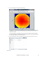
SAXSGUI User’s Guide (v2.05.02)
A Graphical User Interface for Visualizing, Transforming
and Reducing SAXS Images (as well as Limited Fitting)
by
Rigaku Innovative Technologies, Inc.
and
JJ X-Ray Systems ApS.
March 17, 2010
1.0 General Introduction................................................................................................................................. 2
1.1 What this manual does and does not.................................................................................................... 2
1.2 What SAXSGUI does .......................................................................................................................... 2
1.3 The underlying language: MATLAB and SAXS objects. .................................................................. 2
1.4 Supported MATLAB Versions: Version 7.10.0 (R2010a) ................................................................. 2
1.5 Installing SAXSGUI when you have a MATLAB license .................................................................. 2
1.6 Installing SAXSGUI when you do not have a MATLAB license ....................................................... 3
1.7 Starting and stopping SAXSGUI ......................................................................................................... 3
2.0 SAXSGUI windows ................................................................................................................................. 5
2.1 The SAXSGUI Window: Controls, menus, commands....................................................................... 8
2.1.1 The File menu................................................................................................................................ 8
2.1.2 The View menu ............................................................................................................................10
2.1.3 The Alter menu.............................................................................................................................11
2.1.4 The Calibrations menu..................................................................................................................11
2.1.5 The Reduction menu.....................................................................................................................16
2.1.6 The Quik_Enter menu ..................................................................................................................17
2.1.7 The Processing menu....................................................................................................................17
2.2 The Figure Window............................................................................................................................19
2.2 The Figure Window............................................................................................................................19
2.2.1 The Display menu.........................................................................................................................19
2.2.2 The Plot type menu.......................................................................................................................19
2.2.3 The Analysis menu .......................................................................................................................20
2.2.4 The Export menu ..........................................................................................................................22
2.2.5 The Batch Processing menu..........................................................................................................22
Appendix 1: Installing and running the SAXSGUI executable .....................................................................24
Appendix 2: Reduction: Spectra-by-Spectra or Pixel-by-Pixel .....................................................................25
Appendix 3: Auto Processing on the Molmet/Rigaku SAXS system............................................................26
Appendix 3: Auto Processing on the Molmet/Rigaku SAXS system............................................................27
Appendix 4: Masking With MATLAB MaskmakerGUI...............................................................................31
Introduction ...........................................................................................................................................32
Reservations and Acknowledgements ...................................................................................................32
Maskmakergui Details...........................................................................................................................33
Appendix 5: Constructing an artificial Flatfield ............................................................................................35
Appendix 6: Special Considerations for a Pilatus 300K................................................................................40
SAXSGUI User Manual v.2.05.02
1
1.0 General Introduction
1.1 What this manual does and does not
This manuals describes the windows and menus of SAXSGUI in some detail, focusing on
allowing users of SAXS data to navigate and make informed choices about actions within
the program. It does not teach or instruct the user on recommended practices for datareduction and analysis.
1.2 What SAXSGUI does
SAXSGUI reads SAXS images from files, allows you to explore the images visually, and performs various
operations and transformations, including full reduction of data as well as some basic fitting both IFT and
modeling. It also can be used to do some degree of batch processing multiple files.
SAXSGUI is provided under the GNU public license.
1.3 The underlying language: MATLAB and SAXS objects.
We’ve built SAXSGUI based on the MATLAB scientific programming language. We extended MATLAB
with a new class of objects, SAXS objects, designed to store, manipulate, and display SAXS images. Many
of SAXSGUI’s capabilities are also available at the MATLAB command line. Type
>help saxs
at the MATLAB command line for more information. If you want to see what an actual saxs-object looks
like type:
>A=getsaxs
and you’ll get a printing of the SAXS object created from the image file you choose.
1.4 Supported MATLAB Versions: Version 7.10.0 (R2010a)
SAXSGUI was originally developed for Matlab 6.5.0 (R13), which came out in 2002. Since then Matlab
has undergone some changes, including some very fundamental ones. We have struggled to keep the code
backwards compatible, but have from 2010 decided to support only the R2010a (7.10.0). Since the program
is available both as source code (for users with matlab licenses) and compile code (for users with no matlab
license), we believe this is acceptable. We believe that the code is indeed backward compatible till version
2008a (7.6.0).
1.5 Acknowledgements
SAXSGUI is in its present form mostly the result of efforts by JJ X-Ray Systems ApS and Rigaku IT Inc.
to provide an interactive software suite that was simple to start working with yet had all the necessary and
correct has developed since 2002, with input from many users.
Since its conception in 2001 the following people have contributed to the development of SAXSGUI, either
through contributons of algoritms, source code, or good ideas. Some of these people were paid, most were
underpaid, and many completely unpaid,
Scott Barton, now Molmex Scientific
Karsten Joensen, JJ X-Ray Systems Aps
Mike Degen, Rigaku IT
Milos Steinhart, Macromolecular Institute in Prague
Steen Hansen, University of Copenhagen, Life Sciences Department
Brian Pauw, Århus University, Chemistry Department
SAXSGUI User Manual v.2.05.02
2
2.0 Getting Started
2.1 Installing SAXSGUI when you have a MATLAB license
SAXSGUI requires MATLAB version 7.10.0 (2010a) or later.
Presently it comprises 3 toolboxes
¾
¾
¾
saxsgui -Containing the MATLAB files for manipulating saxs-data
BIFT - A MATLAB tool for performing Bayesian Inverse Fourier Transform on SAXS data
maskmaker – A MATLAB tool for creating masks to use only regions with good SAXS data.
And these 2 fitting model repositories:
¾
¾
saxsgui_ff_1d - a directory containing 1-d model functions callable by saxsgui
saxsgui_ff_2d - a directory containing 2-d model functions callable by saxsgui
In addition the following contributed toolboxes are distributed (with limited support)
¾
¾
sampledb - a toolbox for making a small database of saxs data – Contributed by Brian Pauw
mysacalibator - A toolbox for performing more detailed centering and calibration – Contributed
by Milos Steinhart
These toolboxes can be placed in the MATLABHOME/toolbox/ directory (or anywhere you like). They
should all be entered into the MATLAB path… (using the File->Set Path…menus). Press the save button in
the Set Path panel to ensure correct functioning also in later sessions.
You should also make sure that the setting in the SAXSGUI_settings.m file in the saxsgui toolbox are
correct. For example, make sure the variables fitfunction_dir_2D are defined as the actual pathnames of the
model file repository.
2.1 Installing SAXSGUI when you do not have a MATLAB license
The majority of this manual assumes you are running SAXSGUI with a MATLAB license. However for
users that do not want to invest in a MATLAB license, it is possible to run SAXSGUI on a Windows PC or
a Linux machine using an executable.
The executable is available on the www.saxsgui.com website. In order to run the executable, one needs to
download and run the saxsgui distribution package. For detailed installation and execution information see
Appendix 1. There may be some limited functionality on the executable. Please let us know if such is
discovered.
2.2 Starting and stopping SAXSGUI
Start MATLAB first.
Start SAXSGUI from the MATLAB command window, by typing
saxsgui
and SAXSGUI asks what image-file to open. Once you select an image, SAXSGUI displays it in
SAXSGUI’s main window. Use SAXSGUI menu commands and color scale controls to change the way
SAXSGUI displays the image, to transform the image, and to save or export images.
Stop SAXSGUI by closing the SAXSGUI windows or by closing the MATLAB command window.
SAXSGUI User Manual v.2.05.02
3
SAXSGUI can open a number of different file formats including:
•
•
•
•
•
•
•
•
MPA-files (binary and ASCII)
MATLAB data files (mat-files),
TIFF-files (including special Pilatus detector tiff-files)
Fuji IMG-files (which require also a inf file),
Bruker UNW- and GRFM-files,
Hecus CBM-files as used at Risoe National Laboratory,
EDF files
Rigaku IMG-files (RADIA format – Rigaku image plates)
Files from Rigaku are usually in MPA format, Fuji IMG-files or Rigaku IMG files
MAT files must contain a SAXS image saved from SAXSGUI or from the MATLAB command window.
Tiff files from Pilatus 100K and 300K have special read-in filters to handle the dead stripes on the detector
Advanced tip: to open a SAXS image that you have created in the MATLAB command window, as
opposed to an image saved in a file, type saxsgui(image_name).
SAXSGUI User Manual v.2.05.02
4
3.0 SAXSGUI windows
SAXSGUI interacts with you through several windows, for example
•
•
•
•
•
•
•
•
The SAXSGUI window
The Fatpix window
The Reduction Parameter window
The Data Reduction and Averaging window
The Figure windows
The Interactive Batch Window
The Maskmaker window
The Flatfield construction window
In the following, a brief gallery of these windows will be shown, followed by a more detailed presentation
of available menus.
The main SAXSGUI window displays images and controls image visualization and transformation.
Tip: Resize and move the SAXSGUI window to suit your needs. Maximize the window size to see the
most detail and largest region. Use the View/Zoom command, too, but read directions for it, elsewhere in
this document, first.
The fatpix window shows individual pixel intensities from
wherever you click on the main SAXSGUI image. You can
invoke it under the SAXSGUI window View menu.
Tip: Expand the fatpix window to see more pixels at once.
SAXSGUI User Manual v.2.05.02
5
The Reduction Parameter window displays images
and controls image visualization and transformation.
It is also the window from which maskmaker and can
be launched and artificial flatfields created.
Tip: Use the save and load configuration to save
typical reduction parameters, so you don’t have to
enter these every time.
Data Reduction and Averaging Window allows the user to choose how to perform the averaging. The
user can choose the desired q-range and azimuthal range on the image to the right. Also the various
reduction parameters chosen in the Reduction channel can be toggled on and of.
Tip: Use the “same as last
buttons” to save time
when analyzing similar
images. Also opt whether
to choose to plot in a new
plot area or on top of the
last figure window.
Figure windows display the results of averaging radially or
azimuthally.
Tip: Use the menus below the Display and Plot Type menu to
change the axis scaling and produce standard SAXS plots. If
more advanced image manipulation is required, one can
invoke the standard Matlab figure menu by asking for it under
the Display menu.
Tip: More than one curve can be plotted on any one graph.
SAXSGUI User Manual v.2.05.02
6
Batch (Time Series) window is spawned through the
figure window’s Batch menu, and allows one to reduce
any number of files identically to the way the plot in
the figure window was reduced. This works well for
uncomplicated reductions, but not so well if the
transmissions or background files change.
Tip: Add up to 5 formulas to calculate special values
for the reduced file…for example something like
“integrated area”
Maskmaker window is spawned through the Edit Reductions File Menu, and is used to create a mask for
the reduction of images. Pixels inside or outside various geometrical figures can be selected for exclusion.
See Appendix 4 for examples of how to use the maskmaker tool.
Tip: Be sure to save the RONI (Region of Non-Interest), so that it can be used later for easy maskmaking.
Flatfield maker window is also spawned
through the Edit Reduction window. It is used
for constructing pseudo flatfields based on real
low intensity flatfields and high intensity nonflatfields. This tool was created as an alternative
to the often time-consuming flatfield
measurements, albeit a clearly inferior
alternative. See the SAXSGUI Demos for an
example of how to use the Flatfieldmaker
window.
SAXSGUI User Manual v.2.05.02
7
3.1 The SAXSGUI Window: Controls, menus, commands.
The SAXSGUI Window is the entry point into the SAXSGUI programs and panels. The version of
SAXSGUI is displayed in the top left window name
3.1.1 The File menu
This menu contains commands for reading and writing files, as well as for setting central SAXSGUI
preference.
¾ Open...
Opens an image file, replacing whatever image SAXSGUI is displaying. If you want to save
changes you have made to the previous image, use the Save command before opening a new file.
¾
Open from SPEC file
¾
Combine and Open
¾
Name...
¾
If you have specified that you are working in a SPEC environment in the SAXSGUI_settings.m
file then this menu will be available. It opens allows you to open an image file that is listed in a
SPEC log file. Otherwise it works as open…
Prompts you to choose a number of images, which will then be combined (pixel-by-pixel) and
opened. If the files contain information on exposure time, the final image will contain information
on the combined exposure time.
Give the SAXS image a new name. The name appears above the image display in the SAXSGUI
window. The Save command saves this new name with the image.
Save image as…
Save the SAXS image with the changes you have made. SAXSGUI prompts you for a file
location and name. SAXSGUI saves the image-pixel values as either a MATLAB data file with a
MAT-file name extension, or a tiff file (8 or 16 bit), or a text-file with ASCII-characters. When
saving as a MATLAB-file, additional information about the image is also saved. In this case, you
reopen the file later with the Open command to continue where you left off.
If saved as text data files the following formats can be chosen
¾ x,y (left) image…
Export the SAXS image in its x,y form (not polar transform) to a text data file. SAXSGUI
presents a dialog window where you specify the format of the exported data (see below), what
coordinate range of the image to export, and how many digits to print past the decimal point
for all numbers. After you make selections, a file selection window allows you to specify
where to place the exported text.
¾ polar (right) image…
Same as x,y above for the polar transformed image, the right-hand image in the SAXSGUI
window.
SAXSGUI User Manual v.2.05.02
8
¾
Export Window
Export the whole SAXSGUI window to either a TIFF,
JPEG, PDF or a matlab figure file.
¾ SAXSGUI Preferences
¾
¾
¾
Set SAXSGUI Preferences
Set the SAXSGUI preferences using the panel seen to
the right. The preferences pertain to look-up-data
required for the various auto-calibration features, the
auto-centering features, the default smoothing
paremeters, the default zinger parameters, the default
averaging parameters and the orientation of read fuji
image plates.
Use Default Preferences
Close
Closes the SAXSGUI window.
SAXSGUI User Manual v.2.05.02
9
3.1.2 The View menu
This menu affects the way SAXSGUI displays images.
Most of these commands are toggles which turn certain image viewing features on and off. When the
feature is on, a check mark appears beside the command in the menu.
¾
Log intensity (toggle)
Display the common logarithm of intensity values. This changes the way colors are mapped to
intensity values. The color scale controls disappear, while you view log intensities. Choose this
command again to display linear intensity values and restore the color scale controls.
¾
Grid (toggle)
¾
Zoom (toggle)
Display grid lines across images. Choose this command again to remove the grid lines.
Turn zoom control on (see below). Choose this command again to toggle zoom control off.
SAXSGUI may turn zoom off automatically after some other commands.
Pointer action
Effect
left click
Zoom in at the pointer position.
right click
Zoom out.
drag
Zoom to the dragged area.
double click
Zoom out to the full image.
¾
¾
¾
¾
¾
¾
Crosshairs and coordinates (toggle)
Turn on full-window crosshairs that follow your pointer. Turns on x,y coordinate labels that show
the current pointer position in terms of each image’s axes coordinates. Choose this command
again to toggle crosshairs and coordinates off.
Projection along Line(toggle)
Brings up a figure and a line in the image. The figure shows the pixel-values along the line. The
line may be moved around by using the left-button of the mouse to move the edges. Known Bug:
Apparently it appears that right-button clicking the mouse kills the functionality.
Color map…
Choose a different color map to display image intensity values. The default map is ‘jet’. Those
used to Bruker software may prefer ‘hot’, while Rigaku software will prefer jet.
Fatpix
Open a fatpix window that zooms in to the x,y (left-hand) image, showing individual pixels and
labeling each pixel with its intensity value. The fatpix window updates the pixel display whenever
you click on the left image in the SAXSGUI window, showing pixels in the region of your pointer.
Enlarge the fatpix window to show more pixels at a time. Shrink the fatpix window to make
updates speedier. Close the fatpix window when you finish with it.
Image history…
Open a window showing the history of the currently displayed SAXS image. Close the history
window when you finish with it. This history also contains the intensity in the image.
MATLAB menus (toggle)
Add standard MATLAB figure menus to the menu bar. Choose this command again to remove the
MATLAB menus from the menu bar.
SAXSGUI User Manual v.2.05.02
10
3.1.3 The Alter menu
¾ Clean Up
¾
¾
Zinger Removal
This menu item applies a filter to the 2D data that will remove any part of the image that look
like a Zinger. A Zinger is usually observed in lengthy exposure with solid state imaging
detectors and are caused by cosmic radiation interacting with the detector to create a large
localized intensity. The characteristics of the generic zingers should be given in the
SAXSGUI gui preferences accessible from File menu of the SAXSGUI window. The data in
the “zinger region” is tagged as if it were to be masked out in the averaging routines. Zinger
removal would also remove single madly firing pixels.
Bad Pixel Removal
This menu applies a filter to the 2D data that will remove any single madly pixel. In fact it
looks for up to 50 such pixels, with excess intensity. If such pixels are found they and the
nearby pixels are tagged for later masking out.
¾ Smooth
¾
¾
Gaussian filter…
Smooth by applying a Gaussian FIR (finite impulse response) filter to the image to remove
higher frequency features. This reduces the noise level of the image, enabling easier
visualization of image features and possibly better symmetry computations (centering,
elliptical normalization). You specify the size of the filter (size of convolution box) and the
standard deviation of the Gaussian curve to use (i.e. the standard width of the distribution in
pixels). Smoothing conserves overall intensity.
Undo smoothing
Restore the unsmoothed image. SAXSGUI maintains the results of certain interim operations,
such as background subtraction, centering, and calibration.
¾ Rotate
¾
Specify Rotation
Enter the desired anti-clockwise rotation (in degrees). Rotates around the defined center.
¾ ListMode
¾
Alter Time Slice
MPA-files may be recorded in ListMode, which is a mode in which the pixel position, and
time is recorded for each individual photon. These files are loaded and displayed with all of
the available photons. This menu item allows one to create an image with only a subsection of
the photons. Tip: This could be used to look at a complete reaction, the listmode recording
from the beginning of the experiment to the end. One could then alter the time slice to look at
the intensity before the reaction and after the reaction.
3.1.4 The Calibrations menu
This menu handles all of the calibrations of the images: q-calibration, centering, absolute intensity
calibration and even the homegrown “error”-calibration
¾ Same As Last
A quick press menu for doing the exact same calibration as the previous image. The calibration is
lost when MATLAB is closed.
¾ Q-Calibration
¾
¾
Q-Calibration: Same as Last
A quick-press menu for using the last q-calibration. Tip: Start your session by calibrating with
a SilverBehenate Sample and then use this “Same as Last” menu on the following images.
Q-Calibration: Using Ag-Behenate
Quasi automatic q-calibration with a Silver Behenate image showing a full ring. The user is
requested to click on three points on the 1st order ring. SAXSGUI then calculates the center
and diameter of the ring thereby allowing the calculation of the appropriate q-calibration in
the x- and the y- direction. Tip: If you are doing WAXS you may not have the first order ring
SAXSGUI User Manual v.2.05.02
11
¾
¾
in the image. In this case you can press on n’th order; go into manual calibration and change
the “q-value for line” to n times the value of the first order (n times 0.1076 Å-1).
Q-Calibration: Using Ag-Behenate by partial ring
Quasi-automatic q-calibration as above, however this version is used when there is only a
partial ring available. It is less robust than the full ring q-calibration above.
Q-Calibration: Manual Calibration
This menu brings up a small input panel, where you can put your calibration information. One
can choose to either use the mode where one has a image with a calibration ring, whose pixel
diameter one can enter, or by system geometry where one enters the pixel sizes in millimeters
and the distance from the sample to the detector. One choose the method by clicking on the
radio buttons at the top.
¾
Q-Calibration: Mysa Calibrator
This brings up a calibrator tool contributed by Milos Steinhart in Prague. This tool provides
the user with more control of the q-calibration and centering. The user can choose which
regions and which pixel intensity levels to include in the calculation of the best fit calibration
rings. This tool is therefore helpful in the less straightforward cases of centering and qcalibration (partial rings, offsets etc)
¾
Q-Calibration: Save Calibration:
Save the calibration values in a file. This is necessary if you want to use the file-based autoprocessing feature, but also useful if you want to revisit the dataset.
Q-Calibration: Load Calibration
Load the calibration values from a previously saved calibration file.
Q-Calibration: Uncalibrate
Remove calibration data from the image. Display in pixel coordinates again.
¾
¾
SAXSGUI User Manual v.2.05.02
12
¾ Center
This menu item allows you to select the center in one of may ways. Once you have specified the center
for the SAXS image, SAXSGUI displays a lower resolution polar transformation in the right side of
the SAXSGUI window, using the same color mapping as the original image.
¾
¾
¾
¾
¾
¾
¾
¾
¾
¾
Center: Same as Last
A quick-press menu for using the last center calibration. Tip: Start your session by calibrating
with a sample with a well defined center, for example Silver Behenate Sample and then use
this “Same as Last” menu on the following images.
Center: Auto-Compute Center
This unique little feature, calculates the best fit center based on quick optimization routine.
Most of the time it does a very good job. Simply activate the menu. Tip: If this routine is
having trouble finding the correct center, you may help it by first “clicking a center” to get an
approximate center and then running the routine again. Or you may need to change the
“mask” radius in the SAXSGUI preference…especially if the central region is very intense
and extended. However, the need for this should be very infrequent.
Center: Compute Center by …
Allows quasi-automatic centering based on images with either a ring, a partial ring, 4 arcs or 2
arcs.
Center: Direct Beam Centering
Some systems will allow the direct beam or an attenuated direct beam to strike the detector
without a beam stop and use the resulting image to determine the beam center. This menu
item established the center position based on a 2-dimensional peak-fit to such an image.
Center: Manual
Allows you to manually enter the center coordinates. Or simply take a look at what
coordinates are presently used.
Center: Mysa Calibrator
This brings up a calibrator tool contributed by Milos Steinhart in Prague, that can be used for
both q-calibration and centering. This tool is described in more detail in the q-calibration
section of this document (Section 2.1.4)
Center: Enter Coordinates
This brings up a small panel that will allow you to enter the center coordinates manually.
Center: Click to center
Activating this menu brings up a set of crosshairs. When you click on a point in the image the
corresponding coordinates are entered as being the center. This feature is best used with an
image that is somewhat zoomed or at least fills the whole screen.
Center: Save Center…
Save the center coordinates in a file, so you can load it in later sessions. You need to do this if
you want to use the file-based Auto-processing function
Center: Load Calibration
Load center pixel coordinates from a MATLAB data file and apply to the current image. The
data file may have been created by the ‘save center’ command or may contain a centered
SAXS image saved as a mat-file.
SAXSGUI User Manual v.2.05.02
13
¾ Absolute Intensity Calibration
The absolute intensity calibration relies on the fact that the difference between the data on absolute
scale and relative scale is only a factor of some magnitude (SAXSGUI refers to it as the Absolute
Intensity Factor) and the assumption that the source is stable enough that intensity calibrations
established for one image are acceptable for later images. In other words the program does not
explicitly allow for measurements requiring “an intensity monitor”. However, for most laboratory
sources this is not a problem and intensity calibrations with a secondary standard like Glassy
Carbon can be done frequently.
¾ Absolute Intensity: Same as Last
A quick-press menu for using the last Absolute Intensity Factor.
¾ Absolute Intensity: Enter Manually
Enter the “Absolute Intensity Factor Manually”
¾ Absolute Intensity: By water
This brings up a small panel, which
essentially is a tool for doing primary
calibration using water as a a priori
standard. The tool requires that the
active image in SAXSGUI is the image
taken of water within a holder, and that
you also have available an image taken
of the holder without water (empty
holder). The tool then requires that you
fill in the panel seen below at least with
the information on transmissions and
file name. When pressing Calculate it
will calculate the actual sample
thickness and the absolute intensity
factor. Note: This default operation for
this tool is at CuKα-radiation. If other
energies are to be used, the attenuation
length of water should be changed
according in the SAXSGUI preferences
(in the File Menu of the SAXSGUI
window).
¾ Absolute Intensity: By Glassy Carbon
This menu item uses a Glassy Carbon measurement as a secondary intensity standard. It
assumes that the Glassy Carbon image is the active image in the SAXSGUI window. It also
assumes that the particular piece of glassy carbon, has previously been calibrated (for
example against water) and that the calibration value has been entered into the SAXSGUI
preferences.
¾ Absolute Intensity: Save Calibration
Save the center coordinates in a file, so you can load it in later sessions.
¾ Absolute Intensity: Load Calibration
Load the Absolute Intensity Factor from a MATLAB data file and apply to the current image.
The data file may have been created by the ‘Save Calibration” menu
¾ Absolute Intensity: Uncalibrate
Remove the Absolute Intensity Factor from the data.
¾ Absolute Intensity: What’s this
Brings up a text box with a very brief explanation.
SAXSGUI User Manual v.2.05.02
14
¾ Error Calibration
This menu allows you to apply a normalization factor to the standard deviations calculated by
SAXSGUI. Since SAXSGUI assumes that your pixel values are in units of “photons per pixel” (as
is true with photon counting detectors) it calculates the expected errors accordingly. However,
when using CCDs and Image Plates the units are different and the calculated errors are
consequently completely wrong. In order to obtain correct error estimates, one therefore needs to
apply a correction., which we assume to be a simple factor: The Error Normalization Factor.
While it is possible to calculate the correction from detector specifications, the SAXSGUI
approach relies on computing the Error Normalization Factor from the observable statistics in an
actual image (ideally a flat field image).
¾ Same as last
Allows you to quickly apply the same error normalization factor as the previously calibrated
image. The calibration is lost when MATLAB is closed.
¾ Compute
To compute the Error Normalization Factor, use an image which has a large flat region. After
choosing this menu item you are prompted to define a rectangle. The program then calculates
the actual error normalization factor, based on a calculated mean and observed statistical
distribution of pixel values. For photon-counting detectors (gas detectors and Dectris Pilatus
detectors)-detectors the value should be close to 1.
¾ Manual
Here one can enter the parameter manually.
¾ Uncalibrate
Remove error normalization calibration data from the image
¾ What is this?
Briefly explains what this menu can be used for.
SAXSGUI User Manual v.2.05.02
15
3.1.5 The Reduction menu
Data reduction is crucial to obtaining data that you can fit and model. Examples of data-reduction are
background subtraction, flood field correction, absorption corrections, and absolute scaling. Data-reduction
can be done either directly on the 2D images themselves, or on the 1D spectra often obtained by averaging
radially or azimuthally (See Appendix 2)
This menu allows you to specify which reduction parameters are to be applied to the image, as well as
stating whether you want to see them applied interactively or you can wait till later (for example when
averaging)
¾ Same as last…
Allows you to quickly apply the same reduction parameters as the previous image. This information is
lost when MATLAB is closed.
¾ Edit Parameters
This Opens up a panel, where you can
specify which reductions are relevant.
This panel itself has a “File”-menu
where you can
¾ Save the information contained in
the panel
¾ Load previously saved information
from the panel
¾ Create Mask for opening up the
program maskmakergui where you
can create a mask for the data.
¾ Construct an artificial flatfield
from low intensity flatfield
measurement and high intensity
non-flatfields.
One can see that you can choose to
apply one or more of the reductions and
corrections by activating the buttons on
the left, after which one should enter
the appropriate data in the form of
numbers or filenames. When the apply button is pressed the information in the SAXSGUI window is
updated. This reduction window can be left open if several data sets are to be analyzed.
At the bottom of the reduction panel one can see 5 configurations, which each can store and recall
separate sets of reduction parameters.
¾
Clear Parameters
¾
Apply when averaging (1D)
Removes all the reduction information from the image.
This is the default mode where reduction parameters are recorded, but not yet applied to the data that is
shown in the 2D images. This puts the least strain on the computer CPU and graphics card.
¾ Apply interactively (2D)
The reduction parameters are recorded and applied to the 2D images shown. This is necessary if one
wishes to do save the reduced 2D data for use in another program.
¾ What is this?
Briefly explains what this menu can be used for.
SAXSGUI User Manual v.2.05.02
16
3.1.6 The Quik_Enter menu
¾
As last
Essentially performs “Error Calib->Same as last” ,“Calibration->Same as last”, “Center-> Same as
last” and “Reduction->Same as last”, one after the other and thus becomes a one-button complete data
preparation.
¾ What is this?
Briefly explains what this menu can be used for.
3.1.7 The Processing menu
Most SAXS data analysis from 2D images will make use of 1D projections of the data. Either projection
along the momentum transfer axis, or the azimuth angle.
¾
Averaging (1D spectra)
Activating this window brings up the averagex plotting window, where you can specify exactly how
you want the data averaged and reduced.
From the screen dump below, you can see that it is possible to:
¾ choose how many points (bins) you want in your 1D spectrum, and whether you want the
distribution of these bins to be Linear or Logarithmic.
¾ specify whether reduction should be performed pixel-by-pixel (which requires correction data with
good statistics) or spectra-by-spectra. (For more information on the difference see appendix 2)
¾ specify plots of azimuthally averaged intensity vs. momentum transfer or average intensity vs.
azimuth angle.
¾ indicate exactly which reductions you would like to apply.
¾ specify the “the area” that you want to average over, either by entering values or by pointing and
dragging a rectangle in the right-hand image.
¾ Choose to press the “same as last” buttons if all you want to do is repeat the previous averaging
SAXSGUI User Manual v.2.05.02
17
To perform the averaging and obtain the data in plotted format, you can either press the “New plot” button
to obtain a new figure window, or the “Add plot” to add the result to the last visited plot window.
Known Bugs:
1) As seen in the above screen-dump you can choose reduction type, even though no reductions have
been specified previously in the reduction panel. Solution: These should be disabled. Severity:
cosmetic
¾
AutoProcess
The previous menus are all very useful when you are operating in a very interactive
mode…calibrating, centering etc etc….. But if you are taking many SAXS images with very similar
parameters, requiring very similar processing and similar outputs, then perhaps it is time to consider
auto-processing. Also, if you are used to working with batch files and configurations files, the
autoprocessing may appeal to you more than the GUI approach.
The present version of the Auto-Processing only works for Molmet/Rigaku data (mpa-format) that has
been taken with LabView SAXS control program – with some care taken to get the right information
into the info-file. (Other users can contact JJ X-Ray Systems to discuss if it is feasible to extend
support to other setups).
The Auto-processing requirements are described in greater detail in Appendix 3, however in brief it
allows SAXSGUI to access
1) a configuration file the “AP Setup” file, with parameters that describe the setup, the averaging
instructions and the output instructions
2) the info-file that is saved when data is saved using the Labview program. This info-file would
need to include information specific to the sample such as sample thickness, sample transmission,
empty holder file, empty holder transmission etc
and use this information to proceed as far as the instructions indicate.
The Auto-Processing sub menu has the following sub-menus:
¾ AP Setup
This prompts for a AutoProcesseing configuration file
¾ AP Single File
This will prompt for a single mpa- file and perform the data-reduction and processing requested in
the configuration file. The latest saved configuration file is always used. If no configuration file is
requested this menu will prompt for a configuration file first.
¾ AP Multiple Files
This will prompt for a list of mpa-files and perform the data-reduction and processing requested
in the configuration file. The latest saved configuration file is always used. If no configuration file
is requested this menu will prompt for a configuration file first.
SAXSGUI User Manual v.2.05.02
18
3.2 The Figure Window
Here you see the azimuthally averaged
intensity vs. momentum transfer for Silver
Behenate; the plot has 200 linearly
distributed points. The leftmost peak is
actually not a peak, but rather a result of the
beam stop blocking intensity for the smallest
momentum transfers.
In the top of the figure, you’ll see several
menu-items, which shall be described in
more detail below.
Note: if you desire the standard Matlab
figure window menus, (for example to
manipulate the axis in detailed ways) you
can toggle the “Display -> Matlab Menus”
menu.
3.2.1 The Display menu
The menu allows for rapidly changing the axes between logarithmic and linear scaling, as well as toggling
error bars on and off. There is a bit of difference between available features for intensity vs. momentum
transfer or intensity vs. azimuth angle, as shown in the table below:
Availability of axis scaling and
plot content
Linear-Linear
Logarithmic –Linear
Linear – Logarithmic
Logarithmic – Logarithmic
Toggle Display of Error bars
Toggle Standard Matlab Menu
I vs. momentum transfer plots
For Intensity vs. azimuth plots
Available
Available
Available
Available
Available
Available
Available
Not Available
Available
Not Available
Available
Available
The menu also provides a zoom menu item that allows you to zoom in on region of the figure that may
interest you.
2.2.2 The Plot type menu
Many different types of plots have shown their use in SAXS data presentation. A couple of these are
available under this menu.
Availability of axis scaling and
plot content
I vs. q
Ln(I) vs. q2
1/I vs. q2
I * q4 vs. q
I * q2 vs. q
Guinier Plot
I vs. momentum transfer plots
For Intensity vs. azimuth plots
Available
Available
Available
Available
Available
Available
Available
Not Available
Not Available
Not Available
Not Available
Not Available
Note: We will gladly add others, if it makes sense and is requested.
SAXSGUI User Manual v.2.05.02
19
3.2.3 The Analysis menu
This menu item contains a number of possibilities for analyzing the data ranging from a simple statistical
analysis to fitting a few generic models, to multiparameter fitting of standard and potentially user-defined
function and finally to a very nice little Inverse Fourier Transform.
¾ QuikStat
Allows you to define a region of the curve and the provides you with information on the q-range, the
intensity range and the integrated intensity of the region you selected.
¾ QuikFit
This menu provides the opportunity to fit a userdesignated region of the curve to one of a large
number of very standard models organized in
main themes. The fitting routine does not allow
one to enter starting parameters, but attempts to
calculate the starting parameters based on userclicks on the graphs. The optimization scheme is
a Downhill Simplex Optimization. The themes
and models available are given in the table
below.
Fitting Themes
PeakFit
Brief description
Fits to various type of
peak-models
PorodFit
Fit Simple Porod
Models
Fits to Guinier Model
Fits to a powerlaw
function
Available
GuinierFit
FractalFit
OtherFit
Fitting Models
Gaussian Peak with Linear/Slope Background
Gaussian Peak with Expon./Spline Background
Lorentz Peak with Linear/Slope Background
Lorentz Peak with Expon/Spline Background
Pearson VII Peak with Linear/Slope Background
Pearson VII Peak with Expon/Spline Background
Double Pearson Peak with Expon Background
Porod Model
Porod Model with Background
Guinier Model
Fractal Dimension/Power Law
Fractal Dimension/Power Law with background
Combined Guinier-Porod
Combined Guinier-Porod with background
SAXSGUI User Manual v.2.05.02
20
¾
FullFit
This menu item starts up a panel intended for bounded optimization of various standard SAXS related
models. The models are all provided as MATLAB functions in the saxsgui_ff_1d directory, they have
been adapted from the published articles of Jan Skov Pedersen. The program uses a Downhill Simplex
optimization routine and requires one to specify starting values and bounds for all parameters as well
whether one wants to fit the parameters or not. The panel layout and default provided models are seen
in the figure below.
Tip: It can sometimes be difficult to find starting parameters that will result in a reasonable fit. To
“play around” you can enter Start values and press the Calculate button, to see how the calculated
curve compares.
¾ Bayesian IFT
The menu item invokes a Bayesian
Inverse Fourier Transformation
program called BIFT. The program
is based on a Bayesian approach to
IFT of SAXS data first described
by S. Hansen, now at the
University of Copenhagen – Life
Sciences Department. BIFT has
been coded by K. Joensen, JJ XRay Systems ApS and the user is
referred to BIFT program manual,
supplied separately.
SAXSGUI User Manual v.2.05.02
21
3.2.4 The Export menu
The data in the plot window SAXS data can be saved in a couple of formats:
•
•
•
Comma separated dataformat (*.csv), with no header lines
As PHD-files (Glatter format)
As Rad-files (Risø format)
Only one curve can be saved to each file.
In the future there may be several options for exporting format, but presently all data from a single plot are
exported to a single file in X,Y, ΔY in 3 columns.
3.2.5 The Batch Processing menu
SAXS data may at times consist of a whole series of images all to be reduced in the same way. SAXSGUI
currently provides 2 ways to approach this. The first is the interactive Batch processing by Graphical User
Interface (template-based) way which allows you to reduce a large number of files in the exact same way
you have done for the curve in the figure window. The second is the AutoProcessing way which uses
reduction information in a batch file and ca be accessed from the main SAXS gui window. The Batch
Processing menu in the Figure window allows you to start the interactive way or to save a batch file that
corresponds to the way the data in the figure was reduced and can thus be used as a starting point for the
AutoProcessing.
¾
Save Template AP-file
This saves a file that can be used either directly as input to the AutoProcessing routines (started from
the main SAXSGUI window or from altered to correspond to actual alternate Autoprocessings.
¾
Batch by Gui: TimeSeries
At this time Batch reduction of Time
Series is available through the Time
Series sub-menu. When this sub-menu
is activated, the user is requested to
click on the line-graph that is going to
be the “template” for the rest of the
Batch evaluation. A panel controlling
input to the Batch routine is then
opened (see below)
In the panel you can:
1) Choose the files you want to
batch process.
2) Choose the sample
transmission (Actually the
program knows this already
but we just have to figure out
how to get it reproducibly into
the text-field in the panel). If
you do not care what the sample transmission is, leave it at 1. …which will of course upset
any corrections, relying on the correct transmission for example “Empty holder” subtraction
3) Choose the sample thickness…
4) Choose how the x-axis of the time series should be constructed
a. By just incrementing 1-2-3 etc
b. By using time recorded in the data of the header
c. By using the time that the data file was saved (or altered last)
SAXSGUI User Manual v.2.05.02
22
The latter may be necessary if particular headers don’t carry “saved time” information as is
the case with most tiff-files.
5) On the bottom you’ll see the output options which are:
d. Save the 2D data (as jpegs)
e. Save the 1D averaged data (as jpegs)
f. Save the reduced data to separate ASCII files (comma separated)
g. Save the reduced data to one large ASCII file (comma separated)
h. Save x-y data or x,y, Δ y data
If saving ASCII data, the reduced data will be saved in a file with a name exactly the same as
the original data name… only with a tag added…You must specify this tag in the “Descriptive
Tag” field.
6) Once you have chosen the files, the “start batch” button is enabled and you can start the batch
processing by pressing it.
Advanced Batch Feature
The Special Analysis section of the table allows you to enter up to 5 MATLAB expressions, which
will be evaluated for each data-file. The expression must be composed of strings that could be
recognized by MATLAB as regular MATLAB expressions. X and Y are the array-variables
holding the data from the plot.
At the end of the batch process the result of any one expression (which should always be a single
figure) will be plotted as function of time and also saved to an ASCII file.
Examples of expressions could be:
Example 1:
sum(Y(X>0.02) & (X<0.48))
which calculates the sum of all the plot values where 0.02<X<0.48, essentially “area under the
curve”. Such a function could be used to integrated peak intensity evolved over time.
Example 2:
max(Y(X>0.02) & (X<0.48))
which calculates the maximum value in the same region as Example 1
SAXSGUI User Manual v.2.05.02
23
Appendix 1: Installing and running the SAXSGUI
executable
Components:
The executables are distributed from the www.saxsgui.com website. They are distributed in packages
containing the saxsgui program, the matlab components and various needed and recommended files.
The distibutable-packages are available for download at:
http://www.saxsgui.com/saxsgui_win32_pkg.exe
http://www.saxsgui.com/saxsgui_win64_pkg.exe (not yet)
and
http://www.saxsgui.com/saxsgui_lin32_pkg.zip (not yet)
There are also manuals available at
http://www.saxsgui.com/manuals.zip,
and demo data available at
http://www.saxsgui.com/data1.zip
http://www.saxsgui.com/data2.zip
In windows, once you have downloaded the package, you can run it, and the installation of the necessary
components will take place.
In linus you should unzip the package into the directory you want to run SAXSGUI from and then run the
MCRInstaller followed by SAXSGUI. The additional files should all be located in the same directory as the
saxsgui_platform program. These are
o
o
o
saxs_preferences.txt
saxs_preferences_default.txt
standard_fitfunctions.mat
SAXSGUI User Manual v.2.05.02
24
Appendix 2: Reduction: Spectra-by-Spectra or Pixel-byPixel
SAXGUI allows you to reduce your averaged data in 2 ways:
¾ Pixel-by-pixel and
¾ Spectra-by-spectra
The reduction schemes are graphically represented on the next page for a case where reduction consists of
subtracting the signal from an empty sample holder from that of a filled sample holder.
It is immediately clear that if Reduced 2D data is required (for example for 2D modeling) then the Pixelby-Pixel approach has to be used.
However, if only 1D averaged data is required then the Spectra-by-Spectra approach can be used,
especially when the data has poor statistics. One can even see this effect on the example on the next page.
For this example it is not a huge difference, but it is a discernable difference; the Pixel-by-Pixel data is
more noisy.
Note: One important case where Spectra-by-Spectra should be considered is if the flatfield image does not
have significant statistics. In this case the deviation of intensity distribution deviates from a gausssian
distribution and thus makes a significant difference between the two approaches.
The advantages and disadvantages are summed up below:
Technique
Pixel-By-Pixel
Advantage
¾ Can obtain 2D images
¾ Can create good pictures for
Spectra-By-Spectra
¾ Robust
¾ Work well with typical
Disadvantages
¾ Not so robust, since pixels
with 0 counts create trouble
¾ Caution when using noisy
data.
¾ Fails when using flatfield
with poor statistics (many
zeroes for example)
¾ Cannot obtain 2D images
SAXS data (noisy, countrate-limited
SAXSGUI User Manual v.2.05.02
25
Pixel-by-Pixel Reduction
-
=
2D-Output
1D-Output
Spectra-by-Spectra Reduction
-
=
SAXSGUI User Manual v.2.05.02
1DOutput
26
Appendix 3: Auto Processing on the Molmet/Rigaku
SAXS system
Auto-processing on the Molmet/Rigaku SAXS system in implemented through the 2 key files that can be
prepared either by the user and/or by the LabView SAXS program.
The first file is the info file generated by LabView SAXS control program every time an image is saved by
the LabView program. An example is seen below:
SamplePosition = 5,6
SamplePositionMM = 89.524,69.959
Sample Description = SAMPLE IN CAPILLARY
Username = SANSE
Date = 5/8/2008 4:40 PM
Trans Factor = 1.000000
LiveTime = 300
RealTime = 300
Background file =
Intensity file =
Flatfield file =
Dark count file =
Comments =
PhotoDiode = 246.566E-12
Ones sees that there is a lot of space for putting in information that is pertinent to the sample. If one
constructs an appropriate script, the generated info-file could look like this:
SamplePosition = 0,1
SamplePositionMM = 89.524,69.959
Sample Description = POS1
Username = SANSE
Date = 11/8/2008 10:20 PM
Trans Factor = 0.302
LiveTime = 60
RealTime = 60
Background file = 'C:\Data\Yale\Solution 850 mm\000066.mpa'
Intensity file =
Flatfield file =
Dark count file =
Comments =
PhotoDiode = 730.632E-12
Although this is better, the trained eye would see that there is presently no room for sample thicknesses,
background file transmissions and other parameters that are specific to the sample being measured….so to
circumvent this present limitation in the info file,we use the Comments spot:
SamplePosition = 0,1
SamplePositionMM = 89.524,69.959
Sample Description = POS1
Username =
Date = 11/8/2006 10:20 PM
Trans Factor = 0.245000
LiveTime = 60
RealTime = 60
Background file = 'C:\Data\000066.mpa'
Intensity file =
Flatfield file =
Dark count file =
Comments = 'sample_thickness=0.1 ; background_transmission=0.15; temperature=30'
PhotoDiode = 730.632E-12
The comments string should all be on the same long line and enclosed in ‘
The parameters are keywords and must be written exactly as seen. The order doesn’t matter
SAXSGUI User Manual v.2.05.02
27
The user can either construct the LabView script so that the comments files are generated by the script or
add them at a later time.
The more general parameters for the reduction are provided in an Auto Processing configuration file as
seen here:
% See full description at bottom of file
%Reduction Info: if it has a value it will be included in the reduction
matlab_center_file = 'C:\Data\Kavala\center_mr' %REQUIRED: must be created in SAXSGUI
matlab_calib_file = 'C:\Data\Kavala\qcalib_mr' % REQUIRED:must be created in SAXSGUI
%flatfield_filename= 'C:\Data\Fe55FloodField#1\2_4_40kV_1_5kV_11_15V.mpa'
abs_int_fact= 37.6
mask_filename= 'C:\Data\Kavala\mask_ads'
empty_filename='C:\Data\Kavala\empty.mpa' % should be included in the info-file
empty_transfact=0.1027 % should be included in the info-file
%solvent_filename='C:\000066.mpa'% should be included in the info-file
%solvent_transfact=0.23% should be included in the info-file
%solvent_thickness=0.104% should be included in the info-file
% Generic Info
error_calib = 1
% Should be 1 for Molmet gas detectors
%darkcurrent_filename= 'C:\Data\000067.mpa'
%normally so low not required
%readoutnoise_filename= 'C:\Data\000068.mpa'
%not required for Molmet detectors
zinger_removal= 0
%not required for Molmet detectors
%Averaging Info - This section is optional- Comment out to "stop" before averaging
do_average= 1
% 1=do averaging, 0= do not do averaging
I_vs_q = 1
% 1=do I_vs_q, 0=do I_vs_phi. Default is I_vs_q
phistart = 0
%azimuthal start angle in degrees
phiend = 360
%azimuthal end angle in degrees
qstart = 0.001 %radial start value
qend =0.35
%radial end value
xaxis_type= 'lin' % can be 'lin' or 'log'
num_xpoints= 400 % number of points on the x-axis
reduction_type='s' % can be default='s'=spectra-by-sprectra or p='pixel-by-pixel'
reduction_text=1 %=1 means include reduction text, =0 means do not include
%Output Info - This section is optional- Comment out to "stop" at 1D-plot figure window
do_output=1
% value=1 means output is desired, value=0 no output
new = 1
% 1= plots in new window, 0=plots in existing window
print= 0
% 1= print result on the printer.
print1D2jpeg=1
% 1= save 1D figure in a jpeg file
%print2D2jpeg=1
% 1= save 2D saxsgui-window in a jpeg file. Does not work nicely
save2fig=0
% 1= save figure to matlab figure_file
save2columns=0 % 1= Saves data in commaseparated variable q/phi,I; 0= does not save
save3columns=1 % 1= Saves data in comma separated variable q/phi,I,dI; 0=does not savea
addon_name='kj' % saved files have these additional extensions
output_dir='C:\Data\Kavala\results' % if not given the user will be prompted
%%%%%%%%%%%%%%%%%%%%%%%%%%%%%%% DESCRIPTION%%%%%%%%%%%%%%%%%%%%%%%%%%%%%%%%
% This file contains the variables required to do various degrees of
% auto-processing in SAXSGUI. It can be applied without changes to both
% single file processing and multiple file processing(averaging only for
% now)
%
% The variables are divided into 2 sections
% 1) Reduction Info relevant for any particular setup of the existing SAXS
% instrument. Will need to be changed when the setup is changed.
% 2) Reduction parameters that might change for different SAXS systems.
%
% This file may optionally include information on
% 3) How to average the data
% 4) What to do with the averaged data
%
% Only q-calibration and centering are absolutely required. If other
% reductions are desired they must be included herein. If they are excluded
% the relevant reduction will not be performed.
%
% The information in this file complements the information that is saved
% in the data info files. Any information given in the info-file always
% overrides information given in this setup-file.
% Presently only the Molmet/Rigaku mpa-info files are supported
%%%%%%%%%%%%%%%%%%%%%%%%%%%%%%% DESCRIPTION%%%%%%%%%%%%%%%%%%%%%%%%%%%%%%%%
SAXSGUI User Manual v.2.05.02
28
As seen the file consists of a number of keywords parameters whose value SAXSGUI can recognize and
then act upon.
Anything behind a ‘%’ is considered a comment.
If a parameter is commented out it is taken as a signal that the corresponding reduction or action is not
desired.
The file is organized into 4 sections
1) Parameters for reduction that will change for different SAXS setups
2) Parameters for reduction that will be different for different installations only
3) Parameters governing the averaging
4) Parameters governing the output
Please note:
1) that the first section requires two calibration files created in SAXSGUI
2) that do_average must be equal to 1 to do any of the averaging
3) that do_output must be equal to 1 to do any of the outputs
4) that some minor checking is done for consistency and bad-inputs, but rubbish values will most
likely create rubbish results.
Also please note:
-Auto-processing updates all parameters in the
SAXSGUI windows (images, lasts, reductions etc)
-If do_average=0, then the Auto-Processing finishes
up by opening the averagex window.
SAXSGUI User Manual v.2.05.02
29
Special Double-Background Subtraction in Auto-processing mode
By request from solution scatterers in Prague, we have made a double background subtraction available in
the Auto-processing mode.
This is intended for case in which you have a capillary filled solvent and sample, and another capillary
filled with solvent (and therefore a different sample thickness).
In this case, one needs to separate out the effect of the different thicknesses, and needs additional
parameters. Here is an info-file that would do just that.
SamplePosition = 0,1
Sample Description = POS1
Username =
Date = 11/8/2006 10:20 PM
Trans Factor = 1.000000
LiveTime = 60
RealTime = 60
Background file = 'C:\Data\Yale\Solution 850 mm\000066.mpa'
Intensity file =
Flatfield file =
Dark count file =
Comments = 'sample_thickness=0.1 ; background_transmission=0.15 ;
solvent_filename=C:\Data\Yale\Solution 850 mm\000065.mpa; solvent_transmission=0.4;
solvent_thickness=0.2'
PhotoDiode = 730.632E-12
And/or one could use the variables
solvent_filename='C:\000066.mpa'% should be included in the info-file
solvent_transfact=0.23% should be included in the info-file
solvent_thickness=0.104% should be included in the info-file
that were commented out in the example above
Note: This double Background subtraction is not supported outside of Auto-processing mode.
SAXSGUI User Manual v.2.05.02
30
Appendix 4: Masking With MATLAB MaskmakerGUI
SAXSGUI User Manual v.2.05.02
31
Introduction
Maskmakergui is a stand-alone MATLAB application/toolbox which allows you to create a mask for
ignoring bad-data pixels in 2D image data.
It can be called either directly from the MATLAB prompt:
¾
Maskmakergui
or from inside MATLAB applications such as SAXSGUI under the 1D- and 2D-reduction menus.
Maskmaker allows you interactively define, create, edit and save up to 10 different geometrical regions
(rectangles, circles, slices and convex polygons). Recent versions of maskmaker allow you to zoom in to
edit or drag the regions, however all regions must be created in an un-zoomed window.
For each region you decide, whether you want include or exclude the points on the outside.
Once you have created your regions you can save them, and then load them at a later time.
Once you are happy with your regions you can create a mask, which is defined as the intersection of all the
“included” points.
Once the mask has been created, you can save the mask as a MATLAB data file, and then load it into your
application.
Reservations and Acknowledgements
Maskmakergui was created by Karsten Joensen, JJ X-ray Systems, under MATLAB 6.5 and for a long time
worked best with this version. After some period with idiosynchrasies, maskmaker was altered to work
with Matlab R2010a (7.10.0).
One of the routines employed in Maskmakergui is “draggable” which is a VERY nice routine created by
Francois Bouffard, which is available at the MATLAB Central file exchange
http://www.mathworks.es/matlabcentral/fileexchange/loadFile.do?objectId=4179&objectType=FILE
SAXSGUI User Manual v.2.05.02
32
Maskmakergui Details
Input parameters:
Maskmakergui takes as its input any 2D data set and plots it in the leftmost window.
The following sequence of command-commands will ensure a 2D-saxs image is displayed:
¾
¾
A=getsaxs;
Maskmakergui(A.pixels)
The first commands allows you to chose a file containing 2D data (for SAXS) and the second command
starts maskmakergui with the pixel values loaded.
Creating a region:
To create a region you should first specify the type of region by choosing on the pull-down menu
displaying rectangle. You can choose Rectangle, Circle, Splice or Polygon (the polygon must be convex in
order for the region to be defined properly).
Once you have chosen the type of region, you should press create…and a yellow information-bar with
instruction will appear at the bottom of the panel.
The instruction varies a little depending on the type of region…sometimes it is click and drag to create a
region, other times it click-click-click etc. The way to stop the creation also differs sometimes just lifting
you finger from the mouse-button, sometimes pressing the keyboard.
When the region has been created- the create button turns red and displays “delete”. At this stage you can
1) Decide whether you to actually want to use this region by “checking” the appropriate check-box in
the “active” column. If the region is not active, it will not be shown on the figure and it will not
influence the mask creation.
2) Decide whether you want to exclude the exterior of the region, by “checking” the appropriate
radio-button in the “exclude exterior” column. If you do not check this it is automatically the
interior that is excluded.
3) Decide to delete the region completely.
4) Edit the points of the region one-by-one by pressing the edit button. When done press the yellow
“apply”-button. In MATLAB 7, it is sometimes required to press once on the image window after
pressing the “apply” button. I don’t know why.
5) Drag the region one-by-one by pressing the edit button. When done press the yellow “apply”button. In MATLAB 7, it is sometimes required to press once on the image window after pressing
the “apply” button. I don’t know why.
Please note that the regions are referred to as RONI’s, short for “Regions of Non-Interest” since the
program actually determines the mask as the inverse of the “Union of all the regions that you don’t
want”…or of all your “Regions of Non-Interest”
SAXSGUI User Manual v.2.05.02
33
Creating many regions:
You can create up to ten regions, and have complete freedom over which regions you want to apply in the
mask creation and which you want to ignore…using the “active” checkbox.
Saving the regions:
Now that you’ve put all this work into defining your regions, it is a good idea to save the information on
the regions…this is not saving the mask…only the regions. So do this by pressing the “Save RONI’s”
button.
Loading the regions:
If you have previously saved a set of regions, you can load these regions by using the “Load RONI’s”
button.
This is a useful feature since most of your masks will have the same number of regions that may just need
to be adjusted slightly. So in this case load in the regions, adjust the positions and the size, and create the
new mask.
Creating the mask:
Since there are a lot of buttons in the panel, one should first create the mask, by pressing the create mask
button. At this stage the display shows the original image with the mask applied. The auto-scaling is shown
so that anywhere there is a good non-zero value pixel is red. As a result one clearly sees the outline of the
mask.
Deleting the mask:
If you are not happy with the mask you simply press the “delete mask” button and you are back to where
you were before creating the mask.
Saving the mask:
If you are happy with the mask you press the “save mask” button to save the mask as a MATLAB data-file.
Mask data-file format:
Good pixels are indicated by a value of 1. Bad pixels are indicated by a value of 0
These values are stored in a variable called mask. And so if a mask has been saved to the file mask2.mat
the command
¾ load(‘mask2’)
will create a new variable “mask” in the MATLAB workspace.
And:
¾
c=load(‘mask2’)
will put the 2D data in the structure-variable “c.mask”
SAXSGUI User Manual v.2.05.02
34
Appendix 5: Constructing an artificial Flatfield
Objective:
The objective of this demo is show how to create an artificial flatfield file for later use in datareduction.
Background:
A correct way to obtain a flatfield or floodfield image on a laboratory based SAXS system is to
place a radioactive source at the location of the sample and measure the intensity observed on each
pixel of the detector.
However this approach has significant drawbacks in the laboratory setting, some of them being:
1) The intensities of the radioactive sources are low
2) The wavelengths of the available radioactive source seldom match the x-ray source
used in the system (for example 5.9 keV Fe-source versus 8.05 keV Cu.)
3) Ideally one must make a flatfield measurement at every detector distance
4) In order to do correction on individual pixels significant statistics must be built up.
5) One must remove the beam stop so that it does not block a portion of the beam.
For these reasons obtaining flatfield data becomes a long tiresome procedure that in practice is
rarely done.
So as a “hack” to doing this properly, we have developed a tool: “Flatfieldmaker” which
combines:
1) Low-intensity noisy data from a know “flat”-scaterrer (like water)
2) High-intensity good data from a strong “broad”-scatterer (like glassy carbon)
3) A mask to tell the tool which areas to consider reliable data and which to consider
unreliable
4) A routine to calculate the “flatfield” intensities in the non-masked areas.
5) An interpolation routine to guess the “flatfield” intensities in the masked areas.
….to finally create a complete flatfield which can be used in the reduction of other data.
Needed Files:
The files needed for this demo are in the:
“Flatlfieldmaker Data”-folder. They are taken with a 200 mm detector at a distance of roughly 850 mm.
Here is a brief description
Data File 183 184 185 186 187 188 189 Description Water Buffer 2mg BSA Transmission 0.155162 0.190599 0.147443 20mg BSA Glassy carbon Empty Cap Water 0.144163 0.521174 0.81 0.15 SAXSGUI User Manual v.2.05.02
35
agbehnt Silver Behenate To create the flatfield you “simply” do the following preparations:
1) Do a q-calbration using the AgBehenate data file. You can also center it.
2)
Load the high-intensity (glassy carbon) file. Then find and save the center in some file.
Now you are ready to start the flatfield construction
1) From the Reduction Parameter Panel you can find the File->Construct Flatfield menu
2) Which opens up the following:
SAXSGUI User Manual v.2.05.02
36
3) You can now put in the file names and relevant transmissions.
a. You MUST enter
i. The center file saved from the SAXSGUI window (example ffcenter.mat)
ii. A mask file saved using maskmaker. The mask should as a minimum mask out
areas where you do not trust you low-intensity flatfiled image (beamstop etc)
(example ffmask.mat)
b.
c.
If you believe your Low Intensity flatfield data would require subtraction of an empty
holder, you need to put in the information on the empty holder.
If you believe the Darkcurrent significantly contributes to the images low intensity
flatfield image and the empty holder image, then you need to include this one.
4) So finally the panel should look like this.
SAXSGUI User Manual v.2.05.02
37
5) Press make and off you go….First you get some messages in the Flatfield parameter window as it
reduces your low intensity images and tries to obtain a smooth fit to your averaged low-intensity
data. The result is plotted for your viewing pleasure.
6) And you are asked to accept this fit.
7) If you accept, the program continues to construct the 2D flatfield image. And tells you so..
And even gives you a status bar
SAXSGUI User Manual v.2.05.02
38
8) Once done it displays the constructed flatfield image
In addition to the lower intensities toward the edges, one sees the characteristic line patterns from
wire-detectors, as well as to regions with reduced efficiency on the detector in two areas (at 11
o’clock and 3 o’clock).
One also sees that there is a problem near the lower left corner in that the procedure for filling
in…does not go all the way to the edge of the circular part of the mask. A minor improvement of
the filling routine might be in order!! (later perhaps)
9) One is then asked if the result is acceptable and if so then asked to find a filename to save it in.
And it is done.
SAXSGUI User Manual v.2.05.02
39
Appendix 6: Special Considerations for a Pilatus 300K
Pilatus detectors from the company Dectris are pixellated solid state detectors with individual photon
counting capabilities (and thus low backgrounds). The basic solid state unit has rouhly 100K pixels and
covers a 38 by 97 mm area. Larger areas are obtained by juxtaposing the basic units.
A SAXS image of 10% SDS is seen below for a Pilatus 300K.
The solid state nature of the detector, and the juxtaposition of the basic units provides some additional
complexity to the interative data-reduction. For example:
1) The solid-state nature of the detector makes it susceptible to intensity registration of very strong
cosmic radiation causing a few strong localized spot in the images. These are typically called
“zingers”
2) The electronics on each pixel is very delicate and pixels may in some limited amount develop into
bad-pixels over time. These can either go dead or start firing rapidly. Most bad-pixels are flagged
as such during manufacture and testing, but others may develop. There are routines in the Dectris
software to handle this… however one may experience such bad pixel until the correction routines
in the Dectris software are alerted to this.
3) The basic solid plates can be placed only some millimeters apart creating a 17 pixels wide darkband in the image. For simple averaging (with no mask) this would create havoc on our averaged
data.
To address these three issues (hopefully making the interactive reduction simpler) we have:
1) Created a “zinger removal routine” in the SAXSGUI – Alter/Clean-up. This looks for zingers in
the image and creates a region of “NaN” in the immediate vicinity of the zinger. Pixel with NaN
values are ignored in the averaging routines.
2) Created a bad-pixel remover in the SAXSGUI – Alter/Clean-up routine. This looks for single
pixels with very intensities and creates a small region of NaN just around this pixel. Once cleaned
up the color scaling is adjusted to the new value-range.
3) When loading a tiff file whose header files have the string “PILATUS 300K” inside, the loading
program automatically fills the dark-bands with ‘NaN’-values such that these bands are omitted
from later averaging. Therefore one does not have to construct a mask to omit these bands.
SAXSGUI User Manual v.2.05.02
40