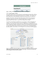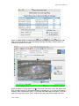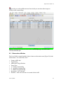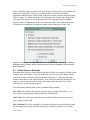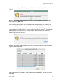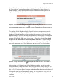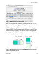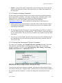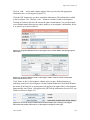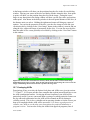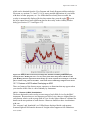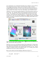
1
Spitzer Space Telescope
See Spot Run
Spot User’s Guide
Spitzer Planning Observations Tool 18
June 18, 2008
Issued by the
Spitzer Science Center
California Institute of Technology
Pasadena, California USA
http://ssc.spitzer.caltech.edu/
Spot User’s Guide v18
Table of Contents
1
2
3
Introduction............................................................................................................... 7
What is new in Spot?................................................................................................. 8
Minimum Recommended Hardware Configuration.................................................... 8
3.1
3.2
3.3
3.4
3.5
4
Operating System Configurations Supported ............................................................. 9
4.1
4.2
4.3
4.4
5
Windows Installation .............................................................................................................................10
Solaris or Linux Installation..................................................................................................................10
Mac Installation .....................................................................................................................................10
Spot Automatic Update .........................................................................................................................10
General Information ................................................................................................ 11
6.1
6.2
6.3
6.4
6.5
7
UNIX: Solaris 2.8+.................................................................................................................................9
Windows: NT, 2000, XP, Vista .............................................................................................................9
Linux: RedHat 8.0, 9.0; Fedora Core; Enterprise .................................................................................9
Mac: OS X................................................................................................................................................9
Installing and Starting Spot – Part of Spitzer Pride .................................................. 10
5.1
5.2
5.3
5.4
6
Sun Workstations: Sun Ultra 5 with 256 MB RAM..............................................................................8
Windows PC (2000, NT, XP): 512 MB RAM.......................................................................................8
Windows PC (Vista): 1 GB RAM ..........................................................................................................8
Linux PC: 256 MB RAM ........................................................................................................................8
Mac PC: OS 10.4, 512 MB RAM; OS 10.5, 1 GB RAM .....................................................................9
Client-Server Software Interactions .....................................................................................................11
On-line Help and Tool Tips ..................................................................................................................12
Time Estimates.......................................................................................................................................12
Maximum Duration of AORs ...............................................................................................................12
Troubleshooting .....................................................................................................................................13
Spot Menus ............................................................................................................. 13
7.1 File Menu ...............................................................................................................................................13
7.1.1 Open AORs and Targets [ctrl-O] ................................................................................................13
7.1.2 Save AORs and Targets [ctrl-S] ...................................................................................................14
7.1.3 Import Fixed Single Target List [ctrl-I] ......................................................................................16
7.1.4 Import Moving Single Target List [shift-ctrl-I]...........................................................................17
7.1.5 Save Target Background Estimates...............................................................................................17
7.1.6 Save Target Visibility Windows....................................................................................................17
7.1.7 Save Current Plotted Image as FITS file [ctrl-F] ........................................................................17
7.1.8 Save Current Plotted Image & Overlays to JPEG, GIF, BMP, PNG [ctrl-J] ............................17
7.1.9 View Program [ctrl-K] ..................................................................................................................18
7.1.10 Search Programs ...........................................................................................................................19
7.1.11 Check In Program [shift-ctrl-W] ................................................................................................19
7.1.12 Quit [ctrl-Q] .................................................................................................................................20
7.2 Edit Menu ...............................................................................................................................................20
7.2.1 Undo [ctrl-Z]...................................................................................................................................20
7.2.2 Delete Selected AORs [ctrl-X, delete] ..........................................................................................20
7.2.3 Modify Current AOR [ctrl-M].......................................................................................................20
7.2.4 Copy Selected AORs [ctrl-C] ........................................................................................................20
7.2.5 Delete All AORs.............................................................................................................................20
7.2.6 Delete All Targets...........................................................................................................................20
7.2.7 Enable All AORs [ctrl-E]..............................................................................................................21
7.2.8 Disable All AORs without G/F Constraints [ctrl-D]...................................................................21
7.2.9 Toggle ON Flag (AORs without G/F Constraints) [ctrl-W].......................................................21
7.3 Targets Menu .........................................................................................................................................21
7.3.1 New Target [ctrl-T] .......................................................................................................................21
7.3.2 Delete Selected Targets..................................................................................................................21
June 18, 2008
2
Spot User’s Guide v18
7.3.3 Modify Target .................................................................................................................................21
7.3.4 Target List [ctrl-L].........................................................................................................................21
7.3.5 Calculate Visibility Windows for All Targets ..............................................................................21
7.3.6 Calculate Background for All Targets ..........................................................................................22
7.4 Observation Menu..................................................................................................................................22
7.5 Tools Menu ............................................................................................................................................23
7.5.1 AOR Replication Tool ...................................................................................................................23
7.5.2 Target Replication Tool .................................................................................................................23
7.5.3 Group/Follow-on Constraints [ctrl-N] .........................................................................................23
7.5.4 Timing Constraints [shift-ctrl-N] .................................................................................................23
7.5.5 Proposal Submission Tool [shift-ctrl-P] ......................................................................................23
7.5.6 Show Current Resource Estimates [ctrl-A]..................................................................................23
7.5.7 Recompute All Estimates [shift-ctrl-A] .......................................................................................23
7.5.8 Compute Backgrounds from File ..................................................................................................24
7.5.9 Memory Monitor ............................................................................................................................24
7.6 Images Menu ..........................................................................................................................................24
7.6.1 ISSA and IRIS – IRAS Sky Survey Atlas ....................................................................................25
7.6.2 2MASS – Two Micron All Sky Survey ........................................................................................26
7.6.3 MSX – Midcourse Space Experiment...........................................................................................26
7.6.4 DSS – Digitized Sky Survey..........................................................................................................27
7.6.5 SkyView – SkyView image data ...................................................................................................27
7.6.6 NED – NASA/IPAC Extragalactic Database ...............................................................................29
7.6.7 ISO Image Archive.........................................................................................................................29
7.6.8 NVO Image.....................................................................................................................................29
7.6.9 FITS File .........................................................................................................................................30
7.6.10 FITS file from URL......................................................................................................................31
7.6.11 All Sky Images .............................................................................................................................32
7.6.12 Blank Image..................................................................................................................................33
7.7 Overlays Menu .......................................................................................................................................33
7.7.1 Catalog Overlay ..............................................................................................................................33
7.7.2 Crop .................................................................................................................................................37
7.7.3 Grid, a.k.a Coordinate Grid Overlay [ctrl-G] ..............................................................................37
7.7.4 Distance Tool [shift-ctrl-D] ..........................................................................................................37
7.7.5 Slice Tool ........................................................................................................................................38
7.7.6 Area Statistics Tool ........................................................................................................................38
7.7.7 Mark Object on Plot/User Created Catalog ..................................................................................38
7.7.8 Current Fixed Target ......................................................................................................................38
7.7.9 Add Moving Target ........................................................................................................................40
7.7.10 Image Overlays.............................................................................................................................40
7.7.11 Show All Known Moving Objects at a Date ..............................................................................40
7.7.12 Spitzer Focal Plane.......................................................................................................................40
7.7.13 Generic Focal Plane .....................................................................................................................41
7.7.14 AORs on Images [shift-ctrl-O] ...................................................................................................42
7.7.15 Read AOR Overlay Mapping File...............................................................................................43
7.7.16 Show Spitzer OPZ ........................................................................................................................44
7.7.17 Spitzer Bright Objects for AOR ..................................................................................................44
7.7.18 Show Depth of Coverage Maps on Current Image ....................................................................45
7.8 Options Menu.........................................................................................................................................47
7.8.1 User Automatic Spot Version Update...........................................................................................47
7.8.2 Sum Only Checked AORs .............................................................................................................47
7.8.3 Sort by Dec, then RA .....................................................................................................................47
7.8.4 Visualization: Spitzer Focal Plane Options ..................................................................................47
7.8.5 Visualization: Coordinate System Prefs........................................................................................47
7.8.6 Visualization: Readout Prefs .........................................................................................................47
7.8.7 Cache Prefs .....................................................................................................................................48
7.8.8 Network Proxy Setup .....................................................................................................................48
June 18, 2008
3
Spot User’s Guide v18
7.8.9 Use Large Control Icons ................................................................................................................48
7.8.10 Visualization: Show Mouse Help [shift-ctrl-M]........................................................................48
7.8.11 Visualization: Show Side Bar on Current Frame [shift-ctrl-B]................................................49
7.8.12 Visualization: Show Side Bar on All Frames [ctrl-B] ..............................................................49
7.9 Window Menu........................................................................................................................................49
7.10 Help Menu............................................................................................................................................49
7.10.1 Overview…...................................................................................................................................49
7.10.2 Tip Of The Day.............................................................................................................................49
7.10.3 AOR File Format Changes ..........................................................................................................49
7.10.4 AOT Field Descriptions ...............................................................................................................50
7.10.5 About….........................................................................................................................................50
7.11 Spot v18 Menu Command Summary (a.k.a. the Cheetah Sheet) .....................................................51
8
Spot Main Screen .................................................................................................... 54
8.1
8.2
8.3
9
Icons........................................................................................................................................................54
Observations Window ...........................................................................................................................56
Bottom Bar .............................................................................................................................................58
Entering An Astronomical Observation Request...................................................... 59
9.1 Start the Spot software...........................................................................................................................59
9.2 Enter Target Information.......................................................................................................................59
9.3 Fill Out an Astronomical Observation Template.................................................................................59
9.3.1 Unique AOR Label.........................................................................................................................59
9.3.2 Target Buttons ................................................................................................................................59
9.4 Enter Special ..........................................................................................................................................59
9.5 Obtain Resource Estimates....................................................................................................................60
9.6 Other AOT Buttons................................................................................................................................62
9.6.1 Source Flux Density .......................................................................................................................62
9.6.2 Sensitivity........................................................................................................................................62
9.6.3 Comments .......................................................................................................................................62
9.6.4 Special .............................................................................................................................................62
9.6.5 Vis. Window ...................................................................................................................................62
9.7 Save AORs .............................................................................................................................................63
10
The Target Entry Dialog........................................................................................ 64
10.1 Target Types ........................................................................................................................................65
10.1.1 Fixed Single ..................................................................................................................................65
10.1.2 Fixed Cluster-Offsets ...................................................................................................................66
10.1.3 Fixed Cluster-Positions ................................................................................................................67
10.1.4 Moving Single ..............................................................................................................................68
10.1.5 Moving Cluster .............................................................................................................................68
10.2 Inertial Target Coordinate Systems ....................................................................................................68
10.2.1 Coordinate Entry Formats............................................................................................................68
10.2.2 Coordinate Conversion ................................................................................................................70
10.2.3 Entering Targets at the Celestial Pole .........................................................................................70
10.3 Moving Target Entry ...........................................................................................................................70
10.3.1 Standard Ephemeris......................................................................................................................70
10.3.2 User Defined Ephemeris ..............................................................................................................71
10.3.3 Shadow Observations...................................................................................................................72
10.4 Target Name Resolution......................................................................................................................74
10.5 Bright Moving Object Avoidance ......................................................................................................74
10.6 Target List ............................................................................................................................................75
10.7 Visibility Windows..............................................................................................................................76
10.7.1 Visibility Windows for Inertial Targets ......................................................................................76
10.7.2 Moving Object Visibility Information ........................................................................................76
10.7.3 Spitzer Planning with Horizons...................................................................................................76
10.8 Position Angle: Focal Plane, IRS Slits, MIPS Scan & SED Slit.....................................................77
10.9 Estimating the Sky Background .........................................................................................................79
June 18, 2008
4
Spot User’s Guide v18
10.9.1
10.9.2
10.9.3
10.9.4
11
IRAS Sky Maps ............................................................................................................................79
Spot Background Estimate...........................................................................................................80
Batch Mode Background Estimates ............................................................................................80
Compute Backgrounds from File ................................................................................................80
Astronomical Observation Templates .................................................................... 83
11.1 IRAC Mapping.....................................................................................................................................83
11.1.1 Subarray Mode .............................................................................................................................85
11.1.2 Stellar Mode..................................................................................................................................85
11.1.3 Mapping versus Dithering............................................................................................................87
11.1.4 Map Rows and Columns ..............................................................................................................88
11.1.5 Post-Cryo AOT.............................................................................................................................89
11.2 IRS Staring Mode ................................................................................................................................89
11.2.1 Standard Staring ...........................................................................................................................90
11.2.2 Peak-up Targets ............................................................................................................................90
11.2.3 Peak-up Only ................................................................................................................................96
11.2.4 Peak-up Target Flux Limits .........................................................................................................96
11.2.5 Moving Target Peak-up ...............................................................................................................97
11.3 IRS Spectral Mapping .........................................................................................................................99
11.4 IRS High-Resolution Modules and Sky Background Observations...............................................100
11.5 IRS Peak-Up Imaging........................................................................................................................104
11.6 MIPS Scan Map .................................................................................................................................104
11.6.1 In-Scan Versus Cross-Scan Directions .....................................................................................104
11.6.2 160 µm Data Required Checkbox ............................................................................................104
11.6.3 MIPS Scan 160 µm data warnings ...........................................................................................105
11.7 MIPS Photometry/Super Resolution ................................................................................................105
11.7.1 Raster Map: Rows vs. Columns ...............................................................................................106
11.7.2 Enhanced Photometry Mode for 160 µm..................................................................................107
11.8 MIPS Spectral Energy Distribution ..................................................................................................107
11.9 MIPS Total Power Mode...................................................................................................................108
12
Tools for Replicating AORs ................................................................................ 109
12.1
12.2
13
AOR Replication Tool.......................................................................................................................109
Target Replication Tool.....................................................................................................................109
Constraints Editing .............................................................................................. 111
13.1 Description .........................................................................................................................................111
13.2 Timing Constraints ............................................................................................................................111
13.3 Grouping/Follow-on Constraints ......................................................................................................112
13.3.1 Description..................................................................................................................................112
13.3.2 Caveats for Grouping Constraints .............................................................................................114
13.3.3 Creating New Grouping and Follow-on Constraints................................................................114
13.3.4 Linking AORs to a Grouping Constraint ..................................................................................115
13.3.5 Creating a Follow-on Constraint ...............................................................................................117
13.3.6 Creating a Shadow Constraint ...................................................................................................120
14
Proposal Submission Tool ................................................................................... 121
14.1 Proposal Submission Tool Main Window .......................................................................................121
14.1.1 File Menu ....................................................................................................................................122
14.1.2 Submit Menu ..............................................................................................................................123
14.1.3 Help .............................................................................................................................................124
14.2 Add Principal Investigator Information ...........................................................................................124
14.3 Add Contact Information ..................................................................................................................124
14.4 Add Co-Investigators.........................................................................................................................125
14.5 Add Proposal Abstract.......................................................................................................................127
14.6 Add Scientific Justification File .......................................................................................................127
14.7 Add Science Category Information ..................................................................................................128
14.8 Add any Extra Text............................................................................................................................129
June 18, 2008
5
Spot User’s Guide v18
14.9 Add Joint Observatories ....................................................................................................................129
14.10 Hours Requested in the Proposal (non-Archive and Theory proposals only)..............................130
14.11 Dollars Requested – Archive and Theory Proposals Only............................................................130
14.12 The Final Stretch – Submitting the Proposal .................................................................................130
14.12.1 The Prologue.............................................................................................................................130
14.12.2 Submitting the Proposal ...........................................................................................................130
14.12.3 Updating an Existing Proposal ................................................................................................133
14.13 Submitting a Spitzer Observing Proposal – Review .....................................................................134
15
Fixed Target and AOR Visualization ................................................................... 136
15.1 Displaying and Manipulating Images...............................................................................................136
15.1.1 Image Control .............................................................................................................................136
15.1.2 Image Window Control..............................................................................................................137
15.1.3 Cursor Readout ...........................................................................................................................137
15.1.4 Layer Control..............................................................................................................................137
15.1.5 Three-Color Image Display .......................................................................................................137
15.1.6 Cropping Images ........................................................................................................................140
15.1.7 Measuring Area Statistics ..........................................................................................................140
15.2 Current Fixed Target Overlay ...........................................................................................................143
15.3 Overlaying a Coordinate Grid...........................................................................................................143
15.4 Overlaying a Catalog .........................................................................................................................143
15.5 Overlaying an Image .........................................................................................................................146
15.6 Using the Slice Tool ..........................................................................................................................146
15.7 Overlaying AORs ..............................................................................................................................147
15.7.1 Features of AOTs when Overlaying an AOR...........................................................................148
15.7.2 IRAC Mapping AOR .................................................................................................................149
15.7.3 IRS Staring AOR........................................................................................................................152
15.7.4 Overlaying Multiple AORs........................................................................................................153
15.7.5 IRS Spectral Mapping AOR ......................................................................................................154
15.7.6 IRS Peakup Imaging AOR.........................................................................................................155
15.7.7 MIPS PH/SR AOR .....................................................................................................................157
15.7.8 MIPS Scan AOR.........................................................................................................................158
15.7.9 MIPS SED AOR.........................................................................................................................159
15.7.10 MIPS Total Power AOR ..........................................................................................................160
15.8 List of the Spitzer Fields-of-View ....................................................................................................161
16
Moving Target Visualization ............................................................................... 164
16.1 Overview ............................................................................................................................................164
16.2 Getting Started ...................................................................................................................................164
16.2.1 Selecting a Background Sky Image ..........................................................................................164
16.2.2 Selecting an Observation Date ..................................................................................................164
16.3 Getting Fancy .....................................................................................................................................166
16.3.1 Highlighting Points and Displaying Date Markings on a Moving Target Trajectory............167
16.3.2 Adding Your Own Marks/Labels to a Trajectory or Image.....................................................169
16.3.3 The Distance Tool ......................................................................................................................169
16.3.4 Displaying the Spitzer Focal Plane ...........................................................................................170
16.3.5 Displaying the Spitzer Diffraction Spikes ................................................................................171
16.4 Displaying Moving Target AORs.....................................................................................................171
16.4.1 Displaying an AOR ....................................................................................................................172
16.4.2 An Illustrative Example .............................................................................................................173
16.5 Add Moving Target ...........................................................................................................................174
17
18
Sample Spot Target File ...................................................................................... 177
Sample AOR File ................................................................................................ 180
June 18, 2008
6
Spot User’s Guide v18
1 Introduction
Welcome to Spot – the tool for planning Spitzer observations and submitting proposals.
The Spot software is available to download from the Proposal Kit page at the Spitzer
Science Center SSC web site (http://ssc.spitzer.caltech.edu/propkit/spot/).
The process of planning a Spitzer observation with Spot consists of entering targets that
are individually linked to a desired Spitzer observing mode via an Astronomical
Observation Template (AOT). The instrument parameters that completely specify the
observation are entered via the AOT. The complete target + instrument information
results in an Astronomical Observation Request (AOR), the primary unit of Spitzer
observing. Spot allows you to determine how much time will be required to execute the
observation by obtaining an estimate from the AIRE (AOR Interpreter and Resource
Estimator) server software at the SSC. This is the amount of time you must request for
this AOR in your observing proposal.
This User’s Guide provides information about how the Spot software works. The Release
Notes that are packaged with the software provide additional information about computer
platforms supported for this version, performance issues, and a list of known bugs. A list
of bugs/issues is updated regularly on the Proposal Kit web page
(http://ssc.spitzer.caltech.edu/propkit/).
To make using Spot and planning your Spitzer observations easier, we recommend that
you:
1. Read the relevant sections of the Spitzer Observer’s Manual (available on the SSC
website) to decide how best to implement your observations.
2. Read the Release Notes that are packaged with the software (or download them from
the web page). Some, but not all, of that information is repeated here.
3. Check the Proposal Kit web page for additional information in helping you plan your
observations. Check the known bugs/issues list on the web page as well.
4. Save your AORs often. Spot does not save your work to disk automatically. Given
the variety of operating systems we support, we cannot guarantee that it won’t crash.
Saving your work often will make these events, though rare, much less painful.
Please email us at the Spitzer Help Desk ([email protected]) with any questions
or comments.
June 18, 2008
7
Spot User’s Guide v18
2 What is new in Spot?
Several items have changed in this version of Spot. In addition, we have added a number
of new features. We have attempted to encapsulate in the list below the most obvious
changes that affect users the most:
•
•
•
•
•
•
•
•
•
•
Provide Exposures table for IRAC AOTs.
Allow for switching between array and celestial coordinates for Fixed Cluster targets.
Background calculation output format modified.
Visualization: Load FITS images from a URL.
Visualization: Load images from NVO Simple Image Access Protocol (SIAP) sites.
Visualization: Slice Tool now handles image overlay layers.
Visualization: Allow for creation of blank image for overlays.
Visualization: Removed 10° limit on Depth-of-Coverage overlays for MIPS Scan
AORs.
Visualization: Allow for Depth-of-Coverage overlays for IRAC Post-Cryo Mapping
AORs.
Various other improvements and bug fixes.
3 Minimum Recommended Hardware Configuration
Spot is written in the JAVA language and therefore requires lots of memory and a fast
processor in your computer. If you run Spot on a system with less memory or processor
power than our minimum recommended configuration, the software may work, but it is
likely to be slow, and you will probably see window redraw/refresh problems. While we
suggest minimum hardware configurations, we recommend that users have more RAM
(512 MB or above) and a fast processor if you plan on intensive use of the visualization
features within Spot. The minimum recommended hardware configurations are:
3.1 Sun Workstations: Sun Ultra 5 with 256 MB RAM
If you are not using the visualization features in Spot, then it may run acceptably on an
Ultra 1 with 256 MB of RAM.
3.2
Windows PC (2000, NT, XP): 512 MB RAM
3.3
Windows PC (Vista): 1 GB RAM
3.4 Linux PC: 256 MB RAM
We have done limited testing on Linux systems running with a Pentium 2 processor at
266 MHz and 256 MB of RAM, as well as with a Pentium 3 processor and 256 MB of
RAM.
June 18, 2008
8
Spot User’s Guide v18
3.5 Mac PC: OS 10.4, 512 MB RAM; OS 10.5, 1 GB RAM
We have tested Spot on a G4 with 512 MB RAM under OS 10.4, and it runs acceptably.
However, we recommend 1 GB RAM for OS 10.5 (Leopard).
4 Operating System Configurations Supported
Please read the Release Notes (packaged with the software or available on the web page)
for more details on operating system issues, particularly with respect to window
managers. The majority of the testing for this version of Spot has been done under Solaris
2.8 and Windows XP, Linux, and Mac OSX. We do not anticipate major problems with
other flavors of Windows. Except for Mac, the versions of Spot in this release come with
JAVA 1.5.
4.1 UNIX: Solaris 2.8+
The software has been tested on Solaris 2.8 and 2.10.
4.2 Windows: NT, 2000, XP, Vista
The functionality of the software has been tested using Windows XP. Minimal testing has
been completed using other versions of Windows, but we do not anticipate problems.
Due to the security measures for Windows Vista, you will need system administration
privileges for software installation. To allow auto-update under Windows Vista, use the
right mouse button when clicking on the Spot icon, and select “Run as Administrator.”
You can click on the icon and run Spot normally thereafter.
4.3 Linux: RedHat 8.0, 9.0; Fedora Core; Enterprise
Spot on Linux runs acceptably on RedHat 8.0, 9.0. We tested each distribution “straight
out of the box”. We ran the GNOME windowing environment. We know that Spot does
NOT run properly with the fvwm2 window manager (all JAVA Swing programs seemed
to hang) or KDE. Spot did seem to run OK with the older fvwm window manager, but
our testing was only cursory. Spot also appears to run well under Fedora Core, although
we have not yet fully tested Fedora Core 4 or 5. Undoubtedly, there will be various Linux
OS under which Spot will not run successfully. For example, we are not supporting
Spitzer Pride for 64-bit Linux machines. You will need to install the ‘generic’ package
and download your own Java; see the Installation webpage.
4.4 Mac: OS X
Spot requires JAVA 1.5, so Mac OS 10.4 or 10.5 are required. (Note: Spot will not run
under Mac OS 10.3.) Apple offers JAVA 1.5 (JAVA 2 Standard Edition [J2SE] 5.0) as a
software update. By now, nearly all Mac OS 10.4 or 10.5 systems should be running
JAVA 1.5, unless you have not allowed software updates to run over a year or so. You
may need system administration privileges for software installation.
June 18, 2008
9
Spot User’s Guide v18
5 Installing and Starting Spot – Part of Spitzer Pride
With this release we continue the tradition of Spitzer Pride – Spot V18 and Leopard V9.
Spot and Leopard share many of the same JAVA files and so are packaged together as
Spitzer Pride. Spot/Leopard should be installed on the computer where you want to run it.
The start-up script is not configured to allow it to run on an X-terminal. You can run
them across a Sparc network if it is installed on a disk that is nfs mounted across the
network. We can run Spot and Leopard in this fashion at the SSC. The first step is to
download the software from the SSC Proposal Kit web page onto your hard disk
(http://ssc.spitzer.caltech.edu/propkit/spot/).
5.1 Windows Installation
After downloading the software, double-click on the Spitzer-pride18-windows.exe file to
install Spot. Click on the Spot icon to start the program.
5.2
Solaris or Linux Installation
1. Go to the directory where you installed the Spitzer-pride18-solaris.sh or
Spitzer-pride18-linux.sh file. You must have write permission in this directory
and should have at least 200 MB of free disk space.
2. At the UNIX/Linux prompt, type chmod +x Spitzer-pride18-solaris.sh (or
Spitzer-pride18-linux.sh) to make the file executable.
3. Type ./Spitzer-pride18-solaris.sh (or Spitzer-pride18-linux.sh) to run the
installation script.
4. When the script asks you for the directory name where you want to install Spot,
be sure to type the full directory path, e.g., /scr/user/my_pride. Make sure the
directories exist before you try to install it there. If you are in the directory
/scr/user/ and just type my_pride, it will tell you that the directory name must
start with a slash.
5. If desired, add this directory to your $PATH: setenv PATH ($path
/scr/user/my_pride)
6. Type the name of the program (spot or leopard) to launch it.
5.3 Mac Installation
Click on the link for the software package, offered as a disk image (.dmg) file. Drag the
Spitzer-pride folder icon from the pop-up window onto your local disk into whichever
directory you want to install the software. For instance, you may wish this to be the
Applications folder. Double-click on the program to install it. Click on the Spot
executable to start Spot.
5.4 Spot Automatic Update
The automatic update feature from the Options menu will allow the client side of Spot to
update itself if it detects that a newer version is available at the SSC. Spot will access the
updated files at the SSC via the Internet and will automatically install them on your
computer. Auto-update is the default setting when you first install Spitzer Pride. If you
turn this feature off, or decline an auto-update at any time, Spot will remember that you
June 18, 2008
10
Spot User’s Guide v18
have turned it off. We strongly encourage users to leave auto-update turned on and to
accept auto-updates when they occur. Note, to allow auto-update under Windows Vista,
use the right mouse button when clicking on the Spot icon, and select “Run as
Administrator.” You can click on the icon and run Spot normally thereafter.
6 General Information
6.1 Client-Server Software Interactions
The Spot software that you download onto your computer acts as the ‘client’ and requests
information over the network from the ‘server’ software located at the Spitzer Science
Center (SSC). The main server that provides observing time estimates for Spot is called
AIRE, i.e., the AOR Interpreter and Resource Estimator. (An AOR is an Astronomical
Observation Request.)
Entry of targets and Astronomical Observation Template (AOT) parameters are selfcontained within Spot. An Internet connection to contact the servers is required to
calculate observing time estimates, obtain visibility windows, obtain background
estimates, and download astronomical images and catalogs.
When the servers are accessible by Spot, the net-up symbol (Figure 1) will appear at the
bottom of the main Spot window.
Figure 1: The net-up symbol means Spot can access the SSC servers. The net must be up to calculate
observing time estimates, obtain visibility windows, obtain background estimates, or download
images or catalogs.
If your computer is not connected to the Internet or if our servers are temporarily down,
the net-down symbol (Figure 2) will appear at the bottom of the main Spot window.
Figure 2: The net-down symbol means Spot cannot access the SSC servers. You may still enter
target and AOT information when the net is down but you cannot calculate observing time estimates,
obtain visibility windows, obtain background estimates, or download images or catalogs.
Check the Release Notes if you are using a Windows PC and never see the net-up
symbol. This has been noted in two instances, and the fix is described in the Release
Notes. If you see the net-down symbol and believe that Spot should be connected to the
servers, please send email to the Helpdesk at [email protected]. We do not yet
provide 24-hour support for the SSC servers. We have computer support available
weekdays during business hours, so if our servers go down late Friday evening, they may
not come back up until Monday morning.
June 18, 2008
11
Spot User’s Guide v18
6.2 On-line Help and Tool Tips
In addition to the Release Notes, this User’s Guide, and the Spitzer Observer’s Manual,
on-line help for Spot is available from the help menu on the main Spot screen. There are
also help buttons throughout the program that connect directly to applicable help files.
On-line help is also available in the form of ‘tool tips’, one-sentence messages that
appear whenever the cursor is placed over a field or button for longer than 3 seconds.
Tool tips are used to define acronyms, expand abbreviations, and provide data entry
instructions. For example, placing the cursor over the new target (“bulls-eye”) button in
the icon bar displays the tool tip that says, “Create a new target of any type” (Figure 3).
Figure 3: A ‘tool tip’ is displayed by placing the cursor over the “bulls-eye” icon. This icon brings up
the dialog for creating a new target.
6.3 Time Estimates
In calculating the time estimates, we have used all the information available to date about
the instruments and flight software performance. We expect that these estimates are good
to at least 10% of the total ‘AOR duration’ or ‘wall-clock time’. Spot reports the
following when you request an observing time estimate:
1. AOR Duration: This is the ‘wall-clock’ time or total time required to execute
the observation, including time on source, internal calibrations, slewing,
settling, command execution, and the fixed slew overhead applied to each
AOR. This is the time you must request in your proposal for this observation.
2. Slew Time: The time spent on slews internal to the AOR.
3. Settle Time: The time required for the telescope to settle after slews internal
to the AOR.
4. Slew Overhead: A 215 second overhead applied to all AORs to account for
the initial slew to source and other observatory overheads.
5. Moving Target Overhead: A 300 second special overhead is included in the
slew overhead for moving targets.
6. Integration Time(s): Estimated on-source integration time(s) in seconds.
Spot v18 returns observing time estimates from AIRE for all of the AOTs.
6.4 Maximum Duration of AORs
The duration limits for all AORs are 3 hours for MIPS and 8 hours for IRAC and IRS. If
the estimated duration (not including the slew overhead) of your AOR is longer than
these times, the software will return a message telling you to make the observation
shorter. In general, AORs longer than about 3 hours may be more difficult to schedule.
If your science results in AORs substantially longer than this, you can create separate
June 18, 2008
12
Spot User’s Guide v18
shorter duration AORs and use a sequencing constraint (section 13.3), so that they are
executed serially.
6.5 Troubleshooting
The current list of known bugs and issues is updated regularly and kept on the Proposal
Kit web page from which you downloaded this software. If you think you have found a
bug, before reporting it please check the bugs list and the troubleshooting section of the
Release Notes to discover if it is a ‘feature’ we already know about. Also check the
appropriate section of this Guide and the Spitzer Observer’s Manual to understand what
the software is doing.
If you find a real bug, then please do let us know about it.
1. Email a description of the problem to the Helpdesk at [email protected].
2. Include the hardware configuration you are using (e.g., SunBlade 100, 512 MB).
3. Please attach the Spot log file, created in the default directory when you install the
software. Each time you run Spot, it creates a file called ‘spot_DATE_TIME.log.’ The
default directories are:
Solaris/Linux/Mac
Windows ME
Windows NT/2000/XP
Windows Vista
/home/<username>/.spot
c:\spot
c:\Documents and Settings\{username}\Application Data\Spot
c:\Users\[username]\AppData\Roaming\spot
The text showing in any error windows that pop up in Spot should show up in the logfile
as well.
7 Spot Menus
Spot has ten menus that provide the tools needed to create your AORs. Section 7.11 gives
a single page summary of all the Spot menu items. The menus provide the following
functions.
7.1 File Menu
File I/O is handled from this menu.
7.1.1 Open AORs and Targets [ctrl-O]
This function opens a dialog to select a file of targets or AORs that has previously been
written out with Spot. AOR and target files are plain ASCII text files created by Spot
with the formatting required by the software. Spot expects AOR files to have the suffix
‘.aor’ and Spot target files to have the suffix ‘.tgt’. Sample files illustrating the format
required for targets and AORs are included in sections 17 and 18, respectively.
The ‘Read AORs and Targets’ dialog is shown in Figure 4. You can browse directories
and select a target or AOR file from the list or type in the name. (Note that the directory
structure in the dialog is now compatible with the default Mac OSX directory structure.)
June 18, 2008
13
Spot User’s Guide v18
At the right side (or bottom) of the dialog, you can select the method Spot should use for
handling duplicate AORs, i.e., if an AOR file you are reading in contains an AOR with
the same ‘Unique AOR Label’ as one already loaded in Spot. The default is for Spot to
read in the duplicates and append ‘copy’ to the labels, so that they remain unique. The
name of the last AOR file read into Spot will appear in the lower left corner of the main
Spot window. You can also select to discard duplicate AORs, as well as overwrite AORs
already in Spot with AORs read in from local disk.
Figure 4: The ‘Open AORs and Targets’ dialog.
If you are a Linux user, and are trying to read your saved AORs in the default directory
of /home/<username>/.spot you may need to enter the full pathname in the filename field.
7.1.2 Save AORs and Targets [ctrl-S]
This function opens a dialog to allow you to write out either your targets (in Spot format,
see section 17) or your AORs to text files. Spot writes out AOR files with the suffix
‘.aor’ and Spot target files have the suffix ‘.tgt’. These are plain ASCII text files created
by Spot with the required formatting. Sample files illustrating the format required for
targets and AORs are included in sections 17 and 18, respectively.
When writing out AOR files, you can either write out all of your AORs or a subset of
files for which you have set the ‘ON’ flag. It is important that you save your AORs
before exiting Spot, otherwise your work will be lost. Spot does not save AORs or
targets to disk automatically. If you do not select a directory in which to save your files,
the default directory is:
Solaris/Linux/Mac
Windows 95,98,ME
Windows NT/2000/XP
Windows Vista
June 18, 2008
/home/<username>/.spot
c:\spot
c:\Documents and Settings\{username}\Application Data\Spot
c:\Users\[username]\AppData\Roaming\spot
14
Spot User’s Guide v18
When you select ‘Save AORs and Targets’, the dialog shown in Figure 5 opens. The
default function for this dialog is to save AORs to a file. The default file Spot creates is
named ‘newfile.aor’. (If you include the ‘.aor’ suffix in the File name, Spot will still
create the filename ‘newfile.aor’). If you read in a file of AORs and save them to a new
file name, the file name in the lower left corner of the Spot window will not change. It
continues to show the last AOR file that was read into Spot. A sample AOR file is shown
in section 18.
Figure 5: The ‘Save AORs and Targets’ dialog is shown with the ‘Save AORs’ radio button selected.
In this example we are writing the AORs to a file named ‘m31.aor.’ If instead of saving a file of
AORs you want to save just targets to a file, select the ‘Save Target list’ radio button near the bottom
of the window. The dialog then changes to the form shown in Figure 6. Spot is now ready to save a
file of the currently entered targets called ‘newfile.tgt’.
Figure 6: The ‘Save AORs and Targets’ dialog is shown after selecting the ‘Save Target list’ radio
button. Spot will save the targets you have entered to a file using the format shown in section 17.
June 18, 2008
15
Spot User’s Guide v18
7.1.3 Import Fixed Single Target List [ctrl-I]
Spot can read in single target/line lists for inertial targets. This function has not yet been
implemented for fixed or moving cluster targets. A sample file is shown below, and the
required format of the file is described. Spot will resolve the name from the target list:
The keyword, “NAME-RESOLVER,” can be input at the top of the list, with values
either “ned” or “simbad.” If the target list with this keyword included contains a line
consisting only of a target name, the name resolver is contacted via the Internet to
retrieve the positional information. Spot must be connected to the Internet for this feature
to function.
An example target list looks like the following:
COORD_SYSTEM: Equatorial
EQUINOX: B1950
NAME-RESOLVER: ned
# Name
RA/LON
"NGC 001" 12h34m23.45s
NGC2222
23.56d
NGC4444
"12 34 12.23"
NGC4321
•
•
•
•
•
•
•
# Equatorial, Galactic, or Ecliptic
# B1950, J2000, or blank for Galactic
# Name resolution by either NED or SIMBAD
DEC/LAT
PM-RA PM-DEC EPOCH
34d23m56.2s 2.3
3.4
1950.3
34.456d
2.3
3.4
1950.3
"34 23 45.45" 2.3
3.4
1950.3
The first two keywords give the coordinate system and equinox for all the positions in
this list; these keywords are optional.
The list columns are separated by spaces. If there are spaces in the values for a
column, double quotes are needed surrounding the value. This is particularly true for
name resolving.
Any lines starting with the pound sign (#) will be treated as comments.
Proper motion for RA and DEC, in arcseconds, are not required, may only be entered
for Equatorial coordinates, and must always be supplied in RA and Dec pairs.
If the value for the fourth column is larger than 1900.0, it is interpreted as the epoch.
If it is smaller than 1900.0 it is assumed to be a proper motion, as discussed above.
The epoch field need only be entered for equinox B1950 coordinates.
You need to make separate lists/files for Equatorial J2000, Equatorial B1950,
Galactic, Ecliptic J2000, and Ecliptic B1950 coordinates, because the first two
keywords define the coordinate system for the entire file. These can then be read into
Spot one file at a time.
If only a name is listed in the first field, and a name resolver is specified (in the
example above, “ned”), the resolver will be contacted for positional information.
NED has a more forgiving name resolver, so a name string without spaces, e.g.,
“ NGC4321,” can be resolved. However, with SIMBAD, if a target name has a space,
don’t remove that space; instead, place the whole name string within double quotes for
the resolver to work.
You can create targets in the format required by Spot with a text editor and then read in
these files. Samples of all types of targets, in the proper format, are given in section 17.
June 18, 2008
16
Spot User’s Guide v18
7.1.4 Import Moving Single Target List [shift-ctrl-I]
Spot can read in lists of single moving targets. The format for the input file must follow
these rules:
Comments must start with # or !.
Each line should have at most 2 elements. The first element is the NAIF Name and
the second is the NAIF ID if both elements are present.
• If only one element is provided, it is assumed to be the NAIF ID if it is all numbers
(put it in double quotes, if it is a name). If the one element has characters other than
numbers, it is assumed to be the name.
• If there are spaces in the name, put the entire name inside double quotes.
• The NAIF ID should NOT be in quotes.
If only one element is on the input line, Spot will attempt to resolve the missing Name or
ID. Spot will issue a warning message if a given name does not resolve a NAIF ID (and
no entry for the object will appear in the target list). If both Name and ID are provided,
both will be used as they appear on the input line.
•
•
An example moving single target list looks like the following:
“my targ name” 12345678
Mars_barycenter 4
Dione 2000106
604
2000159
Jupiter
7.1.5 Save Target Background Estimates
This menu item is only active if you have calculated background estimates for targets in
your target list (see sections 10.9.2 and 10.9.3). If you select it, you can write the current
background estimates in memory to a text file. Spot cannot read this file back in.
7.1.6 Save Target Visibility Windows
The menu item is only active if you have calculated visibility windows for targets in your
target list. If you select it you can write the current visibility windows in memory to a text
file. Spot cannot read this file back in.
7.1.7 Save Current Plotted Image as FITS file [ctrl-F]
If you are currently displaying an image in Spot selected from the Images menu, this will
save the image as a FITS file. It does not save any overlays, just the image.
7.1.8 Save Current Plotted Image & Overlays to JPEG, GIF, BMP, PNG [ctrl-J]
If you are currently displaying an image in Spot selected from the Images menu, this will
save the image, along with any overlays, as a GIF, JPEG, BMP (bitmap), or PNG format
file.
June 18, 2008
17
Spot User’s Guide v18
Figure 7: Dialog to enter a program ID number or name to View Program.
7.1.9 View Program [ctrl-K]
This feature allows you to view the abstract for and download into Spot all the AORs in
an approved Spitzer observing program directly from our database. You can then save
these AORs on your local disk and/or modify the most up-to-date set of AORs for a
program. You must be connected to the Internet and see the Net Up icon in Spot to
download a Program from the SSC. Program identification is by program name or
program identification number, entered in the dialog shown in Figure 7.
If you have just submitted a modification to your program via Check In Program (see
section 7.1.11), you will not be able to use View Program to ‘see’ the modification
immediately after submission. Programs that are Checked In for modification are loaded
into a ‘modification’ database and will be verified by the SSC before being transferred to
our Operations Database (this will likely take more than one day). When the Database
has been updated, you can then use View Program to see your newly modified program.
Figure 8: Dialog to search the SSC databases for AORs in approved programs with target positions
within the user-specified search radius around the current target. You can also select the AOT(s)
and wavelength(s) returned from these programs.
June 18, 2008
18
Spot User’s Guide v18
7.1.10 Search Programs
Selecting “Search Programs” will bring up a dialog, such as the one shown in Figure 8.
For any target in your list of targets, Spot will contact the databases at the SSC and search
for all AORs from approved programs with target positions within the user-specified
search radius. Units for the search radius can be in arcseconds, arcminutes, or degrees,
specified using the pulldown in the dialog. The minimum search radius is 1′. For moving
targets, Spot will search for all AORs corresponding to the target’s NAIF ID. You can
also select the AOT(s) and wavelength(s) you wish returned from the search. In effect, it
is now possible within Spot to search the Spitzer Reserved Observations Catalog (see
http://ssc.spitzer.caltech.edu/roc/), although we strongly recommend that you use
Leopard for this purpose instead. You must be connected to the Internet to search
programs. This works for both inertial and moving targets.
The results of the example search are shown in Figure 9. The AORs appear in the main
Observations window. The target information corresponding to the AORs returned by
the search are inserted into the current list of targets.
Figure 9: Results of the example search shown in Figure 8. The AORs found in the search appear in
the Observations window.
7.1.11 Check In Program [shift-ctrl-W]
Using the dialog shown in Figure 10, you can submit modifications to your Spitzer
observing programs to the SSC. You will need to have your complete program, including
any revised AORs loaded into Spot, as well as your program name and password (see
14.12.2; these are not your Leopard username and password!). You can use the View
Program feature (Section 7.1.9) to download your program as it currently exists in our
June 18, 2008
19
Spot User’s Guide v18
database, or import a trusted version of the program AORs from local disk, before
modifying the program. Any modification to a program must be approved by the SSC, so
please refer to the SSC Science User Support web pages on how to submit modifications
to your approved observing programs (http://ssc.spitzer.caltech.edu/ost/).
7.1.12 Quit [ctrl-Q]
Please be sure and save your AORs and/or targets before you select Quit, as Spot does
not do this automatically. If you have modified AORs that have not been saved to a file,
however, Spot will prompt you to save them when you attempt to quit the program.
Figure 10: The Check In Program dialog. You will need the program user name and password, as
well as having all modified AORs loaded into Spot, before resubmitting the program to the SSC. You
must be connected to the Internet in order to check-in programs.
7.2
Edit Menu
7.2.1 Undo [ctrl-Z]
This reverses the last action.
7.2.2 Delete Selected AORs [ctrl-X, delete]
Delete the selected AORs in the Observations table. If the selected AORs are
constrained, the constraints will be deleted as well.
7.2.3 Modify Current AOR [ctrl-M]
Open the AOT template for the AOR that is currently selected.
7.2.4 Copy Selected AORs [ctrl-C]
This makes duplicate entries of the selected AORs. The unique AOR labels are
automatically edited with the addition of ‘copy’ to remain unique.
7.2.5 Delete All AORs
This will clear ALL of the AORs in the AOR table from Spot. This action is NOT
reversible, so be sure you have saved any work you need to keep before you clear Spot.
7.2.6 Delete All Targets
This will clear ALL of the targets from the target list in Spot. This action is NOT
reversible, so be sure you have saved any work you need to keep before you clear Spot.
June 18, 2008
20
Spot User’s Guide v18
This does nothing to the target information in the AORs in the AOR table. It only clears
the target list in Spot’s memory.
7.2.7 Enable All AORs [ctrl-E]
This function turns the flag ON for all AORs currently in Spot. This function is most
likely to be used if you are planning to write out a subset of your AORs to a file or are
recalculating resource estimates for a subset.
7.2.8 Disable All AORs without G/F Constraints [ctrl-D]
This turns the flag OFF for all AORs that are not part of a Grouping or Follow-on
constraint (see section 13.3).
7.2.9 Toggle ON Flag (AORs without G/F Constraints) [ctrl-W]
For all AORs that are not part of a Grouping or Follow-on constraint (see section 13.3),
this turns the flag from OFF to ON, or ON to OFF. Once you have added Group/Followon constraints, Spot won’t let you turn theseAORs OFF. This prevents you from saving a
set of AORs and their associated constraints with ‘missing’ AORs because you
unintentionally turned one or more of the AORs OFF. All the AORs within each
constraint must be in the AOR file; otherwise, the constraint is not valid.
7.3 Targets Menu
The functions in the Targets menu are the following. Please refer to section 10.
7.3.1 New Target [ctrl-T]
Enter a new target from the target entry window.
7.3.2 Delete Selected Targets
Delete the currently selected targets. The name of the current target is displayed at the
bottom of the main screen.
7.3.3 Modify Target
Open a target entry dialog with the current target entered.
7.3.4 Target List [ctrl-L]
This opens a dialog showing a summary list of the targets currently loaded. Clicking on
an entry makes this target the 'current' target. The name will appear at the bottom of the
main Spot window. In addition, from this dialog window you can show the background
estimates and visibility windows for the list of targets. You can save them to disk by
selecting the appropriate option under the File menu. As you enter targets into Spot, the
target list appears at the bottom of the Targets pull-down menu. By selecting any of the
targets shown in the menu, you move that target to the top of the list.
7.3.5 Calculate Visibility Windows for All Targets
See section 10.7.1.
June 18, 2008
21
Spot User’s Guide v18
7.3.6 Calculate Background for All Targets
See section 10.9.3.
A VERY IMPORTANT NOTE: The targets in the Target List and the AORs are not
linked. If you change the coordinates in a target that you have already entered into an
AOR, they are NOT updated in that AOR, unless you modify the target from within the
AOT dialog.
To change the coordinates for a target already included in an AOR, load the AOR file
into Spot, double-click on the AOR to open it up, and then select the Modify Target
button within the AOR to correct/modify the coordinates.
7.4 Observation Menu
The selection of the desired AOT parameters is made from the Observation menu. The
Spitzer Observer’s Manual is your primary reference for information about using the
Spitzer instruments and selecting the appropriate AOT parameters. Additional
comments about the AOTs are provided in sections 9 and 11 of this Guide.
There are nine Spitzer AOTs fully implemented in Spot. Five of the AOTs were
commissioned within the first three months after launch; these are:
•
•
•
•
•
IRS Staring Mode
IRS Spectral Mapping
IRAC Mapping
MIPS Scan Map
MIPS Photometry/Super Resolution
A sixth AOT was available to Cycle-1 programs, but not commissioned until 6 months
after launch; this is:
•
MIPS Spectral Energy Distribution
Two additional AOTs became available to Cycle-2 observers; these are:
•
•
MIPS Total Power mode
IRS Peak-Up Imaging
For Cycle-3 the IRAC Mapping AOR was modified to include Stellar Mode (see section
11.1.2).
The MIPS Photometry/Super Resolution AOT has been modified to include an
“Enhanced” photometry mode at 160 µm. This mode was commissioned during Cycle-4.
See section 11.7.2.
The IRAC Post-Cryo Mapping AOR has been added and will be commissioned for
Cycle-6. See section 11.1.5.
June 18, 2008
22
Spot User’s Guide v18
7.5
Tools Menu
7.5.1 AOR Replication Tool
The AOR Replication Tool allows Spot to automatically create a number of AORs by
merging a ‘template’ AOR and a list of targets. For every target in your selected group,
an AOR with the template parameters will be created. The Replication Tool is discussed
in section 12.
7.5.2 Target Replication Tool
The Target Replication Tool allows Spot to automatically create a number of AORs by
merging a particular target with a set of AORs. If you want to perform the same set of
AORs on several different targets, you can create the first set individually and then use
the Target Replication Tool to create the AORs for the other targets.
7.5.3 Group/Follow-on Constraints [ctrl-N]
This tool allows you to apply grouping and follow-on constraints to your AORs. See
section 13 for a discussion of constraints editing.
7.5.4 Timing Constraints [shift-ctrl-N]
This tool allows you to apply timing constraints to AORs. See section 13 for details.
7.5.5 Proposal Submission Tool [shift-ctrl-P]
You will use this tool if you wish to submit a Spitzer observing proposal during an open
Call for Proposals. See section 14 for details.
7.5.6 Show Current Resource Estimates [ctrl-A]
This brings up the resource estimates dialog that shows the time estimates previously
calculated for this AOR. The same function is implemented with the ‘clock’ icon on the
main Spot screen.
Figure 11: The dialog that appears if Recompute All Estimates is selected from the Tools menu. The
user selects the set of AORs to use by clicking the appropriate button.
7.5.7 Recompute All Estimates [shift-ctrl-A]
This function recomputes the observing time estimates for the current AOR, the AORs
with the ON flag set, or all the AORs loaded into Spot. The user selects the appropriate
set to use from a button on the dialog shown in Figure 11. As Spot recomputes the
estimates, they are updated in the main AOR table.
June 18, 2008
23
Spot User’s Guide v18
The ‘Recompute All’ function runs in the background. You can continue to work with
other Spot functions while it is running.
7.5.8 Compute Backgrounds from File
The Compute Backgrounds from File tool allows the user to read in a list of targets and
calculate the background levels of the targets at a given wavelength on a specified date.
The file format for this list is discussed in detail in Section 10.9.3.
7.5.9 Memory Monitor
This dialog shows how much memory (bytes) JAVA has allocated (total memory) and
how much of that allocation is currently available (free memory). We are using this
mainly as a debugging tool to determine when JAVA is having trouble with the memory
allocation, mainly on Sun Workstations.
Figure 12: The ISSA/IRIS dialog that allows selection of IRAS images for display in Spot. You may
select 12, 25, 60, and/or 100 µ m images. Three choices for how the images are displayed are
available from the “Where?” box. You enter the size (1° –12.5° on a side) and the initial zoom level.
You can also create three-color (RGB) image composites.
7.6 Images Menu
Images from a variety of different wavelengths of your target region can be downloaded
and displayed within Spot. Catalog, coordinate grid, Spitzer focal plane, target position,
June 18, 2008
24
Spot User’s Guide v18
and AOR area coverage overlays are available from the Overlays Menu. The
visualization functionality is discussed in section 15. Spot reads and writes FITS format
files. The images available in this Spot release are:
7.6.1 ISSA and IRIS – IRAS Sky Survey Atlas
The ISSA images are IRAS Sky Survey Atlas maps at 12, 25, 60, and 100 µm that will
help you characterize the sky at mid-infrared wavelengths. Note, however, that these
images have had zodiacal light contributions removed. A newer generation of IRAS
images, called IRIS, benefits from better zodiacal light subtraction, calibration, better
destriping, and zero levels compatible with DIRBE. For more details about IRIS, see
http://www.cita.utoronto.ca/~mamd/IRIS/. As a new feature of Spot, these images are
also now available. Input the desired image size (in arcseconds, arcminutes, or degrees),
and select the desired initial zoom level (no zoom, “2×,” “3×,” etc.). These images are
served directly from IRSA, the InfraRed Science Archive (http://irsa.ipac.caltech.edu/).
The dialog for ISSA/IRIS image selection is shown in Figure 12. The target buttons allow
you to select or change the desired target region. Three choices for how the images are
displayed are given in the “Where?” box. The default is to put each image into its own
frame. All the plots may alternatively be put into the same frame, stacked on top of each
other. This saves space on a small screen. You can also create three-color composite
image displays as well.
Figure 13: The dialog that allows selection of 2MASS J, H, or Ks-band images for display in Spot.
You enter the size (50″–500″, 0.83′–8.33′, or 0.014°–0.139° on a side) and the initial zoom level. You
can also create three-color (RGB) image composites.
The displayed ISSA/IRIS image may not be the full size requested. The images are stored
and returned as ‘plates’ with a limited overlap. The ISSA/IRIS server picks the best plate
by maximizing the distance from the target to the nearest edge of the plate. This edge
June 18, 2008
25
Spot User’s Guide v18
may still be close enough to the target that the displayed image will appear to have one
side "shaved off," or the target may not be centered in the image but off to one side.
If you already have existing images displayed, you may also select to have the new ones
stacked into that frame. If you utilize this feature, you must remember that the plate
scales for the images from the different servers are very different. For instance,
ISSA/IRIS images are 1°– 12.5° on a side, while 2MASS images are 50″ – 500″ on a
side.
7.6.2 2MASS – Two Micron All Sky Survey
The 2MASS images are also served from IRSA. You can select J, H, and/or Ks band. At
this time, large area mosaics of the images are not available; only single Atlas Images
will be retrieved in the region specified. Even though these are full-fidelity images, they
should not be used directly for photometry. Use the 2MASS catalogs for detailed source
information. The image selection dialog is shown in Figure 13. Choices in target, image
size, image location, zoom, and three-color composites, analogous to those for the ISSA
images, are available.
Figure 14: The dialog that allows selection of MSX A, C, D, and E-band images for display in Spot.
You enter the size (360″–5400″, 6′–90′, or 0.1°–1.5° on a side) and the initial zoom level. You can also
create three-color (RGB) image composites.
7.6.3 MSX – Midcourse Space Experiment
The MSX A, C, D, and E mid-infrared images are provided here. The image selection
dialog is shown in Figure 14. For more information on the MSX mission, see
http://www.ipac.caltech.edu/ipac/msx/msx.html. Choices in target, image size, image
location, and zoom, analogous to those for the ISSA images, are available.
June 18, 2008
26
Spot User’s Guide v18
At this time, all MSX FITS headers define Galactic North to be “up.” As such, MSX
images may appear to be rotated with respect to other images that define Equatorial North
to be “up.” Spot does not rotate images, but AOR overlays will appear the way they will
be observed, regardless of coordinate system.
7.6.4 DSS – Digitized Sky Survey
The optical Palomar Sky Survey images are provided here. They are served from the
Space Telescope Science Institute (http://archive.stsci.edu/cgi_bin/dss_form). The image
selection dialog is shown in Figure 15. Choices in target, image size, image location,
zoom, and three-color composites, analogous to those for the ISSA images, are available.
If you require an image larger than 30′ on a side, please get it directly from the DSS web
page and then load it as a local FITS file (section 7.6.9).
Figure 15: The Digital Sky Survey image selection dialog is shown. You enter the size (57.6″–1800″ ,
0.96′–30′, or 0.016°–0.5°on a side) and the initial zoom level. You can also create three-color (RGB)
image composites.
7.6.5 SkyView – SkyView image data
The multiwavelength SkyView ground- and space-based image data are provided here.
They are served from NASA’s High Energy Astrophysics Science Archive Research
Center (HEASARC; http://heasarc.gsfc.nasa.gov). The image selection dialog is shown in
Figure 16. Choices in target, image size, image location, zoom, and three-color
composites, analogous to those for the ISSA images, are available. Variable image size
limits apply. For some image data, if you require an image larger than Spot’s maximum
limit for those data, please get the image directly from the HEASARC web site and then
load it as a local FITS file (section 7.6.9).
June 18, 2008
27
Spot User’s Guide v18
Figure 16: The SkyView image selection dialog is shown. You enter the size (in arcseconds,
arcminutes, or degrees on a side) and the initial zoom level. You can also create three-color (RGB)
image composites.
Figure 17: The listing of the images available from NED for the sample target (M31). You enter the
initial zoom level. You can also create three-color (RGB) image composites.
June 18, 2008
28
Spot User’s Guide v18
7.6.6 NED – NASA/IPAC Extragalactic Database
Spot will display a list of images that are available for the target from NED
(http://nedwww.ipac.caltech.edu). The search uses the target name, not the target
coordinates, to locate an image in the database. An example for M31 is shown in Figure
17. If Spot cannot find the image by target name, you will have to retrieve it directly
from NED and load it as a FITS file (section 7.6.9).
Figure 18: The listing of the images available from the ISO Data Archive for the sample target
(M31). You enter the initial zoom level. You can also create three-color (RGB) image composites.
7.6.7 ISO Image Archive
Spot will display a list of images that are available for the target from the Infrared Space
Observatory (ISO) Data Archive (http://www.iso.vilspa.esa.es/ida/). This service is still
preliminary and will be improved in future releases. For the moment, only the ISOCAM
CAM01 photometric images are served. An example for M31 is shown in Figure 18.
Figure 19: When searching for NVO images near your target position, first specify the size of the
region of interest over which Spot can search.
7.6.8 NVO Image
Spot will now retrieve images from repositories registered with the National Virtual
Observatory (NVO). The images are queried and retrieved via Simple Image Access
Protocol (SIAP), defined in http://www.ivoa.net/Documents/WD/SIA/sia-20040524.html.
June 18, 2008
29
Spot User’s Guide v18
Figure 20: The available options for spectral coverage when searching for NVO images near your
target position. You enter the initial zoom level. You can also create three-color (RGB) image
composites.
When you first select this option, a dialog, as shown in Figure 19, opens, in which you
can enter the size of the region of interest around your target in decimal degrees. You
can then narrow the NVO query by spectral coverage, as shown in Figure 20; the default
is “Multi,” for multiwavelength coverage. You can further narrow the search to available
matching resources for the chosen spectral coverage, as shown in Figure 21. Then, click
OK.
Each SIAP site is queried individually, one by one. The list of matching resources grows
as sites are queried. The image search can take several minutes to complete. The search
is performed in the background and does not prevent you from performing other
operations.
7.6.9 FITS File
Spot can display any images that have been obtained from another image server or that
you have taken yourself. Spot also reads gzipped FITS files and FITS files with
extensions. There must be world coordinate system keywords in the header for the
positional information to be accurately read. Data from most modern telescopes should
be handled well. Note that the available computer system memory limits the size of a
FITS image that may be loaded into Spot. Loading large FITS images may compromise
the memory left available for other Spot functions. The images selection dialog is shown
in Figure 22.
June 18, 2008
30
Spot User’s Guide v18
Figure 21: The available list of NVO image resources for the given spectral coverage that you have
selected, as shown in Figure 20. You can enter the initial zoom level. You can also create three-color
(RGB) image composites. Click “OK” to complete the image search.
Figure 22: The image selection dialog for reading in a local FITS file. This utility will also read in
gzipped FITS files and FITS files with extensions. You can enter the initial zoom level. You can also
create three-color (RGB) image composites.
7.6.10 FITS file from URL
Spot can also now display FITS images available from any web-based image server for
which an address can be specified by a Universal Record Locator (URL). Spot also reads
gzipped FITS files and FITS files with extensions. There must be world coordinate
system keywords in the header for the positional information to be accurately read. Data
June 18, 2008
31
Spot User’s Guide v18
from most modern telescopes should be handled well. Note that the available computer
system memory limits the size of a FITS image that may be loaded into Spot. Loading
large FITS images may compromise the memory left available for other Spot functions.
The images selection dialog is shown in Figure 23.
Figure 23: The image selection dialog specifying the URL of a FITS file. This utility will also read in
gzipped FITS files and FITS files with extensions. You can create three-color (RGB) image
composites.
Figure 24: The selection dialog for All Sky Images.
7.6.11 All Sky Images
Select from DIRBE 4.9, 60, and 140 µm and ISSA All Sky Images. These are particularly
useful for visualizing moving targets with high apparent rates. The selection dialog is
shown in Figure 24. Note that the ISSA All Sky Image is a low-resolution IRAS
composite which has been smoothed to 0.5°×0.5° resolution. Unlike the individual ISSA
plates, it contains the zodiacal background component, but it should not be used for
background estimates if small-scale structure is important. The DIRBE images do
provide reliable background estimates for the Galactic and extragalactic background
components, and are accurate for the zodiacal light background expected if you observe
your target at 90° solar elongation. However, if you observe your target near the inner
edge of the OPZ at 80° solar elongation, the real zodiacal light values could be higher by
approximately 20%. If the object is observed at the outer edge of the OPZ at 120° solar
elongation, the real zodiacal light values could be fainter by 50%, when compared with
the value read from the map. If accurate background estimates are crucial for your
observation, we STRONGLY recommend that you use the values obtained from
“Background” button in the Target window.
June 18, 2008
32
Spot User’s Guide v18
7.6.12 Blank Image
Spot can also now provide a blank “background” image on which to display overlays (see
section 7.7). The width and height, in pixels, of the blank image can be specified. The
pixel scale can be set as either the native Depth of Coverage overlay pixel scale, the
2MASS image pixel scale, the ISSA plate scale, or any other pixel scale you specify. The
images selection dialog is shown in Figure 25.
Figure 25: The selection dialog for specifying a blank image. You can select the size of the image in
pixels, as well as the pixel scale. You can create three-color (RGB) image composites.
7.7
Overlays Menu
7.7.1 Catalog Overlay
7.7.1.1
Catalogs from IPAC
Spot currently serves six catalogs from IPAC servers whose sources can be overlaid onto
the image display. From the dialog (Figure 26) you select the catalog and appropriate
search radius for sources. These catalogs are served from IRSA, like the ISSA and
2MASS images, and NED. The text catalogs are cached, like the images, to your
designated cache directory (see section 7.8.7).
7.7.1.2
Catalogs from HEASARC
Spot currently serves a large number and range of catalogs from HEASARC whose
sources can be overlaid onto the image display. From the dialog (Figure 27) you select
the catalog and appropriate search radius for sources. The text catalogs are cached, like
the images, to your designated cache directory (see section 7.8.7).
7.7.1.3
Catalogs from VizieR (beta)
As a new feature, Spot now serves a large number and range of catalogs from VizieR
whose sources can be overlaid onto the image display. From the dialog (Figure 28) you
select the catalog and appropriate search radius for sources. The text catalogs are cached,
June 18, 2008
33
Spot User’s Guide v18
like the images, to your designated cache directory (see section 7.8.7). This catalog
access is in a beta version; you should limit the size of your search radius (less than 100″,
unless the data content is small) and only works with target names that are Simbad
resolvable.
Figure 26: Spot currently serves six IPAC catalogs that can be overlaid onto the image display.
Figure 27: Spot currently serves catalogs from HEASARC that can be overlaid onto the image
display.
June 18, 2008
34
Spot User’s Guide v18
Figure 28: Spot currently serves catalogs from VizieR that can be overlaid onto the image display.
Figure 29: This dialog will allow you to select a local catalog file, in the modified IPAC table format,
to overlay onto your images.
June 18, 2008
35
Spot User’s Guide v18
7.7.1.4
Catalog File
Spot can also overlay a catalog file from local disk if it is in the modified IPAC table
format. The selection dialog is shown in Figure 29.
A description of the modified IPAC table format is provided below. The file should have
the ‘tbl’ extension so that Spot knows it is an IPAC table. The format is comprised of
three parts: keywords, column headers, and data in columns.
7.7.1.5
Keywords
Keywords start with a back-slash (\). There should be no space between the back-slash
and the keyword. For example:
\ORIGIN = 'IPAC Infrared Science Archive (IRSA), Caltech/JPL'
\fixlen = F
\RowsRetrieved = 215
The required keyword is \RowsRetrieved which tells how many lines of data are in the
file. The keywords are placed first in the file and they must be followed by column
header lines.
7.7.1.6
Column Headers
The column headers describe the name, data type, and units of the tabular data.
|
|
|
|
name1
data type
unit
null1
|
|
|
|
name2 |
double |
degrees|
null2 |
The three required columns are:
|
|
|
|
name|
ra|
dec|
char| double| double|
| degrees| degrees|
null|
null|
null|
All four column header lines are required. Every column owns the rightmost bar, except
for the first that owns two bars.
7.7.1.7
Sample IPAC Table File
\RowsRetrieved =
|
fscname|
ra|
|
char| double|
|
| degrees|
|
null|
null|
F23545+2632
359.2639
F23548+2633
359.3554
F23567+2659
359.8219
F23568+2554
359.8425
F23574+2800
359.9940
F23561+2901
359.6731
June 18, 2008
10
dec|
double|
degrees|
null|
26.8250
26.8394
27.2697
26.1917
28.2814
29.3036
fnu_12|
double|
Jy|
null|
0.221
0.173
1.298
0.070
0.112
0.091
fnu_25|
double|
Jy|
null|
0.112
0.103
0.315
0.111
0.054
0.118
fnu_60| fnu_100|
double| double|
Jy|
Jy|
null|
null|
0.126
1.100
0.554
1.219
0.152
0.838
0.303
0.848
0.228
0.951
0.249
0.616
36
Spot User’s Guide v18
F23570+2846
F23554+2822
F23555+2735
359.8954
359.5090
359.5287
29.0547
28.6531
27.8722
0.224
0.202
0.098
0.130
0.149
0.170
0.146
0.310
0.234
0.465
2.078
0.840
Note: IRSA has developed a tool that will help you transform a regular ASCII table into
IPAC table format. See http://irsa.ipac.caltech.edu/applications/TblReformat.
7.7.1.8
Overlay PCRS Catalog
Spot can overlay onto images the Spitzer Point Calibration and Reference Sensor (PCRS)
source catalog. The selection dialog is shown in Figure 30.
Figure 30: This dialog will allow you to select the Spitzer PCRS source catalog to overlay onto your
images.
7.7.2 Crop
This is not so much an overlay, as a means to crop the size of an image displayed in the
Image window. Crop creates a cropped copy of the image, while maintaining the original
image. See section 15.1.6. Clicking on the icon in the image and overlay manipulation
tool bar will activate this tool (see section 8.1).
7.7.3 Grid, a.k.a Coordinate Grid Overlay [ctrl-G]
Spot will overlay a variety of coordinate grids onto the image display. From the dialog
(Figure 31), you select the type of grid and where to display it. You can now also force
Spot to overlay a coordinate grid on every image displayed, as well as control the spacing
of the grid lines. Clicking on the icon in the image and overlay manipulation tool bar will
activate this utility.
7.7.4 Distance Tool [shift-ctrl-D]
Once this item is selected, the left mouse button can be used to click and drag a line
across a region on your image. The length of the dragged line in selected units is then
displayed both on the plot and in tabular form. An example is shown in section 16.3.3.
Clicking on the icon in the image and overlay manipulation tool bar will activate this
tool.
June 18, 2008
37
Spot User’s Guide v18
Figure 31: The coordinate grid overlay dialog allows selection of the desired type of grid.
7.7.5 Slice Tool
This tool will produce a “slice” of an image, i.e., the radial distribution of flux as a
function of position on the image. See section 15.6. Clicking on the icon in the image
and overlay manipulation tool bar will activate this tool.
7.7.6 Area Statistics Tool
As a new feature in Spot, this tool will generate statistics from an image, i.e., the
maximum, minimum, mean, and integrated fluxes, as well as the flux centroid and fluxweighted centroid, within either a circular or rectangular user-specified area. See section
15.1.7. Clicking on the icon in the image and overlay manipulation tool bar will activate
this tool.
7.7.7 Mark Object on Plot/User Created Catalog
This tool allows to you selectively mark and label points of interest on your image plot.
An example is shown in section 16.3.2. You can save the marks to a catalog file (in
IPAC table format) to local disk. This user-created catalog later can be read back into
Spot to overlay (see section 7.7.1.3). Clicking on the icon in the image and overlay
manipulation tool bar will activate this tool.
7.7.8 Current Fixed Target
Spot places a red box onto the current fixed target position in the displayed images. It
also marks each offset position (in celestial coordinates) with a red plus sign if you have a
June 18, 2008
38
Spot User’s Guide v18
cluster target type. Clicking on the icon in the image and overlay manipulation tool bar
will activate this utility.
Figure 32: The dialog for overlaying the positions of all known moving objects within a given search
radius at a given epoch on an image.
Figure 33: An example of the known moving object overlay. In this example, the asteroids 1999
XA94, 2003 TF13, 2003 YF113, and 2007 PR are shown overlaid on the IRIS 25 µ m plate.
June 18, 2008
39
Spot User’s Guide v18
7.7.9 Add Moving Target
This option allows you to visualize the tracks of moving targets. See section 16.5 for a
detailed description of how to use this feature.
7.7.10 Image Overlays
You can overlay an ISSA, 2MASS, MSX, DSS, SkyView, NED, or a FITS file from disk
onto your current image. Wavelength or generation (DSS) options are the same as for
normal image display (section 15.1). This can also be done using the pulldown menu
from the icon in the image and overlay manipulation tool bar.
7.7.11 Show All Known Moving Objects at a Date
You can obtain a list of all the known moving objects within a given search radius (in
arcseconds, arcminutes, or degrees) for a given field at a given epoch. The search is
conducted on the JPL Horizons database for moving objects. The retrieved list of moving
objects is then overlaid on an image. The dialog for specifying the search radius and
epoch is shown in Figure 32. An example image overlay is shown in Figure 33.
7.7.12 Spitzer Focal Plane
This item allows you to overlay the Spitzer Focal Plane at any position and specified
angle onto the current image (Figure 34). When selected, the focal plane is drawn over
the current image, centered on the current target position, and a box of controls is added
to the side bar of the current image. This is the layer control, discussed in more detail in
section 15.1.4. You can rotate the position angle (degrees east of north of the projected
Spitzer-to-sun vector) of the focal plane by entering the value in degrees in the small
entry field in the layer and hitting Return. To move the focal plane overlay to somewhere
else in the image, click the mouse at the desired point in the current image.
Figure 34: An overlay of the Spitzer Focal Plane is shown on an ISSA 25 µ m image. The desired
position angle (e.g., 35), in degrees east of north, is entered into the field in the Focal Plane box.
June 18, 2008
40
Spot User’s Guide v18
Figure 35: The configuration of the focal plane overlay is controlled from this dialog. You can select
the colors of the instrument fields-of-view overlays and also select which FOVs are shown. The pulldown menu at the bottom allows you to select which instrument FOV will be centered on the image
where you click the mouse.
To change the colors of the instrument fields-of-view (FOV), where the focal plane is
centered, and which instrument fields-of-view are shown, click the focal plane
configuration icon in the Spitzer Layer box on the sidebar. This brings up the dialog
shown in Figure 35. You can turn off/on any instrument fields-of-view or change their
display colors here. To select which FOV in the focal plane is centered where you click
the mouse, use the pull-down menu at the bottom of this dialog. A listing of the FOVs is
given in section 15.8. Click on the diffraction spikes icon
to display the spikes. The
diffraction spikes move and rotate when you move or rotate the Spitzer focal plane. An
example is shown in section 16.3.5.
7.7.13 Generic Focal Plane
This tool allows you to overlay a user specified square or circular ‘focal plane’ onto your
image. The dialog is shown in Figure 36.
Figure 36: The generic focal plane selection dialog allows the user draw a square or circle, of userselected size and orientation, onto an image.
June 18, 2008
41
Spot User’s Guide v18
7.7.14 AORs on Images [shift-ctrl-O]
This function allows you to overlay the area coverage for one or more AORs onto the
displayed images (see section 15.7.4). When AOR overlay is selected, the dialog shown
in Figure 37 asks you which AORs to overlay: The current one, only selected AORs,
only AORs checked in the Observations window, or all AORs currently loaded in Spot.
Next, the dialog window for target visibility, shown in Figure 38, displays the visibility
windows for the target, as well as a date in the middle of the next available visibility
window, which is the default selection (unless the AOR has already been executed). If
you want to plot the AOR for a specific observation date within any visibility window,
enter that date here. You can click on any visibility window in the dialog to
automatically select the mid-date in that window. Or, just select the default. Click OK
for the overlay. See the example in section 15.6 for a description of how it works. Spot
must be connected to the Internet to do the overlay, as it contacts the SSC AIRE and
Visibility servers to get the correct orientation and sky positions for the overlay.
Figure 37: The dialog for selecting which AORs to overlay on an image. You can overlay multiple
AORs at once on a single image.
Figure 38: The dialog for selecting the AOR overlay date is shown. It shows the visibility windows
for the target, as well as a date in the middle of the next available visibility window (the default). If
you want to plot the AOR for a particular observation date within any visibility window, enter it
here. Click on any visibility window to automatically select its mid-date. Click OK for the overlay.
June 18, 2008
42
Spot User’s Guide v18
7.7.15 Read AOR Overlay Mapping File
You can save the pointings table for an AOR overlay to local disk (see section 15.7.2).
This file can be read back into Spot at a later time for overlaying on images. The dialog
for reading the file into Spot is shown in Figure 39. Currently, only the overlay for one
AOR at a time can be read in. This feature, however, is intended to make AOR overlays
more convenient and to be a time-saver when planning out your observations.
Figure 39: The dialog for reading in a user-specified AOR map file.
Figure 40: An overlay of the Spitzer Operational Pointing Zone (OPZ) on the All Sky image for the
middate (2006 Sep 12) of the effective mission window.
June 18, 2008
43
Spot User’s Guide v18
7.7.16 Show Spitzer OPZ
The OPZ is the Operational Pointing Zone. It defines where Spitzer can safely point and
execute observations. When you select this overlay Spot will bring up a dialog window
and ask you to select an observation date (a default date is provided). Spot will connect to
the servers at the SSC to determine where the OPZ crosses your displayed image. If the
OPZ does not cross the image, Spot will ask if you would like to display an All Sky
image to see how far away your displayed image is from the OPZ. Spot will then show
you the OPZ on the All Sky image (Figure 40).
Figure 41: An overlay of bright objects near a 5×5 IRAC map is shown on a MSX 8 µ m image of
NGC 2024.
7.7.17 Spitzer Bright Objects for AOR
Spitzer observations can be compromised by the presence of a bright object in or near
your target field. Spot enables you to obtain from the SSC database an overlay of the
known bright inertial objects that may be within or near the field covered by an AOR.
Detailed information and a very similar set of bright object lists can be found at
http://ssc.spitzer.caltech.edu/documents/brightobj/. Generally, these are objects that you
should avoid when planning your observations, since they will likely negatively impact
the quality of your observations and possibly those to follow yours in the observing
schedule. For IRAC AORs, this utility searches for bright objects within a radius 10′ of
the aperture center. For IRS AORs, this utility searches more tightly to the area covered
by the AOR, depending on the module (currently excluding Peak-up Imaging). For
MIPS AORs, it searches for bright objects within very nearly the exact area covered by a
PH-SR, SED, Total Power, or Scan observation.
June 18, 2008
44
Spot User’s Guide v18
An example is shown in Figure 41, where bright sources near a 5×5 IRAC map have been
overlaid on a MSX image of NGC 2024. A detailed listing of these sources, including
object name, position, and brightness, can then be obtained, as shown in Figure 42. The
bright object data can then be saved to a file on local disk, by pressing the Save Table
button and entering in the resulting dialog a file name and local disk directory. Bright
moving objects can be avoided following the steps described in section 10.5.
Figure 42: The detailed listing of bright objects shown in Figure 41.
7.7.18 Show Depth of Coverage Maps on Current Image
Depth of Coverage (DoC) maps allow you to visually see how many frames are being
taken in the area covered by your AOR, independent of any frame exposure time. You
must be connected to the Internet to access the SSC servers to use this feature. Selecting
this overlay opens a dialog window as shown in Figure 43. Enter a date of observation
and choose which aperture(s) you wish to have mapped. Click ‘Ok’. Spot will access the
SSC servers to determine the orientation of the map on the chosen observation date and
overlay the DoC map. Drag the cursor over the map. The number of frames at each sky
position will appear in the small window in the DoC layer (Figure 44). You can change
the opacity of the background image or overlay (clicking on the icon) to more clearly
see the depth of coverage map. Click the color table icon ( ) to select a different color
table for the DoC map.
Depth of Coverage maps do not work well near the poles. Our method of creating the
depth of coverage maps creates misleading or incorrect results when the declination is
greater than about ± 88°. More specifically, the method breaks down (the errors become
noticeable) when the requested range of right ascension is greater than 10°. Spot will
return an error message if it detects that the user is requesting a depth of coverage map
too near the poles.
June 18, 2008
45
Spot User’s Guide v18
Figure 43: Dialog window for a depth of coverage map of a MIPS observation of M31. The AOR
Map Types shown in the lower right of the dialog will change depending on which apertures or
modules are selected in your AOR.
Figure 44: Depth of coverage map for a 24 µ m observation of the center of M31. The 'depth' of the
map, or number of frames, is shown in the small box in the DoC layer as you move your mouse over
the image. This example has the opacity (%) icon of the M31 IRAS image turned down, so that the
depth of coverage map is clearly visible. Click the color table control icon to change color table.
June 18, 2008
46
Spot User’s Guide v18
7.8
Options Menu
7.8.1 User Automatic Spot Version Update
The default for this is ‘Yes’. When enabled, if an update for Spot is available, you will be
asked if you would like to update your software (approximately 2 minutes after you start
Spot with an Internet connection). If selected, Spot will download the update and install it
on your computer. The update will ‘take effect’ the next time you start up Spot (exit Spot
and start it again if you wish to access the update immediately) or Spot is automatically
restarted. It is recommended that you always allow auto-updates.
7.8.2 Sum Only Checked AORs
When selected, only the AORs with the ON flag checked will be summed in the Total
Duration shown at the bottom right of the main AOR table. This function is useful for
getting the total time for a subset of AORs.
7.8.3 Sort by Dec, then RA
This option allows you to sort the Target column in the Observations window first by
declination, and then by right ascension. Sorting on a column is achieved by clicking on
the column heading (see section 8.2). The default setting is to sort first on right
ascension, and then declination.
7.8.4 Visualization: Spitzer Focal Plane Options
This option brings up the same dialog window as described in the Spitzer Focal Plane
Overlay. Refer to section 7.7.12 and Figure 34 for details.
7.8.5 Visualization: Coordinate System Prefs
This option allows you to select a default coordinate system displayed in the tables in
Spot.
7.8.6 Visualization: Readout Prefs
When displaying an image, just below the main icon bar, Spot returns three different
pairs of values for the cursor position (Figure 45). On the far left, Spot shows the flux or
DN value for the pixel and the pixel scale. NOTE: For the ISSA/IRIS images, these
values are correct. For the 2MASS images, you should not rely on the DN readout
for photometry. Use the 2MASS catalogs for accurate scientific data values. In the
center and right boxes, Spot displays two user-selected values for the present cursor
position. The Readout Prefs dialog is how you select those values. For example, you can
display the equatorial and ecliptic coordinates, or any coordinate system versus image
pixel. The read-out works for both the main image display and the thumbnail display
shown to the right of the read-out boxes.
June 18, 2008
47
Spot User’s Guide v18
Figure 45: Spot displays the three different pairs of values for the cursor position on the image
currently being displayed. On the far left, Spot shows the flux or DN value and the pixel scale. In
the center and right, Spot displays two different user selected coordinates. The format of these two
columns is selected from the Readout Prefs item in the Options menu.
7.8.7 Cache Prefs
Spot caches the images that it retrieves from remote servers to the local disk so that the
images are available locally the next time you ask Spot to display them. This saves time
and network traffic. The first time you retrieve an image, Spot will ask you to designate a
cache directory. You can change the location or size of the disk cache directory from this
dialog (Figure 46).
7.8.8 Network Proxy Setup
If you select this option, you will see two options-- Direct Connect to Internet and
Manual Proxy Configuration. If your institution has a firewall or proxy server in place,
you will want to select the Manual Proxy Configuration option and fill in the appropriate
values for HTTP and HTTPS proxy ports and hosts, as well as proxy user name and
password. It is recommended that you check with your systems administrator for the
proper values, though, these can often be found by checking in your internet browser,
“Preferences”/”Options,” then “Advanced,” and then “Proxies.” See the Release Notes.
Figure 46: The size and location of the disk cache directory, where Spot stores images retrieved from
remote servers, is controlled from this dialog. It is selected from the Options menu.
7.8.9 Use Large Control Icons
This option makes larger the layer control icons for both images and overlays in the
Images window, for better visibility.
7.8.10 Visualization: Show Mouse Help [shift-ctrl-M]
If you check this box, Spot will display messages in the region above the Images and
AOR frames that provide help for using the mouse. For example, if you put your cursor
June 18, 2008
48
Spot User’s Guide v18
over the image thumbnail (Figure 45, far right), it tells you that you can move the image
by using the left mouse button.
7.8.11 Visualization: Show Side Bar on Current Frame [shift-ctrl-B]
This allows you to manage your screen real estate. If you are working on a very small
screen, you may wish to turn off the sidebars on the right hand side of the image that
allow you to manipulate overlays. This option allows you to show or hide them.
7.8.12 Visualization: Show Side Bar on All Frames [ctrl-B]
This allows you to manage your screen real estate. If you are working on a very small
screen, you may wish to turn off the sidebars on the right hand side of the images that
allow you to manipulate overlays. This option allows you to show or hide them.
7.9 Window Menu
This menu shows Observations and the names of any images currently displayed in Spot.
It brings to front the window you choose. Selecting Observations brings forward the
main AOR table. It is very useful for managing Spot, if you are displaying several images
and going back and forth between them and the AOR table. An example showing the
menu is in Figure 47. The main screen and displayed images can also be selected by
using the tabs at the bottom of the main screen (see Figure 50).
7.10 Help Menu
7.10.1 Overview…
This is the access point to the Spot on-line help. Please also see the Spitzer Observer's
Manual and the Spot Release Notes, as well as the additional information available on the
SSC Proposal Kit web page.
7.10.2 Tip Of The Day
This controls the viewing of Spot Tips. You can turn on/off the display of the Tip Of The
Day. You can also browse through the Tips.
Figure 47: The Window menu allows you to select which image you would like at the front. This is
useful when managing multiple windows on a small screen.
7.10.3 AOR File Format Changes
AORs created with older versions of Spot may be changed when read into the current
version. These changes mainly handle keyword changes between the versions. The
June 18, 2008
49
Spot User’s Guide v18
changes that have been made for each version of Spot are listed, with the most recent
changes shown first.
7.10.4 AOT Field Descriptions
This shows a table that lists all the fields that can be entered in the AOTs. The allowed
and default values are shown here.
7.10.5 About…
This function reports the version of Spot running on your computer and the version of the
AIRE server at the SSC that you are accessing to calculate resource estimates.
In the next section we provide a summary list of the functions available from all of the
Spot menus (a.k.a. the cheetah sheet).
June 18, 2008
50
Spot User’s Guide v18
7.11 Spot v18 Menu Command Summary (a.k.a. the Cheetah Sheet)
FILE MENU
Open AOR(s) and Target(s)
[ctrl-O]
Save AOR(s) and Target(s)
[ctrl-S]
Import Fixed Single target list [ctrl-I]
Import Moving Single target list [shift-ctrl-I]
Save Target Background Estimates
Save Target Visibility Windows
Save Current Plotted Image as FITS file [ctrl-F]
Save Current Plotted Image & Overlays to JPEG, GIF, BMP, or PNG
[ctrl-J]
View Program
[ctrl-K]
Search Programs
Check In Program
[shift-ctrl-W]
Quit
[ctrl-Q]
EDIT MENU
Undo
[ctrl-Z]
Delete Selected AORs
[ctrl-X]
Modify current AOR
[ctrl-M]
Copy Selected AORs
[ctrl-C]
Delete All AORS
Delete All Targets
Enable All AORs
[ctrl-E]
Disable all AORs without G/F Constraints [ctrl-D]
Toggle On Flag (AORs without G/F constraints) [ctrl-W]
TARGET MENU
New Target
[ctrl-T]
Delete Target
Modify Target
Target List
[ctrl-L]
Calculate Visibility Windows for All Targets
Calculate Background for All Targets
OBSERVATION MENU
IRS Staring
IRS Spectral Mapping
IRS Peakup Imaging
IRAC Mapping
IRAC Post-Cryo Mapping
MIPS Scan Map
MIPS Photometry/Super Resolution
MIPS Spectral Energy Distribution
MIPS Total Power
TOOLS MENU
AOR Replication Tool
Target Replication Tool
Group/Follow-on Constraints
[ctrl-N]
Timing Constraints
[shift-ctrl-N]
Proposal Submission Tool
[shift-ctrl-P]
Show Current Resource Estimates [ctrl-A]
Recompute All Estimates
[shift-ctrl-A]
Compute Backgrounds from File
June 18, 2008
51
Spot User’s Guide v18
Memory Monitor
IMAGES MENU
ISSA/IRIS Image
2MASS Image
MSX Image
DSS Image
Sky View Image
NED Image
ISO Archive Image
NVO Image
FITS File Image
FITS file from URL
All Sky Images
Blank Image
OVERLAYS MENU
Catalogs from IPAC
Catalogs from HEASARC
Catalogs from VizieR (Beta)
Catalog File
Overlay PCRS Catalog
Crop
Grid
[ctrl-G]
Distance Tool
[shift-ctrl-D]
Slice Tool
Area Statistics
Mark Objects on Plot/User created catalog
Current Fixed Target
Add Moving Target
Image Overlays
Show all known moving objects at a date
Spitzer Focal Plane
Generic Focal Plane
AORs on images
[shift-ctrl-O]
Read AOR Overlay Mapping file
Show Spitzer OPZ
Spitzer Bright Objects for AOR
Show Depth of Coverage Maps on current image
OPTIONS MENU
Use Automatic Spot Version Update
Sum Only Checked AORs
Sort by Dec then RA
Visualization: Spitzer Focal Plane Options
Visualization: Coordinate System Prefs
Visualization: Readout Prefs
Cache Prefs
Network Proxy Setup
Use Large Control Icons
Visualization: Show Mouse Help [shift-ctrl-M]
Visualization: Show Side Bar on Current Frame [shift-ctrl-B]
Visualization: Show Side Bar on All Frames [ctrl-B]
WINDOW
Observations
Open image windows…
June 18, 2008
52
Spot User’s Guide v18
HELP
Overview…
Tip Of The Day…
AOR File Format Changes
AOT Field Descriptions
About…
June 18, 2008
53
Spot User’s Guide v18
8 Spot Main Screen
8.1 Icons
Spot uses several icons as shorthand for commonly used functions that are also available
under the Menus. They are shown in Figure 48. From left to right the icons are:
Figure 48: The menus and icon bar on the Spot main screen provide access to the various functions
within Spot.
read in AORs/targets from a file
save AORs/targets to a file
undo last action
The next three AOR icons become active once you have defined AORs.
delete the current AOR
modify the current AOR
make a copy of the current AOR
The four bull’s-eye icons are for manipulating targets.
new target
delete target
modify target
show the current target list
The next nine icons bring up the fully implemented AOTs.
IRS Staring Mode
MIPS Photometry/Super Resolution
IRS Spectral Mapping Mode
MIPS Scan Map
IRS Peakup Imaging Mode
MIPS Spectral Energy Distribution
IRAC Mapping
MIPS Total Power Mode
IRAC Post-Cryo Mapping
June 18, 2008
54
Spot User’s Guide v18
The last icon,
Show the last computed Resource Estimates
brings up a window that displays the time estimates for the currently selected AOR. This
is the same as the ‘Show Current Resource Estimates’ function that is available from the
Tools menu (section 7.5.6). It does not recalculate the time estimates.
The image manipulation and overlay icons will appear on the left-hand side of Spot
whenever you display images (Figure 49). Click on the icons to activate them. The
magnifying glass icons are all for zooming your images in or out. This icon
zooms in
the current image, and this one
zooms out. These icons,
and , apply the zoom
to all the images stacked in the active frame (if you have only one image per frame, the
ALL buttons will not be active). The crosshair icon
centers the current target in the
middle of the current image frame.
Figure 49: The image manipulation and overlay icons will appear along the left side of Spot
whenever images are displayed.
In addition, a number of overlay options are now available from this tool bar. This icon
will overlay the current fixed target position on an image. This icon
will draw a
coordinate grid on the image. This icon
will extract a slice of flux between two
points on the image. This icon
will compute statistics in either a circular or
rectangular area on the image. This icon
will crop the image. This icon
will
allow you to determine the distance between two points on an image. You can add marks
on an image and create your own catalog by clicking on this icon . Finally, this icon
June 18, 2008
55
Spot User’s Guide v18
provides you with a pulldown menu from which you can select other images to
overlay on the current image.
Figure 50: The main screen shows the Observations window, displaying a table of the AORs
currently loaded into Spot.
8.2
Observations Window
The list of AORs currently loaded in Spot is shown on the main screen (Figure 50) in the
Observations. For each AOR, it lists:
•
•
•
•
•
•
•
•
•
Unique AOR Label
Target Name
Abbreviated Target Position
Target Type
T = timing constraint flag
G = grouping constraint flag
F = follow-on constraint flag
Instrument = AOT selected
Duration = total wall-clock time in seconds for this AOR
June 18, 2008
56
Spot User’s Guide v18
•
•
Stat = status of this AOR. This is always ‘new’ for AORs you have just created. If
you are modifying AORs that have been checked out of our database, this field will
represent the appropriate status.
ON flag
Tables formatted in the JAVA language have several features that can be exploited while
using Spot. Clicking on and dragging the column headers can rearrange the columns.
Simply clicking on a column header enables sorting of the table by the column contents.
When the header is clicked upon once or twice, red or blue arrows appear next to the
column header. The red arrow signifies sorting in increasing order, and the blue arrow
indicates sorting in decreasing order. A third click, or no arrow, means that the list is
returned to its original order. You may edit an AOR by double clicking on it, or delete an
AOR by selecting it and clicking on the Delete Current AOR button. By clicking and
dragging on the edge of the header cell, you can change the width of the column.
Figure 51: An example showing a “custom” display of columns turned off or on, using the columns
control feature toward the upper right corner of the AORs table.
The small icon
in the upper right hand corner (yellow button
in the upper left hand
corner for Macs) will iconify the Observations window and leave the Spot screen clear.
The slightly larger icon
in the upper right hand corner (green button in the upper
left hand corner for Macs) will minimize and
maximize the area of the Spot screen
covered by the Observations window. The icon in the upper right corner of the AORs
table in the Observations window allows you to control which columns appear in the
window. An example is shown in Figure 51. When you click on the icon, the menu of
June 18, 2008
57
Spot User’s Guide v18
available columns appears toward the right side of the window. Simply toggle on or off
any of the columns by clicking next to the column name. In the example in the figure, we
have turned off the Follow-on Constraint and Status columns. To restore all columns to
be displayed in the window, click on the Reset table to Factory settings option.
8.3 Bottom Bar
At the bottom of the main screen, Spot provides information about the currently selected
target, as well as information about the status of the network and the total amount of time
to execute all, or a selection, of the AORs loaded in Spot (Figure 50). The information
provided is:
•
•
•
•
•
•
Target – The name and type of the currently selected target are shown at the bottom
left of the main screen.
Total Duration – The total amount of time, in decimal hours, for the AORs that have
time estimates and are currently loaded (or selected as ON; see section 7.8.2), is
shown in this field in the lower right corner. If you click on this field, the format
toggles between decimal hours and hours:minutes:seconds.
Proposal - This will show the proposal/program number of your approved observing
program or the name of the AOR file you have read into Spot from disk.
Disk Icon - If you have entered AORs into Spot that have not yet been saved to a file,
the diskette icon will appear in the bottom bar of the main window. You may save
your AORs by clicking this icon, clicking the disk icon in the upper icon bar, or
selecting ‘Save AORs and Targets’ from the file menu.
Net Icon - The Net Up or Net Down words and symbols give you the current status of
your connection to the servers at the SSC, if you are connected via the Internet. If the
network is down, or you are working offline, you can still enter target and AOT
information into Spot, and display images or catalogs you have cached or have locally
on disk. You cannot obtain time estimates, background estimates, visibility windows,
orientation information, or load new images or catalogs from the server if the network
is down.
Total AORs/Active – If you have AORs loaded, on the far right of the bottom bar
Spot reports how many AORs are currently loaded, and how many are active, i.e., the
ON flag is checked.
June 18, 2008
58
Spot User’s Guide v18
9 Entering An Astronomical Observation Request
Creating an AOR for Spitzer consists of entering targets that are individually linked to a
desired Spitzer observing mode or Astronomical Observation Template (AOT), and then
obtaining a time estimate. The basic steps in completing an AOR are:
9.1 Start the Spot software
Launch Spot by either clicking on the Spitzer icon (PC) or running the program by typing
$PATH/spot for UNIX or Linux installations. For Mac, click on the Spot icon.
9.2 Enter Target Information
Enter a target by selecting “new target” from the target menu or clicking on the bulls-eye
icon. You may also read in a list of targets via the file menu using “Import Fixed Single
Target List,” “Import Moving Single Target List,” or “Open AORs and Targets.” How to
enter a target is described in section 10.
9.3 Fill Out an Astronomical Observation Template
Select an AOT from the Observation menu. The instrument configuration and integration
time parameters are entered in the AOT form. The Spitzer Observer’s Manual is the
primary reference for information to use in planning your science observation. Some
additional comments are provided in this User’s Guide in Sections 11 and 18.
9.3.1 Unique AOR Label
The first field at the top of each AOT is the ‘Unique AOR Label’. The contents of this
field must be different for each AOR you enter. Spot provides a default name (e.g.,
‘IRSS-0000’ for the first IRS Staring AOR). You can use the default naming system, or a
naming system of your choice. You might include a project name or abbreviation with a
number, or you can use something simple like numbers or letters.
Do not use periods (.) or colons (:) in the AOR Label field. You may use alphanumeric
characters (including spaces), the dash (-), and the underscore (_).
9.3.2 Target Buttons
From each AOT, there are buttons that allow you to create a new target, modify the
currently selected target, or view the current list of targets. These work in the same
fashion as the target menu items and target icons. If you have previously created an AOR
and want to modify the target parameters, you must modify the target using the Modify
Target button within the AOT form.
9.4 Enter Special
This button allows you to specify an AOR as Generic or Second-Look, or to apply an
overhead burden to your observation. Generic or Second-Look observations can be
marked by clicking the Second-Look box in this window.
June 18, 2008
59
Spot User’s Guide v18
Extra overhead burdens are assessed for special types of observations as specified in the
Spitzer Observing Rules. The type of overhead can be selected in Spot and the
appropriate additional time will be added to the AOR resource estimate using the dialog
shown in Figure 52. Details about Special Overheads can be found on the Proposal Kit
web page in the Special Overhead Burdens memo. Moving target High or Medium
Impact Targets of Opportunity (ToOs) are assumed to require a late ephemeris update.
No additional overhead for the ephemeris update will be charged for such a ToO.
Figure 52: The dialog for selecting required special overheads is shown. This dialog is reached by
clicking the ‘Spec. Overhead’ button at the bottom of any of the AOT templates selected from the
Observation menu.
9.5 Obtain Resource Estimates
Determine how long your observation as specified will take to execute by clicking on the
Compute Obs. Time button. If you are connected to our servers via the Internet, Spot
will return resource estimates in the dialog shown in Figure 53. The most important
number returned here is the AOR Duration. This is the wall-clock time that Spitzer will
require to execute the observation. You need to request this amount of time for the
observation in your observing proposal.
The information returned in the resource estimate dialog includes:
Slew Time: This includes the time for telescope moves internal to the AOR, e.g., to
move between map positions, dither positions, or different slits.
Settle Time: The settle time reports the time required for the telescope to settle after
moves internal to the AOR.
Slew Overhead: The slew overhead is a fixed time included in each AOR that accounts
for the initial slew to target and other observatory overheads (currently 215 seconds).
June 18, 2008
60
Spot User’s Guide v18
For moving targets an additional overhead of 300 seconds is included.
Special Overhead: The time required for any special overheads that have been specified
(see section 9.4) appears here.
AOR Duration: This is the total wall-clock time required to execute the observation.
Estimator Version: This is the version of the AIRE server that is calculating the resource
estimates.
Integration Times: These are estimated on-source integration times in seconds for each
array/module selected in the AOR.
NOTE: To determine the actual on-source integration time at a given position, you
should overlay on an image and analyze a Depth of Coverage map (see section 7.7.18)
for the AOR.
Figure 53: The Resource Estimates Dialog for an inertial target. In the case of a moving target, the
slew overhead duration includes both the standard 215 seconds for all observations and a special 300
seconds added for moving targets only.
June 18, 2008
61
Spot User’s Guide v18
9.6
Other AOT Buttons
9.6.1 Source Flux Density
You may enter known/estimated flux densities for your targets by clicking this button.
This information is not used in the current version of Spot but is saved with the AOR.
Flux densities may not currently be entered for moving targets. For moving targets, if
you wish to save flux density information with your AOR, please enter it into the
comment field.
9.6.2 Sensitivity
Spot returns the location on our web site of the sensitivity pages for all three instruments.
You must access these from your web browser separately. Spot does not yet provide
integrated sensitivity estimates. There are also links from the Spitzer Proposal Kit web
page. The online Performance Estimation Tools (PETs) can be found at:
Imaging: http://ssc.spitzer.caltech.edu/tools/senspet/
Spectroscopy: http://ssc.spitzer.caltech.edu/tools/specpet/.
The instrument sensitivities can be found at:
IRAC: http://ssc.spitzer.caltech.edu/irac/sens.html
IRS: http://ssc.spitzer.caltech.edu/irs/sens.html
MIPS: http://ssc.spitzer.caltech.edu/mips/sens.html.
9.6.3 Comments
This is a text field where you may enter any additional information that you wish to save
with your AOR. The maximum length of a comment is 500 lines. In general, the Science
User Support staff at the SSC will only read the comment field if there is a problem with
your AOR. All the information necessary to execute the AOR should be included in
the AOR and constraint parameters. Do not expect the SSC staff to know how to
schedule your AOR solely on the contents of the comments field.
NOTE: If you try to paste in a very large comment (~3000 lines) and you are using a
Windows-based PC system, Spot may crash. This is a JAVA problem on Windows.
9.6.4 Special
Required special features of your AOR can be documented by clicking this button (see
section 9.4).
9.6.5 Vis. Window
Calculating the visibility windows for your AOR, i.e., the time periods during which
Spitzer can observe the object, is discussed in section 10.7. If you click this button, Spot
June 18, 2008
62
Spot User’s Guide v18
will calculate the visibility windows including the AOT parameters you have entered,
instead of just using the target position.
9.7 Save AORs
Save the AORs you have created from the File menu function or by clicking on the
diskette icon in the icon bar or at the bottom of the main screen. AOR files are saved with
the suffix ‘.aor’. If you do not select a specific directory, Spot saves these files in the
default directories listed below.
Solaris/Linux/Mac
Windows 95,98,ME
Windows NT/2000/XP
Windows Vista
~/.spot
c:\spot
c:\Documents and Settings\{username}\Application Data\Spot
c:\Users\[username]\AppData\Roaming\spot
It is important that you save your AORs before exiting Spot; otherwise, your work will be
lost. Spot does not save AORs or targets to disk automatically.
June 18, 2008
63
Spot User’s Guide v18
10 The Target Entry Dialog
Several Spot features are available from the target entry dialog. Selecting ‘New Target’
from the Targets menu or clicking the bulls-eye icon on the main screen opens a new
target entry dialog. The target entry dialog is shown in Figure 54.
Figure 54: The target entry dialog is shown. The five types of targets are selected from the tabs. This
example shows the information you can enter for a Fixed Single target type.
We discuss below the target types, target coordinate systems, and target entry formats
supported by Spot. The other features accessed from the target entry dialog are:
•
•
•
NED/SIMBAD Target Name Resolution.
Sky Background Estimates for inertial targets.
Visibility Windows for inertial and moving targets.
June 18, 2008
64
Spot User’s Guide v18
•
•
Position Angle of the Spitzer focal plane, IRS Slits and Peak-Up array, MIPS Scan
axis and SED slit for a given target and date.
Avoidance of Bright Moving Objects that might be in your target field.
10.1 Target Types
You must define your target using one of the following target types. These are selected
from tabs in the target entry dialog.
10.1.1 Fixed Single
A fixed-single target is one object or map center outside of the solar system. This default
entry dialog is shown in Figure 54.
Figure 55: The entry dialog for a fixed cluster-offsets target is shown. Only equatorial J2000
coordinates are allowed in this target type. Offsets are specified in arcseconds east and north of the
primary target position (celestial) or row and column (array). Selecting ‘Observe Offsets Only’
means no data will be taken at the primary target position, but only at the offset positions.
June 18, 2008
65
Spot User’s Guide v18
10.1.2 Fixed Cluster-Offsets
A ‘cluster’ in Spot is not necessarily an astronomical cluster. It is a group of positions in
a region of sky with a radius of less than 1° to be observed with the same AOT
parameters. An entry dialog for a fixed cluster-offsets target is shown in Figure 55.
Target clusters are envisioned as sets of objects that have a scientific requirement for
observation in close spatial and temporal proximity. For an ‘offset’ cluster, the positions
are entered as a primary equatorial J2000 right ascension and declination, and offsets
north and east from the primary target (celestial), or row/perpendicular and
column/parallel (array).
The east offsets do NOT follow lines of declination on the celestial sphere. North and
east are determined at the primary target position when the observation starts. If you
are making a large offset near the celestial poles, and it is crucial for your science that
you have an exact RA and DEC, you should use a fixed cluster-position target type.
Figure 56: The entry dialog for a fixed cluster-positions target with the menu showing the five
coordinate systems available for coordinate entry for inertial targets.
June 18, 2008
66
Spot User’s Guide v18
The offset cluster allows you to easily do sky backgrounds or make an irregularly shaped
map without having to create a separate AOR for each position. Selecting ‘Observe
Offsets Only’ means that data will not be taken at the target position. This option is
useful if you do not want to observe a very bright central source, for which you have an
accurate position, but wish to observe offset regions around it.
10.1.3 Fixed Cluster-Positions
Fixed cluster-positions is for entry of multiple absolute positions where no two positions
are separated by more than 2°. An entry dialog for a fixed cluster-positions target is
shown in Figure 56.
Figure 57: The moving single target entry dialog is shown with the name Dione entered. It will find
the list of NAIF IDs for you to choose from to specify Dione the satellite versus Dione the asteroid
(see Figure 58).
June 18, 2008
67
Spot User’s Guide v18
10.1.4 Moving Single
A moving single target is a single object that requires Solar System tracking. Entry of
moving targets is discussed in more detail in section 10.3 and the entry dialog is shown in
Figure 57.
Figure 58: The choices of NAIF ID numbers for Dione are shown. It is important to select the
correct NAIF ID for your object, as the NAIF ID is the single identifier Spitzer uses to provide
ephemeris information for planning and scheduling.
10.1.5 Moving Cluster
A moving cluster is a group of co-moving Solar System targets separated by less than 1°
to be observed with the same AOT parameters. The positions are entered as a primary
target and offsets east and north, or row and column (array) from that position. The
ephemeris for the primary target determines the tracking rate to be used for the entire
cluster, but the primary target itself does not have to be observed as part of the cluster.
This is accomplished by selecting the ‘Observe Offsets Only’ checkbox. See Figure 59.
10.2 Inertial Target Coordinate Systems
10.2.1 Coordinate Entry Formats
Spot allows the entry of coordinates in five different systems for inertial targets in the
fixed-single and fixed cluster-position target types. If not input in equinox J2000, the
coordinates will be translated internally from the input system to the J2000 system for
executing the observation. All proper motions must have the same epoch as the target
coordinates. A fixed cluster-positions dialog is displayed in Figure 56 with the menu
showing the five coordinate systems that Spot can accept as input. These are:
•
•
•
Equatorial J2000 -- Enter the RA, Dec, and proper motions if applicable. The epoch
field is not used. The epoch of 2000.0 is the Julian date 2451545.0.
Equatorial B1950 -- Enter the RA, Dec, proper motions if applicable, and the epoch
for the 1950 coordinates. The epoch field has a default value of 1950.0. The epoch
will be used to properly transform the B1950 coordinates to J2000 (however, see the
note in section 10.2.2)
Galactic -- Enter the galactic longitude and latitude. No proper motion or epoch
entries are allowed.
June 18, 2008
68
Spot User’s Guide v18
•
•
Ecliptic J2000 -- Enter the ecliptic longitude and latitude. No proper motion or epoch
entries are allowed.
Ecliptic B1950 -- Enter the ecliptic longitude and latitude, and the epoch. The epoch
field has a default value of 2000.0.
Figure 59: The moving cluster target entry dialog.
You may enter inertial coordinates in a variety of formats:
• Equatorial RA
12:5:10
12:05:10
12 5 10
12h5m10s
12.5 ( = 12.5 hours of RA = 12h30m00s)
12.5d ( = 12.5°)
• Equatorial Dec
12:5:10
12:05:10
June 18, 2008
69
Spot User’s Guide v18
12 5 10
12d5m10s
12.5 ( = 12.5° = 12d30'00'')
You may not enter the declination as 12d5’10”. This is to prevent confusion between
quotation marks and arcminutes or arcseconds when coordinates are read in from a list.
Declinations are also displayed with ‘m’ standing for arcminutes and ‘s’ standing for
arcseconds.
•
Galactic/Ecliptic - Enter longitude and latitude in decimal degrees: 12.5 or 12.5d
10.2.2 Coordinate Conversion
If you enter coordinates in the Equatorial J2000 system, but would like to know what the
ecliptic coordinates are at that position, simply select Ecliptic J2000 from the coordinate
system tab. Spot will convert the coordinates to the new system for you. Spot will
convert and display the entered coordinates to or from any of the allowed formats.
Note: The B1950 coordinate conversion with proper motions included ignores the epoch.
You will, for instance, obtain a different value after the conversion if you enter the proper
motions as “0,” rather than simply leaving the proper motion fields empty. If observers
enter B1950 coordinates with, e.g., epoch 1975.5 for a target with no proper motion, the
coordinates will be transformed to J2000, using B1950 and the 1975.5 epoch. However,
if observers enter B1950 coordinates with epoch 1975.5 for a target with proper motion,
the coordinates will be transformed to J2000, using B1950 and epoch 1950.0.
10.2.3 Entering Targets at the Celestial Pole
If you enter a target directly at either the north or south celestial pole, the right ascension
you enter is important. When Spitzer is calculating mapping positions and offsets it
creates a new local coordinate system, with the equator running through the specified
target position, and north and east determined from this initial position. Therefore, if you
enter a position of J2000 RA = 1 hr, DEC = 90 deg, if you have mapping offsets from
your primary positions, they will be in different locations if you specify J2000 RA = 5 hr,
DEC = 90 deg. The central position is, of course, the same in both of these instances. Use
the visualization tools to see how your observations will look when executed.
10.3 Moving Target Entry
For moving targets, you may enter either a standard ephemeris specified by the NAIF ID
number or a user-defined ephemeris for objects not yet in the NAIF database.
10.3.1 Standard Ephemeris
For targets in the NAIF database, enter either the NAIF ID or the target NAIF name, and
Spot will return the appropriate NAIF ID number when you click ‘Resolve to NAIF ID’
button. NAIF name/ID resolution is performed with an interactive query to the JPL
Small Body Database Browser. As this database is updated daily, even very recently
discovered objects will have NAIF ID/name resolution available in Spot. If the name you
enter is used by more than one object in the NAIF database, for example Dione the
satellite and Dione the asteroid (Figure 57), Spot will provide you with a list of NAIF IDs
June 18, 2008
70
Spot User’s Guide v18
to select from (Figure 58). It is important to select the correct NAIF ID for your object,
as the NAIF ID is the single identifier Spitzer uses to provide ephemeris information
for planning and scheduling. Spot will automatically retrieve ephemeredes from
Horizon if they are not contained in Spot’s original core set.
As a rough guide to distinguishing between NAIF IDs, NAIF numbering has the
following conventions:
• 7-digit numbers starting with "1" - comets
• 7-digit numbers starting with "2" - numbered asteroids
• 7-digit numbers starting with "3" - relatively newly discovered objects (e.g., some
asteroids and KBOs)
• 3-digit numbers - planets and planetary satellites
• 1-digit numbers – planetary system barycenters
Figure 60: The entry dialog for a moving single target with a user defined ephemeris. This is where
you enter a target that does not yet have a NAIF ID number.
10.3.2 User Defined Ephemeris
For targets not yet in the NAIF database, you may enter the orbital elements. The entry
dialog is shown in Figure 60. Orbital elements should be specified with a reference frame
of FK5/J2000.0. We require the following heliocentric ecliptic elements to specify the
orbit of your newly discovered object:
• Epoch: The Julian ephemeris date (Time Dynamic Barycenter) of the osculating
elements.
• T: Perihelion Julian Date.
June 18, 2008
71
Spot User’s Guide v18
•
•
•
•
•
ω: Argument of perihelion with respect to the ecliptic (degrees).
Ω: Longitude of the ascending node with respect to the ecliptic (degrees).
Eccentricity: Eccentricity of the orbit (in the range 0 to 1).
Perihelion Distance: Perihelion distance for the orbit (in AU).
Inclination of Orbit: Inclination of the orbit with respect to the ecliptic (degrees).
We do not yet have an automatic way to use these elements to generate an ephemeris
within Spot. Consequently, if you need a user-defined ephemeris, please contact the
Spitzer Helpdesk ([email protected]) with your orbital elements and request
generation of a Spot-readable ephemeris for planning purposes. We will generate a
temporary ephemeris for you and give you a dummy NAIF ID number to use within Spot,
so that you can generate visibility information, etc., for your target. When you submit
your final AORs please do not use the dummy NAIF ID number, but rather enter the
orbital elements in the window provided and submit those. Note that we require the
orbital elements to be entered with respect to an ecliptic and mean equinox of J2000.
10.3.3 Shadow Observations
The infrared flux from background sources, and particularly small-scale structure in that
background, frequently limits the sensitivity of Spitzer, particularly at the MIPS and
longer IRS wavelengths (24–160 µm). To assist in background subtraction, Spitzer solar
system observers will be able to specify "shadow" background observations for all
instruments and observing modes. A shadow observation allows the track across the sky
taken during observation of a moving target to be replayed or pre-played when the target
is not there. Shadow observations should allow the observer to remove background
small-scale structure, thereby improving moving target sensitivity (and in fact exceeding
that attainable for fixed targets). Note that in general, a shadow observation is most
effective when taken as close in time to the primary observation as is practically possible.
This reduces potential errors due to time-dependent changes in the zodiacal light, and in
instrument characteristics and calibration.
Estimating backgrounds and small-scale structure (confusion) is a required part of
observation planning, and observers are advised to use the tools available through Spot
and the IRSKY utilities to determine whether shadow observations would benefit their
moving target observations.
To specify a shadow observation in Spot, create the AOR for your "primary" observation
(your moving target) and then use the AOR Replication Tool (under “Tools” menu in
Spot) to create a copy of this AOR. Then use the Shadow constraint, found under the
Group/Follow-on constraints (again under Tools — see Figure 61) to link the two AORs.
Spot will understand these two AORs to consist of the primary, and the shadow. The
time interval between these two observations and the order of their execution (i.e., the
allocation of which is shadow and which is primary) is specified using the Shadow
Parameters window (Figure 62). When the primary is executed, the ephemeris for the
moving target will be used for that date, and this is the observation for which you will
acquire scientific information on your object. The shadow is executed, at a user specified
time interval either before OR after the primary observation (depending on whether the
June 18, 2008
72
Spot User’s Guide v18
Shadow before Primary box is checked or unchecked, respectively), and replicates the
path across the sky that will be taken, or has been taken, during the observation of the
primary, on the date that the primary will be, or was observed.
Figure 61: Shadow constraint editor window. After clicking on “Add Shadow”, drag your two
replicated AORs, from the AOR list, into this window. Then click on “Modify Parameters”.
Note that execution of the shadow observation AFTER the primary is the default. As with
all observing constraints, the need for a shadow constraint must be scientifically justified.
Shadows specified to execute BEFORE the primary observation are much more difficult
to schedule than shadows executed after the primary, and require even more compelling
scientific justification in the proposal than shadows executed after the primary.
Figure 62: Specifying parameters for a shadow constraint. The displayed set of parameters requests
that Spitzer execute the shadow after the primary (Shadow before Primary box is NOT checked) and
that the second AOR (in this case the shadow) is executed between 3 days and 6 hours and 4 days and
6 hours after the first AOR (the primary).
June 18, 2008
73
Spot User’s Guide v18
The shadow constraint also includes a comment field for you to include additional
information. This is primarily for your own records, but MAY be accessed by the SSC if
extra information is required to clarify your scheduling needs.
10.4 Target Name Resolution
Name resolution of fixed targets in the NASA/IPAC Extragalactic Database (NED) and
the SIMBAD Astronomical Database is available. Moving target name resolution is also
available from a list that the SSC generates from HORIZONS DASTCOM database.
After entering the target name, click on the Resolve the Name button on the target entry
dialog. If the target is found in the selected database, Spot will enter the coordinates
(fixed target) or NAIF Identification number (moving target) automatically into the
dialog.
10.5 Bright Moving Object Avoidance
Bright inertial objects can be avoided when planning observations using the Spitzer
Bright Objects for AOR overlay described in Section 7.7.17. However, it is much harder
to anticipate the presence of bright solar system objects in your target field on a given
date. Consequently, Spot provides a feature that calculates visibility windows for your
object that automatically designates your target as “not visible” if it is close to a bright
moving object at that time. This feature is implemented at the bottom of the target entry
dialog.
There are two checkboxes that allow you to:
1. Avoid Earth and Moon.
2. Avoid Others: This option avoids a list of bright objects that currently includes the
following sources -- Mars, Jupiter, Saturn, Uranus, Neptune, and the asteroids 4
Vesta, 6 Hebe, 1 Ceres, 7 Iris, and 15 Eunomia.
You can choose any combination of the checkboxes to fully implement or ignore bright
object avoidance when calculating visibility windows. This list of bright objects will be
updated to be more comprehensive in subsequent Spot releases. The visibility window
will be adjusted to preclude times when your target coordinates are within 7° of the Earth
and Moon or within 30′ of the objects on the ‘Others’ list.
Figure 63: A small target list that shows the buttons for Show Visibility and Show Background (see
section 10.9.3).
June 18, 2008
74
Spot User’s Guide v18
To calculate your visibility windows to only avoid the Earth and Moon in your target
field, check the Earth+Moon box and uncheck the Others box. Solar system observers
planning to observe an object, or satellite of an object, on our bright moving object list
(e.g., Neptune or Triton) may still select the Others box. Spot is smart enough to know
that you do not want to avoid your selected target. To calculate your visibility windows
without taking the presence of bright objects in your target field into account, ensure that
the Earth+Moon and Others boxes are not checked.
10.6 Target List
Pressing the current target list button will bring up a dialog with the list of targets, an
example of which is shown in Figure 63. From this dialog you can highlight a target in
the list by clicking on the rows in the list and then delete targets from the list or modify a
target entry. The Calculate Visibility Windows for All Targets pull-down from the
Targets menu allows you to calculate visibility windows for your entire list of targets all
at once. The Show Visibility button from the List of Targets function reports the
windows when the selected target, or the list of targets, will be visible to Spitzer. The
Calculate Background for All Targets pull-down from the Targets menu allows you to
calculate backgrounds for your entire list of targets all at once (section 10.9.3). The
Show Background button from the List of Targets function reports these backgrounds for
the list.
Figure 64: The Visibility/Orientation dialog that shows the windows when your inertial target is
visible.
June 18, 2008
75
Spot User’s Guide v18
10.7 Visibility Windows
10.7.1 Visibility Windows for Inertial Targets
The visibility windows function in Spot is reached from the Visibility/Orientation button
in the upper right-hand quadrant of the target entry window or from the AOT input
dialogs. The visibility/orientation dialog is shown in Figure 64. If bright moving object
avoidance (section 10.5) has been selected, any periods when a bright moving target will
be in the field are deleted from the visibility window. The Calculate Visibility Windows
for All Targets pull-down from the Targets menu allows you to calculate visibility
windows for your entire list of targets all at once. For both inertial and moving targets,
you can also save the list of visibility windows to a text file using the Save Target
Visibility Windows item in the File Menu.
The visibility windows dialog for a selected target or target cluster also appear when
overlaying AORs on an image (see section 7.7.14).
10.7.2 Moving Object Visibility Information
After entering your NAIF ID or target name into the target entry window, select the level
of bright object avoidance you would like Spot to include (see section 10.5) when
calculating the visibility of your target. Then click on the Visibility/Orientation button in
the upper right-hand quadrant of the target entry window. If Spot has access to the
ephemeris corresponding to the NAIF ID of your object, it will now calculate the periods
during which your object is visible to Spitzer. If bright object avoidance is selected, Spot
will modify the visibility windows to avoid times when a bright object is near your target
object. The visibility/orientation dialog is shown in Figure 65. You can also determine
the visibility windows for shadow observations for your moving target (see section
10.3.3) by pressing the Calculate Shadow Visibility button in the dialog.
If your object does not have a NAIF ID and you are entering orbital elements for a userdefined ephemeris, please see section 10.3.2 for more information on how to get an
ephemeris for visibility calculations.
10.7.3 Spitzer Planning with Horizons
For planning moving target observations, Spot will return visibility windows for your
target and provide time estimates for execution of your AORs. However, it does not have
the capability to provide more specific geometric information required for planning some
Solar System observations. To further assist planning your Spitzer observations with
Spot, the JPL Solar System Dynamics group has kindly incorporated the Spitzer orbit file
into the publicly available JPL Horizons software (http://ssd.jpl.nasa.gov/?horizons).
Spitzer can be requested as an observatory within Horizons using the telnet and e-mail
interfaces (Spitzer is NOT available as an observatory using the Horizons web interface).
Horizons will return Spitzer-centered target positions and geometric information, such as
maximum elongation of satellites from their parent planets. An illustrative step-by-step
example showing how to use Horizons to generate Spitzer-centric information can be
found on the Proposal Kit web page. Please consult the JPL Horizons User's Manual
June 18, 2008
76
Spot User’s Guide v18
(http://ssd.jpl.nasa.gov/?horizons_doc) for more detailed information on Horizons'
capabilities and instructions for use.
Figure 65: The Visibility/Orientation dialog that shows the windows when your moving target is
visible. Additionally, by clicking the Calculate Shadow Visibility button you can determine the
windows when shadow observations are possible.
10.8 Position Angle: Focal Plane, IRS Slits, MIPS Scan & SED Slit
Computing the position angle of the Spitzer focal plane can be done from the
Visibility/Orientation dialog (shown in Figure 64). The position angle for a user-selected
date is reported as the degrees east of celestial north of the Spitzer-to-Sun vector
projected onto the sky. The default is with respect to equatorial north, but the user can
also have the position angle reported with respect to ecliptic and galactic north by
clicking on the pull-down menu. The nominal field-of-view locations and the direction
of the Spitzer-to-Sun vector, projected onto the sky, are shown in Figure 66.
To determine a position angle, enter an acceptable date from the visibility window range
into the Observation Date entry field and click on the Compute Position Angle button.
Spot will now return the projected Position Angle on the sky (degrees E of N) at your
target on the specified date for the Spitzer focal plane. The position angles for the IRS
slit modules and peak-up arrays, the MIPS in-scan direction, and the MIPS SED slit are
also reported. An IRAC map column and the MIPS in-scan direction run vertically in
Figure 66. An IRAC map row and the MIPS cross-scan direction run horizontally.
June 18, 2008
77
Spot User’s Guide v18
Figure 66: The Spitzer field-of-view locations projected onto the sky. The Spitzer-to-Sun vector
points to the right in this figure. The position angle that Spot returns is the degrees east of north of
this axis, projected onto the sky. If north is up in this figure, the position angle returned is 270°.
(The IRS Short Low module includes the 5.2–8.7 µ m and 7.4–14.0 µm slits and the IRS Long Low
module includes the 14.0–21.3 µ m and 19.5–38.0 µ m slits.)
If equatorial north is up and east is to the left in Figure 66, the position angle is 270°. You
may enter the position angle that Spot returns into the focal plane overlay (section 7.7.12)
and display the Spitzer focal plane properly rotated on a sky image. If north is up and the
PA Spot returns is zero, then Figure 66 would rotate 90° counterclockwise.
June 18, 2008
78
Spot User’s Guide v18
The position angle for the IRS slits is calculated with respect to the +W axis for each slit,
where W is one-direction of a coordinate system defined individually for each module. In
the above diagram, the +W axis for the long-low slit points to the right, +W for the shortlow slit points up, and +W for both high resolution slits points toward the center of the
focal plane.
An IRAC column and the MIPS in-scan direction run vertically in this picture. An IRAC
row and the MIPS cross-scan direction run horizontally in this picture.
10.9 Estimating the Sky Background
To plan your Spitzer observing program one of the important ingredients is the absolute
brightness of the sky at the time of your observation. To judge the feasibility of detection
of astronomical sources in the presence of strong foreground signals from the zodiacal
light and interstellar cirrus, the observer requires knowledge of the background sky level
relative to the astronomical source of interest. The SSC provides tools for estimating the
sky background levels for your target. It should be taken into consideration that Spot
does not “remember” the sky background levels when creating AORs, thus it is the
responsibility of the observer to take these into consideration while designing their
AORs.
10.9.1 IRAS Sky Maps
If you are interested in the few arcminute-scale structure of the sky brightness, the best
source is the IRAS sky maps (ISSA). You can examine these by displaying your target
region from the Images menu (section 7.6.1). These are the same maps that you can
obtain from IRSKY (http://www.ipac.caltech.edu/ipac/services/irsky/irsky.html). Note
that these maps have had zodiacal light contributions removed, and may not provide an
accurate estimate of sky brightness for IRAC observations, especially on or near the
ecliptic plane.
Figure 67: The Spot Background Estimate dialog. The user enters the desired wavelength. If no date
is entered, Spot returns a minimum and maximum estimate of the background for the range of dates
the target is visible. If a date is entered, Spot calculates the estimate for the date and time.
June 18, 2008
79
Spot User’s Guide v18
10.9.2 Spot Background Estimate
If you are interested in the background on larger angular scales, Spot provides a
background estimate. This is accessed via the Background button on the Spot target entry
dialog, which pops up a dialog shown in Figure 67. The observer enters the desired
wavelength, and optionally a date and time (date and time is required for a moving target
background estimate). Spot returns either minimum and maximum estimates of the
background over the time period when the target is visible, if no date is entered, or an
estimate for the specified date. The units for the estimates are MJy/sr. For more
information, please see the Estimating the Sky Background link off the Spitzer Proposal
Kit webpage. The ‘beam size’ of the interstellar medium component of Spot’s
background model is 5′. The output will look like what is shown in Figure 68.
Figure 68: Background Estimates obtained over the range of dates when a target is visible. You can
also estimate the backgrounds for a specific date (see Figure 67).
10.9.3 Batch Mode Background Estimates
Spot will also return background estimates for a list of targets. Enter your targets into
Spot, and then open the target list dialog. Select the Calculate Background for All
Targets option from the Targets pull-down menu, and the dialog shown in Figure 69 will
appear. You can further select your preference for the date for which the background will
be calculated, either the range of dates when the targets are visible or for a specific date.
To perform the calculation, press the Do Estimate button. To show the backgrounds for
the list of targets, press the Show Background button in the List of Targets dialog (see
Figure 63). You can also save the backgrounds to a text file using the Save Target
Background Estimates item in the File Menu. The file, however, cannot be read back into
Spot. The units for the estimates are MJy/sr.
10.9.4 Compute Backgrounds from File
It is possible to compute background estimates for a list of objects using the Compute
Backgrounds from File option in the Tools menu. This function will then prompt you for
an output file and then writes out the list of sky background estimates based on input read
from a list. The input file format is the same as for a Target Fixed Single target list (see
section 7.1.3), with two additional columns at the start of each line: date and wavelength.
There are two sample files specified below. The first two keywords specify the
coordinate system and equinox for all of the positions in the list. The list columns are
separated by spaces. If there are spaces in the values for a column, such as for the date
field, double quotes are needed surrounding the value. Note the format for specifying the
June 18, 2008
80
Spot User’s Guide v18
date (day, month, year). You will need a separate line of input for each wavelength of
interest for each source.
Figure 69: The Calculate Background for All Targets dialog, from the Targets pull-down menu. The
user enters the desired wavelength. If no date is entered, Spot returns a minimum and maximum
estimate of the background for the range of dates the targets are visible. If a date is entered, Spot
calculates estimates for that date and time.
All of the lines starting with the pound sign (#) are treated as comments. Proper motion
for RA and DEC are currently ignored for background computations. This deficiency
may be repaired in the future. For compatibility with the Target Fixed Single target list,
the same restrictions apply to proper motion, even though they are not used in the
computation: If the proper motion values are present, they must be supplied in pairs (RA
and DEC). If the value for the sixth column is larger than 1900.0, it is interpreted as the
epoch. The epoch field should only be entered for B1950 coordinates.
COORD_SYSTEM: Equatorial # Equatorial, Galactic, or Ecliptic
EQUINOX: B1950 # B1950, J2000, or blank for Galactic
#Date Wavelength Name RA/LON DEC/LAT PM-RA PM-DEC EPOCH
"2008 nov 2" 70 "NGC 001" 12h34m23.45s 34d23m56.2s 2.3 3.4 1950.3
"2008 nov 4" 70 NGC3334 23.56h 34.456d 2.3 3.4
"2008 nov 5" 70 NGC3335 23.56h 34.456d 1950.3
"2008 nov 6" 70 NGC3336 23.56h 34.456d
"2009 jan 9" 24 NGC3342 0h 0d
"2009 jan 9" 70 NGC3340 0h 0d
"2009 jan 10" 70 NGC3343 0h 0d
COORD_SYSTEM: Ecliptic # Equatorial, Galactic, or Ecliptic
EQUINOX: B1950 # B1950, J2000, or blank for Galactic
#Date Wavelength Name RA/LON DEC/LAT PM-RA PM-DEC EPOCH
"2008 nov 2" 70 eclip1
180.0d 3.25d 2.3 3.4 1950.3
"2008 nov 3" 70 "eclip 2" 325.25d -27.5d 2.3 3.4
"2008 nov 4" 70 eclip3
12.0d 2.5d 1950.3
"2008 nov 5" 70 eclip4
12.0d -2.5d
"2008 nov 7" 24 eclip5
12d 5d
"2008 nov 7" 70 eclip6
12d 5d
June 18, 2008
81
Spot User’s Guide v18
"2008
"2008
"2008
"2008
"2008
nov
nov
nov
nov
nov
7"
7"
7"
7"
7"
160
3.6
4.5
5.8
8.0
eclip7
eclip7
eclip7
eclip7
eclip7
12d
12d
12d
12d
12d
5d
5d
5d
5d
5d
An example of the output for the first line of the first example table looks like:
#
Date
Wavelength Name
"2008 Nov 02"
70.0
"NGC 001"
ZODY
5.859
ISM
0.250
CIB
0.212
TOTAL
6.322
Here “ZODY” refers to the contribution from the Zodiacal light, “ISM” to the
contribution from the interstellar medium (cirrus), and “CIB” to the contribution from the
cosmic infrared background. The total background is also given. The units are MJy/sr.
June 18, 2008
82
Spot User’s Guide v18
11 Astronomical Observation Templates
The Spitzer Observer’s Manual is your primary reference for information about using
the Spitzer instruments and selecting appropriate AOT parameters. We provide some
additional and repeated information for the individual AOTs here.
Figure 70: The IRAC Mapping AOT, showing the Full Array mode dialog.
11.1 IRAC Mapping
The IRAC AOT (Figure 70) includes several modes of imaging, including Full Array
mode, High Dynamic Range (HDR) mode, Subarray mode, and Stellar mode. You
should consult the Spitzer Observer’s Manual for details about each of these modes.
Operationally within the AOT, the Full Array and HDR mode settings (i.e., fields of
view, longest frame time duration, mapping and dithering parameters) are very similar.
For HDR mode one or more short-duration exposures are taken along with the longestduration exposure.
Note that for both Full Array and HDR modes, the 200-sec frame time is no longer being
supported in the SSC pipeline. If you select this frame time in a new AOR, the warning
June 18, 2008
83
Spot User’s Guide v18
message shown in Figure 71 will pop up. You will be asked to change the frame time to
100 sec.
Figure 71: The warning window which now pops up if you select the 200-sec frame time in either
IRAC Full Array or HDR modes.
Also, generally, the SSC does not recommend using multiple frames per pointing, and
advises using dithers for redundancy, instead (see section 11.1.3). When you attempt to
use more than 1 frame, the warning message shown in Figure 72 will pop up, and should
change the frame number back to 1. However, for some science cases (e.g., for extrasolar
planet transits) you may wish to use multiple frames, and can simply close and this
window and ignore the warning.
Figure 72: The warning window which now pops up if you select more than one frame per pointing
(“repeats”) in all IRAC modes.
Figure 73: The table of predicted central positions of each of the frames produced by an IRAC AOR.
Click on the “Exposures” button in the AOT window to bring up this dialog. The table can be saved
to local disk.
June 18, 2008
84
Spot User’s Guide v18
A new feature in the IRAC AOT is the ability to obtain a table of predicted positions of
the central pointings for each of the image frames for each channel produced by an AOR.
This table, an example of which is shown in Figure 73, can also be saved as an ASCII file
to local disk. Click on the “Exposures” button in the AOT window to bring up this
dialog.
Figure 74: IRAC Subarray mode dialog.
11.1.1 Subarray Mode
The Subarray mode for the IRAC AOT looks somewhat different from the Full Array and
HDR modes. As shown in Figure 74, for each selected field of view one or more series
of 64 short-exposure frames can be obtained. The short frame times can be selected from
the pull-down menu, as shown in the figure. Dithering parameters can also be selected.
11.1.2 Stellar Mode
In Stellar Mode (see Figure 75), commissioned in Cycle-3, shorter integrations can be
obtained with the full array in channels 1 and 2 at the same time that longer integrations
are obtained in channels 3 and 4. This mode can be used for efficient observations of
June 18, 2008
85
Spot User’s Guide v18
stars, or in general, objects that are much brighter at 3.6 and 4.5 µm than at 5.8 and 8.0
µm. This mode otherwise resembles the Full Array mode.
When Stellar Mode is selected in Spot, there are 3 choices for frame time combinations:
0.4 sec/2 sec, 2×2 sec/12 sec, and 2×12 sec/30 sec. With the selection of the 0.4 sec/2 sec
frame combination, a 0.4-second frame (with 0.2-second exposure time) is taken in
channels 1 and 2, and, commencing at the same time, a 2-second frame is taken in
channels 3 and 4. When the 2×2 sec/12 sec frame combination is selected, two 2-second
frames are obtained in channels 1 and 2, while a 12-second frame is obtained each in
channels 3 and 4. Finally, if the 2×12 sec/30 sec combination is selected, two 12-second
frames are obtained in channels 1 and 2, while a 30-second frame is obtained each in
channels 3 and 4. The number of frames per pointing is the number of channel 3 or 4
frames. If the number of frames per pointing is greater than one, then the whole set (0.4
sec/2 sec, etc.) of frames is repeated at each position. Mapping and dithering parameters
can also be selected.
Figure 75: IRAC Stellar Mode dialog.
June 18, 2008
86
Spot User’s Guide v18
11.1.3 Mapping versus Dithering
As a clarification, some observers use the terms mapping and dithering interchangeably,
but for the IRAC Mapping AOT, they mean the following (please see the discussion in
the IRAC Spitzer Observer’s Manual regarding dithering, mapping, and repeats):
• Mapping
The mapping dialog allows you to create a map on the sky with the grid laid out in either
array coordinates or celestial coordinates. If you select the celestial coordinate
orientation for your map, the orientation of the IRAC arrays on the sky will be
determined by the position angle of the Spitzer focal plane at the time the observation is
executed, but the map positions will be placed on a celestial coordinate grid. In both
cases, you input the number of rows, columns, and the step sizes in arcseconds. The
IRAC fields of view are arranged on the Spitzer focal plane in a column, one above the
other (see Figure 66).
If both fields of view are selected for a map using ARRAY orientation, the map is
done once with the map grid positions centered between the two IRAC fields of view.
If both fields of view are selected for a map using CELESTIAL orientation, the map
is done twice, once centered on each FOV.
Figure 76: The relationship between rows and columns in the IRAC Mapping AOT is illustrated.
Each position in the map is indicated by a different shade of color. For the 1 row × 4 column plot, the
two IRAC fields of view are shown.
1 × 1 mapping is possible, but it does not behave just like ‘pointed’ IRAC
observations. You will ‘miss’ the target (it will be in between the two apertures) if
you have both apertures selected, and you choose to do a 1 × 1 map. Choosing just
June 18, 2008
87
Spot User’s Guide v18
one aperture will center the target in that aperture. Visualize any 1 × 1 mapping
AORs to ensure you are getting the spatial coverage you need.
The map center offset fields allow an initial offset, in coordinates oriented with the array
before the map is executed.
• Dithering
The IRAC AOT provides several dither pattern options. These are designed for smallscale moves around your target positions. See the Spitzer Observer's Manual for details
about the dither patterns. You may use both mapping and dithering at the same time, e.g.,
covering a large area of the sky with the mapping option and increasing your depth of
coverage and resolution with a dither pattern.
11.1.4 Map Rows and Columns
Figure 76 illustrates the relationship between IRAC map rows and columns. It shows 1
row and 4 columns versus 4 rows and 1 column. The IRAC map columns are parallel to
the MIPS in-scan direction and the IRAC map rows are parallel to the MIPS cross-scan
direction. The IRAC map rows and MIPS cross-scan direction are both parallel to the
Spitzer-to-Sun vector from which the position angle of the focal plane is reported by Spot
(see section 10.8).
Figure 77: IRAC Post-Cryo Full Array Mapping dialog.
June 18, 2008
88
Spot User’s Guide v18
11.1.5 Post-Cryo AOT
Figure 78: IRAC Post-Cryo High Dynamic Range Mapping dialog.
When the liquid helium cryogen is depleted, defining the end of Cycle-5, the two shortest
wavelength channels of IRAC, at 3.6 and 4.5 µm, will still be functional and able to
acquire science data. The SSC has already prepared the AOT that will be used during the
“Warm” Spitzer Extended Mission, starting with Cycle-6. The IRAC Post-Cryo
Mapping AOT for Full Array is shown in Figure 77. The Post-Cryo High Dynamic
Range AOT is shown in Figure 78. The Post-Cryo Subarray AOT is shown in Figure 79.
Observers will be able to select in which of the two channels data should be collected.
Note the currently available frame time selections are different, compared to the
cryogenic-mission IRAC AOT. The actual frame times that will be available during the
Warm Mission will depend on their in-orbit performance. Stellar mode will no longer be
necessary, so it is no longer supported. This is the AOT to use for Cycle-6 proposals.
11.2 IRS Staring Mode
For details about the IRS Staring mode, you should consult the Spitzer Observer’s
Manual. When calculating how much time you are spending on source, remember that
IRS takes exposures at two positions along the slit as part of the standard data taking. You
are spending twice as much time on-source as the ramp duration you select. There are
June 18, 2008
89
Spot User’s Guide v18
two modes available for use in the IRS Staring AOT: the standard staring mode (with or
without peak-up) and peak-up only mode.
Figure 79: IRAC Post-Cryo Subarray dialog.
11.2.1 Standard Staring
You can select any combination of slits in this mode.
11.2.2 Peak-up Targets
There are three peak-up options for IRS, selectable from the middle section of the AOT
window shown in Figure 80: IRS Peak-up, PCRS Peak-up, and No Peak-up. A high
accuracy peak-up requires precise knowledge of the peak-up target’s position. Observers
should carefully examine the peak-up target’s positional errors, if it is from a published
catalog. The Spitzer Observation Planning Cookbook, accessible from the SSC Proposal
Kit web pages at http://ssc.spitzer.caltech.edu/propkit/, provides a detailed description
and excellent step-by-step instructions for configuring a peak-up with the IRS.
11.2.2.1 IRS Peak-Up Targets
For an ‘IRS Peak-up,’ the peak-up will be performed on the peak-up arrays within the
IRS instrument. There is a blue or red wavelength band from which to choose. The peakup target position can be specified by offsets, in arcseconds, from the real target, or by
June 18, 2008
90
Spot User’s Guide v18
RA and Dec position. If you will use your science target for peaking up, the positions or
offsets should be set to zero.
Figure 80: IRS Staring Mode AOT, also showing the IRS Peak-Up settings.
11.2.2.2 2MASS Catalog Peak-Up Targets
You can use the 2MASS selection tool (activated by pressing the button shown in Figure
80) to perform a search of the full 2MASS catalog for use in IRS peak-up. The tool
extrapolates 2MASS JHKs photometry using stellar photospheric models to predict
spectral type and flux densities at the effective wavelengths of the IRS peak-up blue and
red arrays. The tool outputs a list of stars whose flux densities are between a minimum
value (always ≥ 10 mJy) determined as a function of the local background surface
brightness, and a maximum value of either 150 mJy (for the blue filter) or 340 mJy (for
June 18, 2008
91
Spot User’s Guide v18
the red filter). In order to determine the minimum peak-up star flux density, the tool uses
the "Blue Peak-up" function displayed in the IRS chapter of the Spitzer Observer's
Manual (Chapter 7), showing the relation between minimum acceptable peak-up star
brightness vs. 100-µm background surface brightness.
Figure 81: Surface brightness dialog which appears for the 2MASS peak-up star selection tool. You
can either manually enter a value for the 100 µ m surface brightness at your target location or allow
Spot to automatically calculate this for you, when you press Calculate Surface Brightness. Click on
OK after a surface brightness value has been entered.
The resulting Surface Brightness dialog (Figure 81) window prompts you to enter the
needed 100 µm surface brightness. There are two options: either enter a surface
brightness, if already known, or let Spot calculate it by pressing the Calculate Surface
Brightness button, which uses the same background model at 100 µm as the Background
feature in the Target dialog window. If the surface brightness is >50 MJy/sr, an error
message will be issued; either enter a lower value, or cancel the selection. You should
not press the OK button when the surface brightness reads "0.00" MJy/sr. Doing so
results in the minimum peak-up star flux density value defaulting to 10 mJy. This value
may not be appropriate for the local background and may result in a failed peak-up.
Figure 82: Example 2MASS Peak-up Candidates list, showing F through M-type stars which are
“good “ or “acceptable” for the blue (16 µ m) peak-up array.
After pressing the OK button in the Surface Brightness window, the tool proceeds to
search for 2MASS peak-up stars within 30′ of the target. This is done by using the 100
µm background surface brightness to extrapolate the background in either the blue (16
µm) or red (22 µm) peak-up array bandpass to then determine the minimum brightness of
an acceptable peak-up star in the 2MASS catalog. The search may take some time, but
when done, a window displaying Peak-Up Candidates will list a set of suitable
candidates.
June 18, 2008
92
Spot User’s Guide v18
The Peak-Up Candidates window labels (in its first column) the stars as "GOOD for
blue," "GOOD for red," or "Acceptable." See Figure 82. You may need to stretch and
widen the window to read the whole contents of each column. The "GOOD for blue" and
"GOOD for red" designations correspond to stars whose flux densities are within the
limits specified above for each peak-up array. The flux densities (mJy) in columns 5 and
6 of the Candidates window are listed at 16 and 22 µm, which are the approximate
effective wavelengths for the blue and red filters, respectively, of the IRS peak-up arrays.
The "Acceptable" designation is for stars also within the limits of one or both arrays.
However, the "Acceptable" stars are late-type giant/supergiants, with possible dust shells.
Therefore their model flux densities for the peak-up channels may be underestimated,
because they are solely photospheric predictions, and therefore these stars are a
comparatively less suitable set of candidates.
Click anywhere on the row of information for a star to select it. Then click "OK." You
are then presented with a target entry dialog in which you can input a source name for the
peak-up star (optional) and the proper motions, shown in Figure 83. Note that the correct
units for the proper motion entry are arcseconds per year. It is not necessary to adjust the
2MASS peak-up star's coordinates from the epoch of observation to epoch 2000.0. Once
you have modified the peak-up star information, you can continue to make further
modifications, or simply view the information, at any time by pressing the View/Modify
Peak-up Target which will appear in the main IRS Staring AOT (see, e.g., Figure 87).
Figure 83: Target entry dialog for a selected 2MASS peak-up star. You must be sure to enter here
the proper motions for the peak-up star, to ensure an accurate peak-up.
Spot checks for the presence of and filters against neighbors (stellar or non-stellar) within
50” of potential peak-up stars. This will mitigate against possible “false positives”
during peak-up. However, the algorithm is unable to check for very bright neighbors to
peak-up stars. Therefore, you should always do a quick check for bright neighbors by
visualizing the peak-up using a 2MASS or ISSA 12 or 25 µm image, inspecting the
image after overlaying the IRS AOR including the peak-up option.
June 18, 2008
93
Spot User’s Guide v18
Figure 84: The warning window that appears when you neglect to enter proper motion for the
2MASS peak-up star.
Figure 85: IRS Staring Mode AOT, also showing the PCRS Peak-up mode.
June 18, 2008
94
Spot User’s Guide v18
If the local background is too bright, the tool may fail to find a suitable 2MASS star for
peak-up. If the background is too bright and, therefore, too structured, IRS peak-up
might fail for faint stars (such as those just above 10 mJy). If the Spot-calculated surface
brightness at 100 µm is > 50 MJy/sr, and the user decides to enter a lower value, the tool
will continue to perform a search, but the selection of peak-up stars may be compromised
for the same reason stated above. That is, attempting to “fool” the peak-up selection tool
by entering an unreasonably low background surface brightness and then requesting one
of the returned 2MASS stars as a peak-up target may result in the failure of the peak-up
when executed. We recommend that you not do this.
Note: The proper motions of objects are not available in the 2MASS catalog. If you have
selected a peak-up star from the 2MASS catalog, proper motion must be included. This is
particularly important for peak-ups on 2MASS stars with high proper motions. Proper
motions must be obtained from another source, such as the Tycho-2 catalog. If you have
not included proper motion, you will now be warned that proper motions must be
included for 2MASS peak-up stars (see Figure 84). You cannot proceed without
acknowledging the warning, by pressing “OK,” and entering the proper motion for the
star. Please be sure the proper motion are entered in the correct units (″/yr) for Spot.
11.2.2.3 PCRS Peak-Up Targets
The PCRS Peak-up option uses the spacecraft’s optical pointing system for peak-up. This
is useful if there is an optical, but no appropriate infrared, source in the vicinity of your
target. Again, the peak-up target can be specified as offsets in arcseconds from the target
or true RA and Dec.
Figure 86: Example PCRS Peak-up Candidates list, showing stars from the PCRS guide star catalog
that are “acceptable” for peak-up.
All stars used for PCRS peak-up must meet the PCRS-GSC selection requirements,
including V magnitudes between 7 and 10. Spot allows you to select peak-up stars around
your target, if available, directly from the PCRS guide star catalog (for reference, see
http://ssc.spitzer.caltech.edu/pcs) by pressing the PCRS Selection button shown in Figure
85. An example of the resulting list of suitable candidate stars is shown in Figure 86. All
of these stars are listed as “acceptable” for PCRS peak-up. Note that the proper motion
for the peak-up stars is already included. Click anywhere on the row of information for a
star to select it. Then click "OK," and the peak-up star's coordinates and V magnitude (as
well as the proper motion) will be entered in the Peak-Up Target field of the AOR (see
Figure 85). You can continue to make further modifications to the peak-up target
June 18, 2008
95
Spot User’s Guide v18
information, or simply view it, by pressing the View/Modify Peak-up Target that will
appear in the main IRS Staring AOT (see, for example, Figure 87).
Please see the Spitzer Observations Planning Cookbook for a detailed description and
step-by-step instructions for configuring a peak-up with the IRS.
11.2.2.4 No Peak-Up
The No Peak-up option is obvious. No peak-up will be performed and the observation
will proceed assuming the spacecraft pointing has put the slit(s) close enough to the target
for the scientific purpose of the observation. As per Section 3.4 of the Spitzer Observer’s
Manual, the operational pointing of the telescope boresight has an accuracy of <1.0" (1σ
radial) which should be taken into account if not using a peak-up.
11.2.3 Peak-up Only
The Peak-up Only mode of IRS observing is designed to permit the user to test the
feasibility of using a particular source as a peak-up target for future IRS observations. In
instances where:
1. The available peak-up targets have a complex morphology,
2. The background is highly variable on small spatial scales, and
3. There is no nearby point source suitable for an offset peak-up,
it may be prudent to determine whether the onboard peak-up algorithm can successfully
centroid on the target before investing large amounts of spectroscopic integration time on
the scientific target(s) of interest.
This mode is only available for IRS peak-up, and just one peak-up-only observation
will be made per AOR, regardless of whether you enter a single or cluster target. To
select this mode, simply fill out the IRS peak-up section of the AOT (where the peak-up
filter and accuracy are chosen) and then select Peak-up Only tab in the instrument
section. The on-board IRS peak-up software will run to completion, but no offset will be
made to place a science target on one of the IRS slits. Note: The IRS Peak-up Imaging
AOT (section 11.5) should be used to perform more sophisticated observations of targets,
rather than this peak-up-only mode within the IRS Staring AOT.
11.2.4 Peak-up Target Flux Limits
Please see the Spitzer Observer’s Manual for details about how you should select peak-up
targets for IRS Peak-up. We repeat here recommendations for the peak-up targets.
Point Source Peak-up Targets: For the blue peak-up array, a source with a flux less
than 5 mJy will be very risky and time consuming. The saturation limit is 150 mJy. In
Spot you cannot enter a flux value for blue peak-up larger than 450 mJy. For the red
peak-up array, a source with a flux less than 15 mJy will be very risky and time
consuming. The saturation limit is 340 mJy. In Spot you cannot enter a flux value for red
peak-up larger than 1000 mJy.
Extended Source Peak-up Targets: The minimum recommended intensity of an
extended source is 15 MJy/Sr for the blue peak-up array and 10 MJy/Sr for the red peak-
June 18, 2008
96
Spot User’s Guide v18
up array. The saturation limit for extended peak-up targets is 340 MJy/Sr. In Spot you
cannot enter a flux value larger than 700 MJy/Sr for an extended source.
Figure 87: Example of an IRS Staring AOR for a moving target, in this case, Encke. The astrometric
coordinates for Encke on a given observation date are entered for a “dummy fixed target” (“Dummy
Encke”). A moderate-accuracy blue array peak-up using a 2MASS star is selected. Once the peakup star is selected, you can replace your real moving target for the dummy, by clicking the Target
List button and selecting your real moving target from the list of targets. Be sure that the target
listed in the AOR window is now your real target and no longer the dummy target.
11.2.5 Moving Target Peak-up
In Spot you can specify a fixed target as the peak-up for a moving target for the IRS
Staring AOT (and IRS Spectral Mapping AOT; see section 11.3). Use this particularly
when peak-up on your moving target is difficult, due to its intrinsic brightness, etc. If
June 18, 2008
97
Spot User’s Guide v18
this capability is chosen, however, remember that the peak-up capability will NOT be
able to compensate for any errors in the target ephemeris; you must make sure that the
ephemeris is as accurate as possible. To use this new capability, a small amount of
preparation work is required in Horizons and Spot.
First, determine the visibility window in which you would like to observe your target
with Spot or with Horizons (using solar elongation clipping at 82° to 120°). Then, use
Horizons to return the time-dependent astrometric RA and Dec for your target, as viewed
by Spitzer over that window (Table Quantity 1 in Horizons; see Horizons Tips for Spitzer
Solar System Observers on the SSC Proposal Kit webpage for details). Note that the
astrometric RA and Dec will appear in the Spitzer data headers. Select a date near the
middle of the visibility window, unless the extreme apparent motion of your target, the
presence of a nearby bright object, or adverse sky background precludes this. For this
mid-date, enter the RA and Dec into Spot using the fixed target entry window (see
section 10.1.1). Ignore proper motion. Your moving target is now a “dummy fixed
target.” See Figure 87. Select a peak-up star for your dummy target from the IRS PeakUp option. Select the desired peak-up accuracy and array. Make sure that your dummy
fixed target is the target in the AOR window. Continue by following the steps outlined
above for 2MASS Catalog peak-up or PCRS Catalog peak-up stars.
Figure 88: The View/Modify Peak-Up Target dialog. In this example, we are editing in proper
motion information for the 2MASS peak-up star for our moving target IRS peak-up example in
Figure 87.
Note that you can change any of the peak-up target information, such as adding proper
motion, by clicking on the View/Modify Peak-up Target button and modifying entries in
the dialog shown in Figure 88. To replace the dummy fixed target for the actual moving
target, click the Target List button near the top of the AOT window. Select your moving
target from the list of targets in the dialog (cf. Figure 63; your moving target should now
June 18, 2008
98
Spot User’s Guide v18
be the target in the AOT window. The peak-up on the fixed 2MASS star will now apply
to the IRS observation of your moving target, rather than the dummy target.
11.3 IRS Spectral Mapping
The parameters for IRS Spectral Mapping (Figure 89) let you select the number of
positions in the direction parallel to the slit (rows) and the number of positions in the
direction perpendicular to the slit (columns). This is shown graphically in Figure 90. The
upper part shows steps in the direction parallel to the slit. The lower part shows steps in
the direction perpendicular to the slit. IRS maps must be less than 1° on a side.
To determine the appropriate step-size for your observation, we list in Table 1 the slit
lengths and widths. All of the peak-up options discussed for the IRS Staring AOT in
section 11.2 also apply for the IRS Spectral Mapping AOT.
Figure 89: The IRS Spectral Mapping AOT.
June 18, 2008
99
Spot User’s Guide v18
11.4 IRS High-Resolution Modules and Sky Background Observations
When observing with the high-resolution modules, particularly the LH module, for both
IRS Staring and Spectral Mapping AORs it is generally advisable to obtain for a target a
separate observation, of similar time duration as for the target observation, of the local
sky background. This is because the target spectrum in high resolution essentially fills
the whole instrumental array, and you will not be left with much sky background to
sample in the array itself. Up till now, you had to initiate this effort yourself. After
creating an IRS high-resolution AOR, the dialog in Figure 91 will automatically pop up,
asking you whether or not to proceed in generating a sky background AOR with similar
parameters to the target AOR.
IRS SLIT
Hi Res 9.9-19.6 µm
Hi Res 18.7-37.2 µm
Low Res 5.2-8.7 µm
Low Res 7.4-14.5 µm
Low Res 14.0-21.3 µm
Low Res 19.5-38.0 µm
Slit Length
11.3"
22.3"
57"
57"
168"
168"
Slit Width
4.7"
11.1"
3.6"
3.7"
10.5"
10.7"
Table 1: The lengths and widths (in arcseconds) of the IRS Slits.
Figure 90: An illustration of IRS Spectral Mapping pattern directions. At the top it shows three
positions in the direction parallel to the slit (one row and three columns) and at the bottom it shows
three positions in the direction perpendicular to the slit (three rows and one column).
Figure 91: The dialog that appears after you create an IRS Staring AOR which includes observing in
a high-resolution module (SH or LH). You can select to proceed in generating a sky background
AOR, or skip this step altogether.
June 18, 2008
100
Spot User’s Guide v18
Figure 92: The fixed target dialog that appears, allowing you to enter the position of your sky
background observation.
Figure 93: The IRS Staring AOT for your sky background observation. Only the high-resolution
modules (slits) need to be activated for this AOR, and this is the default. You can vary the desired
ramp duration and number of cycles for each high-resolution module as needed.
June 18, 2008
101
Spot User’s Guide v18
After selecting to generate the AOR, a target dialog (Figure 92) will appear, with the
target already identified as your target, with the suffix, “_background.” Enter the
positional information for your sky background location; be careful to stay within about
30″, to a maximum of 1°, from your target position. (Ignore completing the proper
motion fields in this dialog.) Click OK in this dialog, and an AOR template will appear
for your sky background observation (Figure 93). Here you can modify the desired IRS
modules, ramp durations, and number of cycles for this observation.
Click OK in the AOR dialog, and you will see that the target and sky background AOR
are automatically grouped, or chained, in execution sequence (Figure 94), through a
chaining constraint (see section 13.3). Using the group/follow-on tool, you can modify
the parameters of this constraint (Figure 95). We recommend that you leave the AORs
chained, since this will attempt to ensure that the two sets of observations are executed
close in time (this is important, since the zodiacal light background, which usually is the
dominant background contribution, is variable in time).
Figure 94: The main Observations window, showing that the target and the sky background IRS
Staring AORs for high-resolution observations have been constrained as a group (see section 13.3).
You can choose to skip generating the sky background, or in this example, proceed in
generating a background AOR automatically. You can, of course, still generate the sky
background AOR manually.
June 18, 2008
102
Spot User’s Guide v18
Figure 95: Opening the Constraint Editor Tool shows that the target and background AORs are
automatically chained. You can modify the parameters of this constraint in this dialog. See section
13.3 for more explanation on setting and editing constraints.
Figure 96: The IRS Peak-Up Imaging AOT.
June 18, 2008
103
Spot User’s Guide v18
11.5 IRS Peak-Up Imaging
The IRS Peak-Up Imaging (PUI) AOT (Figure 96) resembles both the IRAC AOT (see
section 11.1) and IRS Spectral Mapping AOT (see section 11.3). Observations consist of
an optional dither pattern superposed on an optional rectangular map pattern (see the
discussion of mapping vs. dithering in section 11.1.3). The AOT provides the option of
imaging using the red (22 µm) filter field-of-view, the blue (16 µm) filter field-of-view,
or both (the middle field-of-view). The field-of-view of the peak-up arrays is
considerably smaller than that covered in a single IRAC or MIPS 24 µm exposure (see
section 11.7). There are three selectable ramp (exposure) times for each of these three
options: 6, 14, and 30 seconds. Each peak-up field-of-view can have its own integration
parameters (ramp times and numbers of cycles).
It is important to consider saturation when selecting a ramp time, especially for bright
sources and/or high background. For mapping the grid is centered on the target position;
an odd number of map positions in rows and/or columns will result in an observation
centered on the target in the row and/or column direction; conversely, an even number of
map positions results in the target being centered between map positions. Map positions
may be specified either in array or celestial coordinates. An offset in each of the grid
directions (row or column) can be specified and is useful for very large maps. Dithering
helps to remove detector problems, such as bad pixels, latent images, or pixel-to-pixel
errors in the flat field. Two sets of standard dither patterns for PUI are available: random
and cycling. An IRS PUI AOR cannot be longer in total duration than the 8-hour IRS
AOR limit. Therefore, longer maps must be broken into separate AORs.
11.6 MIPS Scan Map
The scan map mode is designed to provide efficient mapping of large areas on the sky. A
ramp motion of the scan mirror compensates for continuous telescope scanning motion,
freezing the images on the arrays. The scan map mode avoids having to repoint and
stabilize the telescope between exposures. The MIPS Scan Map AOT is shown in Figure
97. For more details, see the MIPS chapter of the Spitzer Observer’s Manual.
11.6.1 In-Scan Versus Cross-Scan Directions
The MIPS in-scan direction is parallel to the line along which the MIPS fields of view are
nearly aligned in the Spitzer focal plane (Figure 66). This direction is also parallel to an
IRAC column. The MIPS cross-scan direction is parallel to the Spitzer-to-Sun direction.
11.6.2 160 µm Data Required Checkbox
The 160 µm data are always taken, regardless of whether the flag is on or off (see Figure
97). However, the flag indicates that 160 µm data are a crucial part of this observation. It
means, “Schedule the observation when the telescope temperature is at its coldest.” If
your MIPS scan map does not require 160 µm observations when the telescope is at its
coldest, then you should uncheck this box. (The SSC is attempting to schedule MIPS
AORs that require 160 µm data separate from those that don’t, to help extend Spitzer’s
cryogenic lifetime, so please be sure to make it clear in your proposal if 160 µm data are
required.)
June 18, 2008
104
Spot User’s Guide v18
Figure 97: The MIPS Scan Map AOT.
11.6.3 MIPS Scan 160 µm data warnings
Spot will warn you whether the160 µm field-of-view filling is uncertain for FAST scan
rate scan legs longer than 5°. See the MIPS chapter in the Spitzer Observer’s Manual.
11.7 MIPS Photometry/Super Resolution
The MIPS photometry mode is designed to obtain multi-band observations of reasonably
compact sources; sources that are too extended for the procedures described below should
instead be imaged using MIPS scan mapping. Super resolution mode emphasizes
thorough sampling of the point spread function via a combination of small pixels relative
to the Airy disk and of sub-stepping of the image relative to the pixels. Special observing
modes are used to achieve this goal at 70 and 160 µm, and at 70 µm a separate optical
train providing a finer pixel scale is also employed. The MIPS PH/SR mode AOT is
shown in Figure 98.
June 18, 2008
105
Spot User’s Guide v18
Figure 98: The MIPS Photometry/Super Resolution AOT.
Raster maps can only be used if the small field size is selected. The 70 µm array has a
scale option for default or fine (super resolution) observations. In addition, you can select
a sky offset when using the large field size option with the 24 µm array.
11.7.1 Raster Map: Rows vs. Columns
A row in a MIPS PH/SR raster map is parallel to the MIPS cross-scan direction. A
column is parallel to the MIPS in-scan direction. See Figure 66 for an illustration of the
Spitzer focal plane projected onto the sky. In that figure, a row runs horizontally and a
column runs vertically. These are the same row/column definitions as in IRAC mapping.
Figure 99 illustrates the relationship of MIPS raster map rows and columns.
Figure 99: The relationship between rows and columns in the MIPS Photometry/Super Resolution
AOT raster-mapping mode is illustrated.
June 18, 2008
106
Spot User’s Guide v18
11.7.2 Enhanced Photometry Mode for 160 µm
The 160 µm “enhanced” photometric mode, commissioned during Cycle-4, is intended to
improve both the photometric accuracy and repeatability of 160 µm small field
photometric observations. This mode relies on the same principles of the small field
photometry, but provides a larger field of view and a more uniform coverage at a given
single nodding position. This is accomplished by increasing the number of DCEs (30
versus 20 for the normal mode), modifying the stim cycle, and optimizing the scan dither
pattern. Select either this “enhanced” mode, using the “Scale/Mode” pulldown menu in
the AOT (Figure 98), or the “default” (normal) mode. The enhanced mode represents a
significant improvement of point source photometry at 160 µ m and should be the mode
observers employ.
Figure 100: The MIPS Spectral Energy Distribution AOT.
11.8 MIPS Spectral Energy Distribution
The Spectral Energy Distribution (SED) AOT is used to obtain low-resolution (R~20)
spectra in the 70 µm band, over approximately the range of 55–95 µm. The AOT
provides a series of target-sky image pairs per cycle; see the SOM for more details. The
observer specifies only the total number of basic observation cycles required; see Figure
100. The observer may also select the exposure, the chop distance in arcminutes, and
June 18, 2008
107
Spot User’s Guide v18
whether or not a small map is desired. The mapping is essentially identical to that for
Photometry/Super Resolution mode.
11.9 MIPS Total Power Mode
MIPS is optimized to provide calibrated images of sources that are small enough that
chopping can place them on and off the arrays, particularly at 70 and 160 µm. The MIPS
Total Power (TP) Mode AOT (Figure 101) is used to measure the absolute brightness of
highly extended emission, e.g., zodiacal light, by chopping between an internal dark
position and the sky for each array. Observers may select exposure time and the number
of complete sky/dark/stimulator cycles.
Figure 101: The MIPS Total Power Mode AOT.
June 18, 2008
108
Spot User’s Guide v18
12 Tools for Replicating AORs
12.1 AOR Replication Tool
The AOR Replication Tool allows Spot to automatically create a number of AORs by
merging a ‘template’ AOR and a list of targets. For every target in your selected group,
an AOR with the template parameters will be created.
To use the AOR Replication Tool:
1. First create the template AOR. Click on this AOR in the AOR table to make it the
current AOR. It will be highlighted to show that it is selected. All the AORs created
with the AOR Replication Tool will have the AOT parameters specified in this AOR.
2. Select the AOR Replication Tool from the Tools menu.
3. Select the targets you wish to have merged with this template. You may do this in one
of three ways:
•
Open the current Target List from the Targets menu, the Target List icon, or the
Target List button in the AOR Replication Tool Dialog. You may then drag-anddrop targets from the target list into the AOR Replication Tool window.
•
From the AOR Replication Tool window, you can select all of the targets in the
Target List with the Get All Targets button.
•
From the AOR Replication Tool window, you can select the current target in the
Target List with the Get Current button.
4. If you click Apply or OK, the new AORs will be created. Apply leaves the dialog
window open, so that you can continue editing and do more replications. OK creates
the AORs and closes the dialog.
NOTE: If you click Apply and create your AORs and then click OK, Spot will be asking
if you want to create the duplicates AGAIN. To create just one set of duplicated AORs,
use OK when you are ready to duplicate them or click Apply followed by Cancel when
you are finished.
12.2 Target Replication Tool
The Target Replication Tool allows Spot to automatically create a number of AORs by
merging a set of AORs with a list of targets. It creates an AOR, with the selected target,
for each AOR in the set.
To use the Target Replication Tool:
June 18, 2008
109
Spot User’s Guide v18
1. Enter your targets into Spot and open the target list.
2. Create the set of AORs that you want for one of the targets.
3. Select the Target Replication Tool from the Tools menu.
4. Select a new target from the target list.
5. Drag the AORs that you want replicated into the window. By clicking and dragging
on the AOR(s) you may change the current target to be what it is in the template
AOR. This is easy to work around. After you have dragged all the desired AORs into
the replication window, open the target list (under Targets or click the ‘target’ button)
and select the target you want. It should appear in the Template Target field in the
replication window (in blue). Click Apply.
6. Continue this process until you have created all of the AORs that want with this tool.
June 18, 2008
110
Spot User’s Guide v18
13 Constraints Editing
13.1 Description
Spot allows you to create TIMING and GROUPING constraints by selecting Timing
Constraints or Group/Follow-on Constraints from the Tools menu. When you save
your AORs, each timing constraint will be saved with the appropriate AOR and the
grouping constraints will be written out at the end of the AOR file. All constraints must
be scientifically justified in your proposal for telescope time. It is recommended that you
complete all of your AORs before adding Grouping or Follow-on constraints that link
them. This will lower the probability of your constraints becoming invalid due to
changes made to the AORs included in the constraints.
Figure 102: The Timing Windows dialog allows entry of multiple timing constraints for an AOR.
Spot checks the visibility of the observation before you can set any timing constraints.
13.2 Timing Constraints
To enter a timing constraint, select an AOR from the AOR table and then select Timing
Constraints from the Tools menu. The dialog shown in Figure 102 will appear. Spot will
connect to the SSC servers and obtain the visibility information for the observation prior
to you being able to set any Timing Constraints. If you are not connected to the Internet,
Spot will warn you about this, but will still allow you to add timing constraints to your
AORs. Check the visibility windows for your observations and then enter the start and
end dates/times that define the window(s) when your observation should be made. Spot
will not let you set timing constraints that are completely outside a visibility window (if
June 18, 2008
111
Spot User’s Guide v18
connected to Internet). If you set timing constraints ‘offline,’ be sure to check that the
timing constraints fit within a visibility window before you submit such AORs to the
SSC. All times should be entered as Universal Time (UT). The AOR will start within the
given timing window.
You also use this dialog to create ABSOLUTE TIME, BEFORE or AFTER constraints.
For absolute time observations, enter the same date and time for both the start and end
fields. For a BEFORE constraint, enter the nominal Spitzer launch date for the start
date/time and the date/time before which the observations should be done as the end time.
For an AFTER constraint, enter the first date/time the observation should be done as the
start time, and some distant date in the future for the end time. Some examples are shown
in Table 2.
Absolute Time:
Before Aug 1, 2008:
After June 3, 2008:
Start_Date
2007 Dec 6
2005 Aug 23
2008 Jun 3
Start_Time
14:12:35
00:00:00
00:00:00
End_Date
2007 Dec 6
2008 Aug 1
2010 Dec 31
End_Time
14:12:35
00:00:00
00:00:00
Table 2: Examples of Timing constraints that can be specified in the timing window.
When specifying an ABSOLUTE TIME constraint for fixed targets, the AOR will start
executing within a few seconds of the specified time. This does not mean that the first
exposure will start at this time but the main AOR commanding will begin executing. For
moving targets, the tracking will start within 3 seconds of the specified time.
When you have finished entering constraints, if you click OK or Apply, the T flag will be
turned on in the main AOR table for this AOR. This is shown in Figure 103. Clicking
OK closes the Timing Window while clicking Apply leaves it open.
Figure 103: When a timing constraint has been added to an AOR, the ‘T’ flag will be turned on in the
main AOR table.
You may also access the Timing Window from the Group/Follow-on Constraints dialog
by clicking the Add Timing button. Grouping and Follow-on constraints are discussed in
the next section.
13.3 Grouping/Follow-on Constraints
13.3.1 Description
You may create 3 types of grouping constraints: Sequence, Chain, and Group Within.
June 18, 2008
112
Spot User’s Guide v18
•
Chain = ordered, non-interruptible group. The AORs will be executed in the
order specified with NO interruptions in the chain. If you chain together AORs, you
must ensure that the chain does not exceed the maximum allowable duration for a
single AOR (3 hours MIPS, 8 hours for IRAC and IRS). Spot will warn you if your
chain is too long. It will show you the total time in the chain in the Constraints
window.
•
Group Within = A group of AORs executed within a specific length of time but
with no particular starting date/time constraint. Once the first AOR has been
executed, the rest of the AORs in the group will begin within the specified time
interval. They may be executed in any order within the time interval.
•
Sequence = ordered, interruptible group. The AORs will be executed in the order
specified and a duration in which they should be completed is specified. The
sequence constraint should only be used when the science requires sequential
ordering of the AORs.
Figure 104: The Constraint Editor dialog is the tool used to add grouping and follow-on constraints.
You may also create a constraint that requires an AOR to be executed at a specified time
or specified interval after another AOR, but a specific timing window isn't required. This
is called a Follow-on constraint.
•
Follow-on = Execute the ‘follow-on’ AOR within a specified time range after a
particular AOR has been executed. An example of a follow-on constraint is discussed
in section 13.3.5.
June 18, 2008
113
Spot User’s Guide v18
•
Shadow = Execute the shadow AORs within a specified time range before/after the
primary AOR has been executed. This is special case of a follow-on constraint for
moving targets.
13.3.2 Caveats for Grouping Constraints
We have built several checks into Spot to prevent the creation of grouping constraints
that are impossible to schedule. If you have questions about constraints, please see the
Spitzer Observer’s Manual and Spitzer Observing Rules documents for more
information. If you are still in doubt, send a message to the Helpdesk
([email protected]). Three guidelines for groups that are not allowed are:
1. Spitzer operates only one instrument at a time and it takes a finite amount of time to
switch from one instrument to another. Spot will prevent you from chaining AORs
from different instruments.
2. The maximum allowable duration for a non-interruptible group (chain) of AORs is 3
hours for MIPS and 8 hours for IRS and IRAC. Spot will show you the total duration
in your chained AORs. Be sure you have calculated a time estimate for all the AORs
in the chain.
3. If you create a Group Within constraint, check that the sum of the AOR durations in
the constraint does not exceed the time period specified in the constraint. Spot will
warn you if it does.
13.3.3 Creating New Grouping and Follow-on Constraints
To create a new constraint, select Group/Follow-on Constraints from the Tools menu.
This opens the Constraint Editor Tool dialog shown in Figure 104. To add a new
grouping constraint, you click on the Add Sequencing, Add Chaining, Add GroupWithin, Add Follow On, or Add Shadow buttons.
Figure 105: The dialog for creating a Sequence constraint, an ordered interruptible group. This is
opened from the Add Sequencing button in the constraint editor dialog.
If you choose to add a new Sequence constraint, Spot opens the dialog shown in Figure
105 with the default name “Sequence-0000”. Enter the time period in which the AORs in
the sequence must be completed. You may also change the constraint name in this
dialog.
June 18, 2008
114
Spot User’s Guide v18
Spot uses the name for each constraint to identify it and lists the constraints by name
when you write out your AOR file. If you selected Chain or Group-Within constraints
instead of Sequence, Spot will open the dialogs shown in Figure 106 and Figure 107,
respectively. When you click OK, Spot adds the newly created constraint to the
Constraint Editor Tool dialog, shown in Figure 108. If you close the Constraint Editor
Tool without linking any AORs to the constraints, Spot will not save the constraints in
memory.
Figure 106: The dialog for creating a ‘Chain’ constraint, an ordered non-interruptible group.
Figure 107: The dialog for creating a Group Within constraint is opened from the constraint editor
dialog by clicking the Add Group Within button. In this example, the AORs will be executed within
a 36-hour time period, specified as one day plus 12 hours. Spot will warn you if the total duration of
your AORs exceeds the amount of time you select in the constraint.
13.3.4 Linking AORs to a Grouping Constraint
After creating the Sequence, Chain, or Group Within constraint, you are ready to specify
which AORs are included in this constraint. There are two methods for doing this:
1. Drag-and-drop: In the main AOR table, click on the desired AOR and keep the mouse
button pressed, drag your cursor to the appropriate constraint name in the constraints
dialog, and release the cursor to add the AOR to the constraint. Repeat this process to
add additional AORs.
2. Get AOR button: First click on the constraint to which you want to add AORs. Next,
in the AOR table, click on the AOR you want to link to the constraint. Then click the
Get AOR button in the ‘Perform Actions’ section of the constraints dialog (see Figure
109) to add the AOR to the constraint. Repeat the process to link additional AORs to
the constraint.
After linking four AORs to the Sequence-0000 constraint the constraint dialog will look
like Figure 109.
June 18, 2008
115
Spot User’s Guide v18
Figure 108: The constraint editor dialog with 3 new constraints added. No AORs have been linked to
these constraints yet.
Figure 109: After linking four AORs to the Sequence-0000 constraint, the constraint editor will look
like this. You can manipulate the order of the AORs by selecting one and using the Perform Action
buttons to Remove the AOR or move it up or down in the order.
June 18, 2008
116
Spot User’s Guide v18
Figure 110: Three timing windows that provide an 8-hour window every 10.5 days to observe a
particular phase of a hypothetical periodic object.
13.3.5 Creating a Follow-on Constraint
Follow-on constraints are used when the execution of one AOR needs to trigger the
execution of a second AOR at a particular time or with a particular time delay. A
circumstance where this might commonly be used is if you are doing a test peak-up
observation with IRS and you don’t want to execute the IRS spectral science observation
until you have been able to confirm that the peak-up will be successful. The peak-up
only observation would go first and the peak-up plus spectrum observation would be
linked to it with a follow-on constraint. Another example would be where you need the
imaging of a target done before the spectroscopy. You could create follow-on constraints
from one imaging AOR to multiple spectroscopy AORs.
A more complicated hypothetical example of how to use a follow-on constraint is
described below. Assume you want to take observations of an object with some periodic
behavior and you want spectra at two different phases in the cycle. In this example,
‘phase 1’ occurs every 10.5 days and lasts for 8 hours, and after the first observation is
made, you want to capture ‘phase 2’ 36–72 hours later. To do this, you would create the
2 AORs that you want to link and use the following steps to apply the constraints.
Use the timing constraint discussed in section 13.2 to constrain the first phase. In Figure
110 we show 3 timing windows that would capture phase 1 every 10.5 days with an 8hour window.
June 18, 2008
117
Spot User’s Guide v18
After applying the timing constraint to the ‘phase 1’ observation, the main AOR window
should reflect that the timing constraint flag is automatically checked, indicating that the
timing constraint has been created.
To create the follow-on portion of the constraint, select the Follow-on tab in the
constraints dialog. This is shown in Figure 111.
Figure 111: The follow-on section of the constraint editor dialog is shown. Click ‘Add Follow On’ to
create a new constraint.
Then click the Add Follow On button that opens the dialog shown in Figure 112. The
default name is ‘FollowOn-0000’ and the parameters here constrain the phase 2
observation to be executed between 36 hours (1 day + 12 hours) and 72 hours (3 days)
after the phase 1 observation is executed.
Figure 112: Enter the parameters for a new follow-on constraint in this dialog. The default name is
‘FollowOn-0000’ and the parameters here constrain the phase 2 observation to be executed between
36 hours (1 day + 12 hours) and 72 hours (3 days) after the phase 1 observation is executed.
June 18, 2008
118
Spot User’s Guide v18
After clicking OK to create the constraint, link the two AORs from the AOR table using
either drag-and-drop or the Get AOR button as described in section 13.3.4. The resulting
constraint should look like Figure 113. Check to make sure the AORs are in the correct
order, with the first AOR to be executed going first in the list. If they are in the wrong
order, select one and use the Perform Action buttons (see Figure 111) to reorder them.
Figure 113: The phase 1 and phase 2 observations included in the follow-on example are shown when
linked to the constraint. The FIRST AOR in the list is executed and followed by the SECOND AOR
according to the timing specified in the constraint.
After clicking OK or Apply, the main AOR table will look like Figure 114. Both AORs
now have the follow-on ‘F’ flags turned on. Spot uses the ‘T,’ ‘G,’ and ‘F’ flags to report
the status of constraints. You cannot manipulate the flags directly in the Observations
window, even though they look like check boxes.
Figure 114: After adding the follow-on constraint, the AOR table looks like this figure. Both AORs
have the follow-on ‘F’ flag turned on. You cannot manipulate the ‘T,’ ‘G,’ and ‘F’ flags directly.
Spot uses them to report the existence of constraints.
June 18, 2008
119
Spot User’s Guide v18
13.3.6 Creating a Shadow Constraint
A shadow constraint is a special type of follow-on constraint to be used for moving target
observations. You can choose to do the shadow AOR first. Otherwise the constraint is the
same as for a follow-on. The dialog window for a shadow constraint is shown in Figure
115.
Figure 115: The shadow section of the constraint editor dialog. Click 'Add Shadow' to create a new
constraint.
June 18, 2008
120
Spot User’s Guide v18
14 Proposal Submission Tool
The Proposal Submission Tool will allow you to submit to the SSC all the necessary
information needed to process your science observing proposals. You do not need to be
connected to the Internet to fill out the requested information. It can be entered, saved to
local disk, and later modified if needed, as a ‘coversheet’ (.cs) file.
When you are ready to submit your proposal to the SSC you only need to ensure you are
connected to the Internet, load a set of AORs into the AOR window, open the Proposal
Submission Tool and open you coversheet file and click on Submit in the Proposal
Submission Tool toolbar. Refer to the current Spitzer Call for Proposals and Proposal Kit
web site for more information about creating and submitting your Spitzer observing
proposal. N.B.: Use “Check In Program” (see section 7.1.11) to submit modifications
to existing observing programs. Also, proposals for Director’s Discretionary Time
(DDT) must be submitted using a separate online submission form, not using Spot — for
complete instructions, please see http://ssc.spitzer.caltech.edu/geninfo/ddt/.
14.1 Proposal Submission Tool Main Window
Clicking on ‘Proposal Submission Tool’ under the Tools Menu on the Spot toolbar will
bring up the Proposal Submission Tool Main window shown in Figure 116.
Figure 116: Proposal Submission Tool Main Window.
In this main window, you can:
1. Enter the full proposal title;
June 18, 2008
121
Spot User’s Guide v18
2. Select the proposal type (Figure 117);
3. Select the hours of observatory time requested;
4. Set the proprietary period for the data resulting from the proposed General
Observer (GO) observations (the value must be between 0 and 365 days); see the
current Call for Proposals for details on proprietary period.
5. Indicate if the proposal contains targets of opportunity;
6. Indicate if the proposal will be part of a thesis project.
Figure 117: The proposal type can be chosen from the pull-down menu. Your science proposal will be
type ‘GO’ for Cycle-6.
Below this top area in the Main Window are buttons you can click to add information
about the Principal Investigator (Section 14.2), Technical Contact, Co-Investigators, etc.
14.1.1 File Menu
This menu handles file I/O. These menus are similar to other I/O menus in Spot.
14.1.1.1 Open Proposal
This function opens a dialog to select a proposal file to load into the Proposal Submission
Tool. Spot will look for files with a suffix ‘.cs’ (‘coversheet’ information).
14.1.1.2 Save Proposal
This function opens a dialog window to allow you to write out to disk your proposal
information. Spot will write out the file with the suffix ‘.cs’.
14.1.1.3 Save Proposal As…
This function opens a dialog that allows you to save the proposal information to a new
file name.
14.1.1.4 Print Cover Sheet
This function brings up a dialog window to select various options for printing the
proposal coversheet information (general printer information, page setup, and
preferences).
14.1.1.5 Print Cover Sheet to File
This function allows you to quickly save the proposal coversheet to disk. You can save it
in HTML, Postscript, or PDF format.
June 18, 2008
122
Spot User’s Guide v18
14.1.1.6 Prepend Cover Sheet onto Sci Just File
This function allows you to prepend the proposal coversheet to the PDF Scientific
Justification (i.e., proposal) file. A dialog opens, allowing you to save the resulting
merged PDF format to local disk. Note: This function often causes the Mac OSX
version of Spot to terminate abruptly; for this reason, this function has been currently
rendered inactive for Macs.
14.1.1.7 Clear
This function will clear the proposal information entered in the Tool. Spot will ask you if
you are sure you want to clear the Tool.
14.1.1.8 Close proposal window
This function will close the Proposal Tool window. When you have finished using the
Proposal Submission Tool, select this option to close the Tool.
Figure 118: Proposal Submission Tool Principal Investigator (PI) window, showing pulldown menu
of PI institutions. Fill in all other appropriate fields.
14.1.2 Submit Menu
14.1.2.1 Submit proposal to SSC
This function will allow you to submit a new observing proposal to the SSC. You should
have loaded your coversheet information into the Tool, any AORs, and included the
correct disk file system path to the scientific justification file before using this function.
If there is not an open Call for Proposals, Spot will return a warning message saying it
was unable to successfully submit your proposal.
June 18, 2008
123
Spot User’s Guide v18
14.1.2.2 Update proposal at SSC
This function will allow you to update a proposal you have already submitted to the SSC.
You should ensure you have the proper coversheet information loaded into the Proposal
Submission Tool and AORs or scientific justification file if they need to be updated. If
there is not an open Call for Proposals, Spot will not let you submit the update.
14.1.3 Help
An online overview of the Proposal Submission Tool is available from the Help function.
14.2 Add Principal Investigator Information
Click on the button ‘Add Principal Investigator’ to bring up the PI dialog box as shown in
Figure 118. Complete each field with the appropriate information. Use the Institution
pulldown menu to select your institution, or type it in, if not in the menu. When done,
click ‘OK’. The completed dialog should look like Figure 119. The Tool Main Window
will now show the PI’s name to the right of the Add PI button and a status to the left
(Figure 120). If you fill out some of the PI or Contact information but leave some
required fields blank, Spot will close the PI/Contact dialog box but indicate some
information is missing by an ‘Incomplete’ in red to the left of the appropriate box, as in
Figure 121. You can save to disk incomplete coversheets. Be sure to complete all the
information before you actually submit the proposal to the SSC.
Figure 119: Proposal Submission Tool Principal Investigator (PI) window, with completed fields.
14.3 Add Contact Information
If the ‘Contact Info’ fields are empty when you fill out the PI information, Spot will
automatically duplicate the PI information into the Contact fields (i.e., the default is PI =
Technical Contact). If you do not wish to specify a different Technical Contact (TC) for
your proposal, you can move on to adding co-investigators.
June 18, 2008
124
Spot User’s Guide v18
If you would like to specify a different person as TC, you can clear the Contact
information by clicking the Clear button to the right of the Contact button. Then open the
Contact Information window and enter the appropriate information. If most of the
Contact’s information is similar to the PI information, you may find it easier to not clear
the Contact information and just change the appropriate fields. The name of the Contact
will appear in the Proposal Submission Tool Main Window and also on the cover page.
Figure 120: Part of the Proposal Submission Tool Main Window. The PI and Contact names appear
to the right when these fields are filled in and if all fields are filled in a ‘Done’ appears to the left.
Figure 121: If some of the PI or Contact information is not filled in, ‘Incomplete’ appears to the left
of the item. You can still save the coversheet to disk but all information must be complete (‘Done’)
when actually submitting the proposal to the SSC.
14.4 Add Co-Investigators
Click on the ‘Add Co-Investigators…’ button to bring up the co-investigator window as
shown in Figure 122.
Figure 122: Proposal Submission Tool Co-Investigator window. Click on Add to add Co-Is.
June 18, 2008
125
Spot User’s Guide v18
Click on ‘Add…’ and a small window appears where you can enter the appropriate
information for a co-investigator (Figure 123).
Click the ‘OK’ button once you have entered the information. The information is added
to the list (Figure 124). Click the ‘Add…’ button to continue to add co-investigators.
Clicking on a name in the list will activate the other Action buttons. You can then Insert
co-investigator names between two others, modify a co-investigator’s information, delete
it, or move it up or down in the list.
Figure 123: Proposal Submission Tool Co-Investigator entry window filled in with the appropriate
information.
Figure 124: Proposal Submission Tool Co-Investigator window. Click on a name and the other
Action buttons become active.
Click ‘Done’ in the Co-Investigators window when you have finished entering or
modifying your list of co-investigators. On the Proposal Submission Tool Main Window,
the names of the first few co-investigators will appear to the right of the Co-Investigators
button and the word ‘Done’ will appear to the left if all the information for each Co-I was
filled in as shown in Figure 125.
Figure 125: Part of the Proposal Submission Tool Main Window after entering co-investigator
information. The names of the first few co-investigators will appear to the right.
June 18, 2008
126
Spot User’s Guide v18
14.5 Add Proposal Abstract
Click on ‘Add Proposal Abstract…’ to add the abstract. An abstract window will appear
(Figure 126). You can type in the abstract, read it in from a separate file or cut and paste
it into the window. Use plain ASCII text characters and avoid markup languages, such as
LaTeX. Enter the abstract as you would like it to appear in print.
Figure 126: The top part of the Proposal Submission Tool Abstract window. Type in the abstract or
read it in from a file. When finished, click the ‘Done’ button at the bottom of the window.
Figure 127: Proposal Submission Tool Add Scientific Justification File Open dialog box. You can
enter the filename or browse the directories and files to locate the correct file.
14.6 Add Scientific Justification File
Clicking on this button will bring up an Open dialog box. You can enter the path and
filename or browse for the correct directory and file as shown in Figure 127.
June 18, 2008
127
Spot User’s Guide v18
Enter or choose the correct path and filename and click ‘Open’. The Proposal Submission
Tool will add the path and filename to the Main Window (Figure 128). When you submit
the proposal, Spot will look for this path and filename for the file and transfer the file to
the SSC.
Figure 128: Part of the Proposal Submission Tool Main Window after adding the Scientific
Justification file information to the proposal.
14.7 Add Science Category Information
This button allows you to choose a broad science category into which you feel your
proposal fits. Note that these are not ‘keywords’. You can choose at most one science
category from at most one of the broad Extragalactic, Galactic, or Solar System
categories (Figure 129). A warning dialog (Figure 130) will pop up if you have chosen
more than one category or no category at all; click “OK” to continue and select a
category.
Figure 129: Proposal Submission Tool Science Categories. You can choose at most one from one of
the types: Extragalactic, Galactic, Solar System. Shown is the pull-down menu for Extragalactic.
Figure 130: Warning message that appears if you try to select more than one science category for
your proposal or no category at all.
June 18, 2008
128
Spot User’s Guide v18
When you have finished choosing the appropriate Science Category, click the ‘OK’
button. Your choices will be shown on the Proposal Submission Tool Main Window as
shown in Figure 131.
Figure 131: Part of the Proposal Submission Tool Main Window showing that the Science Categories
chosen now appear.
14.8 Add any Extra Text
This field is useful for communicating any additional information to the SSC as needed.
See the relevant Call for Proposals to determine if you need to enter any information in
this field. Otherwise leave the Extra Text field blank.
14.9 Add Joint Observatories
This field (Figure 132) is to indicate whether your Spitzer proposal includes a segment of
the observing program in cooperation with the other Great Observatories, the Hubble
Space Telescope (HST) and Chandra X-ray Observatory (CXO), the National Optical
Astronomy Observatories (NOAO, including Gemini), and/or the National Radio
Astronomy Observatory (NRAO). See the current Call for Proposals for policies
regarding joint programs with other observatories. Clicking on this button will bring
up a dialog box in which you can enter one or more of the listed observatories, if relevant
(Figure 133). Otherwise leave the Add Joint Observatories field blank.
Figure 132: Part of the Proposal Submission Tool Main Window showing the Add Joint
Observatories option.
Figure 133: Proposal Submission Tool Joint Observatories dialog, for entering one or more of the
four other observatories (HST, CXO, NOAO, and NRAO) available for joint proposals. Consult the
Call for Proposals for policies regarding joint programs with other observatories.
June 18, 2008
129
Spot User’s Guide v18
14.10 Hours Requested in the Proposal (non-Archive and Theory proposals
only)
When you have finalized your AORs and know the total observatory time you will
request in your proposal (shown in the lower right corner of the main Observations
window), be sure to add this information manually into the Proposal Submission
Tool.
14.11 Dollars Requested – Archive and Theory Proposals Only
If you will be submitting an Archive or Theory Proposal, you need to select the ‘Archive’
‘Theory’ Proposal Type in the Proposal Submission Tool Main Window and enter the
appropriate value in the Dollars Requested field. Check the Call for Proposals for any
additional information regarding Archive and Theory Proposals.
14.12 The Final Stretch – Submitting the Proposal
14.12.1
The Prologue
To successfully submit an observing proposal, you need to have a ‘coversheet’ file
(which we just created above), a scientific justification file (PDF format only), and a
finalized set of AORs (Archival and Theory proposals excepted).
In addition to the above files, you will need to think of a nifty ‘shorthand’ proposal user
name and password that will stick with the proposal for its entire life. The proposal user
name is not the title of the proposal (usually much too long). Example user names are
‘lowzgal,’ ‘stars1,’ and ‘globulars.’ The proposal user name must be unique within
the Spitzer mission, so if someone has thought of ‘stars1,’ Spot will let you know when
you submit your proposal, and you will have to choose a different user name.
Allowed characters in the Proposal User Name are:
• A to Z and a to z – upper and lowercase alphabet
• Numbers 0 through 9
• > < - _ + & @ * (greater than, less than, dash, underscore, …)
During the actual proposal submission process, you will also need to provide a
‘submitter’s’ email address. The SSC realizes that in some cases the PI/TC may not be in
town or otherwise in email/phone contact during the final moments of the Call, when
someone else may be submitting the proposals, and things can go wrong. If you are the
PI/TC and are submitting the proposal, simply fill in your email address here one more
time. After the maelstrom of the Call has subsided, the SSC will contact the
PI/TC/submitter if anything seems out of the ordinary.
14.12.2 Submitting the Proposal
Start Spot and ensure the Net Up symbol is present. Open the Proposal Submission Tool
and read in the appropriate coversheet file. Check that the correct Hours Requested or
Dollars Requested is indicated and that the scientific justification file indicated is the
correct one. Read in the appropriate AOR file into the Spot AOR window (Archive and
Theory proposals excepted).
June 18, 2008
130
Spot User’s Guide v18
Figure 134: Spot will ask you if the AORs you have loaded into Spot are the ones you want to submit
with your proposal.
Figure 135: Spot will force you to save your coversheet file during the actual submission process.
Spot will add the Proposal User Name to the ‘.cs’ file when it saves it at this step. If you wish to
update your Proposal after submitting it, load this ‘.cs’ file into Spot, make any necessary changes to
your proposal and submit it to the SSC.
On the Proposal Submission Tool top toolbar, click ‘Submit’ and choose ‘Submit
Proposal to SSC’. If the proposal is not an Archive or Theory proposal, Spot will ask you
if the AORs you have loaded into Spot are the ones you want to submit with your
proposal (Figure 134). Clicking ‘No’ will cancel the submission process. You can then go
back to the AOR window in Spot and load in the appropriate AORs before submitting
your proposal again. Spot will then ask you to save the coversheet file as shown in Figure
135. Choose an appropriate file name and save it. If you attempt to cancel the save, Spot
will go back one step. The coversheet file name will be necessary if you wish to update
the proposal before the deadline. Otherwise, Spot will assume you are submitting an
entirely new proposal, instead of updating an existing one. Next, Spot will bring up the
Proposal Submit dialog window as in Figure 136. Fill in a nifty proposal user name and
password. (Jot these down somewhere, or otherwise retain to memory, since you will
need these to resubmit your proposal; we urge proposers not to use potentially
June 18, 2008
131
Spot User’s Guide v18
embarrassing or profane usernames and passwords.) Click ‘OK,’ and Spot will submit
your proposal to the SSC.
Figure 136: Proposal Submit dialog window. Enter a proposal user name and password, confirm the
password, and include the submitter’s email address.
If no problems during the transfer to the SSC are detected, Spot will inform you that the
submission was successful as shown in Figure 137. A ‘receipt of submission’ will be sent
from the SSC to the submitter’s email address, as well as to the PI and the TC.
After you enter a Proposal user name, Spot will fill in this information in the lower left
corner of the Proposal Submission Tool Main Window (Figure 138). If the submission is
interrupted, or if you cancel out of the submission process, Spot will remove this
information from the Proposal Submission Tool Main Window and the coversheet file
that you just saved. You can always try to use the same proposal user name when you
submit your proposal at a later time.
Figure 137: Spot will bring up this dialog window if your proposal was successfully transferred to the
SSC. The submitter will also receive a confirmation email.
Figure 138: Proposal user Name and coversheet File Name now appear in the Proposal Submission
Tool Main Window.
June 18, 2008
132
Spot User’s Guide v18
14.12.3 Updating an Existing Proposal
You have submitted an observing proposal, but noticed that there was an error in
something…an AOR…the name of a Co-I…a rotated figure in the scientific justification
file. Anything…. If the deadline for the Call has not yet passed, you can re-submit your
proposal and replace the appropriate part that has the error (if it is after the deadline, you
are out of luck). There is no need to submit a ‘new’ proposal to correct errors in a
submitted proposal. When you ‘Update’ an existing proposal, Spot will replace the old
information with the new. For AORs, this means that if you detected an error in one
AOR, you must submit the entire set of AORs again with the error corrected. Do not just
submit the one AOR! You would end up with a proposal with just one AOR associated
with it.
The coversheet information (title, abstract, PI information, etc.) is always updated at the
SSC when you submit a proposal update. Each time you submit a proposal or update to a
proposal check that the coversheet information is correct!
Figure 139: Proposal Update dialog window. The coversheet information is always updated. If you
need to update your AORs or Scientific Justification file, you should ensure the AORs in Spot are the
right ones (for updating AORs), or that the Proposal Submission Tool is pointing to the correct
(updated) Scientific Justification file. Click ‘OK’ to proceed with the submission process.
Figure 140: Spot will bring up this dialog window if your proposal was successfully updated at the
SSC. The submitter will also receive a confirmation email.
To update your proposal, check that the Net is Up in Spot and open the Proposal
Submission Tool and read in the coversheet file that was saved to disk when you initially
submitted your proposal. The shorthand proposal user name will now appear in the lower
left corner of the Proposal Submission Tool window. Update any coversheet information
as needed. If you need to update AORs, load the revised set of AORs into Spot. If you
have updated the scientific justification file and changed its path or filename, update the
information in the Proposal Submission Tool. You do not need to load up ALL the
June 18, 2008
133
Spot User’s Guide v18
components of your proposal to update just one part of it. However, you do need to load
in the coversheet file into the Proposal Submission Tool. When you have the corrected
material in place, click ‘Submit’ on the Proposal Submission Tool Main Window and
choose ‘Update proposal at SSC.’ Spot will then ask if you wish to include a scientific
justification file and/or AOR file with the update. Click on the check box next to any item
you want to update (Figure 139). Spot will confirm that the update was successful (Figure
140) and a receipt of the update will be emailed to the submitter’s email address.
14.13 Submitting a Spitzer Observing Proposal – Review
These are the steps you need to take to submit a Spitzer observing proposal:
1. Think of some spiffy science you can do with Spitzer.
2. Obtain all the relevant documentation about Spitzer and its science instruments on the
Spitzer Science Center website at http://ssc.spitzer.caltech.edu/. These include the
Science Observing Rules, Observer’s Manual, Call for Proposals, Spot User’s Guide,
and the Reserved Observations Catalog (ROC), among others.
3. Download and install Spot. Do this early! Get to know Spot and the Spitzer science
instruments well ahead of the proposal submission deadline.
4. If you have any problems installing or using Spot, or any questions regarding Spitzer
or its instruments, contact us at the Spitzer Helpdesk: [email protected].
5. Check the ROC. Avoid observations already reserved by other Spitzer observers.
You can now easily do this using the search tools within Leopard. (See the
Leopard User Guide.) Consult the Observing Rules for allowed duplications.
6. View programs from previous Cycles in Spot where others have done similar science
to what you propose to do—somebody else’s observing strategy could be a guide for
how you want to observe. Download (using Leopard) and analyze public data for
similar science, to gauge your estimates of sensitivity requirements, etc.
7. Check that your favorite target(s) are not too bright or faint for Spitzer. Remember
that the sky background can be significant at some infrared wavelengths.
8. Use Spot to fill out AOTs and create AORs. Check the visibility of your observations
especially if you need to time-constrain your observations. Use Spot to visualize just
how your observations will be executed on the sky. Is it what you expected? Check
for bright objects to avoid using the Spitzer Bright Objects for AOR overlay.
9. Start writing that scientific justification. You must use the template. The final file
must be in PDF format. See the Call for Proposals for details on what you need to
include in your justification.
10. Early in your planning, open the Proposal Submission Tool in Spot and see what kind
of administrative information we need from you. Create a ‘coversheet’ file as you
work on your proposal. Save a final, clean version to disk when you are about ready
to submit your proposal. Be sure that the hours requested and scientific justification
file are correct. The coversheet information will be ingested into our database when
you submit your proposal. It will be used by the SSC during the technical and science
review of your proposal. If your proposal is approved, a subset of this information (PI
name, title, abstract, etc.) will be made publicly available via the SSC website and
Spot/Leopard.
11. Remember: Spitzer has a one-phase submission (see the Call for certain exceptions to
this rule). You will have to specify all the details of your observations when you
June 18, 2008
134
Spot User’s Guide v18
submit your proposal via Spot. Proposals require a ‘coversheet’ file and scientific
justification. GO proposals also require a set of AORs when you submit.
12. Think of a nifty shorthand proposal user name to use when submitting you proposal.
It must be unique within the Spitzer mission. Check the ROC for proposal names
other observers have used. Think also of a password for your proposal. You will need
to provide a proposal user name and password to update any submitted proposal or to
modify your AORs if your proposal is accepted and modification is required.
13. Save all the AORs you will submit to a file that contains no other testing or what-if-Itry-this-option AORs. This will be the AOR file you load into Spot when actually
submitting your observing proposal to the SSC. It should contain only those AORs
you want to be executed as part of your observing program.
14. When you are ready to submit your observing proposal:
a. Start up Spot.
b. Load in the clean set of AORs (unless Archive or Theory proposal).
c. Open the Proposal Submission Tool.
d. Load the coversheet file and double-check that all the information is correct,
especially Total Hours requested (or Dollars Requested), the requested
proprietary period, and the scientific justification file.
e. Click on the Submit Menu in the Proposal Submission Tool and select
‘Submit proposal to SSC’ for a new proposal.
f. Enter your proposal user name and provide a password when prompted.
g. When finished, Spot will inform you that the proposal has been successfully
submitted to the SSC. You will also receive a confirmation email.
15. Prior to the deadline for the Call for Proposals, you can update any submitted
proposal. This is a handy feature if you noticed a significant error in the AORs you
submitted, in the scientific justification file, or in any other aspect of your proposal.
To update your submitted observing proposal:
a. Load in the coversheet file Spot prompted you to save when you submitted
your proposal for the first time (it now contains the proposal user name which
is needed for Updates).
b. Change any appropriate coversheet information.
c. If you needed to modify any AORs, you must re-submit the entire set of
AORs (complete replacement of all AORs submitted). Load them into Spot.
d. Click on the Submit Menu in the Proposal Submission Tool and select
‘Update proposal at SSC’.
e. Spot will confirm that the Update was successfully received at the SSC. You
will also receive an email confirmation.
NOTE: DDT proposals must be submitted to the SSC using the online form at
https://cat.ipac.caltech.edu/DDT/application.html and should not be submitted using the
Proposal Submission Tool in Spot. However, you will still want to construct the AORs
for your DDT proposal using Spot. The AOR file is submitted along with the proposal
using the online form. See http://ssc.spitzer.caltech.edu/geninfo/ddt/ for details.
June 18, 2008
135
Spot User’s Guide v18
15 Fixed Target and AOR Visualization
In this section, we describe the Spot capabilities for visualizing the sky at inertial target
positions (section 7.6). Moving target visualization is discussed in section 16.
Overlaying the area coverage of an AOR is discussed in section 7.7.14. Descriptions of
the Images and Overlays menu functions are discussed in sections 7.6 and 7.7. In this
section, we walk through examples using Spot’s visualization capabilities in planning
your AOR.
Figure 141: The Spot screen after downloading ISSA 25 µm and 2MASS Ks-band images.
15.1 Displaying and Manipulating Images
To visualize the sky at a target position, you can go directly to the Images menu and
select the appropriate sky image(s). In sections 7.6.1 and 7.6.2, we showed how to
download IRAS Sky Survey Atlas (ISSA) and Two Micron All Sky Survey (2MASS)
images. In Figure 141 we show what the Spot screen would look like after downloading
an ISSA 25 µm image and a 2MASS Ks-band image. The frame with the ISSA image is
the currently active frame. If you display multiple images within a frame, the tabs along
the bottom of the frame allow you to toggle between the images in the frame.
15.1.1 Image Control
To zoom the image in or out, use the magnifying glass icons on the left of the Spot
window (Figure 141; see also Figure 49). The
icon zooms in, and the
icon zooms
June 18, 2008
136
Spot User’s Guide v18
out. The
and
icons apply the zoom to all the images in the selected. The
icon
centers the current image in the frame. To move the image around in the frame you can
use the scroll bars on the frame or move the positioning box on the thumbnail image.
15.1.2 Image Window Control
When using the visualization tools, we suggest that you maximize your Spot window to
fill your computer screen. The displayed image space can then be maximized by clicking
on the maximize icon
in the upper right hand corner of the image frame. (Clicking on
the
icon will minimize the image space; the Mac equivalent is the green button
in
the upper left hand corner.) The iconify icon
will iconify the image and place the icon
at the bottom of the Spot window (the Mac equivalent is the yellow button
in the
upper left hand corner). To delete the image window, click on the delete icon
in the
upper right hand corner (the Mac equivalent is the red button
in the upper left hand
corner).
15.1.3 Cursor Readout
When you move your cursor over an image the flux, pixel scale, and two sets of
coordinate values are displayed below the Spot icon bar. See section 7.8.6 to select
which coordinate values Spot returns in these displays. For the ISSA images, Spot
returns flux values in MJy/Sr in the left-most readout below the icon bar. For the
2MASS images, you should not rely on DN readout for photometry. Use the 2MASS
catalogs for accurate photometric measurements.
15.1.4 Layer Control
The side bar to the right of the image frames (Figure 141) shows a box that says “Base
Image” with show/hide layer , delete layer , opacity control , color table control
and image header icons in it. If you click the show/hide layer icon, Spot hides or
shows the image. If you click the delete layer icon, the image layer in the frames will be
deleted. The opacity control icon brings up an image opacity control dialog. This allows
you to control how opaque will be the image layer. This is very useful if you have a
second image as an overlay in a frame (not ‘loaded’ in the same frame, overlaid as in
Overlay -> Image Overlays from the Spot menus). The color table control icon brings up
a dialog allowing you to adjust the color table for the image.
The side bar contains the controls of image and overlay layers. You can create several
layers and then hide or show them with the show/hide layer icons without having to
recreate them each time. Each overlay introduces a new layer control box on the side bar.
The Base Image layer does not need to be the bottom layer. You can move it between
other overlays in the frame by clicking on any part of the layer control box and dragging
it between layers to where you want it.
15.1.5 Three-Color Image Display
Spot provides you with the ability to produce three-color composite image display for
overlays. The three images are read individually into the ‘red,’ ‘green,’ and ‘blue’ (RGB)
color planes to produce the composite. To produce a composite, first select an image
June 18, 2008
137
Spot User’s Guide v18
Figure 142: A single FITS image (in this case, the Spitzer SINGS Legacy project 3.6 µ m image of
M51) mapped into the blue color band. Note at right of the image the layer control box allowing you
to add other images into the remaining color bands.
Figure 143: The menu of images that can be added into the next color plane. The image mapped
into the additional color band does not necessarily need to be of the same type. Any of the images
listed can be selected.
June 18, 2008
138
Spot User’s Guide v18
Figure 144: The full three-color composite image display of the M51 Spitzer IRAC data.
Figure 145: A three-color composite image display for M51 – the DSS image is mapped into blue, the
2MASS Ks image is mapped into green, and the Spitzer IRAC 8.0 µm image into red.
June 18, 2008
139
Spot User’s Guide v18
from the Images menu. Then, select “Make This a 3 Color Plot” in the Three Color Plots
box in the Image window (see, e.g., Figure 22). Choose the color plane into which you
wish to read the image. In Figure 142 we illustrate this with a generic FITS file, in this
case, a Spitzer image of M51 from the SINGS Legacy program. The IRAC Channel 1
(3.6 µm) image is read into the blue color band.
To read in another image and map it into another color plane, for instance, green, select
the “Add Color: green” item in the layer control box shown in Figure 142 for the base
image. This results in a menu from which you can select the next image in the composite
(Figure 143). In this case, we will select the Channel 2 (4.5 µm) Spitzer image of M51 to
map into green. Finally, we will select the Channel 4 (8.0 µm) image to map into the red.
The resulting three-color composite is shown in Figure 144. The three images do not
necessarily need to be from the same image source. You also do not need to use all three
color planes. For instance, the composite shown in Figure 145 is assembled from the
DSS image of M51 mapped into the blue band, the 2MASS Ks image mapped into green,
and the IRAC 8.0 µm image mapped into red. Note that Spot will automatically perform
any transformations for the images, so that they are registered to a common reference
frame, using the WCS information in each of the image headers. You can use the layer
controls for each image to show/hide the layer, delete the layer, or adjust the color table
for the layer.
15.1.6 Cropping Images
The Crop utility under the Overlays menu (and also along the image manipulation and
overlays tool bar) allows you to crop an image in the Images window. As illustrated in
Figure 146, once the utility is selected, simply drag your cursor across the image, while
holding the left mouse button, and a red box will be drawn, delineating the image section
you wish to crop. Releasing the mouse button will result in a cropped copy of the
original image, as shown in Figure 147, with the original image left intact.
15.1.7 Measuring Area Statistics
The Area Statistics utility under the Overlays menu (and also along the image
manipulation and overlays tool bar) allows you to draw either a circular or rectangular
aperture on an image in the Images window. As illustrated in Figure 148, once the utility
is selected, simply drag your cursor across the image, while holding the left mouse
button, and a red aperture will be drawn, delineating the image section you wish to define
as the area over which the statistics will be computed. Releasing the mouse button will
result in a dialog window, as shown in Figure 149. The quantities that are computed
within the defined area are the mean flux (and the standard deviation from that mean), the
integrated flux, the maximum and minimum fluxes, and the aperture and flux-weighted
centroids. Moving the mouse over any of the latter four quantities in the dialog will
result in a red “X” showing the position for that quantity on the image. The pulldown
menu within the dialog allows you to select either a circle or rectangle to define the
aperture.
June 18, 2008
140
Spot User’s Guide v18
Figure 146: Once the Crop utility under the Overlays menu (also the Crop icon in the image
manipulation and overlays tool bar, along the left side) has been selected, drag the cursor across the
image, while holding the left mouse button, as shown in the figure. The Use Large Control Icons
option has been set in this example (see also Figure 147).
Figure 147: Using the Crop utility, a cropped copy of the original image is created, after selecting the
image section to be cropped (see Figure 146).
June 18, 2008
141
Spot User’s Guide v18
Figure 148: Once the Area Statistics utility under the Overlays menu (also the Area Statistics icon in
the image manipulation and overlays tool bar, along the left side) has been selected, drag the cursor
across the image, while holding the left mouse button, as shown in the figure. This will result in an
aperture being drawn on the image. Releasing the mouse button will open the results dialog shown
in Figure 149. A red “X” appears on the image when one of the quantities in the dialog is
highlighted.
Figure 149: Using the Area Statistics utility, the dialog window in the figure opens, showing the
resulting statistics within the aperture drawn in Figure 148. The pulldown menu toward the top of
the window allows you to select either a circular or rectangular aperture.
June 18, 2008
142
Spot User’s Guide v18
15.2 Current Fixed Target Overlay
To see the position of your target on the current image, select Current Fixed Target from
the Overlays menu (section 7.7.4). Spot will display a red box at the coordinate position
of the target you currently have selected from the target list. The current target is always
listed in the Spot bottom bar. In Figure 150 we show the current target for M31 marked
on the 2MASS Ks-band and ISSA 25 µm images. Another layer control has now been
added to the side bars. You can show or hide the Target box with the show/hide layer
icon and delete this overlay with the delete layer icon.
15.3 Overlaying a Coordinate Grid
The result from selecting Grid from the Overlays menu (section 7.7.2) and choosing an
equatorial J2000 coordinate grid for the ISSA 25 µm image is shown on the left in Figure
151. The additional layer control labeled ‘Grid’ has also appeared in the side bar. In
addition to the show/hide layer and delete layer icons, there is now a coordinate grid
control icon . Clicking on this brings up a dialog where you can change the type of
coordinate grid shown in the overlay.
15.4 Overlaying a Catalog
In Figure 26 we show the dialog that allows selection of the catalog overlays. The results
of the selection in the figure (2MASS Point Source catalog with a 2.5° search radius) are
shown in the right image (2MASS Ks, M31) displayed in Figure 151.
The layer control for the catalog has the name of the catalog, 2MASS PSC. There are
four boxes in the layer control that allow you to do various things: The usual hide/show
and delete layer icons are now joined by a catalog table icon and constrain data
icon.
Click on the catalog table icon, and a list, such as that seen in Figure 152, will appear.
Each object in the catalog found within your specified search radius is listed. As with
other target lists you can sort the columns by clicking on the column headers (once for
sorting up, twice for down, and a third click will return you to the original order of the
catalog). The color and shape scheme for the catalog overlay allow a few kinds of selecting
and highlighting so some explanation is needed. When a catalog is overlaid all the objects’
marks in the catalog are ‘On’ (checked in the ‘On’ box) and shown with the default red
color. Clicking on a line in the catalog will activate that object’s mark as ‘selected’. The
color of that object’s mark will change to yellow -- the ‘selected’ color. Clicking on
another line in the catalog will turn the color of that object’s mark to yellow and the first
object’s mark will change color back to what it was previously. You can highlight certain
objects in the catalog by clicking on the ‘Hi’ box for the object. At first the object’s mark
will turn yellow (the ‘selected’ color since you clicked on it). When you click on another
object in the catalog, the first object’s mark will turn blue, the highlight color. Both the
selected and highlighted colors of object’s marks appear when the object is On (‘On’ box
is checked). If you ‘Hide All’ or otherwise turn off various objects in your catalog,
selecting or highlighting them will not turn the marks back on with the appropriate color.
June 18, 2008
143
Spot User’s Guide v18
Figure 150: The current target position is marked on the 2MASS Ks-band image by the red box. It is
easily seen here. If you overlay the current target on a 5° ISSA image it can be difficult to see unless
you zoom in the image.
Figure 151: The left frame shows an equatorial J2000 (degrees) coordinate grid overlaid on the ISSA
25 µm image. The right frame shows the 2MASS Point Source catalog overlaid on the 2MASS Ksband image.
June 18, 2008
144
Spot User’s Guide v18
They must be ‘On’ for selecting or highlighting to work. The Color box at the top of the
Catalog Window controls the color of the object’s marks when they are On (‘On’ box is
checked). It does not change the color of selected or highlighted marks. This will be the
color of object’s marks when the objects are ‘On’ but not otherwise highlighted or
selected.
Figure 152: The table of the data in the catalog overlay shown on the right in Figure 151. You can
manipulate which objects are marked and how they look from this dialog.
The constrain data icon will bring up a dialog with sliders, which allow you to easily
select the range of data to display, or to exclude, for your table for a given data field. An
example is shown in Figure 153 that selects Ks-band magnitudes between 11 and 16.
Figure 153: This dialog allows you to select the ranges of the data in the table currently displayed in
the overlay. This example selects K band sources with magnitudes between about 11 and 16.
June 18, 2008
145
Spot User’s Guide v18
15.5 Overlaying an Image
It is possible to overlay one image onto another by selecting Image Overlays in the
Overlays pulldown menu. Once you have selected your base image from the Images
pulldown menu, the Image Overlays menu allows you to select another image (either
ISSA, 2MASS, MSX, DSS, SkyView, NED, or a user-selected FITS image from local
disk) to overlay on the base image. The opacity of each image can be controlled using
the opacity control dialog that pops up when you press the icon in the layer control
box for each image. In Figure 154 we show an example of a MSX 8 µm image overlaid
on a DSS image of NGC 2024. In this example the opacity for each image has been
adjusted to 50%. You can vary an image’s opacity by adjusting the slider on the control.
You can continue to overlay additional images, if desired. Also, you can perform these
image overlays in color (red, green, or blue), by selecting “Make This a 3-Color Plot”
when overlaying an image. The three-color image visualization described in section
15.1.5 is analogous to this utility.
Figure 154: An example of Image Overlays. Here we have overlaid a MSX 8 µ m image on a DSS
image of NGC 2024. The opacity of each image can be adjusted using the opacity control. In this
example, each image’s opacity has been adjusted to 50%.
15.6 Using the Slice Tool
You can extract a “slice” of an image, i.e., the radial distribution of flux as a function of
position on the image. After selecting the Slice Tool utility under the Overlays menu
(also available on the image manipulation and overlays tool bar along the left hand side),
drag the cursor along an image, as shown in Figure 155. The slice tool dialog window
will pop up (Figure 156) as a result. Moving the red “X” with your cursor along the slice
June 18, 2008
146
Spot User’s Guide v18
in the Images window will show you the position along the slice in the slice tool dialog
window. Moving your cursor in the slice tool dialog window along the slice, from point
to point, will show you the position along the slice on the image. Letting the cursor
linger on any data point in the dialog window will show you the flux value, and position,
at that point. Also shown in the dialog window is the total spatial distance of the slice, in
the distance units you select. Holding the right mouse button will bring up a menu of
options: You can set the properties of the slice, save the slice image to local disk (you
can also do this by clicking on the “Save Image” button in the window), zoom in and out
along the slice, and set the range of parameters for the slice. You can also save the slice
data (the table of flux versus position) to local disk by clicking on the “Save Data” button
in the window.
Figure 155: Once the Slice Tool under the Overlays menu (also the Slice Tool icon in the image
manipulation and overlays tool bar, along the left side) has been selected, drag the cursor across the
image, while holding the left mouse button, to produce the image slice.
15.7 Overlaying AORs
Descriptions of how to overlay the Spitzer focal plane and AORs were given in sections
7.7.12 and 7.7.14. We now provide some examples that explain in more detail how to use
the AOR visualization features. Overlaying the area footprint of your AOR will be
particularly useful if you are concerned about covering or avoiding particular features on
the sky and need to determine how the AOR will be oriented on the sky during its
visibility periods. This is also a valuable tool in assessing whether or not the science you
hope to accomplish with the AOR will be successful. It is always a good practice to
visualize your AORs as you develop your observations for proposal submission or
program revision. You can also overlay the AORs from approved programs (lists of
June 18, 2008
147
Spot User’s Guide v18
which can be obtained from the View Program and Search Programs utilities under the
File menu; see sections 7.1.9 and 7.1.10), to assess possible duplications of your AORs
with those of other programs, etc. For AORs that have already been executed, the
overlay is automatically displayed for the observation date; press the replot
icon in
the layer control box to enter a different date for the overlay in the visibility window
dialog (see Section 15.7.2 and Figure 157).
Figure 156: Once you have traced out your image slice, the Slice Tool dialog window will open,
showing the slice. Holding the cursor over any of the points shows the position and flux for that
point. Holding down the right mouse button brings up a menu of options for zooming in or out on the
plot, as well as saving a slice to local disk. A slice from each overlaid image in Figure 154 is shown.
15.7.1 Features of AOTs when Overlaying an AOR
There are features of the detector arrays, apertures, or distortions that may appear when
you visualize AORs. Here is a brief summary by instrument:
15.7.1.1 Features in IRAC Visualizations
The boxes depicted in each overlay are an average of each field of view for the IRAC
instrument. Because there are two detectors per field of view, there are slight offsets for
each detector relative to the average field of view. See the Spitzer Observer’s Manual for
details on the true positions of each detector. Observers should use these visualizations
with care.
The ‘crescents’ and ‘rhomboids’ are X-filled boxes displayed beside each aperture.
Scattered light will fall onto the detector if a bright source happens to fall within these
June 18, 2008
148
Spot User’s Guide v18
tiny regions. If you are planning to observe a target that has a nearby bright object, you
will want to try to avoid an observation date that places the bright object in these small
regions. See the IRAC chapter in the Spitzer Observer’s Manual for more details.
15.7.1.2 Features in IRS Visualizations
The IRS peak-up observations (the IRS peak-up array aperture) are included in the
overlay, if peak-up is selected in the AOR. Once the peak-up is performed, the peak-up
arrays continue to appear in the AOR visualization as rectangles with an X in them. The
peak-up is not shown if a peak-up is not selected. The PCRS peak-up is not visualized if
selected. Note that peak-ups are only performed on the peak-up target, not on each target
within a cluster target type.
IRS Staring observations perform 2 ‘dithers’ per aperture, going from 1/3 of the way in
from the edge of the slit to 2/3 of the length of the slit. These dithers appear in the
visualizations.
15.7.1.3 Features in MIPS Visualizations
The 70 µm array as viewed on the sky represents the missing side B. Missing sections
from the 70 and 160 µm arrays are also represented.
The dither positions for MIPS Photometry/Super-resolution were optimized for
performance after launch. A description of all available dithers can be found in the MIPS
chapter of the Spitzer Observer’s Manual.
MIPS SED mode performs two dithers in the slit, similar to the IRS Staring mode. The
MIPS Total Power mode visualization resembles the Photometry/Super-resolution mode
(additionally, the option exists to show or hide parallel data obtained in this mode).
Using the images in the figures from the above sections, we provide several examples of
overlaying an AOR here.
15.7.2 IRAC Mapping AOR
The sample IRAC mapping AOR uses full array mode, both FOVs turned on, a 5-position
Gaussian dither, and a 3x3 map with 260” row and column steps with no map center
offsets. The AOR file is shown at the end of this section.
After selecting the AOR and displaying the images, we select AORs on Current Image
from the Overlays menu. When the dialog opens requesting an observation date (see
Figure 38 in section 7.7.14), either enter a date or hit return. Hitting return selects a date
in the middle of the next available visibility period. The area coverage for the AOR is
now displayed in Figure 157. The area covered by the AOR is shown on both the 5°
ISSA image and the 250″ 2MASS image (for clarity only one exposure at each map
position is shown). Clearly, for large maps, you can only really see what the sky
coverage is in the larger image.
Layer controls for the AOR overlays appear in the side bars of the displayed images.
These are labeled with the AOR name (‘IRAC-0000’). The pointings table icon in the
June 18, 2008
149
Spot User’s Guide v18
layer control allows you to modify how the AOR overlay is displayed. If you click on it,
the resulting dialog is shown in Figure 158. Each box drawn in the overlay has a
corresponding line in this table. The field-of-view (FOV) selected here in each case is
the IRAC position, between the two arrays, which is the FOV for mapping in full array
mode with both FOVs selected. These can be individually turned on and off with the
checkboxes, or you can use the animation buttons to see how the overlay is created, one
box at a time. The ‘Animation’ button will cycle through each IRAC FOV box in the
overlay. The ‘Animation w/Trail’ button will perform the same task, but will “freeze”
each FOV on the image as the animation progresses. You see the full overlay built up
one exposure at a time. The focal plane configuration icon will bring up a small dialog
window, in which you can choose to turn off one or more of the aperture fields-of-view
in the displayed AOR.
Figure 157: The overlay of an IRAC Mapping AOR on a 25 µm ISSA image and a 2MASS Ks-band
image. The details of the AOR are given below.
Spot allows you to save to local disk the contents of the pointings table. Clicking on the
Save button in the pointings table results in the dialog shown in Figure 159. Here, a file
name and directory on local disk can be specified, before saving the “.pts” file. This file
can later be read back into Spot, as described in section 7.7.15. Currently, each overlaid
AOR must be saved one at a time to separate files.
Below are the details of the IRAC Mapping AOR shown in Figure 157:
----------------------------------------------------------------------------------------------------------AOT_TYPE:
AOR_LABEL:
June 18, 2008
IRAC Mapping
IRAC-0000
150
Spot User’s Guide v18
AOR_STATUS:
New
MOVING_TARGET: NO
TARGET_TYPE: FIXED SINGLE
TARGET_NAME: m31
COORD_SYSTEM: Equatorial J2000
POSITION: RA_LON=0h42m44.32s, DEC_LAT=+41d16m08.5s
OBJECT_AVOIDANCE: EARTH = YES, OTHERS = YES
READOUT_MODE: FULL_ARRAY
ARRAY: 3.6_5.8u=YES, 4.5_8.0u=YES
HI_DYNAMIC: NO
FRAME_TIME: 12.0
DITHER_PATTERN: TYPE=none
N_FRAMES_PER_POINTING: 1
MAP: TYPE=RECTANGULAR, ROWS=5, COLS=5, ROW_STEP=260.0, COL_STEP=260.0,
ORIENT=ARRAY, ROW_OFFSET=0.0,COL_OFFSET=0.0,N_CYCLE=1
-----------------------------------------------------------------------------------------------------------
Figure 158: IRAC Overlay pointings table for the AOR described below and displayed in Figure 157.
Figure 159: The dialog for saving to a file on local disk the information from the pointings table for
the AOR overlay shown in Figure 157. This file can later be read back into Spot, using Read AOR
Overlay Mapping File option in the Overlays pull-down menu.
June 18, 2008
151
Spot User’s Guide v18
Figure 160: IRAC overlay of an IRAC Mapping AOR on a 25 µ m ISSA image and a 2MASS Ks-band
image, shown for a different date than in Figure 157.
You can change the date for the overlay by pressing the replot
icon, which brings up a
target visibility window dialog (see Figure 37). Simply enter a new date and time for the
overlay, and the AOR overlay will likely change, due to any different roll angle of the
spacecraft for the new date. The overlay will then look like Figure 160.
15.7.3 IRS Staring AOR
The sample IRS Staring uses the two high-resolution slits and performs a peak-up at the
source position. The AOR file is shown at the end of this section. We again use the M31
images, simply to illustrate the overlay.
After selecting the AOR and displaying the images, we select Current AOR from the
Overlays menu and follow the same procedure described in the previous section for the
IRAC mapping AOR overlay. The area coverage for the IRS AOR is now displayed in
Figure 161. The area covered by the AOR is shown on both the 5° ISSA image (where it
is nearly invisible unless zooming in) and the 250″ 2MASS image.
The overlay looks somewhat confusing on the images because it displays the peak-up
exposures as well as the spectroscopy exposures. To see just the peak-up or just the
spectra overlays, you can manipulate what is displayed by clicking the table icon in the
image side bar and turning on or off the different FOVs. The animation feature is also
useful here in showing how the observations are taken. Note that the Peak-up arrays
appear, as X-filled rectangles, in the overlay when the IRS slits are on-source.
June 18, 2008
152
Spot User’s Guide v18
Figure 161: The overlay of an IRS Staring AOR on the ISSA 25 µ m image and the 2MASS Ks-band
image. This shows the peak-up images as well as the spectral exposures.
Below are the details of the IRS Staring AOR shown in Figure 161:
----------------------------------------------------------------------------------------------------------AOT_TYPE:
AOR_LABEL:
AOR_STATUS:
IRS Staring
IRSS-0000
New
MOVING_TARGET: NO
TARGET_TYPE: FIXED SINGLE
TARGET_NAME: m31
COORD_SYSTEM: Equatorial J2000
POSITION: RA_LON=0h42m44.32s, DEC_LAT=+41d16m08.5s
OBJECT_AVOIDANCE: EARTH = YES, OTHERS = YES
IRS_PEAK_UP: OPTION=MODERATE, FILTER=BLUE, RA_OFFSET=0.0”,
DEC_OFFSET=0.0”, FLUX_DENSITY=150.0, EXTENDED_SOURCE=YES
MODE: STANDARD
HI_SHORT: EXPOSURE_TIME=6, N_CYCLES_SEQ=1
HI_LONG: EXPOSURE_TIME=60, N_CYCLES_SEQ=1
15.7.4 Overlaying Multiple AORs
You can overlay multiple AORs on an image at one time. See section 7.7.14 and Figure
37. Selecting to overlay more than just the current AOR brings up the dialog shown in
Figure 162, which asks if the same observation date within a visibility window can be
applied to each of the AORs to be overlaid. If we select to overlay both the example
IRAC mapping and IRS Staring AORs shown above individually in sections 15.7.2 and
June 18, 2008
153
Spot User’s Guide v18
15.7.3, respectively, the result is what is shown in Figure 163. Obviously, more than one
AOR must be listed in the main Spot Observations window for this utility to apply.
15.7.5 IRS Spectral Mapping AOR
The sample IRS Mapping AOR uses a low-resolution slit to perform a small map around
the target. The AOR file is shown at the end of this section. We use an image of the Ring
Nebula, rather than M31, to illustrate the overlay.
After creating the AOR and displaying the images, we select Current AOR from the
Overlays menu. The area coverage for the IRS Spectral Mapping AOR is now displayed
in Figure 164. Again, the Parts window has been displayed (cross-hair icon in the AOR
overlay layer) to show that the various apertures can be turned off or on.
Figure 162: The dialog that follows selection of the date for visualization when attempting to overlay
more than one AOR at a time on an image.
Figure 163: The overlay of both the IRAC Mapping AOR and the IRS Staring AOR on the ISSA 25
µm image and the 2MASS Ks-band image on the same date for visualization.
June 18, 2008
154
Spot User’s Guide v18
Figure 164: Example IRS Spectral Mapping AOR on a 2MASS J-band image of the Ring Nebula.
Details of the AOR are given above.
Below are the details of the IRS Spectral Mapping AOR shown in Figure 164:
---------------------------------------------------------------------------------------------------------AOT_TYPE:
AOR_LABEL:
AOR_STATUS:
IRS Mapping
IRSM-Ring
new
MOVING_TARGET: NO
TARGET_TYPE: FIXED SINGLE
TARGET_NAME: Ring Nebula
COORD_SYSTEM: Equatorial J2000
POSITION: RA_LON=18h53m35.16s, DEC_LAT=+33d01m43.2s
OBJECT_AVOIDANCE: EARTH = YES, OTHERS = YES
N_MAP_CYCLES:1
LO_SHORT5: EXPOSURE_TIME=60, N_PARALLEL=2, STEP_PARALLEL=51.0,
N_PERPENDICULAR=11, STEP_PERPENDICULAR=3.6, N_CYCLES=1
LO_SHORT7: EXPOSURE_TIME=60, N_PARALLEL=2, STEP_PARALLEL=51.0,
N_PERPENDICULAR=11, STEP_PERPENDICULAR=3.6, N_CYCLES=1
15.7.6 IRS Peakup Imaging AOR
The sample IRS Peakup AOR performs a one-cycle, 3×3 map of the Ring Nebula in the
blue (16 µm) filter. A 30-sec ramp duration per frame and a 30″ step size in both
mapping directions are used in the map. A 5-position, small-offset random dither pattern
is also used. The AOR file is shown at the end of this section.
June 18, 2008
155
Spot User’s Guide v18
Figure 165: Example IRS Peakup Imaging AOR on a 2MASS J-band image of the Ring Nebula.
Details of the AOR are given below.
After creating the AOR and displaying the image, we select Current AOR from the
Overlays menu. The area coverage for the IRS Peakup Imaging AOR is now displayed in
Figure 165. Again, the Pointings Table and the Parts window have been displayed (crosshair icon in the AOR overlay layer), to show that the various apertures can be turned off
or on.
Below are the details of the IRS Peakup Imaging AOR shown in Figure 165:
---------------------------------------------------------------------------------------------------------AOT_TYPE:
AOR_LABEL:
AOR_STATUS:
IRS Peakup Image
IRSI-Ring
new
MOVING_TARGET: NO
TARGET_TYPE: FIXED SINGLE
TARGET_NAME: Ring Nebula
COORD_SYSTEM: Equatorial J2000
POSITION: RA_LON=18h53m35.16s, DEC_LAT=+33d01m43.2s
OBJECT_AVOIDANCE: EARTH = YES, OTHERS = YES
BLUE: EXPOSURE_TIME=30, N_CYCLES_SEQ=1
DITHER_PATTERN: TYPE=5Positions
DITHER_SCALE: small
MAP: ROWS=3, COLS=3, ROW_STEP=30.0, COL_STEP=30.0,
ORIENT=ARRAY, ROW_OFFSET=0.0, COL_OFFSET=0.0,N_CYCLE=1
June 18, 2008
156
Spot User’s Guide v18
Figure 166: Example AOR overlay for MIPS PH/SR on an IRIS 25 µ m image of the Ring Nebula.
Details of the AOR are given below. The MIPS 160 µ m enhanced photometry mode was selected in
this example.
15.7.7 MIPS PH/SR AOR
The example MIPS Photometry/Super Resolution AOR uses all three arrays of the MIPS
instrument. The AOR is shown at the end of this section. We again use an M31 image
simply to illustrate the overlay.
After selecting the AOR and displaying the image(s), we select Current AOR from the
Overlays menu and enter an acceptable visibility date. The area coverage for the MIPS
AOR is now displayed in Figure 166. The 24 µm overlay appears in cyan outline, the 70
µm in pink, and the 160 µm overlay in green. Clicking on the cross-hairs icon within the
MIPSP-Ring layer brings up the small MIPSP-Ring – Parts dialog window, from which
the different arrays can be turned on or off by clicking the corresponding check box.
Details of the MIPS PH/SR AOR shown in Figure 166:
---------------------------------------------------------------------------------------------------------AOT_TYPE:
AOR_LABEL:
AOR_STATUS:
MIPS Photometry
MIPSP-Ring
new
MOVING_TARGET: NO
TARGET_TYPE: FIXED SINGLE
TARGET_NAME: M31
COORD_SYSTEM: Equatorial J2000
POSITION: RA_LON=0h42m44.32s, DEC_LAT=+41d16m08.5s
OBJECT_AVOIDANCE: EARTH = YES, OTHERS = YES
June 18, 2008
157
Spot User’s Guide v18
MICRON_24:
MICRON_70:
= 10, N_CYCLES
MICRON_160:
N_CYCLES = 4
FIELD_SIZE = SMALL, EXPOSURE_TIME = 3, N_CYCLES = 1
IMAGE_SCALE = DEFAULT, FIELD_SIZE = SMALL, EXPOSURE_TIME
= 1
MODE = ENHANCED, FIELD_SIZE = SMALL, EXPOSURE_TIME = 10,
15.7.8 MIPS Scan AOR
MIPS Scan AORs always use all three arrays of the MIPS instrument. The AOR is
shown at the end of this section. We again use an M31 image simply to illustrate the
overlay.
After selecting the AOR and displaying the image(s), we select Current AOR from the
Overlays menu and enter an acceptable visibility date. The area coverage for the MIPS
AOR is now displayed in Figure 167. The 24 µm overlay appears in blue outline, the 70
µm in pink, and the 160 µm overlay in green. Clicking on the cross-hairs icon within the
MIPSC-M31 layer brings up the small MIPSC-M31 – Parts dialog window from which
the different arrays can be turned on or off by clicking the corresponding check box. The
orientation of the scan map will depend on observation date. In this example, no
acceptable date (target visible to Spitzer) could be found such that a MIPS Scan map
could be made along the major axis of M31.
Figure 167: Example MIPS Scan AOR overlay on an ISSA 25 µ m image of M31. Details of the AOR
are given below.
Details of the MIPS Scan AOR shown in Figure 167:
AOT_TYPE:
June 18, 2008
MIPS Scan Map
158
Spot User’s Guide v18
AOR_LABEL:
AOR_STATUS:
MIPSC-M31
new
MOVING_TARGET: NO
TARGET_TYPE: FIXED SINGLE
TARGET_NAME: M31
COORD_SYSTEM: Equatorial J2000
POSITION: RA_LON=0h42m44.32s, DEC_LAT=+41d16m08.5s
OBJECT_AVOIDANCE: EARTH = YES, OTHERS = YES
REQUIRE_160: YES
SCAN_RATE: medium
FAST_RESET_160: NO
STEP_SIZE: TURNAROUND=148", FORWARD=148"
N_SCAN_LEGS: 2
N_MAP_CYCLES: 1
SCAN_LEG_LENGTH: 1.0
MAP_CENTER_OFFSET: CROSS_SCAN = 0, IN_SCAN = 0
BACKWARD_MAP: NO
Figure 168: Example of a MIPS SED AOR overlay on a 2MASS J-band image and an ISSA 60 µ m
image of the Ring Nebula. Details of the AOR are given above.
15.7.9 MIPS SED AOR
The sample MIPS SED AOR uses the 70 µm array and spectrometer slit of MIPS to
perform a small map around the target. The AOR file is shown at the end of this section.
We use an image of the Ring Nebula, simply to illustrate the overlay.
After creating the AOR and displaying the images, we select Current AOR from the
Overlays menu. The area coverage for the SED AOR is now displayed in Figure 168.
June 18, 2008
159
Spot User’s Guide v18
Only an approximate 2 × 24 pixel area is illuminated. The off position observations (chop
+1) is seen just above the on-target observations.
Note: The overlay of the SED slit will appear somewhat offset, relative to the position of
the current target. This is a known bug in the overlay only, which is still being corrected.
Your actual observations will be executed correctly.
Details of the MIPS SED AOR shown in Figure 168:
---------------------------------------------------------------------------------------------------------AOT_TYPE:
AOR_LABEL:
AOR_STATUS:
MIPS SED
MIPSE-Ring
new
MOVING_TARGET: NO
TARGET_TYPE: FIXED SINGLE
TARGET_NAME: Ring Nebula
COORD_SYSTEM: Equatorial J2000
POSITION: RA_LON=18h53m35.16s, DEC_LAT=+33d01m43.2s
OBJECT_AVOIDANCE: EARTH = YES, OTHERS = YES
SED: EXPOSURE_TIME = 10, CHOP_DISTANCE = +1, N_CYCLES = 1
SED_MAP: COLS = 3, ROWS = 3, COL_STEP = 1/2, ROW_STEP = 1/2,
N_MAP_CYCLES = 1
15.7.10
MIPS Total Power AOR
The sample MIPS Total Power AOR chops between sky and an internal dark position,
using the scan mirror. This mode is useful for determining the absolute sky brightness,
particularly for photometry of extended objects. The example AOR file is shown at the
end of this section. We use an image of the Ring Nebula, simply to illustrate the overlay.
After creating the AOR and displaying the images, we select Current AOR from the
Overlays menu. The area coverage for the Total Power AOR is now displayed in Figure
169. The default now is not to show parallel data in each channel in the overlay. To
show parallel data, click on the focal plane configuration icon ( ), which brings up the
focal plane dialog. Then, click on Show Parallel Data, as shown in the figure.
Details of the MIPS Total Power AOR shown in Figure 169:
---------------------------------------------------------------------------------------------------------AOT_TYPE:
AOR_LABEL:
AOR_STATUS:
MIPS Total Power
MIPST-Ring
new
MOVING_TARGET: NO
TARGET_TYPE: FIXED SINGLE
TARGET_NAME: Ring Nebula
COORD_SYSTEM: Equatorial J2000
POSITION: RA_LON=18h53m35.16s, DEC_LAT=+33d01m43.2s
OBJECT_AVOIDANCE: EARTH = YES, OTHERS = YES
MICRON_24:
MICRON_70:
June 18, 2008
EXPOSURE_TIME = 3, N_CYCLES = 1
EXPOSURE_TIME = 10, N_CYCLES = 1
160
Spot User’s Guide v18
MICRON_160:
EXPOSURE_TIME = 10, N_CYCLES = 1
Figure 169: Example of a MIPS Total Power (TP) Mode AOR overlay on a DSS image of the Ring
Nebula. Details of the AOR are given above. Note that to show parallel data for each channel, you
need to click the Show Parallel Data box in the focal plane configuration dialog (see text).
15.8 List of the Spitzer Fields-of-View
Below we provide a listing of the Spitzer Fields-of-View (FOVs) that will be displayed in
the AOR overlays (see section 7.7.12 and, e.g., Figure 158). These are the positions
defined in the focal plane where pointings are centered.
IRS_Red_Peak-Up_FOV_Center: Center of Red peak-up array FOV
IRS_Red_Peak-Up_FOV_Sweet_Spot: Sweet Spot for Red peak-up array FOV
IRS_Blue_Peak-Up_FOV_Center: Center of Blue peak-up array FOV
IRS_Blue_Peak-Up_FOV_Sweet_Spot: Sweet Spot for Blue peak-up array FOV
IRS_Short-Lo_1st_Order_1st_Position: Shortest λ Position on the 7.4–14.5
µm slit
IRS_Short-Lo_1st_Order_2nd_Position: Longest λ Position on the 7.4–14.5
µm slit
IRS_Short-Lo_1st_Order_Center_Position: Center Position on the 7.4–14.5
µm slit
IRS_Short-Lo_2nd_Order_1st_Position: Shortest λ Position on the 5.2–8.7
µm slit
IRS_Short-Lo_2nd_Order_2nd_Position: Longest λ Position on the 5.2–8.7
µm slit
IRS_Short-Lo_2nd_Order_Center_Position: Center Position on the 5.2–8.7
µm slit
IRS_Short-Lo_Module_Center: Center position in the short-lo aperture,
between the two sub-slits
June 18, 2008
161
Spot User’s Guide v18
IRS_Long-Lo_1st_Order_1st_Position: Shortest λ Position on the 19.5–38.0
µm slit
IRS_Long-Lo_1st_Order_2nd_Position: Longest λ Position on the 19.5–38.0
µm slit
IRS_Long-Lo_1st_Order_Center_Position: Center Position on the 19.5–38.0
µm slit
IRS_Long-Lo_2nd_Order_1st_Position: Shortest λ Position on the 14.0–21.3
µm slit
IRS_Long-Lo_2nd_Order_2nd_Position: Longest λ Position on the 14.0–21.3
µm slit
IRS_Long-Lo_2nd_Order_Center_Position: Center Position on the 14.0–21.3
µm slit
IRS_Long_Lo_Module_Center: Center position in long-lo aperture, between
the two sub-slits
IRS_Short-Hi_1st_Position: Shortest λ Position
IRS_Short-Hi_2nd_Position: Longest λ Position
IRS_Short-Hi_Center_Position: Center Position
IRS_Long-Hi_1st_Position: Shortest λ Position
IRS_Long-Hi_2nd_Position: Longest λ Position
IRS_Long-Hi_Center_Position: Center Position
PCRS_1_A: Center of 1A PCRS Detector
PCRS_1_B: Center of 1B PCRS Detector
PCRS_2_A: Center of 2A PCRS Detector
PCRS_2_B: Center of 2B PCRS Detector
IRAC_Center_of_3.6&5.8umArray: Center of the full 3.6 & 5.8 µm FOV
IRAC_Center_of_3.6umArray: Center of the full 256 × 256 pixel 3.6 µm
Array FOV
IRAC_Center_of_3.6umSub-array: Center of the 32×32 pixel 3.6 µm Subarray FOV
IRAC_Center_of_5.8umArray: Center of the full 256 × 256 pixel 5.8 µm
Array FOV
IRAC_Center_of_5.8umSub-array: Center of the 32×32 pixel 5.8 µm Subarray FOV
IRAC_Center_of_4.5&8.0umArray: Center of the full 4.5 & 8.0 µm FOV
IRAC_Center_of_4.5umArray: Center of the full 256 × 256 pixel 4.5 µm
Array FOV
IRAC_Center_of_4.5umSub-Array: Center of the 32×32 pixel 4.5 µm Subarray FOV
IRAC_Center_of_8.0umArray: Center of the full 256 × 256 pixel 8.0 µm
Array FOV
IRAC_Center_of_8.0umSub-Array: Center of the 32×32 pixel 8.0 µm Subarray FOV
IRAC_FOV_bwn_3.6&5.8_and_4.5&8.0_for_mapping: Position between the
3.6/5.8 and 4.5/8.0 µm FOVs; for mapping, full array, both FOVs selected
MIPS_160um_center_&_large_FOVs: Center of the full 160 µm array FOV,
also used for 160µm large field photometry observations
MIPS_160um_large_only: 160µm large, same as center, use for PH/SR
visualization
MIPS_160um_plusY_edge: Position on the +y = +v edge of the FOV, on the
z=w=0 median line
MIPS_160um_small_FOV1: Position Offset: Y=0, Z=+3 pixels
MIPS_160um_small_FOV2: Position Offset: Y=+0.5, Z=-3.5 pixels
MIPS_24um_center: Center of the full 24 µm array FOV
MIPS_24um_plusY_edge: Position on the +y edge of the FOV, on the z=0
median line
June 18, 2008
162
Spot User’s Guide v18
MIPS_24um_small_FOV1: offset: y=v=16.5, z=w=25 pixels, relative to
center
MIPS_24um_small_FOV2: offset: y=v=16.5, z=w=-25.5 pixels, relative to
center
MIPS_24um_large_FOV1: offset: y=v=0", z=w=+2.5 pixels, relative to
center
MIPS_24um_large_FOV2: offset: y=v=0", z=w=-2pixels, relative to center
MIPS_70um_center: Center of the full 70 µm array FOV
MIPS_70um_default_small_FOV1: Position Offset: y=v=0", z=w=+6pixels,
relative to center
MIPS_70um_default_small_FOV2: Position Offset: y=v=0", z=w=-6.5pixels,
relative to center
MIPS_70um_default_large_FOV1: Position Offset: y=v=-2.5, z=w=+1,
relative to center
MIPS_70um_fine_FOV1: Position Offset: y=v=-2.5, z=w=+1 pixels, relative
to center
MIPS_70um_fine_FOV2: Position Offset: y=v=-2.5, z=w=-0.5 pixels,
relative to center
MIPS_70um_fine_FOV3: Position Offset: y=v=+30, z=w=+1 pixels, relative
to center
MIPS_70um_fine_FOV4: Position Offset: y=v=+30, z=w=-0.5 pixels,
relative to center
MIPS_70um_fine_center: Center of 70 µm fine scale field
MIPS_70um_minusY_edge: Position on the –y = -v edge of FOV, on the
z=w=0 median line
MIPS_SED_1: SED+1 chop FOV 1, offset Y=+6, Z=+4 pixels
MIPS_SED_2: SED+1 chop FOV2, offset Y=+6, Z=-4 pixels
MIPS_SED_3: SED+2 chop FOV 1, offset Y=+12, Z=+4 pixels
MIPS_SED_4: SED+2 chop FOV 2, offset Y=+12, Z=-4 pixels
MIPS_SED_5: SED+3 chop FOV 1, offset Y=+18, Z=+4 pixels
MIPS_SED_6: SED+3 chop FOV 2, offset Y=+18, Z=-4 pixels
MIPS_SED_7: SED-1 chop FOV 1, offset Y=-6, Z=+4 pixels
MIPS_SED_8: SED-1 chop FOV 2, offset Y=-6, Z=-4 pixels
MIPS_SED_center: Y=center of 70 µm array, Z=center of 70 µm + 0.9arcmin
Minus_Y_LGA_boresight: Center of minus Y LGA boresight
Plus_Y_LGA_boresight: Center of plus Y LGA boresight
Reserved_for_PCS_DEFINE_FRAME:
STA1_boresight: Center of STA1 boresight
STA2_boresight: Center of STA2 boresight
Telescope_Boresight: Center of focal plane
June 18, 2008
163
Spot User’s Guide v18
16 Moving Target Visualization
16.1 Overview
As an aid to planning your Spitzer solar system observations, Spot provides the capability
to display the position of moving targets on the infrared sky as a function of date and
time. In addition, the user can also visualize the position of a moving object with respect
to the Spitzer focal plane, instrument apertures, diffraction spikes, and other nearby
moving objects. Visualization of a planned or an already-executed Spitzer AOR for a
moving target is also supported, and shows the positions on the sky of individual data
frames within an AOR, taking into account both the spacecraft and moving object's
motion. Visualization of an AOR in the object's rest frame is currently not explicitly
supported for moving targets, but can be mimicked by selecting a position and its
corresponding date from the objects orbital path, and entering this as a fixed target
position.
These capabilities are provided to allow the user to optimize moving target observations
with Spitzer by selecting the best available backgrounds/times for observation, and by
being able to visualize the AOR pattern across the sky and the effect of nearby bright
objects on the planned observation.
16.2 Getting Started
Before you can use the Spot visualization capabilities to display your moving target, you
need to enter a moving target using the target entry window or have a Spot target list
available from which to choose. If you would like to display a moving target AOR, you
need to enter the target and create the AOR first (see section 9).
16.2.1 Selecting a Background Sky Image
Once you have your moving target and/or moving target AOR, select "Images" from the
menu bar and select the type of image you would like to have used to show the
background of the target. The visualization section for fixed targets (section 15)
describes the types of images that can be used, including a user-provided FITS image,
with some important caveats on their suitability for quantitative background estimates.
Note that if you are observing a rapidly moving object, such as a comet or near-Earth
asteroid on close pass to Earth, it may be more instructive to select the All Sky Images
option (section 7.6.11), at least until you can determine the extent of the object's path
across the sky. For general purpose use, though, requesting the ISSA plates with the
default parameters is generally a good starting point for visualization (Figure 170).
16.2.2 Selecting an Observation Date
Once a type of background image has been selected, you will be asked to enter an
observation date to allow Spot to select the correct background image on which to display
your object (Figure 171). In the Select Observation Date window that appears, Spot will
display the visibility windows for your object. That is, those date ranges in which your
object can be acquired by the Spitzer spacecraft. Select a date within the visibility
June 18, 2008
164
Spot User’s Guide v18
window periods, choose the number of points on the orbital track that you would like
Spot to label, and click on OK.
Figure 170: The dialog box for requesting an ISSA image of the sky background for Comet Encke.
Figure 171: Target Visibility dialog for Comet Encke. The Number of Points allows you to choose the
number of date points Spot will display for your moving target. You can then animate through the
track of the moving target on the displayed image.
June 18, 2008
165
Spot User’s Guide v18
If you are displaying on an ISSA, 2MASS, DSS or NED image, the track of your object
across that image on the date specified should now be visible in the Spot window (Figure
172). If you are displaying on an All Sky Image, you will need to go to the Overlays
menu and select Add Moving Target before the track will be displayed.
Figure 172: Displayed track of Comet Encke on an ISSA plate background. The Number of Points
selected was 100.
16.3 Getting Fancy
Now you have an infrared image of the sky with the path of your object across it centered
on the observation date you entered. On the lower right side of the Spot window, notice
that there are two groups of small icons (Figure 173), one labeled "Base Image" and the
other labeled with your target name. The
icon is a toggle that turns each display
component on and off. The icon will delete the component with which it is associated
(use with caution!). If you do inadvertently delete something you had merely wanted to
switch off for a moment, you can only recover it by going through the original steps
required to display that component.
June 18, 2008
166
Spot User’s Guide v18
Figure 173: Icons associated with each layer drawn in the visualization frame. In this case there is an
ISSA Image and the track of Comet Encke is overlaid. Clicking the check mark will 'hide' the layer.
Clicking the 'X' will delete it. Clicking ‘%’ will allow you to modify the opacity of the displayed
image. Clicking the color grid will allow you to modify the color table options for the displayed
image. Clicking the table icon will show you the image header information.
16.3.1 Highlighting Points and Displaying Date Markings on a Moving Target
Trajectory
In the cluster of mini-icons associated with your object name in the side bar is the list
icon (this is the rightmost mini-icon in the "Encke" box shown in Figure 173).
Clicking on this icon will display a list of dates and positions for your moving target
(Figure 174).
In this display, "Hide All Points" will remove the point markings from the trajectory
(once "Hide All Points" has been clicked, it will be replaced with "Show All Points," so
this button acts as a toggle).
The first column of the table allows you to select which points to display by toggling the
check mark on or off. The "Hide Path" toggle button will remove the trajectory, but leave
the points, if desired.
The second column, marked "Hi", allows you to selectively highlight points (and dates,
see below). The current selected point is highlighted in one color, and previously
highlighted points are given a different color.
The third column allows you to change the shape of the plotted points.
The "Show All Dates/Hide All Dates" toggle button will label each of the points on your
trajectory with the date. A subset of the dates can be displayed by toggling the check
mark under the "Show Date" column.
The RA/Dec. positions for the selected dates are shown in the table. However, RA, Dec.,
and underlying flux at any point on the image (and the trajectory) can be determined by
moving the cursor over the image and reading the position from the table just under the
menu icons in the main Spot window.
Clicking on the Line Color or Point Color buttons allows interactive selection from color
tables for line and point color. The Save Table button allows the user to save the table
text (i.e., the date, RA and Dec.) as a plain text file.
June 18, 2008
167
Spot User’s Guide v18
Figure 174: List of dates and positions for Comet Encke. This dialog box will appear if you click on
the icon with the red lines under 'Encke' in Figure 172.
Figure 175: Adding marks to an Image. Another layer called "Marks" is added to the frame.
Clicking on the small red line icon under Marks will bring up the dialog box of User Marks.
June 18, 2008
168
Spot User’s Guide v18
16.3.2 Adding Your Own Marks/Labels to a Trajectory or Image
If you want to add your own marks to a trajectory or image, select "Mark Object on
Plot/User created catalog" from the Overlays menu on the Spot main menu bar. Then,
use the left mouse button to add marks to the image or trajectory. Spot will record the
RA and Dec of the positions marked, which can be accessed under the list icon
in the
"Marks" box now on the right of your image display (Figure 175). Labels for the points
marked can also be entered (in the User Marks “Name” field) and will be added to the
image display when the user clicks the "Done" button on the Marks catalog window. The
list of marks can be saved to a table on local disk, by clicking the Save Table button and
specifying a table name and local disk directory in the resulting dialog.
16.3.3 The Distance Tool
This tool can be used at any time during moving target visualization, but is particularly
useful when you want to determine the approximate angular separation of a moving
target and a nearby fixed target, or two moving targets on a given date. To activate it, go
to the Overlays menu on the Spot main menu bar and select "Distance Tool." Now use
the left mouse button to select a point and drag to another point. A colored line should
appear, denoting the distance that you dragged the cursor, and the distance in arcseconds
will be displayed above the line (Figure 176).
Figure 176: The Distance Tool in action. The blue arc indicates the distance between the two selected
points. The distance, in arcseconds, is displayed on the image. Detailed information can be brought
up in the Distance dialog box.
June 18, 2008
169
Spot User’s Guide v18
Note that estimating the distance between two moving targets using this tool is only valid
between points on the two trajectories that correspond to the same date. We have exact
date point matching for two moving bodies in Spot. With this "hand drawn" tool, it is
possible to estimate separation distances to an accuracy of a fraction of an arcsecond,
when compared with the calculated ephemeris positions. However, if your observation
crucially depends on separation estimates to higher accuracy, we strongly recommend
that you calculate these separations using JPL’s Horizons software. For instructions on
how to use Horizons to assist with Spitzer observation planning, please see the
instructions provided on the Spitzer Science Center web site on the Proposal Kit page.
Figure 177: Displaying the Spitzer Focal Plane. A position angle of 35° is shown.
16.3.4 Displaying the Spitzer Focal Plane
To display the Spitzer Focal Plane to scale, go to the Overlays menu in the main Spot
menu bar and select "Spitzer Focal Plane." The focal plane to scale will appear on your
image. Clicking the left mouse button at a position on the image will re-center the focal
plane at the click point. Note the cluster of mini icons labeled "Spitzer" that have
appeared on the right of the image window (Figure 177). The box with the number in it
shows the position angle of the focal plane. The focal plane is generated at a default
position angle of 0.0°. To visualize the focal plane on a particular date, use the
Visibility/Orientation capability in the Spot target entry window (the bulls-eye symbol on
the Spot main menu bar). Enter your moving target and determine the position angle for
the Spitzer focal plane on the date you want to observe your target. You can then enter
June 18, 2008
170
Spot User’s Guide v18
that position angle into the box in the "Spitzer" layer control to re-orient the focal plane
display. In the example in the figure, a position angle of 35° has been entered.
The focal plane configuration icon
in the "Spitzer" layer allows you to toggle
apertures on and off and change the color of the displayed apertures. See the Spitzer
Observer's Manual for a full description of the apertures on the focal plane. The arrow
pointing to the Sun symbol in the focal plane display denotes the Spitzer-Sun direction,
as projected on the sky.
Figure 178: The Spitzer diffraction spikes can be toggled off and on when displaying the focal plane,
and can be translationally repositioned to, for example, indicate the direction of diffraction spikes
from a nearby bright object on a date you plan to observe.
16.3.5 Displaying the Spitzer Diffraction Spikes
Once you have the Spitzer focal plane displayed on your image, clicking the rightmost
small icon under the "Spitzer" layer, the diffraction spike show/hide icon , will display
the Spitzer diffraction spikes for the position angle entered in the "Spitzer" layer box
(Figure 178). Again, like the focal plane itself, these diffraction spikes can be
repositioned by clicking the left mouse button on the desired center. They can be
rotationally repositioned only by entering a new position angle.
16.4 Displaying Moving Target AORs
Once you have entered a moving target AOR, you can display this AOR on your image
for a given date. The AOR display is derived from the same command sequence logic
June 18, 2008
171
Spot User’s Guide v18
that will be sent to the spacecraft. Consequently, for moving targets, the AOR display
shows not only the spacecraft pointing and mapping motions, but also the combined
effect of the moving target's track on those pointings. What this means is that for a
rapidly moving object, you may be able to see the actual elongation of a mapping pattern
in the direction of the object's motion. Spot does not yet explicitly support visualization
of a moving target AOR in the object's rest frame. However, this can be mimicked to a
limited extent by entering a dummy fixed target that corresponds to the object's position
at the observing time desired. However, for a rapidly moving object (typically comets
near perihelion or near-Earth asteroids) this “fixed target” approximation will provide a
clearer visualization of the map extent around the target object, but unlike the moving
target visualization described above, it will not accurately display the background in each
AOR frame.
16.4.1 Displaying an AOR
To display a moving target AOR, select an AOR (preferably one that corresponds to the
target you are currently displaying) listed in the Observations window. Then, select
AORs on Current Image from the Overlays menu on the Spot main menu bar. You will
be asked if you want to plot the same visibility date for the moving target that you
currently have plotted (Figure 179). If you don't want to do that, select "No", and you will
be asked to supply a different date. Your requested AOR will appear on the image, and a
set of icons associated with that display will appear on the right-hand side of the image
window (layer controls). As for the layer controls, the
icon will toggle the display of
the AOR, the
icon will delete the AOR display, and the
icon opens a table that lists
all the AOR pointings. Individual pointings can then be selectively toggled on/off in the
table. This window also gives the position angle for the AOR on the date specified.
Furthermore, this window allows animation of the AOR - displaying the instrument
aperture pointings in the sequence that they will be executed on-board the spacecraft. The
"Animation" button shows the pointings, one after the other, and the "Animation w/
Trail" button shows the successive pointings, but leaves a trail showing the apertures for
all previous pointings in the sequence.
Figure 179: When attempting to overlay AORs on an image for a moving target, this dialog appears
indicating that the track for the target is already plotted on the image and asking whether or not to
use the current moving target date.
Multiple AORs for the same moving target can be displayed (e.g., an IRAC and a MIPS
AOT). You may wish to ‘check’ off the previous AOR using the
icon (but not
remove, which is done by clicking on the
icon) when doing this, to clearly see the new
AOR overlaid.
June 18, 2008
172
Spot User’s Guide v18
16.4.2 An Illustrative Example
Visualizing a small IRAC 5x5 map of Comet Encke:
1. Enter "Encke" (1000025) as a moving single target using the Spot Target entry
window (the bull’s-eye icon).
2. From the Images menu, select "ISSA image". Make sure that Encke is the target in the
ISSA image dialog window. Accept the defaults (e.g., 5° image size) and press OK. Enter
2006 Aug 12 00:00:00 as your selected date; this is not the default, but the midpoint of
the first visibility window in 2006. You can select this by clicking on the date range for
that window.
3. Resize the Spot window to fill the screen and use the magnifying glass with the red
"plus sign" (upper left) to zoom the image.
4. Go to the Encke icons on the right and bring up the ephemeris window by clicking on
the list icon . Click "Show All Dates". Note that Encke takes a little over two months
to cross this 5° ISSA image. But how far is it traveling?
Figure 180: The 5×5 IRAC Map discussed above is shown. Note that the map may show a slight zigzag shape, due to movement of the target during the observation.
5. Select the Distance Tool from the Overlays menu. Using the left mouse button, click at
one date on the trajectory, e.g., 2006 Jul 22, and drag approximately to the next shown
date to the left, 2006 July 25. Click on the Encke check mark to toggle off the trajectory
June 18, 2008
173
Spot User’s Guide v18
and dates, so that you can read the distance off the display. The distance value can also be
read by clicking on the Distance overlay table icon .
6. Click the Encke trajectory back on and the distances line off. Go into the Encke list
icon and "Hide all dates," or select just a few for display.
7. Click on the IRAC AOT icon at the top of the main Spot window. Check that Encke is
the target. Select Frame Time = 100 seconds, Mapping Mode "yes", and OK for the
default in the mapping window. Click OK at the bottom of the AOR window.
8. In the Overlays Menu, select AORs on Current Image. Answer Yes to using the same
visibility date. Spot should now display the IRAC aperture positions on the sky for this
5×5 map (see Figure 180). The different colored apertures correspond to the two different
fields of view for IRAC. Click on the IRAC display layer control pointings icon .
Select Animation w/Trail. Note that the mapping path that IRAC may generally take is a
zig-zag shape on the sky, as compared to the 5×5 square that would be expected for a
fixed target. This is because the spacecraft tracking of the rapidly moving Encke is being
superimposed on the mapping motions of the IRAC map. Note that the Spitzer pipeline
has the capability to take these frames and recreate the map of the target in the target's
rest frame. This will be a rectilinear map with the tracked extended target reassembled as
a continuous image, but with the disjoint pieces of sky background that you may see.
Figure 181: Target Visibility dialog for Jupiter. The Number of Points allows you to choose the
number of date points Spot will display for the planet.
16.5 Add Moving Target
Planetary satellite and other observers may wish to display not only their science target,
but also the relative position of a nearby moving target (e.g., the parent planet for a
satellite). Spot provides you with the ability to overlay the track(s) of one or more
additional moving targets on the track overlay of the primary moving target. As an
example, we consider Jupiter and its four Galilean satellites. First, we show an overlay of
Jupiter’s track on an IRIS 25 µm image, after entering the planet into the target list. Once
June 18, 2008
174
Spot User’s Guide v18
again, we are asked to enter an observation date to allow Spot to select the correct
background image on which to display the planet (Figure 181). The track of the planet
across the image on the date specified is visible in the Spot window (Figure 182).
Continue to enter into the target entry dialog for moving single targets (see section 10)
for each of the four moons: Ganymede, Io, Europa, and Callisto. To overlay the tracks
of each of these moons along with the track of Jupiter, select the Add Moving Target
utility under the Overlays menu. The resulting dialog is shown in Figure 183. You can
select all or some of the moons in the list (in this case, we have selected all four moons)
by highlighting the entries in the dialog and clicking “OK.” Each of the moons’ tracks is
then overlaid on the image, along with Jupiter (Figure 184). The points shown for each
of the moons are for the same dates as those of the planet.
If one or more of your other target does NOT cross the image in the date range specified
for the first target, Spot will display a window to that effect, and ask you whether you
would like to see the position of the second target relative to the first on an All Sky
image. The sky patch labeled "Sky Image" will show the image area that contains your
first target, and your second target will be labeled by name, elsewhere on the All Sky
Image.
Figure 182: Displayed track of Jupiter on an IRIS plate background. The Number of Points selected
was 20.
June 18, 2008
175
Spot User’s Guide v18
Figure 183: The Add Moving Target overlay dialog. With this utility, you can add the tracks of one
or more moving targets on the track of a primary moving target. Simply highlight one or more of
the entries in the list and click “OK.”
Figure 184: Displayed tracks of Jupiter and its four Galilean satellites on an IRIS plate background.
Each of the points are for the same dates for all five moving objects overlaid on the image.
June 18, 2008
176
Spot User’s Guide v18
17 Sample Spot Target File
In this section we provide a sample target file that includes an example of every
coordinate type/target type combination that can be created with Spot. These are not real
astronomical targets. They are random positions used to illustrate the correct format for
Spot targets, if you are using a text editor to create a target file. The target list window
from Spot for these targets is shown in Figure 185. This Spot target file is called spot.tgt
and can be downloaded from the SSC Proposal Kit page.
#
#
#
Please edit this file with care to maintain the
correct format so that SPOT can still read it.
Generated by SPOT on: 6/18/2008
00:00:00
HEADER: FILE_VERSION=17.0, STATUS = PROPOSAL
MOVING_TARGET: NO
TARGET_TYPE: FIXED SINGLE
TARGET_NAME: A_Target_Galactic
COORD_SYSTEM: Galactic
POSITION: RA_LON=40.50000000d, DEC_LAT=+31.32000000d
OBJECT_AVOIDANCE: EARTH = YES, OTHERS = YES
MOVING_TARGET: NO
TARGET_TYPE: FIXED SINGLE
TARGET_NAME: Test_Target
COORD_SYSTEM: Equatorial J2000
POSITION: RA_LON=1h02m03.00000s, DEC_LAT=+4d05m06.0000s,
PM_RA=0.0", PM_DEC=0.0", EPOCH=2000.0
OBJECT_AVOIDANCE: EARTH = YES, OTHERS = YES
MOVING_TARGET: NO
TARGET_TYPE: FIXED CLUSTER - POSITIONS
TARGET_NAME: Cluster_Pos_2000
COORD_SYSTEM: Equatorial J2000
POSITION1: RA_LON=2h03m04.00s, DEC_LAT=-5d06m07.0s, PM_RA=3.0",
PM_DEC=4.0", EPOCH=2000.0
POSITION2: RA_LON=2h03m15.00s, DEC_LAT=-5d04m03.0s, PM_RA=5.0",
PM_DEC=6.0", EPOCH=2000.0
POSITION3: RA_LON=2h03m30.00s, DEC_LAT=-4d50m00.0s, PM_RA=7.0",
PM_DEC=8.0", EPOCH=2000.0
OBJECT_AVOIDANCE: EARTH = YES, OTHERS = YES
MOVING_TARGET: NO
TARGET_TYPE: FIXED SINGLE
TARGET_NAME: A_Target_2000
COORD_SYSTEM: Equatorial J2000
POSITION: RA_LON=12h07m00.00000s,
PM_RA=3.5", PM_DEC=4.21", EPOCH=2000.0
June 18, 2008
DEC_LAT=-5d05m00.0000s,
177
Spot User’s Guide v18
OBJECT_AVOIDANCE:
EARTH = YES, OTHERS = YES
MOVING_TARGET: YES
TARGET_TYPE: MOVING SINGLE
TARGET_NAME: Encke
EPHEMERIS: NAIF_ID=1000025, NAIF_NAME=Encke
OBJECT_AVOIDANCE: EARTH = YES, OTHERS = YES
MOVING_TARGET: YES
TARGET_TYPE: MOVING SINGLE
TARGET_NAME: New TNO
EPHEMERIS: EPOCH=2451325.5, T=2450131.5,
LITTLE_OMEGA=281.130004882812, BIG_OMEGA=78.839996337891,
ECCENTRICITY=0.315406709909, PERIHELION-DISTANCE=8.159799575806,
INCLINATION-OF-ORBIT=5.960000038147
OBJECT_AVOIDANCE: EARTH = YES, OTHERS = NO
MOVING_TARGET: YES
TARGET_TYPE: MOVING SINGLE
TARGET_NAME: M_Vesta
EPHEMERIS: NAIF_ID=2000004, NAIF_NAME=M_Vesta
OBJECT_AVOIDANCE: EARTH = YES, OTHERS = YES
MOVING_TARGET: NO
TARGET_TYPE: FIXED SINGLE
TARGET_NAME: A_Target_Ecliptic_1950
COORD_SYSTEM: Ecliptic B1950
POSITION: RA_LON=17.20000000d, DEC_LAT=+35.60000000d,
EPOCH=1950.0
OBJECT_AVOIDANCE: EARTH = YES, OTHERS = YES
MOVING_TARGET: NO
TARGET_TYPE: FIXED SINGLE
TARGET_NAME: A_Target_Ecliptic_2000
COORD_SYSTEM: Ecliptic J2000
POSITION: RA_LON=5.00000000d, DEC_LAT=+5.00000000d
OBJECT_AVOIDANCE: EARTH = YES, OTHERS = YES
June 18, 2008
178
Spot User’s Guide v18
Figure 185: The target list for the example targets in the Spot target file called spot.tgt. This file can
be downloaded from the Proposal Kit web page.
June 18, 2008
179
Spot User’s Guide v18
18 Sample AOR File
In this section we provide a sample AOR file that includes examples of the format Spot
uses in AOR files. These do not use real astronomical targets, nor do they purport to
show scientifically useful observations. They are here to illustrate the format of the AOR
files and the necessary parameters. Other more scientifically meaningful AOR examples
from approved Spitzer programs, of course, can be obtained from the SSC database using
the ‘View Program’ utility. The following AOR file is called ‘spot.aor’ and can be
downloaded from the SSC Proposal Kit page. When inputting AORs from local disk into
Spot, you should always recompute the resource estimates, using the latest version of
AIRE, to correctly evaluate the total AOR durations.
#
#
#
Please edit this file with care to maintain the
correct format so that SPOT can still read it.
Generated by SPOT on: 6/18/2008
00:00:00
HEADER: FILE_VERSION=17.0, STATUS = PROPOSAL
AOT_TYPE:
AOR_LABEL:
AOR_STATUS:
IRAC Mapping
IRAC Map
new
MOVING_TARGET: NO
TARGET_TYPE: FIXED SINGLE
TARGET_NAME: A_Target_Galactic
COORD_SYSTEM: Galactic
POSITION: RA_LON=40.50000000d, DEC_LAT=+31.32000000d
OBJECT_AVOIDANCE: EARTH = YES, OTHERS = YES
READOUT_MODE: FULL_ARRAY
ARRAY: 3.6_5.8u=YES, 4.5_8.0u=YES
HI_DYNAMIC: NO
STELLAR_MODE: NO
FRAME_TIME: 12.0
DITHER_PATTERN: TYPE=Cycling, N_POSITION=5, START_POINT=1
DITHER_SCALE: large
N_FRAMES_PER_POINTING: 1
MAP: TYPE=RECTANGULAR, ROWS=5, COLS=5, ROW_STEP=260.0, COL_STEP=260.0,
ORIENT=ARRAY, ROW_OFFSET=0.0,COL_OFFSET=0.0,N_CYCLE=1
SPECIAL: IMPACT = none, LATE_EPHEMERIS = NO,SECOND_LOOK = NO
RESOURCE_EST: TOTAL_DURATION=3339.4, SLEW_TIME=733.0,
SETTLE_TIME=594.0, SLEW_OVERHEAD=215.0, SPECIAL_OVERHEAD=0.0,
UPLINK_VOLUME=5600, DOWNLINK_VOLUME=38101518, VERSION=S18.0.1
INTEGRATION_TIME:
IRAC_3_6=60.0,IRAC_4_5=60.0,IRAC_5_8=60.0,IRAC_8_0=60.0
COMMENT_START:
Enter comments here.
COMMENT_END:
June 18, 2008
180
Spot User’s Guide v18
AOT_TYPE:
AOR_LABEL:
AOR_STATUS:
IRAC Mapping
IRAC Map HDR- Celestial
new
MOVING_TARGET: NO
TARGET_TYPE: FIXED SINGLE
TARGET_NAME: A_Target_Galactic
COORD_SYSTEM: Galactic
POSITION: RA_LON=40.50000000d, DEC_LAT=+31.32000000d
OBJECT_AVOIDANCE: EARTH = YES, OTHERS = YES
READOUT_MODE: FULL_ARRAY
ARRAY: 3.6_5.8u=YES, 4.5_8.0u=YES
HI_DYNAMIC: YES
STELLAR_MODE: NO
FRAME_TIME: 12.0
DITHER_PATTERN: TYPE=Gaussian5
DITHER_SCALE: large
N_FRAMES_PER_POINTING: 1
MAP: TYPE=RECTANGULAR, ROWS=5, COLS=5, ROW_STEP=260.0, COL_STEP=260.0,
ORIENT=CELESTIAL, ANGLE=40.0, N_CYCLE=1
SPECIAL: IMPACT = none, LATE_EPHEMERIS = NO,SECOND_LOOK = NO
RESOURCE_EST: TOTAL_DURATION=7141.4, SLEW_TIME=1529.3,
SETTLE_TIME=1228.0, SLEW_OVERHEAD=215.0, SPECIAL_OVERHEAD=0.0,
UPLINK_VOLUME=13728, DOWNLINK_VOLUME=151196500, VERSION=S18.0.1
INTEGRATION_TIME:
IRAC_3_6=60.0,IRAC_4_5=60.0,IRAC_5_8=60.0,IRAC_8_0=60.0
COMMENT_START:
Enter comments here.
COMMENT_END:
AOT_TYPE:
AOR_LABEL:
AOR_STATUS:
IRAC Mapping
IRAC Subarray
new
MOVING_TARGET: NO
TARGET_TYPE: FIXED SINGLE
TARGET_NAME: A_Target_Galactic
COORD_SYSTEM: Galactic
POSITION: RA_LON=40.50000000d, DEC_LAT=+31.32000000d
OBJECT_AVOIDANCE: EARTH = YES, OTHERS = YES
READOUT_MODE: SUBARRAY
ARRAY: 36u=YES, 58u=YES, 45u=YES, 80u=YES
HI_DYNAMIC: NO
STELLAR_MODE: NO
June 18, 2008
181
Spot User’s Guide v18
FRAME_TIME: 0.1
DITHER_PATTERN: TYPE=SubGaussian4
DITHER_SCALE: large
N_FRAMES_PER_POINTING: 1
SPECIAL: IMPACT = none, LATE_EPHEMERIS = NO,SECOND_LOOK = NO
RESOURCE_EST: TOTAL_DURATION=499.5, SLEW_TIME=48.9, SETTLE_TIME=64.0,
SLEW_OVERHEAD=215.0, SPECIAL_OVERHEAD=0.0, UPLINK_VOLUME=1139,
DOWNLINK_VOLUME=4838288, VERSION=S18.0.1
INTEGRATION_TIME:
IRAC_3_6=25.6,IRAC_4_5=25.6,IRAC_5_8=25.6,IRAC_8_0=25.6
COMMENT_START:
Enter more comments here.
COMMENT_END:
AOT_TYPE:
AOR_LABEL:
AOR_STATUS:
IRAC Mapping
IRAC Stellar Mode
new
MOVING_TARGET: NO
TARGET_TYPE: FIXED SINGLE
TARGET_NAME: A_Target_Galactic
COORD_SYSTEM: Galactic
POSITION: RA_LON=40.50000000d, DEC_LAT=+31.32000000d
OBJECT_AVOIDANCE: EARTH = YES, OTHERS = YES
READOUT_MODE: FULL_ARRAY
ARRAY: 3.6_5.8u=YES, 4.5_8.0u=YES
HI_DYNAMIC: NO
STELLAR_MODE: YES
FRAME_TIME: (2x2)/12
DITHER_PATTERN: TYPE=Cycling, N_POSITION=5, START_POINT=1
DITHER_SCALE: large
N_FRAMES_PER_POINTING: 1
MAP: TYPE=RECTANGULAR, ROWS=5, COLS=5, ROW_STEP=260.0, COL_STEP=260.0,
ORIENT=ARRAY, ROW_OFFSET=0.0,COL_OFFSET=0.0,N_CYCLE=1
SPECIAL: IMPACT = none, LATE_EPHEMERIS = NO,SECOND_LOOK = NO
RESOURCE_EST: TOTAL_DURATION=3337.4, SLEW_TIME=733.0,
SETTLE_TIME=594.0, SLEW_OVERHEAD=215.0, SPECIAL_OVERHEAD=0.0,
UPLINK_VOLUME=5582, DOWNLINK_VOLUME=56698750, VERSION=S18.0.1
INTEGRATION_TIME:
IRAC_3_6=20.0,IRAC_4_5=20.0,IRAC_5_8=60.0,IRAC_8_0=60.0
COMMENT_START:
This is Stellar Mode.
COMMENT_END:
June 18, 2008
182
Spot User’s Guide v18
AOT_TYPE:
AOR_LABEL:
AOR_STATUS:
IRS Staring
IRS Peak-up Only
new
MOVING_TARGET: NO
TARGET_TYPE: FIXED SINGLE
TARGET_NAME: Test_Target
COORD_SYSTEM: Equatorial J2000
POSITION: RA_LON=1h02m03.00000s, DEC_LAT=+4d05m06.0000s,
PM_RA=0.0", PM_DEC=0.0", EPOCH=2000.0
OBJECT_AVOIDANCE: EARTH = YES, OTHERS = YES
IS_BACKGROUND_AOR: NO
IRS_PEAK_UP: OPTION=MODERATE, FILTER=BLUE,
RA_OFFSET=5.199999809265137", DEC_OFFSET=10.699999809265137",
FLUX_DENSITY=32.5, EXTENDED_SOURCE=NO
MODE: PEAK_UP_ONLY
SPECIAL: IMPACT = none, LATE_EPHEMERIS = NO,SECOND_LOOK = NO
RESOURCE_EST: TOTAL_DURATION=362.9482, SLEW_TIME=1.5,
SETTLE_TIME=5.6482263, SLEW_OVERHEAD=215.0, SPECIAL_OVERHEAD=0.0,
UPLINK_VOLUME=529, DOWNLINK_VOLUME=246582, VERSION=S18.0.1
INTEGRATION_TIME:
IRS_HI_10=0.0,IRS_HI_19=0.0,IRS_LO_5=0.0,IRS_LO_7=0.0,IRS_LO_14=0.0,IRS
_LO_20=0.0
COMMENT_START:
This is an example of using the peak-up only option
to image a possible peak-up object in the field of
your science target. The peak-up imaging will be
done in the blue channel.
COMMENT_END:
AOT_TYPE:
AOR_LABEL:
AOR_STATUS:
IRS Staring
IRS No Peak-up
new
MOVING_TARGET: NO
TARGET_TYPE: FIXED CLUSTER - POSITIONS
TARGET_NAME: Cluster_Pos_2000
COORD_SYSTEM: Equatorial J2000
POSITION1: RA_LON=2h03m04.00s, DEC_LAT=-5d06m07.0s, PM_RA=3.0",
PM_DEC=4.0", EPOCH=2000.0
POSITION2: RA_LON=2h03m15.00s, DEC_LAT=-5d04m03.0s, PM_RA=5.0",
PM_DEC=6.0", EPOCH=2000.0
POSITION3: RA_LON=2h03m30.00s, DEC_LAT=-4d50m00.0s, PM_RA=7.0",
PM_DEC=8.0", EPOCH=2000.0
OBJECT_AVOIDANCE: EARTH = YES, OTHERS = YES
IS_BACKGROUND_AOR:
June 18, 2008
NO
183
Spot User’s Guide v18
MODE: STANDARD
HI_SHORT: EXPOSURE_TIME=30, N_CYCLES_SEQ=2
HI_LONG: EXPOSURE_TIME=60, N_CYCLES_SEQ=3
LO_SHORT5: EXPOSURE_TIME=60, N_CYCLES_SEQ=1
LO_SHORT7: EXPOSURE_TIME=60, N_CYCLES_SEQ=1
LO_LONG14: EXPOSURE_TIME=14, N_CYCLES_SEQ=1
LO_LONG21: EXPOSURE_TIME=14, N_CYCLES_SEQ=1
SPECIAL: IMPACT = none, LATE_EPHEMERIS = NO,SECOND_LOOK = NO
RESOURCE_EST: TOTAL_DURATION=3772.9, SLEW_TIME=233.1, SETTLE_TIME=74.0,
SLEW_OVERHEAD=215.0, SPECIAL_OVERHEAD=0.0, UPLINK_VOLUME=2203,
DOWNLINK_VOLUME=23671974, VERSION=S18.0.1
INTEGRATION_TIME:
IRS_HI_10=125.82912,IRS_HI_19=365.6909,IRS_LO_5=121.89696,IRS_LO_7=121.
89696,IRS_LO_14=29.360128,IRS_LO_20=29.360128
COMMENT_START:
Enter comments here.
COMMENT_END:
AOT_TYPE:
AOR_LABEL:
AOR_STATUS:
IRS Staring
IRS with PCRS Peak-up
new
MOVING_TARGET: NO
TARGET_TYPE: FIXED SINGLE
TARGET_NAME: A_Target_2000
COORD_SYSTEM: Equatorial J2000
POSITION: RA_LON=12h07m00.00000s, DEC_LAT=-5d05m00.0000s,
PM_RA=3.5", PM_DEC=4.21", EPOCH=2000.0
OBJECT_AVOIDANCE: EARTH = YES, OTHERS = YES
IS_BACKGROUND_AOR: NO
PCRS_PEAK_UP: RAJ2000=12h06m58.39061s, DECJ2000=-5d03m56.6239s,
PM_RA=-0.01254, PM_DEC=0.00434, EPOCH=2004.5, FLUX_DENSITY=8.87
MODE: STANDARD
HI_SHORT: EXPOSURE_TIME=6, N_CYCLES_SEQ=1
HI_LONG: EXPOSURE_TIME=60, N_CYCLES_SEQ=1
LO_SHORT5: EXPOSURE_TIME=60, N_CYCLES_SEQ=1
LO_SHORT7: EXPOSURE_TIME=60, N_CYCLES_SEQ=1
LO_LONG14: EXPOSURE_TIME=30, N_CYCLES_SEQ=2
LO_LONG21: EXPOSURE_TIME=30, N_CYCLES_SEQ=2
SPECIAL: IMPACT = none, LATE_EPHEMERIS = NO,SECOND_LOOK = NO
RESOURCE_EST: TOTAL_DURATION=1365.3536, SLEW_TIME=90.4,
SETTLE_TIME=86.65362, SLEW_OVERHEAD=215.0, SPECIAL_OVERHEAD=0.0,
UPLINK_VOLUME=1101, DOWNLINK_VOLUME=7150906, VERSION=S18.0.1
INTEGRATION_TIME:
IRS_HI_10=12.582912,IRS_HI_19=121.89696,IRS_LO_5=121.89696,IRS_LO_7=121
.89696,IRS_LO_14=125.82912,IRS_LO_20=125.82912
COMMENT_START:
June 18, 2008
184
Spot User’s Guide v18
This demonstrates the PCRS peak-up selection
option.
COMMENT_END:
AOT_TYPE:
AOR_LABEL:
AOR_STATUS:
IRS Staring
IRS with peak-up for moving single
new
MOVING_TARGET: YES
TARGET_TYPE: MOVING SINGLE
TARGET_NAME: Encke
EPHEMERIS: NAIF_ID=1000025, NAIF_NAME=Encke
OBJECT_AVOIDANCE: EARTH = YES, OTHERS = YES
IS_BACKGROUND_AOR: NO
IRS_PEAK_UP: OPTION=MODERATE, FILTER=BLUE,
RAJ2000=0h58m27.82000s, DECJ2000=+12d07m31.6000s, PM_RA=-0.019,
PM_DEC=-0.057, EPOCH=2000.92, FLUX_DENSITY=62.7, EXTENDED_SOURCE=NO
MODE: STANDARD
HI_SHORT: EXPOSURE_TIME=6, N_CYCLES_SEQ=1
HI_LONG: EXPOSURE_TIME=60, N_CYCLES_SEQ=1
LO_SHORT5: EXPOSURE_TIME=60, N_CYCLES_SEQ=1
LO_SHORT7: EXPOSURE_TIME=60, N_CYCLES_SEQ=1
LO_LONG14: EXPOSURE_TIME=14, N_CYCLES_SEQ=1
LO_LONG21: EXPOSURE_TIME=14, N_CYCLES_SEQ=1
SPECIAL: IMPACT = none, LATE_EPHEMERIS = NO,SECOND_LOOK = NO
RESOURCE_EST: TOTAL_DURATION=1472.1482, SLEW_TIME=84.6,
SETTLE_TIME=60.648228, SLEW_OVERHEAD=515.0, SPECIAL_OVERHEAD=0.0,
UPLINK_VOLUME=1324, DOWNLINK_VOLUME=4438492, VERSION=S18.0.1
INTEGRATION_TIME:
IRS_HI_10=12.582912,IRS_HI_19=121.89696,IRS_LO_5=121.89696,IRS_LO_7=121
.89696,IRS_LO_14=29.360128,IRS_LO_20=29.360128
COMMENT_START:
This illustrates the peak-up option for moving targets using
a fixed single target
.
Here the dummy position for the science
target, Encke, is for 2006 Aug 1 00:00:00 UT (obtained
from the Horizons database), which is near the mid-point
of a visibility window. After selecting a 2MASS peak-up star
appropriate for this dummy position, then reselect your
actual moving target, Encke, as the science target.
COMMENT_END:
June 18, 2008
185
Spot User’s Guide v18
AOT_TYPE:
AOR_LABEL:
AOR_STATUS:
IRS Peakup Image
IRS Peak-up Imaging 16 and 22 microns
new
MOVING_TARGET: YES
TARGET_TYPE: MOVING SINGLE
TARGET_NAME: New TNO
EPHEMERIS: EPOCH=2451325.5, T=2450131.5,
LITTLE_OMEGA=281.130004882812, BIG_OMEGA=78.839996337891,
ECCENTRICITY=0.315406709909, PERIHELION-DISTANCE=8.159799575806,
INCLINATION-OF-ORBIT=5.960000038147
OBJECT_AVOIDANCE: EARTH = YES, OTHERS = NO
RED: EXPOSURE_TIME=30, N_CYCLES_SEQ=1
BLUE: EXPOSURE_TIME=30, N_CYCLES_SEQ=1
DITHER_PATTERN: TYPE=5Positions
DITHER_SCALE: large
SPECIAL: IMPACT = none, LATE_EPHEMERIS = NO,SECOND_LOOK = NO
COMMENT_START:
You cannot get resource estimates for an AOR involving a moving target
with a non-standard, or user-defined, ephemeris without first
contacting
the SSC Helpdesk (at [email protected]), so that we can update
the Spot ephemeris database to include your target.
COMMENT_END:
AOT_TYPE:
AOR_LABEL:
AOR_STATUS:
MIPS Photometry
MIPS Photometry
new
MOVING_TARGET: YES
TARGET_TYPE: MOVING SINGLE
TARGET_NAME: M_Vesta
EPHEMERIS: NAIF_ID=2000004, NAIF_NAME=M_Vesta
OBJECT_AVOIDANCE: EARTH = YES, OTHERS = YES
MICRON_24: FIELD_SIZE = SMALL, EXPOSURE_TIME = 3, N_CYCLES = 1
MICRON_70: IMAGE_SCALE = FINE, FIELD_SIZE = SMALL, EXPOSURE_TIME =
10, N_CYCLES = 1
MICRON_160: MODE = DEFAULT, FIELD_SIZE = SMALL, EXPOSURE_TIME = 10,
N_CYCLES = 4
SPECIAL: IMPACT = none, LATE_EPHEMERIS = NO,SECOND_LOOK = NO
RESOURCE_EST: TOTAL_DURATION=1803.0416, SLEW_TIME=36.7,
SETTLE_TIME=43.341568, SLEW_OVERHEAD=515.0, SPECIAL_OVERHEAD=0.0,
UPLINK_VOLUME=1589, DOWNLINK_VOLUME=21278902, VERSION=S18.0.1
INTEGRATION_TIME: MIPS_24=48.234497,MIPS_70=83.88608,MIPS_160=83.88608
June 18, 2008
186
Spot User’s Guide v18
AOT_TYPE:
AOR_LABEL:
AOR_STATUS:
MIPS Photometry
MIPS PH/SR raster
new
MOVING_TARGET: NO
TARGET_TYPE: FIXED SINGLE
TARGET_NAME: A_Target_Ecliptic_1950
COORD_SYSTEM: Ecliptic B1950
POSITION: RA_LON=17.20000000d, DEC_LAT=+35.60000000d,
EPOCH=1950.0
OBJECT_AVOIDANCE: EARTH = YES, OTHERS = YES
MICRON_24: FIELD_SIZE = SMALL, EXPOSURE_TIME = 3, N_CYCLES = 1
MICRON24_MAP: ROWS=3, COLS=3, ROW_STEP=1, COL_STEP=1, N_MAP_CYCLES=1
MICRON_70: IMAGE_SCALE = DEFAULT, FIELD_SIZE = SMALL, EXPOSURE_TIME
= 10, N_CYCLES = 1
MICRON70_MAP: ROWS=3, COLS=3, ROW_STEP=1/2, COL_STEP=1/2,
N_MAP_CYCLES=1
MICRON_160: MODE = DEFAULT, FIELD_SIZE = SMALL, EXPOSURE_TIME = 10,
N_CYCLES = 4
MICRON160_MAP: ROWS=3, COLS=3, ROW_STEP=1/2, COL_STEP=1/2,
N_MAP_CYCLES=1
SPECIAL: IMPACT = none, LATE_EPHEMERIS = NO,SECOND_LOOK = NO
RESOURCE_EST: TOTAL_DURATION=10573.916, SLEW_TIME=261.0,
SETTLE_TIME=398.01562, SLEW_OVERHEAD=215.0, SPECIAL_OVERHEAD=0.0,
UPLINK_VOLUME=7781, DOWNLINK_VOLUME=179575794, VERSION=S18.0.1
INTEGRATION_TIME: MIPS_24=48.234497,MIPS_70=125.82912,MIPS_160=83.88608
AOT_TYPE:
AOR_LABEL:
AOR_STATUS:
MIPS SED
MIPS SED
new
MOVING_TARGET: NO
TARGET_TYPE: FIXED SINGLE
TARGET_NAME: Test_Target
COORD_SYSTEM: Equatorial J2000
POSITION: RA_LON=1h02m03.00000s, DEC_LAT=+4d05m06.0000s,
PM_RA=0.0", PM_DEC=0.0", EPOCH=2000.0
OBJECT_AVOIDANCE: EARTH = YES, OTHERS = YES
SED: EXPOSURE_TIME = 10, CHOP_DISTANCE = +1, N_CYCLES = 1
SED_MAP: COLS = 3, ROWS = 3, COL_STEP = 1, ROW_STEP = 1/2,
N_MAP_CYCLES = 1
SPECIAL: IMPACT = none, LATE_EPHEMERIS = NO,SECOND_LOOK = NO
RESOURCE_EST: TOTAL_DURATION=2513.186, SLEW_TIME=56.6,
SETTLE_TIME=110.98607, SLEW_OVERHEAD=215.0, SPECIAL_OVERHEAD=0.0,
UPLINK_VOLUME=3076, DOWNLINK_VOLUME=35803026, VERSION=S18.0.1
INTEGRATION_TIME: MIPS_24=0.0,MIPS_70=62.91,MIPS_160=0.0
June 18, 2008
187
Spot User’s Guide v18
AOT_TYPE:
AOR_LABEL:
AOR_STATUS:
MIPS Scan Map
MIPS Scan Map
new
MOVING_TARGET: NO
TARGET_TYPE: FIXED SINGLE
TARGET_NAME: A_Target_2000
COORD_SYSTEM: Equatorial J2000
POSITION: RA_LON=12h07m00.00000s, DEC_LAT=-5d05m00.0000s,
PM_RA=3.5", PM_DEC=4.21", EPOCH=2000.0
OBJECT_AVOIDANCE: EARTH = YES, OTHERS = YES
REQUIRE_160: YES
SCAN_RATE: medium
FAST_RESET_160: NO
STEP_SIZE: TURNAROUND=35", FORWARD=35"
N_SCAN_LEGS: 6
N_MAP_CYCLES: 1
SCAN_LEG_LENGTH: 2.5
MAP_CENTER_OFFSET: CROSS_SCAN = 0, IN_SCAN = 0
BACKWARD_MAP: YES
SPECIAL: IMPACT = none, LATE_EPHEMERIS = NO,SECOND_LOOK = NO
RESOURCE_EST: TOTAL_DURATION=10342.932, SLEW_TIME=36.2,
SETTLE_TIME=63.331657, SLEW_OVERHEAD=215.0, SPECIAL_OVERHEAD=0.0,
UPLINK_VOLUME=1194, DOWNLINK_VOLUME=223124562, VERSION=S18.0.1
INTEGRATION_TIME: MIPS_24=41.9,MIPS_70=41.9,MIPS_160=4.2
COMMENT_START:
Enter comments here.
COMMENT_END:
AOT_TYPE:
AOR_LABEL:
AOR_STATUS:
MIPS Total Power
MIPS Total Power
new
MOVING_TARGET: NO
TARGET_TYPE: FIXED SINGLE
TARGET_NAME: Test_Target
COORD_SYSTEM: Equatorial J2000
POSITION: RA_LON=1h02m03.00000s, DEC_LAT=+4d05m06.0000s,
PM_RA=0.0", PM_DEC=0.0", EPOCH=2000.0
OBJECT_AVOIDANCE: EARTH = YES, OTHERS = YES
MICRON_24: EXPOSURE_TIME = 10, N_CYCLES = 4
MICRON_70: EXPOSURE_TIME = 10, N_CYCLES = 4
MICRON_160: EXPOSURE_TIME = 10, N_CYCLES = 4
SPECIAL: IMPACT = none, LATE_EPHEMERIS = NO,SECOND_LOOK = NO
RESOURCE_EST: TOTAL_DURATION=9526.669, SLEW_TIME=28.4,
SETTLE_TIME=28.269157, SLEW_OVERHEAD=215.0, SPECIAL_OVERHEAD=0.0,
UPLINK_VOLUME=7282, DOWNLINK_VOLUME=159077110, VERSION=S18.0.1
June 18, 2008
188
Spot User’s Guide v18
INTEGRATION_TIME: MIPS_24=210.0,MIPS_70=210.0,MIPS_160=294.0
AOT_TYPE:
AOR_LABEL:
AOR_STATUS:
IRS Mapping
IRS Spectral Mapping
new
MOVING_TARGET: NO
TARGET_TYPE: FIXED SINGLE
TARGET_NAME: A_Target_Ecliptic_2000
COORD_SYSTEM: Ecliptic J2000
POSITION: RA_LON=5.00000000d, DEC_LAT=+5.00000000d
OBJECT_AVOIDANCE: EARTH = YES, OTHERS = YES
IS_BACKGROUND_AOR:
NO
N_MAP_CYCLES:1
LO_SHORT5: EXPOSURE_TIME=60, N_PARALLEL=5, STEP_PARALLEL=100.0,
N_PERPENDICULAR=5, STEP_PERPENDICULAR=100.0, N_CYCLES=1
LO_SHORT7: EXPOSURE_TIME=60, N_PARALLEL=5, STEP_PARALLEL=100.0,
N_PERPENDICULAR=5, STEP_PERPENDICULAR=100.0, N_CYCLES=1
LO_LONG14: EXPOSURE_TIME=14, N_PARALLEL=5, STEP_PARALLEL=100.0,
N_PERPENDICULAR=5, STEP_PERPENDICULAR=100.0, N_CYCLES=1
LO_LONG21: EXPOSURE_TIME=14, N_PARALLEL=5, STEP_PARALLEL=100.0,
N_PERPENDICULAR=5, STEP_PERPENDICULAR=100.0, N_CYCLES=1
SPECIAL: IMPACT = none, LATE_EPHEMERIS = NO,SECOND_LOOK = NO
RESOURCE_EST: TOTAL_DURATION=6284.3, SLEW_TIME=479.3,
SETTLE_TIME=108.0, SLEW_OVERHEAD=215.0, SPECIAL_OVERHEAD=0.0,
UPLINK_VOLUME=5587, DOWNLINK_VOLUME=36987450, VERSION=S18.0.1
INTEGRATION_TIME:
IRS_HI_10=0.0,IRS_HI_19=0.0,IRS_LO_5=60.94848,IRS_LO_7=60.94848,IRS_LO_
14=14.680064,IRS_LO_20=14.680064
AOT_TYPE:
AOR_LABEL:
AOR_STATUS:
IRS Mapping
IRS Spectral Map - High Res + Low Both
new
MOVING_TARGET: NO
TARGET_TYPE: FIXED SINGLE
TARGET_NAME: A_Target_Ecliptic_2000
COORD_SYSTEM: Ecliptic J2000
POSITION: RA_LON=5.00000000d, DEC_LAT=+5.00000000d
OBJECT_AVOIDANCE: EARTH = YES, OTHERS = YES
IS_BACKGROUND_AOR: NO
IRS_PEAK_UP: OPTION=MODERATE, FILTER=BLUE,
RAJ2000=0h11m55.82000s, DECJ2000=+6d34m41.9000s, PM_RA=0.106, PM_DEC=0.055, EPOCH=2000.73, FLUX_DENSITY=50.9, EXTENDED_SOURCE=NO
N_MAP_CYCLES:1
June 18, 2008
189
Spot User’s Guide v18
HI_SHORT: EXPOSURE_TIME=6, N_PARALLEL=5, STEP_PARALLEL=100.0,
N_PERPENDICULAR=5, STEP_PERPENDICULAR=100.0, N_CYCLES=1
HI_LONG: EXPOSURE_TIME=60, N_PARALLEL=5, STEP_PARALLEL=100.0,
N_PERPENDICULAR=5, STEP_PERPENDICULAR=100.0, N_CYCLES=1
LO_SHORT: EXPOSURE_TIME=6, N_PARALLEL=5, STEP_PARALLEL=100.0,
N_PERPENDICULAR=5, STEP_PERPENDICULAR=100.0, N_CYCLES=1
LO_LONG: EXPOSURE_TIME=6, N_PARALLEL=5, STEP_PARALLEL=100.0,
N_PERPENDICULAR=5, STEP_PERPENDICULAR=100.0, N_CYCLES=1
SPECIAL: IMPACT = none, LATE_EPHEMERIS = NO,SECOND_LOOK = NO
RESOURCE_EST: TOTAL_DURATION=4827.5483, SLEW_TIME=495.9,
SETTLE_TIME=515.64825, SLEW_OVERHEAD=215.0, SPECIAL_OVERHEAD=0.0,
UPLINK_VOLUME=5886, DOWNLINK_VOLUME=21822557, VERSION=S18.0.1
INTEGRATION_TIME:
IRS_HI_10=6.291456,IRS_HI_19=60.94848,IRS_LO_5=6.291456,IRS_LO_7=6.2914
56,IRS_LO_14=6.291456,IRS_LO_20=6.291456
COMMENT_START:
Example 2MASS star peak-up.
star.
COMMENT_END:
AOT_TYPE:
AOR_LABEL:
AOR_STATUS:
Be sure to enter the proper motion for the
IRAC Post-Cryo Mapping
IRACPC Map
new
MOVING_TARGET: NO
TARGET_TYPE: FIXED SINGLE
TARGET_NAME: Test_Target
COORD_SYSTEM: Equatorial J2000
POSITION: RA_LON=1h02m03.00000s, DEC_LAT=+4d05m06.0000s,
PM_RA=0.0", PM_DEC=0.0", EPOCH=2000.0
OBJECT_AVOIDANCE: EARTH = YES, OTHERS = YES
READOUT_MODE: FULL_ARRAY
ARRAY: 36u=YES, 45u=YES
DATA_COLLECTION: 36u=YES, 45u=YES
HI_DYNAMIC: NO
FRAME_TIME: 12.0
DITHER_PATTERN: TYPE=Cycling, N_POSITION=3, START_POINT=95
DITHER_SCALE: large
N_FRAMES_PER_POINTING: 1
MAP: TYPE=RECTANGULAR, ROWS=5, COLS=5, ROW_STEP=260.0, COL_STEP=260.0,
ORIENT=ARRAY, ROW_OFFSET=0.0,COL_OFFSET=0.0,N_CYCLE=1
SPECIAL: IMPACT = none, LATE_EPHEMERIS = NO,SECOND_LOOK = NO
RESOURCE_EST: TOTAL_DURATION=2124.3, SLEW_TIME=457.8,
SETTLE_TIME=365.0, SLEW_OVERHEAD=215.0, SPECIAL_OVERHEAD=0.0,
UPLINK_VOLUME=3211, DOWNLINK_VOLUME=11490896, VERSION=S18.0.1
INTEGRATION_TIME: IRAC_3_6=36.0,IRAC_4_5=36.0,IRAC_5_8=0.0,IRAC_8_0=0.0
June 18, 2008
190
Spot User’s Guide v18
AOT_TYPE:
AOR_LABEL:
AOR_STATUS:
IRAC Post-Cryo Mapping
IRACPC Map HDR
new
MOVING_TARGET: NO
TARGET_TYPE: FIXED SINGLE
TARGET_NAME: Test_Target
COORD_SYSTEM: Equatorial J2000
POSITION: RA_LON=1h02m03.00000s, DEC_LAT=+4d05m06.0000s,
PM_RA=0.0", PM_DEC=0.0", EPOCH=2000.0
OBJECT_AVOIDANCE: EARTH = YES, OTHERS = YES
READOUT_MODE: FULL_ARRAY
ARRAY: 36u=YES, 45u=YES
DATA_COLLECTION: 36u=YES, 45u=YES
HI_DYNAMIC: YES
FRAME_TIME: 6.0
DITHER_PATTERN: TYPE=Gaussian5
DITHER_SCALE: medium
N_FRAMES_PER_POINTING: 1
MAP: TYPE=RECTANGULAR, ROWS=5, COLS=5, ROW_STEP=260.0, COL_STEP=260.0,
ORIENT=ARRAY, ROW_OFFSET=0.0,COL_OFFSET=0.0,N_CYCLE=1
SPECIAL: IMPACT = none, LATE_EPHEMERIS = NO,SECOND_LOOK = NO
RESOURCE_EST: TOTAL_DURATION=2598.4, SLEW_TIME=558.2,
SETTLE_TIME=532.0, SLEW_OVERHEAD=215.0, SPECIAL_OVERHEAD=0.0,
UPLINK_VOLUME=5831, DOWNLINK_VOLUME=37799000, VERSION=S18.0.1
INTEGRATION_TIME: IRAC_3_6=30.0,IRAC_4_5=30.0,IRAC_5_8=0.0,IRAC_8_0=0.0
AOT_TYPE:
AOR_LABEL:
AOR_STATUS:
IRAC Post-Cryo Mapping
IRACPC Subarray
new
MOVING_TARGET: NO
TARGET_TYPE: FIXED SINGLE
TARGET_NAME: A_Target_Ecliptic_2000
COORD_SYSTEM: Ecliptic J2000
POSITION: RA_LON=5.00000000d, DEC_LAT=+5.00000000d
OBJECT_AVOIDANCE: EARTH = YES, OTHERS = YES
READOUT_MODE:
ARRAY:
DATA_COLLECTION:
HI_DYNAMIC:
FRAME_TIME:
DITHER_PATTERN:
DITHER_SCALE:
N_FRAMES_PER_POINTING:
SPECIAL: IMPACT = none,
June 18, 2008
SUBARRAY
36u=YES, 45u=YES
36u=YES, 45u=YES
NO
2.0
TYPE=SubGaussian4
medium
1
LATE_EPHEMERIS = NO,SECOND_LOOK = NO
191
Spot User’s Guide v18
RESOURCE_EST: TOTAL_DURATION=1327.1, SLEW_TIME=19.0, SETTLE_TIME=30.0,
SLEW_OVERHEAD=215.0, SPECIAL_OVERHEAD=0.0, UPLINK_VOLUME=762,
DOWNLINK_VOLUME=1209568, VERSION=S18.0.1
INTEGRATION_TIME:
IRAC_3_6=512.0,IRAC_4_5=512.0,IRAC_5_8=0.0,IRAC_8_0=0.0
June 18, 2008
192