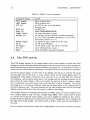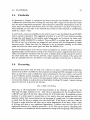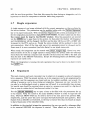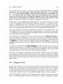
1
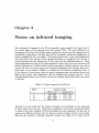
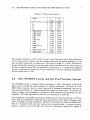
3 1. 08. 94
IRAC2
IRAC2
Operating Manual No. 20
ANDREA MONETI
April 1994
Contents
1 Introduction
2
2 Notes on infrared imaging
3
2.1
Standard stars
.
2.2
Science frames: object-sky pairs.
2.3
Selecting DIT, NDIT, and the number of object-sky pairs
3 Description of the instrument
4
4
4
..
5
6
3.1
The camera: optics and cryogenics
6
3.2
The NICMOS-3 array and the Pre-Processor System
7
3.3
The acquisition and control system
9
3.4
The Fabry-Perot unit
9
The f/35 photometer adapter
10
4.1
Optical arrangement
10
4.2
Source Acquisition
11
4.3
Autoguiding .
11
4.4
Commands
12
4..5 Command description
4.5.1
4.5.2
4.5.3
IF35
SET UP
I.
IMOVE GUIDEPROBE I.
IMAINTENANCE I ...
13
13
13
14
5
6
Observing
15
.5.1
Starting the acquisition system
15
5.2
The BASIC Acquisition Program
16
5.3
The PPS system
18
5.4
Biases and darks
20
5.5
Flatfields
21
5.6
Focussing
21
5.7
Single exposures
22
5.8
Sequences
..
22
5.9
Using the FP
23
5.10 At the end of the night.
24
System Performance
25
6.1
Broad band imaging photometry
........................
ii
25
List of Figures
4.1
Adapter softkeys . . . . . . . . . . . . . . . . . . . . . . . . . . . . . . . .. 12
5.1
PPS monitor display
.
19
5.2
Typical bias frame of :32 x 0.88 sec in ND mode..
20
iii
List of Tables
2.1
Typical intensity of the IR sky
3
3.1
IRAC-2 Objectives ..
6
3.2
Filters characteristics.
7
3.3
NICMOS-3 array characteristics.
8
4.1
F /35 User Commands . . . . . . . . . . . . . . . . . . . . . . . . . . . . .. 13
5.1
IRAC-2 User Commands. . . . . . . . . . . . . . . . . . . . . . . . . . . .. 18
6.1
Typical photometric ZP and net efficiency
25
6.2
Limiting sensitivities
26
.
1
Chapter 1
Introduction
IRAC-2 is a new infrared imaging camera equipped with a 2.16 X 256 pixel NICMOS-3
that is sensitive over 1-2.5 J.Lm spectral region. IRAC-2 has three functions that are
remotely controlled by the user: i) an objective wheel to select different pixel scales, ii)
a filter wheel containing the standard broadband and many Ilarrowballd filters, and iii)
an external (warm) scanning Fabry-Perot (FP) coated for the 2-2.5 J.Lm range and with
a resolving power of'" 1000. These functions make IRAC-2 a very versatile instrument
that can be used for many different scientific projects.
For the time being, IRAC-2 is controlled by a non-standard, BASIC acquisition system.
A new, more versatile and more efficient user interface will be installed by mid 1994. A
new version of this Manual describing the new system will be prepared then.
This document begins with a short introduction to the techniques of infrared imaging
(Chapter 2), then presents a detailed description of the camera system (Chapter 3) and of
the photometer adapters (Chapter 4), and finally describes how to actually use the camera
(Chapter 4).
Note that while there is reasonable experience with broadhand imaging, there is not so
much with narrowhand imaging, and rather little with imaging through the FP. Users of
these modes should come prepared to do some experimenting themselves to determine the
best way to observe, and any feedback to the author will be greately appreciated. Please
send any comments or corrections to the author ([email protected]).
2
Chapter 2
Notes on infrared imaging
The techniques of imaging in the IR are somewhat more complex than those used in
the optical region of the spectrum and with normal CCDs. The main difference is a
consequence of the fact that the IR emssion produced by the sky and the telescope can be
considerable, depending on the filter used and its bandwidth, making the background, or
loosely speaking the sky, very bright. The present system has to cope with backgrounds
that vary from a few adu/sec in the narrow-band filters or through the FP, and up to
several thousand adu Isec through the J( filter and with the wide-field objective. These
large backgrounds are such that a single integration of morc than just a few seconds would
saturate the detector. It follows that in order to accumulate sufficient photons, any control
system will have to acquire many such individual integrations and average them into a
final frame. In the context of IRAC-2, we define DIT, the Detector Integration Time, to
be the amount of time during which the signal is integrated onto the detector diodes, a.nd
NDlT as the number basic integrations that are obtained and averaged together. These
averaged frames make up the raw data, and are the smallest block of data tha.t is presented
to the user.
Table 2.1: Typical intensity of the IR sky
Filter
J
H
J(
Intensity range
[magiarcsec 2]
ADU larcsec2
150-400
15.0-16.0
12.8-13.6
1300-2800
11.3-12.1
3000-6000
Secondly, it is not unusual for the objects of interest to be hundreds or even thousands
of times fainter than the sky. Under these conditions it has become standard practice
to observe the source (together with the inevitable sky) and, separately, the sky, and to
perform the difference between the two frames to obtain a frame with the source alone.
Since the sky emission is typically somewhat variable (see Table 2.1 for typical sky in3
CHAPTER 2. NOTES ON INFRARED IMAGING
4
tensities), the only way to obtain good sky cancellation is by alternating rapidly between
source and sky and averaging together many such differences. This technique is called
bea.m switclIing. The switching frequency can depend on the nature of the source, the
integration time used, and on meteorlogical conditions. Ideally onc would like to switch
from object to sky more quickly than the time scale of the sky variations. While this could
be done with the traditional single-channel photometers, the overhea.d in observing with
cameras and the necessity of integrating sufficient photons to achieve background limited
observing conditions are such that the highest usable switching frequencies are of order
l/min and switching every 2-5 minutes is more typical. The beam switching technique
has the additional advantage that it automatically removes offsets due to fixed electronic
patterns (bias) and dark current.
As in the case of visible imaging, one must also correct for the intrinsic variations in
the pixel-to-pixel response. This is done by the use of flatfields, and the recommended
techniq ne is to obtain the flatfields on an illuminated dome panel and in differential mode,
i.e. images of both the illuminated and unilluminated dome panel are obtained with the
same OI!, and the flat field images are constructed from the difference of the two. In
this way the flat fields are obtained effectively in the same manner as the science frames.
This technique is especially important with the J( filter, where it will remove the thermal
component of the signal, whose amplitude does not depend on the intensity of the flatfield
lamp. To aid in this, a switch and a variac are available in the control room to switch the
.
lamp on/off and to control its intensity.
Some specific guidelines for the observations of different types of objects are given below.
2.1
Standard stars
Two or more images of the standard stars are obtained with a telescope shift in between.
In this way one image can be used as the reference for the other. If several images are
obtained, these can be used to check the uniformity of the flatfields. Most standard stars
are rather bright and it is often necessary to defocus somewhat. At present no sets of
standard star fields are available.
.
2.2
Science frames: object-sky pairs
The standard technique for the observation of scientific targets is to obtain one or more
object-sky pairs, depending on the brightness of the source and on the desired signalto-noise ratio (S/N). Unfortunately the sky frames always contain other stars, and by
Murphy's law one of these stars will fall on top of the object in the difference frame.
lt follows that some technique is necessary to artificially "remove" the stars from the
sky frames. The simplest method is to obtain several sky images, usually in the context
of several object-sky pairs, and then to stack filter them to produce a single sky image
without stars. This technique assumes that the sky fields are sufficiently uncrowded that
2..1. SELECTING OIT, NOIT, AND THE NUMBER. OF OBJECT-SKY PAIRS
5
on any given position of the array most of the images will have sky, and only a minority
will have a star. Clearly, a minimum of three sky images are necessary for this technique.
Another result of Murphy's law is that the source will inevitably fall on a bad pixel.
In many cases these bad pixels can be "fixed" by replacing them with the mean of the
surrounding, presumably good, pixels. This technique does not work, however, if the bad
pixels are clustered or if they fall in a region of rapidly varying intensity, such as the center
of a star. In this case it is best to obtain several object frames, again in the context of
the several object-sky pairs, with the object dithered (moved by small, random offsets) on
the array. Then, software techniques can be used to recombine the individual images in a
way that the bad pixels are rejected,
Generally, the separation between the object and the sky fields will have to be somewhat
larger than the size of the object. If the source is much smaller than the field of view, then
the sky can be chosen less than one array field away, as is normally done for the standard
stars. In this way the time spent on sky is also spent on the object, though the latter
appears in a different part of the array. If the object is larger than the field of view, it will
be necessary to scan the array over the object and then to combine the various images
into a single, large mosaic of the whole object.
2.3
Selecting DIT, NDIT, and the number of object-sky pairs
The appropriate value of OIT depends on the relative intensity of the source and the
background. First, and foremost, the OIT must be kept short enough that moderately
bright objects of scientific interest do not saturate.
On the other hand, in order to maximize the SIN, one would like to work in background
limited instrument performance (BLIP) conditions, Le. the sky intensity in a single frame
should be sufficiently high that the sky noise will dominate over the detector read-out
noise. In the J( band, where the sky is bright, this can be rea.ched with OITs of 1-10 sec,
depending on the pixel scale, but at Hand J, or through the narrowband filters, where
the background is lower, longer OITs would be necessary. Tt follows that the best value
of OIT is the longest possible that will not saturate the objects of interest.
Once OIT is chosen, NOIT can be determined from the desired beam switching frequency.
During good weather conditions one can stay on the object as long as 5 min before switching to the sky, and in this case NOIT = 5 min I OIT is appropriate. If conditions are not
so good, e.g. the sky intensity is fluctuating rapidly, or if one simply does not wish to
integrate that long, then a lower value of NOITcan be used.
Finally, the total number of object-sky pairs to be obtained will depend on how deep one
wishes to reach (and on how much time onc has available).
Chapter 3
Description of the instrument
3.1
The camera: optics and cryogenics
The IRAC-2 camera is housed in a modified Oxford Instruments liquid helium cryostat.
Light enters the cryostat through an aspheric, 70 mm, field lens mounted on the side of
the cryostat which thus doubles as the input window. This lens forms an image of the
telescope pupil on a 4.5 mm pupil stop that limits the amount of stray light that enters
the system. Following the pupil stop is the lellS wheel that carries five objectives which are
used to re-image the field onto the array at different pixel scales. Table 3.1 summarizes
the pixel scales available and the corresponding field sizes. For the largest pixel sizes the
field of view is limited by the entrance window to a diameter of 180".
Table 3.1: IRAC-2 Objectives
Objective
Name
A
B
C
D
E
Scale
[Arcsec/pix]
0.153
0.27
0.49
0.70
1.10
Field size
[arcsec]
39 X 39
69 x 69
1~j3 X 133
<I>
180
<I>
180
=
=
In front of the pupil stop is a 24-position filter wheel that carries the standard JHK
filters, a special/(I filter, and many narrow-band filters. A list of these filters and their
characteristics is presented in Table 3.2. The /(' filter is intended for deep imagillg and
it is designed to avoid the thermal emission that occurs to the red end of the standard
/( filter. At 13 C the sky + telescope background through the /(' filter is 35% lower
than through the standard /( filter, yieling a 20% reduction in the sky noise. The noise
reduction is greater at higher temperatures, but the night t<lmperatnre is rarely higher
than about 15 C at La Silla.
G
3.2. THE NICMOS-3 ARRAY AND THE PRE-PROCESSOR SYSTEM
7
Table 3.2: Filters characteristics
Name
J
H
K'
K
NB1 (Fell)
NB2 (Fell)
NB3 (HeI)
NB4
NB5 Oh)
NB6
NB7
NB8 (Br-I')
NB9
NB10 (CO-cont.)
NBll (CO)
1.25
1.6.5
2.1.5
2.2
1.262
1.645
2.058
2.105
2.121
2.136
2.148
2.164
2.177
2.216
2.365
0.30
0.30
0.32
0.4
0.04
0.0,1
0.036
0.037
0.039
0.038
0.037
0.037
0.038
0.075
0.088
The cryostat contains an "outer" and an "inner" tank. The outer tank is filled with liquid
N2 (at 77 K), and it is used to cool the radiation shield and the optical assembly (Le. the
lens and filter wheels and the pupil stop). The latter is cooled to '" 105 K. The detector
mount is thermally connected to the inner tank which is also filled with N2 , but in this case
the N2 is cooled to below 70 K and solidified by pumping on it. A temperature regulator
is used to maintain the detector at a fixed temperature. The best operating temperature
for the current array is 70 K.
3.2
The NICMOS-3 array and the Pre-Processor System
The NICMOS-3 array is a hybrid device consisting of a 256 x 256 matrix of Hg:Cd:Te
diodes that is bonded via indium bumps to a readout multiplexer. The latter is of the
DRO (direct read-out) type, in which each pixel is addressed individually and can be
read non-destructively, Le. without clearing the charge out of the array. To increase the
speed of readout, the multiplexer is structured in four quadrants having separate output
amplifiers. The basic properties of the array are summarized in Table 3.3.
The multiplexer is controlled and read by a VME-based Prc-Processor System, or PPS for
short, that was developed by ESO and which contains four 16-bit ADC's allowing simultaneolls reading of the four quadrants. The PPS is controlled by a Motorola 68040-based
Eltec E-7 computer which also runs various data processing tasks. It receives detectorspecific command and control files from the host workstation, displays the images in
8
CHAPTER 3. DESCRIPTION OF TIlE INSTRUMENT
Table 3.3: NICMOS-3 array characteristics
Format
Pixel size
Operating temperature
Dark Current
Well depth
Read nose
Quantum efficiency
No. of bad pixels
Overall uniformity
2.56 x 2.56
40/lm
'" 70 K
'" 1 e- /sec
105 e -
'" 35 e40% at 1.21lm; 60% at 2.2/lm
'" 500 « 1%)
'" 15% RMS
real-time, performs the necessary averaging, optionally computes rms noise images, and
transmits the final results back to the host.
Several readout modes are available and can be easily selected from the control program.
Each readout mode consists of one of more detector READs, and it is important to know
that these READs are all non-destructive, i.e. reading the value of a pixel does not imply
resetting it, as is the case in optical CCDs. With this array, as with many IR arrays,
the resetting action is independent of the reading, and this feature gives the builder the
possibility of devising many different and powerful readout schemes.
Two readout modes are available for general observations: double-correlated sampling
(also known as RESET-READ-READ) and multiple non-destructive (ND) readout. In the
former mode, the array is read twice (non-destructively) at the beginning and at the end
of the integration. The signal is computed as the difference between the end and the
start READs. This mode produces bias frames that have a large, but stable, negative value
(about -1000 ADUs); this offset may come from some interplay between the reset that
preceeds the integration and the first READ. The minimum DIT in this mode is 0.55 msec.
In ND mode a reset of the array is followed by a first READ, which is discarded, and then
by a series of READ / delay until the detector integration time, DIT, is over. Each READ takes
227 msec and is followed by a delay which is at least 100 msec and whose length depends
on DIT: for short DITs the minimum delay is used; for longer OITs the delay is increased
dynamically in order to maintain the number of reads to a maximum of 20. Finally,
750 msec are used to compute a linear regression fit for each pixel, and the resulting slope
is multiplied by DIT to give the total signaL The minimum DIT in this mode is 0.881 msec.
The important advantage of the ND mode is that it results in ,dower effective readout noise
but at a cost of some time overhead. It should be used under low background observing
conditions, when the DITs are long ( ~ 20 sec) and the overheads become unimportant.
Under high background conditions, the double-correlated mode should be used since it is
more efficient, and since the noise is entirely coming from the background any reduction
in readout noise could not be noticed.
.1.3. THE ACQUISITION AND CONTROL S1'STEM
For more details on the read modes and on the other tasks performed by the PPS, see the
"Infrared Pre-processing System PPS" Version 2.0 (April 1992) by Peter Biereichel.
3.3
The acquisition and control system
At the present time the camera and the detector are controlled via a BASIC program
running on an HP360 host workstation. The HP360 is interfaced i) to PPS, ii) a CAMAC module to control the moving functions (filter, lens, and FP wheels), iii) to the FP
controller, iv) to the instrument HP1000 computer to control some photometer adapter
functions and, indirectly, some telescope functions, and finally v) to an HP730 workstatioIl
which receives the data and is used for on-line data analysis (with MIDAS).
Communication between the HP360, the HP730 and the PPS runs through an local Ethernet network, and the HP730 is also connected to the- general mouutain Ethernet network
though a second Ethernet port. Communication to the UP1000 computers is achieved
through an RS-232 serial link, and is used to retrieve telescope position, focus, UT and
ST, and other parameters that are then stored in the FITS image headers. There is also
a mode of operation which allows the HP360 to control the telescope and the autoguider.
This system is to be replaced in the near future by a more versatile, Unix-based, one. The
new system will be described in a latcr release of the Manual.
3.4
The Fabry-Perot unit
A warm Fabry-Perot (FP, Queensgate Instruments model ET 70 WF) for use in the ]tband is available to use with IRAC-2. The FP is located in a remotely controlled "FP"
wheel in front of the camera. That wheel has three positions of which one is open for
direct observations. The last position will be used for an H-band FP in the future; at
present it holds a mask that can be used with lens B to reduce the incident background.
The throughput of the FP varies between 70 and 80% over the 2.0 to 2.51tm range; the
measured finesse is > 50 for 2.04 Itm < A < 2.46 /lm, and> 40 for 2.00 /lm < A < 2.60,,,m.
The finesse degrades rapidly outside the latter range, and it is ouly 33 at 2.65Itm.
The FP is intended for line imaging rather than for line profile studies; it has a resolving
power of AII::i.A ~ 1000, which gives a velocity resolution of 300 km S-l. The narrow-band
filters are normally used for order selection.
The wavelength calibration of the FP is checked by the moutain staff before its use using
a spectral line lamp. Since the FP is out in the air, air wavelengths are used rather
than vacuum wavelengths. The index of refraction of air at 2.01Lm is 1.000273 (from
Lang, Astrophysical Formulae). Users are still advised to check the calibration on an
astronomical source.
.
Chapter 4
The f/35 photometer adapter
The f/35 photometer adapter at 2.2 m telescope was originally designed to interface the
InSb photometer and the bolometer to the telescope and to provide for object acquisition,
offset guiding, and to control the chopping secondary. IRAC-2 is normally mounted on
the bolometer side of the adapter and with the adapter rotated to P A 90~ which brings
IRAC-2 to the south side of the telescope, which is the most convenient position for
accessing the instrument.
=
Normally a night assistant is present and is responsible for pointing the telescope and
guiding, hence he will worry about the various adapter functions. The short description of
the adapter system given here is not intended to be complete (see the Infrared Photometers
User's Manual, Bouchet 1990, for that), but it is meant to describe the functions needed
for IRAC-2 users, Le. the control of the dichroics and of the guide probe.
4.1
Optical arrangenlent
The infrared beam is directed to either of the two detectors by a ,15 0 pick-off mirror.
About 1% ofthe visible light is transmitted by the that mirror, so that stars brighter than
R ~ 10 mag can be seen through it. There are in fact two such mirrors, each of which
directs the light to one side of the adapter. These are supported on arms so that the
centre of the field is either unobstructed (for acquisition of faint objects) or occupied by
the appropriate one. For historical reasons these mirrors will be called the dichroics in the
following text.
The acquisition/guiding system employs a fixed TV camera which views the field via one
of two objectives, a small flat mirror, and a field mirror in the focal plane of the telescope.
The two objectives give instantaneous fields of view of 6~3 X 9~5 (large field) and 1~6 x 2~4
(small field). By tilting the small flat guide-probe mirror these fields can be moved over a
16' diameter field. An optical cross-hair is projected onto the TV camera. This cross has
a "gap" in the center of 5" x 5".
10
4.2. SOURCE ACQUISITION
11
The field is normally imaged on a Bosch ISIT sensitive up to 8500 A; various filters can be
positioned in front of the TV cameras, though nearly all the time t.he open position (no
filter, this is the default) turns out to be most convenient.
4.2
Source Acquisition
The same TV camera is used for center-field viewing and for offset guiding. A center
position is normally determined and stored before the start of observations such that the
center of the light cross is coincident with the center of the infrared field. As the center
field can be viewed either directly or through the pick-off mirror, there are in fact two
center positions that should be determined since the mirror introduces a shift of'" 10" in
the optical.
The center positions are determined by first centering a moderately bright star ou the
array (hence the dichroic must be inserted), then moving the guide probe with ~ and
~ until the star is in the center of the light cross, and finally storing the dichroic in
center position with STORE eTR pas. Fast and slow guide probe speeds are available,
and one can toggle them with FAST/SLOW. Next, the dichroic should be moved out of
the beam, which will produce an apparent displacement of the stellar image of '" 10" due
to the refraction within the dichroic, the light cross should be recentered onto the star,
and the new center position can be stored for the out position of the dichroic. Only one
STORE CTR pas command is available, and the system knows whether the dichroic is
in or out and thus will store the guide probe position accordingly. Similarly, when the
GO TO CENTER command is issued, the system will check whether the dichroic is in or
out and then will move the guide probe to the corresponding center position.
I
I
I
I
The philosophy behind this system is that one could center faiut objects onto the Hght
cross with the dichroic out, then insert the dichroic and have the source onto the rather
small aperture of the photometers. With the camera one can often acquire the source
directly in the infrared using the ou-line display and it is usually 1101. necessary to move
the dichroic out of the beam. Nevertheless it is convenient to define the center positions
as described above in order to have a reference of where the center of the field is located
on the sky. Note that the centers of the fields of the IRAC-2 objectives are not exactly
coincident, though they do He within'" 10" of each other.
4.3
Autoguiding
Once the object is acquired and placed in the desired position of the array, one can proceed
to find a guide star. This is best done by first moving to the large field, locating a suitable
star, then moving the guide probe so as to bring the star near the center of the field (Le.
the light cross). Then, upon moving back to small field, the star will be in the field, and
the guide box (from the TCS) can be moved on top of the star and the autoguider started.
CHAPTER 4. THE F/35 PHOTOMETER ADAPTER
12
MOVE GUIDEPROBE
X-hair brighter
CHOP2
Help
F/35 SET-UP
X-hair darker
MAINTENANCE
TERMINATE
Store ctr pos
Store guide star
X-hair brighter
-ETC-
Goto ctr pas
Goto guide star
X-hair darker
PREVIOUS MENU
Move Y+
Move X+
Delta X,Y
-ETC-
Move Y-
Move X-
Scan Guidestar
Fast<->Slow
Bolometer
Dichroic in
Small field
Move .filter
InSb detector
Dichoric out
Large field
PREVIOUS MENU
Goto park posn.
Update param' s
Guideprobe speed
Displ gd-stars
Init.
Calibr.
motors
table
PREVIOUS MENU
Figure 4.1: Adapter softkeys
4.4
Commands
The program controlling the guide probe at the 2.2 m is called F/35, and this name should
appear in the center of a line just below the graphical display of the softkeys. If it does
not, it should appear as one of the softkeys; in this case, press that softkey to gain control
of the program.
A diagram of the softkey tree is shown in Fig. 4.1. The top row of that figure corresponds
to the eight softkeys of the main menu. From here, IMOVE GUIDEPROBE I will enable the
second row of softkeys, /35 SET-UP will enable the fourth row, and MAINTENANCE will
enable the last row. From the second row, I-ETC-I will move to the third row, and the
I-ETC-I in that row will move back to the second row. Most of the time only the second
and third row are used, and typed commands are used to move the dichroic in and out,
and to switch between small and large field. The commonly used typed commands arc
listd in Table 4.1. A complete list of available typed commands can be obtained on the
screen by typing "??".
IF
I
I
I
13
4..5. COMMAND DESCRIPTION
Table 4.1: F/35 User Commands
Command syntax
o I or 0,1
o 0 or 0,0
LF
SF
BOLD
INSB
FI,n
4.5
Command description
4.5.1
IF35 SET
Action
dichroic in
dichroic out
go to large field
go to small field
set bolometer detector
set lnSb detector
set TV filter n
upl
By selecting IInSb Ior IBolometer I, one selects whether the lnSb or the Bolometer side of
the adapter is used and hence which of the two dichroics is moved into the beam to direct
the light to the instrument. As mentioned earlier, lRAC-2 is mounted on the bolometer
side. Other softkeys are available to change between small and large field, to move the
dichroic in and out, and to place a filter in front of the acquisition camera. Upon starting
the program the bolometer side is selected automatically, and the other functions are
activated more conveniently via typed commands, so this menu is practically nevery used.
4.5.2
IMOVE GUIDEPROBE!
This menu contains the keys to handle the guide probe and the light cross. The current
position of the guide probe can be stored as the center position with IStore ctr pos I,
and it can be moved back to that position with Gete ctr pos Two buffers are available
for the center positions with the dichroic in and out of the earn, respectively. When
executing either of those commands the system first checks the position of the dichroic
and then stores of goes to the appropriate one.
I
t
The guide probe position of a guide star eau be stored with STORE GUIDESTAR followed by an integer. This position can be recovered later with GO TO GUIDESTAR followed by the same number. The list of stored guide stars can be displayed by pressing
10ISPLAY GUIDESTAR in the MAINTENANCE menu.
I
I
I
The guide probe can be moved manually with the ± X and ± Y keys, and a fast and
a slow speed are available and can be toggled with the fast<->slow key. To move the
guide robe push one of the motion keys and hold it until the star arrives at the desired
location, then release it. If moving at high speed the guid probe will overshoot and then
come back to where it was when the key was released. Wait for the terminal's BEEP
14
CHAPTER. 4. THE F/35 PHOTOMETER. ADAPTER
before proceeding with other motions. The BEEP indicates that t.he system is ready
for the next command. X, Y encoder readings arc updated on the screen when the key
is released. Small movements can be made by hitting the key twice rapidly. In moving
the probe, note that the program does not know the position angle of the adapter on the
telescope flange. With IRAC-2 it turns out that [IT] and \}:JJ move the guide probe
north-south and east-west, respectively. The fast and slow speeds can be programmed
from the MAINTENANCE menu (see below)
I
Searching for guide stars can be performed as described earlier or using the SCAN GUIDESTAR
key. Holding that key pressed will cause the guide probe to execute a. rectangular raster
over the field. Releasing the key stops the scan. The star can then be centered using the
[ITJ and \}:JJ keys.
An offset in RA and/or DEC can be applied to the guide probe with the Delta X. Y
softkey. That key will open a screen asking for the offsets; type the desired ofI'stes both
must be in arcsec!) and apply them with the ENTER key. Once again, since the program
does not know the position angle of the a.dapter, asking for an offset in RA will actually
move the guide probe in DEC and vice versa. In practice this key is rarely used.
I
I
I
Finally, the illumination of 1, he optical cross can be adjusted by pressing X-hair brighter
I
or IX-hair darker I.
4.5.3
IMAINTENANCE I
I
This menu contains only two keys that are useful to the IRAC-2 users: Guideprobe speed
to set the fast and slow speeds of the guide probe values of 4.cO" /sec and 4" /sec, respectively, are typical for IRAC-2), and Init . motors to initialize the motors, should some
problem occur.
I
I
Chapter 5
Observing
5.1
Starting the acquisition system
The system will generally be set up by the IR Operations Group. Should it be necessary,
however, the following steps can be followed to login and start the system:
• On the X-terminal:
1. select host ir22 by double clicking on it;
2. when the login window appears, login with username irac2 and with password
irac..2. Then wait for the HP Visual User Environment (VUE) to start the IRAC-2
and SYSTEM workspaces;
3. select the IRAC-2 workspace by clicking its bar on the control panel
4. click on the RMB symbol on the control panel to start the BASIC program, and wait
for the BASIC window to appear; make sure that only one RMB icon is displayed
on the lower-right corner of the screen;
5. type LOAD IIRAC2B" to load the control program, and then RUN to start it running
(note the capital letters!). At this point the program will prompt for the user's name,
for a short description of the project, and for a 2-4 letter code to use as the root for
the name of the images, and for which the user's initials (in small letters) are often
chosen.
At this point the motors and the PPS will be initialized, a status window will appear, and
a softkey menu will appear at the bottom of the BASIC window.
• On the HP730 console:
1. login with username irac2 and with password irac..2, as before, and watch for the
creation of three workspaces labeled "Midas-IRAC-2", "Midas- User", and "Scratch
workspace"j
15
CHAPTER 5. OBSERVING
16
2. in the "Midas-IRAC-2" works pace: i) move to the rock sub directory with the Unix
command y'cd rock, ii) start Midas with Y.inmidas 00, which will automatically
create a display and a graphics window, and once in Midas give the command pps
to transfer control to the HP 360 host.
3. in the "Midas-User" workspace: repeat step i) above, then ii) start Midas with
Y.inmidas 01, which will automatically create a display and a graphics window, and
also initialize some special commands.
Two other programs must be started on the HP1000 "instrument" computer: the f/3.5
program that controls the f/35 chopping secondary and the photometer adapter, and the
IRAC2 program which manages the communication between the HP 1000 and the HP360
workstation. To start these programs,
1. login with username IRAC2F35 on the LU72 terminal and follow instructions. When
finished, check that the filter is set to whit, and if this is not the case type the
command FIL 1.
2. once the IRAC2F35 program is running login with username IRAC2 on LU12, and
that program will start.
When starting both of these programs, the user will be prompted for a confirmation soon
after logon. This can be done by either pressing the F1 softkey or by physically typing
RETURN. At this point everything should be running properly, and the user is ready to
start.
In case of a crash of the acquisition program it is not necessary to restart the whole
system. In nearly all cases it is possible to reset the BASIC with the green shift-reset key
(upper left of the keyboard) and then either typing RUN of pressing the RUN softkey, if it
appears. At this point the user will be prompted once again for the start-up information,
and typing just (er) will reuse the previous ones.
I I
5.2
The BASIC Acquisition Program
Upon startup the BASIC acquisition program presents the user with a control window
from which the camera is operated, a status window, and possibly a window with a plot
of the FP calibration curve.
At the bottom of the control window is a menu consisting of eight softkeys which are
described below. These keys can be activated either by clicking on them with the mouse
or by physically pressing the corresponding key located along the top of the keyboard.
I
I
I
1. The auxiliary menu has Init .
I
I
I
I
Motors and Init PPS softkeys for re-initiali-
zing the motors and the PPS, an EXIT MIDAS Ikey to properly terminate the IRAC-2
17
5.2. THE BASIC ACQUISITION PROGRAM
I
I
Midas session on the HP 730, a Display Image key to display an image on the
monitor (actually this key is not implemented; a any rate during regular observations
since Midas is used instead) a Filter Autom. key to toggle on and off the automatic
selection of best order-sorting filter when using the FP, a IFilter Curve key to
toggle on and off the drawing of the selected FP orders and the order-sorting filter
profile, again when using the FP, a Snapshot mode to enable a special mode which,
I
I
I
I
I
however, is not yet implemented, and finally an @BSERV. MENU Ikey to return to the
main menu.
I
I
I
.1
I
.1
2. The PPS menu has Store Fixed Patt and Clear Fixed Patt keys to store
the current image in the PPS buffer iuto a Fixed Pattern buffer so that such a fixed
pattern can be subtracted from all the subsequent images until it. is cleared. This is
most useful for performing "on-line" sky subtraction. Then there is an Autocuts
key which sets the PPS display cuts to values based on the pixel values in the
current image, a DISPLAY PARAMS key to interactively send cut values and other
parameters to the PPS (very seldomly used), and finally an I OBSERV. MENU key to
return to the main menu. Note that storing/clearing the fixed pattern and applying
the automatic cuts-is much more conveniently done from the mouse buttons on the
PPS monitor (see next Section), and consequently this menu is seldomly used.
I
I
I
.1
I
I
I
3. The FOCUS menu has provisions to do a focus sequence, but experience has shown
that this is not the most efficient way to focus; focussing is discussed in more detail
below.
4. A Peakup Signal softkey to (re)start the continuous display of every single frame
as It IS acquue
y the PPS. This key is rarely used since the continuous display
mode is enabled automatically upon startup and upon termination of an exposure.
It is not started automatically, however, following an ABORT of an exposure, and
on some occasion it stops when activating the fpat I key of the PPS.
I
I
I
I
I
I
I
5. The Define Exposure and Define Sequence keys to set the parameters for a
I
single exposure and for a sequence of up to 10 exposures, and the Start Exposure
I
I
I
and Start Sequence keys to start them.
I
I
During an integration the ABORT key becomes available for interrupting the measurement.
Once the measurement is aborted it cannot be continued.
I
I
The Def ine Exposure and Def ine Sequence softkeys open a new window containing
a form or table to be filled wit t le re evant parameters. Note that to type into the fields
the cursor must be in the BASIC window rather than in the form window.
In addition to the softkeys, many operations can be done via typed commands. These are
often quicker and more convenient than entering parameters in windows. Typed commands
can be used only from the main menu, and none can be given while an integra.tion is
running. A list of typed commands is given in Table5.1; this same list can he obtained on
the terminal by typing "?".
18
CHAPTER.5. OBSERVING
Table 5.1: IRAC-2 User Commands
Command syntax
FILT [name]
LENS [name]
OIT [n]
NOIT [n]
NINT [n]
IDENT [text]
NCOORS [n]
ETYPE [type]
FP [A
FP [posn]
FOC [i]
EXIT
5.3
Action
Move to given filter
Move to given lens
set OIT to n sec or to the closest
possible value
set NOIT to 71
NOT IMPLEMENTED
set image identifier to [text]
set the read mode t.o Double correlated sampling
(n = 2), Triple correlated sampling (11. = 3), or nondestructive readout (n = 4)
set exposure type, Le DK, CAL, FF, Sel
set FP to wavelength A
set FP wheel to pos. IN, OUT, or MASI(
move telescope focus to pos. i
exits the BASIC acquisition program
The PPS system
The PPS display consists of two image displays and a zoom window, several data fields
displaying various detector-related parameters and the status of the current integration,
and several buttons to control the user fuctions; see Figure .5.1,. A three-button mouse is
used to activate the buttons on the display. The three buttons on the mouse are equivalent.
Of the two square regions in the center of the display, the left one is used for the image
and the right one for the noise. A zoom window above the left image display shows an
enlargement of the region around the cursor and, next to it, is a data. field that indicated
the minimum and maximum pixel values, the average and the standard deviation of the
pixel within the zoom window. This is very useful, for instance, to check whether a bright
star is saturated, to see the mean level of the sky, and to aid in focussing. Just below
the image is a 9 x 9 array of numbers, these are the pixel values at the cursor positions
and the 8 adjacent ones. The zoom window and the pixel display exist only for the image
display and are active only when the cursor is inside on the image.
Two display modes are available, denoted OIT and NOIT, which are used to display every
basic readout (OIT) or only the final, average image (NOIT). The current mode is shown
in a button above the left image display, and can be toggled by clicking on that button.
In NOIT mode an RMS frame is computed from the basic integrations and is displayed in
the right-hand image display. The default mode is OIT, in which case the noise display is
not used.
Near the bottom and top left corners of the image display are two pairs of buttons, marked
HCUTl
~
,- - - - - -: Max: 6470.3
:
I Min: 325.33
:
: Ave: 4329.4
:
: StDev: 955.3
:----------------------i
I
I
I
I
I
I
I
I
I
I
I
I
I
I
I
I
: NOISE
I
:
I
,
I
I
I
I
I
I
I
I
I
I
I
I
~I
~i
I
IMAGE
i
I
I
I
I
I
I
I
I
I
I
la
-----------------------1HCUT2
I
I
~I
LCUTl
UT 03:22:38
I
I
I
I
I
I
I
I
I
I
I
I
I
,-----------------------
XC=133 YC=199
LCUT2
--------------------------------------------------------I
I
I
I
:
I
Status display
:
I
1
I
-----------------------------------------------
_
T=69.9 t=102.4
Figure 5.1: PPS monitor display
[±] and [:=J, which are used to increase and decrease the high and low cut levels of the
display. The two buttons labeled Iacut I and Ifpat Iare used to set the display cuts to
values automatically determined from the statistics ofthe image, and to set/clear the fixed
pattern buffer. The latter is very useful to do on-line sky subtraction when, for instance,
acquiring a faint object. The fixed pattern buffer can be "set" to hold an image, and this
image will be subtracted from all subsequent images being displayed. When "setting" the
fixed pattern, the image currently on the display will be stored in the buffer. At this point
the button changes color from yellow to green, and a message appears indicating that a
fixed pattern is stored. When "clearing" the buffer, the contents of the buffer are set to
zero, the button changes back to yellow, and a message appears indicating that a fixed
pattern is cleared. Setting and clearing the fixed pattern only affects the display; the data
that is transfered to the host at the end of the integration is always the raw data.
A v:ertical color strip appears at the extreme left ofthe display; clicking on this will activate
different color look-up tables and a grey-scale one.
The data fields below the image and noise displays indicate the integration parameters,
the status of tlle current integration (total and remaining integration time), detector and
optics temperature, and other, self-explanatory data.
CHAPTER 5.
20
OBSF:RVJNG
Figure 5.2: Typical bias frame of 32 x 0.88 sec in ND mode.
5.4
Biases and darks
Biases and darks may be obtained with the DK filter which blocks off incoming light.
Since the dark current is quite low and observations aTe normally done in differentia.l
mode, dark frames are not always llsefuL On the other hand, bias frames can be used to
measure the read noise and thus check that the array, and indeed the whole system, is
working properly. The read noise can be measured from the rrns pixel-to pixeJ variation
in the difference of two bias frames. The most convenient way to do this is to use the
VIEW /IMAGE command in MIDAS. Assuming thc system is ergodic, thL value wj]] be
t.he same as the rms of many individa.l merLsurements on a single pixel. If the bia.s frames
a.re th average of NDIT individual images, the read noise is given by
RON
= JNDIT
~
RMS
wher RMS is the rms pixel-to pixel variation in the differcnce framc. This value should bc
about 7 DU and if it is significantly higher it indicates that something is not working
properly.
A sample bias frame obtained in ND mode is shown in Figure .5.2. The signal level near
the center of the frame is .5-10 ADD, and the glow of the output amplifiers is clearly visible
in the corncrs.
21
5.5. FLATFIELDS
5.5
Flatfields
As discussed in Chapter 2, experience has shown that the best flatfields are obtained in
a differential mode from pairs of lamp ON and lamp OFF images of the dome fiat taken
with the same integration parameters. This technique is especially advantageous in the J(
band, where the thermal contribution from the warm telescope is canceled. Furthermore,
these fiatfields are more akin to the scientific data which are also obtained in a differential
mode (Le. object - sky).
A switch and a variac are available in the control room to turn the fiatfield lamp ONjOFF
and to control its intensity. The suggested procedure is to set OIT to its shortest possible
setting (this will depend on the readout mode being used), and to adjust the variac until
a signal of 8,000-10,000ADU is reached. Then set NOIT to a. rather high value, typically
60-100, so that lots of photons are integrated, and proceed with the integration in single
exposure mode. Make sure that the telescope is set up properly pointing to the dome
panel and with the mirror cover open, and that the dichroic is in.
The best fiatfields appear to be the ones taken through lens Le. Lenses LA and LU produce
significant light concentrations (a peak in the renter for LA and a ring for LU) that do not
reflect the sensitivity variations over the array. It follows that LC fiats should be used for
the other lenses also. For lens LD, however, which vignetts the corners of the array, LD
fiats are probably the best, but there is very little experience with that lens at this time.
5.6
Focussing
Experience has shown that the best way to focus is to point a crowded field (a globular
cluster such as M14 is excellent for this purpose) and using the FOC command to move the
focus up and down until a satisfactory value is determined. For best results, use lens LB
to have sufficient spacial sampling, set OIT to 5 sec or more in order to average seeing at
least to some extent, store a sky in the fixed pattern buffer, and examine several readouts
on the on-line display at a given focus setting before deciding if it is good. A good starting
value for the focus is given by the formula
foe = 2549
+ 51.25 TLS,
where TLS is the temperature of the long serurriers of th(' telescope as read from the
TCS (ask the night assistant for it). This value is appropriate for the hroadband filters
(J H K K') and lens LB; the best value for lens LC is 20 steps lower. In analyzing a focus
position it is often easier to concentrate on two nearby stars and noting how well they
separate, rather than concentrating on the sharpness of a single star. It is also important
to check that the focus is uniform over the whole field. If the focus is well set, a shift of
20 steps in either direction will show only a minor degradation of the focus, while a shift
of 40 steps will show a very significant degradation. It follows that the focus has to be
readjusted whenever TLS varies by more that"" 0.4 C. This can be done by calculating the
offset necessary to compensate for the temperature change and then giving a Foe command
CHAPTER 5. OBSERVING
22
with the new focus position. Note that this cannot be done during an integratioll, so it is
important to check for temperature variation before long exposures.
5.7
Single exposures
A single exposure is an image obtained with the current parameters as they are listed in
the 'status window. The parameters can be modified either with the Define Exposure]
I
key or via typed commands. With the Define Exposure key a form prompting the user
for the integration parameters is displaye m a new wm ow. To enter values into the form
the cursor must be kept in the BASIC window. Once the parameters are entered
use the ENTER key to pass them to the system. At that point the window will disappear
and the parameters will be changed: the filter and the lens
be set, DIT ..,.lId NDIT will
be passed to the PPS, and so on. Finally the status window will be updated to show the
new parameters. Most of the time only one or two parameters must be cha.llc;ed, and in
those cases it is more convenient (and also faster) to use typed commn,nds.
I
I
will
When ready, the integration can be started with Start single exp . There is an overhead of about 25 sec for a single exposure during w IC t le system reads the telescope
status fx:om the telescope computer and transfers the data from the PPS to the host and
from the host to the MIDAS workstation. Except for obtaining biases and fla.t.fields, single
exposures are rarely used.
While the integration is running the only operation that can be done is to abort it with
the ABORT key.
I
I
5.8
Sequences
The most common and most convenient way to observe is to program a series of exposures
into a sequence. With the present system, up to ten exposures can be pre-programmed in
a sequence, and the sequences are stored and can be recalled, modified, and reused. No
editing of sequences can be done during an integration. Sequences are very ven:;atile but
can also be a double-edged sword: a proper use will result in a considerable time savings,
but special care should be exercised since an error in a sequence can result in a big loss of
time or even in useless data if one does not notice it in time.
I
I
Use the DEFINE SEQUENCE key to open a form to be filled with the parameters for up
to ten frames. Keep the cursor in the main (BASIC) window in order to type into the
form. TAB and SHIFT-TAB can be used to move to the next and to the previous field,
respectively, and the arrow key move one space forward/ba.ckwards a.nd up/do\\·n. Only
frames with an identifier are executed, so the way to execute less than ten frames is simply
to leave blank some of the identifier fields.
In addition to the standard integration parameters, the user can specify a telescope offset
to be executed BEFORE the exposure is started. These offsets are in arcsec in both
23
5.9. USING THE FP
RA and DEC, and are relative to the current position. Note that due to a preload
problem in the 2.2 m telescope's delta axis, offsets south of '" -65° and north
of '" +15° are not always reliable. The symptom is that some of the offsets can
be '" 10" shorter than the desired value, and that offsetting north and then
south (or vice-versa) may not bring the telescope back to the same position.
Thus users are encouraged to use offsets in RA only when observing far to the
south. In particular, this can be a nuisance for Magellanic Cloud work.
Finally, there is an "autoguider flag" which must be set to Y or N, and which cau be used
to start the autoguider before starting the integration. Setting it to Y assumes that the
sequence is programmed in such a way that a sta.r will fall into the guide box for that
exposure. If that is not the case, for instance if the sequence is programmed to dither the
obj~ct, the autoguider flag should be left to N and the autoguider started manually.
The one parameter that cannot be changed from a sequence is the telescope focus. This
will change in the new user interface that is being developed. At present this means that
it is unfeasable to program observations with different lenses 01' with and without the FP,
since these require focus adjustments.
I
I
Once the sequence is programmed it can be stored in a file with the Enter on file key,
which will prompt for the file name. That name can be either a new one or one that is
already in use, in which case the previous sequence will be overwritten. Alternatively, with
the IENTER key it will be stored in the default sequence file, SEQ-PARAMS. It is common to
program some sequences to be used as templates, and then to edit these for each particular
situation.
I
A sequence is started with the START SEQUENCE key, which will prompt for the user for
the name of the sequence to be starte . As a default, the last sequence that was addressed
will be proposed. Type the name of the desired sequence followed by CR, or just a CR if
the default sequence is the correct one, and the sequence will begin.
Note that upon starting an integration no internal check is made to see if the telescope
can continue tracking for the necessary amount of time without running into its limits.
When observing far to the west or dose to the pole, the telescope can run into the Zenith
Distance (70°) and Hour-Angle (6 hr) limits respectively. If in doubt, users should ask the
night assistant.
5.9
Using the FP
The FP can be placed in the beam with the typed command FP IN and removed with
FP OUT. Due to the change in the optical path when the FP is inserted, it is necessary
to lower the telescope focus by 50 steps when the FP is inserted. The FP can also be
inserted/removed from the exposure and sequence setup forms. The latter, however, is
not practical at present since it is not possible to cha.nge the focus within a sequence.
The FP wavelength is usually set in the sequence form, though it can also be set manually via the FP nnnn typed command, where nnnn is the d<,sired wavelength in microns.
CHAPTER 5. OBSERVING
24
Imaging with the FP produces a background with large spatial variations, and these variations arc somewhat wavelength dependent. As a consequence a. good image can only be
obtained using the same (object - sky) technique discussed earlier for broadballd work.
It follows that to obtain an image in a line, an (object - sky) pair at the line wavelength
and another one at a nearby continuum wavelength must be obtained. Since the system
can have different throughputs at the two wavelengths, the two images must be properly
normalized before subtraction. Scanning the FP is possible by programming a sequence
with different wavelengths.
When using the FP the user has the options of (i) having the system determine the correct
order selection filter and set it automatically, and (ii) to have a plot drawn with the filter
transmission curve and the position of the FP orders. These options can be toggled on
or off with the Filter Autom.1 and Filter Curve softkeys in the Auxiliary menu.
Normally both these options are set.
I
5.10
I
I
I
I
At the end of the night
At the end of the night
1. Put in the dark filter by typing FIL OK in order to protect the array from stray light.
2. Exit the program with the EXIT command.
3. Fill out the night report.
At present the IR Operations Group will worry about transfering the data from disk to
DAT tape.
Chapter 6
System Performance
6.1
Broad band imaging photometry
Photometric zero-points (ZPs) for broadband photometry, defined as 2.5 10g(CFZAf) , and
where CFZM are the counts for a zero-magnitude star, are listed in Table 6.1. These
values were derived for lens LB, and the precise values on any given night will depend on
the lens used, on the quality of the night, and the cleanliness of the mirror. The actual
values should not differ by more than ±O.2 mag from the ones in the table. Table 6.1 also
lists the total system efficiency, i.e. including atmosphere, telescope, and instrument.
Table 6.1: Typical photometric ZP and net efficiency
I
Filter
ZP
eff.
J
21.8
21.7
21.3
21.1
24%
23%
24%
H
[('
J(
15%
Overall system performance is determined by the noise in portions of the reduced images
that contain pure sky. Typical values of what is reached with 1 hI' of integration, half of
which is on the object and half on the sky, are listed in Table 6.2. From these values
one can derive the limiting sensitivity to point sources. The values in Table 6.2 were
determined assuming an aperture of area 50 pix and a 50" measurement.
.Given two frames obtained with the same integration parameters, NOIT x OIT, on which a
sky signal of S ADD is measured, the expeced noise in the reduced frame is
O"R
= O~TJg~
(S
+ 2~s RON 2 )
ADU
where N s is the number of samples per readout, and N = NOIT x the number of sky-object
25
CHAPTER 6. SYSTEM PERFORMANCE
26
Table 6.2: Limiting sensitivities
Filter
Sky noise (10')
[mag arcseC 2 ]
Pt. source (5a)
[mag]
J
24.4
23.5
22.5
22.3
20.6
19.7
J8.7
18.5
H
K'
K
pairs. A reduced frame is the average of all (object - sky) difference frames normalized to
= 10 ADU is the equivalent readout
noise for a single rea-do ut. In double correlated mode there are two rcadouts, one at the
heginning and one at the end of the exposure (Ns = 2, hence the value in Section 5.3 is
10/0 ~ 7), and in non-destructive mode Ns is between 3 and 20, the precise value being
written in the descriptor ..ED..NSAMPLES.
D1T of 1 sec. For the purpose of this equation, RON
Actual values measured on both broad and narrow-band data have been found to be very
consistent with those predicted.