1
FFC User Manual
March 22, 2010
Anders Logg
www.fenics.org
Visit http://www.fenics.org/ for the latest version of this manual.
Send comments and suggestions to [email protected].
Contents
About this manual
9
1 Introduction
11
2 Quickstart
13
2.1
Downloading and installing FFC . . . . . . . . . . . . . . . . . 13
2.2
Compiling Poisson’s equation with FFC . . . . . . . . . . . . . 14
3 Command-line interface
17
4 Python interface
21
4.1
4.2
Compiling forms: compile . . . . . . . . . . . . . . . . . . . . 22
4.1.1
Input arguments . . . . . . . . . . . . . . . . . . . . . 22
4.1.2
Output arguments . . . . . . . . . . . . . . . . . . . . 22
4.1.3
Compiling finite elements
. . . . . . . . . . . . . . . . 23
Just-in-time (JIT) compiler: jit . . . . . . . . . . . . . . . . 23
3
5 Form language
25
5.1
Overview . . . . . . . . . . . . . . . . . . . . . . . . . . . . . . 25
5.2
The form language as a Python extension . . . . . . . . . . . . 27
5.3
Basic data types
. . . . . . . . . . . . . . . . . . . . . . . . . 28
5.3.1
FiniteElement . . . . . . . . . . . . . . . . . . . . . . 28
5.3.2
VectorElement . . . . . . . . . . . . . . . . . . . . . . 29
5.3.3
MixedElement . . . . . . . . . . . . . . . . . . . . . . . 30
5.3.4
EnrichedElement . . . . . . . . . . . . . . . . . . . . . 31
5.3.5
QuadratureElement . . . . . . . . . . . . . . . . . . . 31
5.3.6
BasisFunction . . . . . . . . . . . . . . . . . . . . . . 32
5.3.7
TestFunction and TrialFunction . . . . . . . . . . . 33
5.3.8
Function . . . . . . . . . . . . . . . . . . . . . . . . . 33
5.3.9
Constant . . . . . . . . . . . . . . . . . . . . . . . . . 35
5.3.10 VectorConstant . . . . . . . . . . . . . . . . . . . . . 35
5.3.11 Index . . . . . . . . . . . . . . . . . . . . . . . . . . . 36
5.3.12 Built-ins . . . . . . . . . . . . . . . . . . . . . . . . . . 36
5.4
Scalar operators . . . . . . . . . . . . . . . . . . . . . . . . . . 38
5.4.1
Scalar addition: + . . . . . . . . . . . . . . . . . . . . . 38
5.4.2
Scalar subtraction: - . . . . . . . . . . . . . . . . . . . 38
5.4.3
Scalar multiplication: * . . . . . . . . . . . . . . . . . . 38
5.4.4
Scalar division: / . . . . . . . . . . . . . . . . . . . . . 39
5.5
5.6
5.7
5.8
Vector operators
. . . . . . . . . . . . . . . . . . . . . . . . . 39
5.5.1
Component access: v[i] . . . . . . . . . . . . . . . . . 39
5.5.2
Inner product: dot(v, w) . . . . . . . . . . . . . . . . 40
5.5.3
Vector product: cross(v, w) . . . . . . . . . . . . . . 40
5.5.4
Matrix product: mult(v, w)
5.5.5
Transpose: transp(v) . . . . . . . . . . . . . . . . . . 40
5.5.6
Trace: trace(v) . . . . . . . . . . . . . . . . . . . . . 41
5.5.7
Vector length: len(v) . . . . . . . . . . . . . . . . . . 41
5.5.8
Rank: rank(v) . . . . . . . . . . . . . . . . . . . . . . 41
5.5.9
Vectorization: vec(v) . . . . . . . . . . . . . . . . . . 41
. . . . . . . . . . . . . . 40
Differential operators . . . . . . . . . . . . . . . . . . . . . . . 42
5.6.1
Scalar partial derivative: D(v, i) . . . . . . . . . . . . 42
5.6.2
Gradient: grad(v) . . . . . . . . . . . . . . . . . . . . 42
5.6.3
Divergence: div(v) . . . . . . . . . . . . . . . . . . . . 43
5.6.4
Curl: curl(v) . . . . . . . . . . . . . . . . . . . . . . . 43
Integrals . . . . . . . . . . . . . . . . . . . . . . . . . . . . . . 43
5.7.1
Cell integrals: *dx . . . . . . . . . . . . . . . . . . . . 43
5.7.2
Exterior facet integrals: *ds . . . . . . . . . . . . . . . 44
5.7.3
Interior facet integrals: *dS . . . . . . . . . . . . . . . 44
5.7.4
Integrals over subsets . . . . . . . . . . . . . . . . . . . 45
DG operators . . . . . . . . . . . . . . . . . . . . . . . . . . . 45
5.9
5.8.1
Restriction: v(’+’) and v(’-’) . . . . . . . . . . . . . 45
5.8.2
Jump: jump(v) . . . . . . . . . . . . . . . . . . . . . . 46
5.8.3
Average: avg(v) . . . . . . . . . . . . . . . . . . . . . 47
Special operators . . . . . . . . . . . . . . . . . . . . . . . . . 47
5.9.1
Inverse: 1/v . . . . . . . . . . . . . . . . . . . . . . . . 47
5.9.2
Modulus: modulus(v) . . . . . . . . . . . . . . . . . . 48
5.9.3
Square root: sqrt(v) . . . . . . . . . . . . . . . . . . . 48
5.9.4
Combining operators . . . . . . . . . . . . . . . . . . . 48
5.10 Index notation . . . . . . . . . . . . . . . . . . . . . . . . . . . 48
5.11 User-defined operators . . . . . . . . . . . . . . . . . . . . . . 49
6 Examples
51
6.1
The mass matrix . . . . . . . . . . . . . . . . . . . . . . . . . 51
6.2
Poisson’s equation
6.3
Vector-valued Poisson . . . . . . . . . . . . . . . . . . . . . . . 53
6.4
The strain-strain term of linear elasticity . . . . . . . . . . . . 53
6.5
The nonlinear term of Navier–Stokes . . . . . . . . . . . . . . 54
6.6
The heat equation
6.7
Mixed formulation of Stokes . . . . . . . . . . . . . . . . . . . 56
6.8
Mixed formulation of Poisson . . . . . . . . . . . . . . . . . . 57
6.9
Poisson’s equation with DG elements . . . . . . . . . . . . . . 58
. . . . . . . . . . . . . . . . . . . . . . . . 52
. . . . . . . . . . . . . . . . . . . . . . . . 55
6.10 Quadrature elements . . . . . . . . . . . . . . . . . . . . . . . 59
A Reference cells
65
A.1 The reference interval . . . . . . . . . . . . . . . . . . . . . . . 66
A.2 The reference triangle . . . . . . . . . . . . . . . . . . . . . . . 66
A.3 The reference quadrilateral . . . . . . . . . . . . . . . . . . . . 67
A.4 The reference tetrahedron . . . . . . . . . . . . . . . . . . . . 68
A.5 The reference hexahedron . . . . . . . . . . . . . . . . . . . . 69
B Numbering of mesh entities
71
B.1 Basic concepts . . . . . . . . . . . . . . . . . . . . . . . . . . . 71
B.2 Numbering of vertices
. . . . . . . . . . . . . . . . . . . . . . 72
B.3 Numbering of other mesh entities . . . . . . . . . . . . . . . . 73
B.3.1 Relative ordering . . . . . . . . . . . . . . . . . . . . . 75
B.3.2 Limitations . . . . . . . . . . . . . . . . . . . . . . . . 77
B.4 Numbering schemes for reference cells . . . . . . . . . . . . . . 78
B.4.1 Numbering of mesh entities on intervals . . . . . . . . . 78
B.4.2 Numbering of mesh entities on triangular cells . . . . . 78
B.4.3 Numbering of mesh entities on quadrilateral cells . . . 79
B.4.4 Numbering of mesh entities on tetrahedral cells . . . . 79
B.4.5 Numbering of mesh entities on hexahedral cells . . . . 80
C Installation
81
C.1 Installing from source . . . . . . . . . . . . . . . . . . . . . . . 81
C.1.1 Dependencies and requirements . . . . . . . . . . . . . 81
C.1.2 Downloading the source code . . . . . . . . . . . . . . 83
C.1.3 Installing FFC . . . . . . . . . . . . . . . . . . . . . . . 84
C.1.4 Compiling the demos . . . . . . . . . . . . . . . . . . . 84
C.1.5 Verifying the generated code . . . . . . . . . . . . . . . 85
C.2 Debian (Ubuntu) package . . . . . . . . . . . . . . . . . . . . 85
D Contributing code
87
D.1 Creating bundles/patches . . . . . . . . . . . . . . . . . . . . 87
D.1.1 Creating a Mercurial (hg) bundle . . . . . . . . . . . . 87
D.1.2 Creating a standard (diff) patch file . . . . . . . . . . . 89
D.2 Sending bundles/patches . . . . . . . . . . . . . . . . . . . . . 90
D.3 Applying changes . . . . . . . . . . . . . . . . . . . . . . . . . 91
D.3.1 Applying a Mercurial bundle . . . . . . . . . . . . . . . 91
D.3.2 Applying a standard patch file . . . . . . . . . . . . . . 91
D.4 License agreement . . . . . . . . . . . . . . . . . . . . . . . . . 92
E License
95
About this manual
Since this manual was written, FFC has moved to using the
UFL form language for expression of variational forms. As a
consequence, this manual does not accurately describe the form
language used by FFC. For information about the UFL form language, refer to the UFL manual.
Intended audience
This manual is written both for the beginning and the advanced user. There
is also some useful information for developers. More advanced topics are
treated at the end of the manual or in the appendix.
Typographic conventions
• Code is written in monospace (typewriter) like this.
• Commands that should be entered in a Unix shell are displayed as
follows:
# ./configure
# make
9
FFC User Manual
Anders Logg
Commands are written in the dialect of the bash shell. For other shells,
such as tcsh, appropriate translations may be needed.
Enumeration and list indices
Throughout this manual, elements xi of sets {xi } of size n are enumerated
from i = 0 to i = n − 1. Derivatives in Rn are enumerated similarly:
∂
, ∂ , . . . , ∂x∂n−1 .
∂x0 ∂x1
Contact
Comments, corrections and contributions to this manual are most welcome
and should be sent to
[email protected]
10
Chapter 1
Introduction
This chapter has not yet been written. In the meantime, refer to [?, ?] where
the algorithms that FFC is based on are described in detail.
11
Chapter 2
Quickstart
This chapter demonstrates how to get started with FFC, including downloading and installing the latest version of FFC, and compiling Poisson’s
equation. These topics are discussed in more detail elsewhere in this manual. In particular, see Appendix C for detailed installation instructions and
Chapter 5 for a detailed discussion of the form language.
2.1
Downloading and installing FFC
The latest version of FFC can be found on the FEniCS web page:
http://www.fenics.org/
The following commands illustrate the installation process, assuming that
you have downloaded release x.y.z of FFC:
# tar zxfv ffc-x.y.z.tar.gz
# cd ffc-x.y.z
# sudo python setup.py install
13
FFC User Manual
Anders Logg
Make sure that you download the latest release. You may also need to
install the Python packages FIAT and NumPy. (See Appendix C for detailed
instructions.)
2.2
Compiling Poisson’s equation with FFC
The discrete variational (finite element) formulation of Poisson’s equation,
−∆u = f , reads: Find uh ∈ Vh such that
a(v, uh ) = L(v) ∀v ∈ V̂h ,
(2.1)
with (V̂h , Vh ) a pair of suitable function spaces (the test and trial spaces).
The bilinear form a : V̂h × Vh → R is given by
Z
a(v, uh ) =
∇v · ∇uh dx
(2.2)
Ω
and the linear form L : V̂h → R is given by
Z
L(v) =
v f dx.
(2.3)
Ω
To compile the pair of forms (a, L) into code that can called to assemble the
linear system Ax = b corresponding to the variational problem (2.1) for a
pair of discrete function spaces, specify the forms in a text file with extension
.form, e.g. Poisson.form, as follows:
element = FiniteElement("Lagrange", "triangle", 1)
v = TestFunction(element)
u = TrialFunction(element)
f = Function(element)
a = dot(grad(v), grad(u))*dx
L = v*f*dx
14
FFC User Manual
Anders Logg
The example is given for piecewise linear finite elements in two dimensions,
but other choices are available, including arbitrary order Lagrange elements
in one, two and three dimensions.
To compile the pair of forms implemented in the file Poisson.form, call the
compiler on the command-line as follows:
# ffc Poisson.form
This will generate the file Poisson.h containing low level C++ code in the
UFC (Unified Form-assembly Code) format [?, ?]. The generated code can
be used by any UFC-based assembler such as DOLFIN [?] to assemble the
discrete representations (the matrix A and vector b) of the bilinear form a
and linear form L of Poisson’s equation.
Note that by adding the flag -l dolfin, additional DOLFIN-specific wrappers are added to the generated code which simplifies the use of the generated
code with DOLFIN. In particular, the handling of forms depending on coefficients like f in Poisson’s equation is simplified.
For further help on the ffc command and available command-line options,
refer to the FFC man page:
# man ffc
15
Chapter 3
Command-line interface
The command-line interface of FFC is documented by the FFC man page:
# man ffc
A copy of this documentation is included below for convenience.
NAME
FFC - the FEniCS Form Compiler
SYNOPSIS
ffc [-h] [-v] [-d debuglevel] [-s] [-l language] [-r representation]
[-f option] [-O] [-o output-directory] [-q quadrature-rule] ...
input.ufl ...
DESCRIPTION
Compile multilinear forms into efficient low-level code.
The FEniCS Form Compiler FFC accepts as input one or more files, each
specifying one or more multilinear forms, and compiles the given forms
into efficent low-level code for automatic assembly of the tensors representing the multilinear forms. In particular, FFC compiles a pair of
bilinear and linear forms defining a variational problem into code that
can be used to efficiently assemble the corresponding linear system.
By default, FFC generates code according to the UFC specification version 1.0 (Unified Form-assembly Code, see http://www.fenics.org/) but
17
FFC User Manual
Anders Logg
this can be controlled by specifying a different output language
(option -l). It is also possible to add new output languages to FFC.
For a full description of FFC, including a specification of the form
language used to define the multilinear forms, see the FFC user manual
available on the FEniCS web page: http://www.fenics.org/
OPTIONS
-h, --help
Display help text and exit.
-v, --version
Display version number and exit.
-d debuglevel, --debug debuglevel
Specify debug level (default is 0).
-s, --silent
Silent mode, no output is printed (same as --debuglevel -1).
-l language, --language language
Specify output language, one of ’ufc’ (default) or ’dolfin’ (UFC
with a small layer of DOLFIN-specific bindings).
-r representation, --representation representation
Specify representation for precomputation and code generation,
one of ’tensor’ (default) or ’quadrature’ (experimental).
-f option
Specify code generation options. The list of options available
depends on the specified language (format). Current options
include -fblas, -fno-foo, -fprecision=n,
-fprecompute_basis_const, -fprecompute_ip_const,
-fquadrature_degree=n and, -fsplit, described in detail below.
-f blas
Generate code that uses BLAS to compute tensor products.
This option is currently ignored, but can be used to reduce the
code size when the BLAS option is (re-)implemented in future
versions.
-f no-foo
Don’t generate code for UFC function with name ’foo’. Typical
options include -fno-evaluate_basis and
-fno-evaluate_basis_derivatives to reduce the size of the
generated code when these functions are not needed.
-f precision=n
Set the number of significant digits to n in the generated code.
The default value of n is 15.
-f precompute_basis_const
Additional optimisation option for quadrature representation.
This option is ignored if optimisation is not used
(see -O option), and it also implies the precompute_ip_const
option. This option will generate code that precompute terms
18
FFC User Manual
Anders Logg
which are constant in the loops involving basis indices. This can
result in a reduction of the operation count and thereby
improve the runtime efficiency of the generated code. However,
the improvements depends on the GCC compiler options as well as
the characteristics of the variational form.
-f precompute_ip_const
Like the precompute_basis_const option with the only difference
that code will be generated to compute terms which are constant
in the loops involving the integration points only.
-f quadrature_degree=n
Will generate a quadrature rule accurate up to degree n
regardless of the polynomial degree of the form. This option is
only valid for UFL forms and the specified degree will apply to
ALL terms of the given form for which no degree has been
specified through metadata! As default FFC will determine the
degree automatically from the form.
-f split
Generate separate files for declarations and the implementation.
-O, --optimize
Generate optimized code with a lower operation count compared to
non-optimized code for the assembly of the local element tensor.
This will in general increase the run-time performance of the
code. If the representation (see -r option) is ’tensor’ then FFC
will use FErari optimizations. However, this option is currently
ignored. This option requires FErari and should be used with
caution since it may be very costly (at compile-time) for other
than simple forms. If the representation is ’quadrature’ the
compile-time increase tends to be much less drastic compared to
FErari for very complex forms.
-o directory, --output-directory directory
Specify the directory where the generated files should be written
to. The default output directory is the current (’.’) directory.
-q rule, --quadrature-rule rule
Specify the quadrature rule that should be used when integrating
the
forms. This
will
affect both tensor and quadrature
representation. Currently, no quadrature
rules
has
been
implemented so the default from FIAT will be used.
BUGS
Send comments, questions, bug reports etc. to [email protected].
AUTHOR
Written by Anders Logg ([email protected]) with help from Kristian Ølgaard,
Marie Rognes, Garth N. Wells and many others.
FFC(1)
19
Chapter 4
Python interface
FFC provides a Python interface in the form of a standard Python module.
The following example demonstrates how to define and compile the variational problem for Poisson’s equation in a Python script:
from ffc import *
element = FiniteElement("Lagrange", "triangle", 1)
v = TestFunction(element)
u = TrialFunction(element)
f = Function(element)
a = dot(grad(v), grad(u))*dx
L = v*f*dx
compile([a, L], "Poisson")
At the basic level, the only difference between the command-line interface
and the Python interface is that one must add the import statement of the
FFC module and that the function compile must be called when using the
Python interface.
21
FFC User Manual
4.1
Anders Logg
Compiling forms: compile
The compile function expects a form (see Section 5) or a list of forms as its
first argument. It also accepts up to four additional optional arguments:
compile(forms, prefix, representation, language, options)
4.1.1
Input arguments
The prefix argument can be used to control the prefix of the file containing
the generated code, which we in the above example set to "Poisson". The
suffix ".h" will be added automatically.
The representation argument can be used to control the form representation used for precomputation and code generation. The default value is
"tensor", which indicates that the code should be generated based on a
tensor representation of the multilinear form as described in [?, ?]. Alternatively, "quadrature" may be used to specify that code should be generated
based on direct quadrature at run-time (experimental).
The language option can be used to control the output language for the
generated code. The default value is "ufc", which indicates that code should
be generated in the UFC format [?, ?]. Alternatively, "dolfin" may be used
to generate code according to the UFC format with a small set of additional
DOLFIN-specific wrappers.
The compile function accepts a dictionary of special code generation options.
The default values for these options may be accessed through the variable
FFC OPTIONS available in FFC.
4.1.2
Output arguments
The compile function returns a tuple
22
FFC User Manual
Anders Logg
(form_data, form_representation)
where form data is a list of metadata extracted for each input form and
where form representation is a list that holds a particular internal representation of each input form. The form representation depends on the chosen
representation mode. Accessing this data is mainly intended for developers.
4.1.3
Compiling finite elements
The compile function may also be used to compile finite elements directly
(without associated forms). The following example demonstrates how to
generate code for a fifth degree Lagrange finite element on tetrahedra:
from ffc import *
element = FiniteElement("Lagrange", "tetrahedron", 5)
compile(element, "P5")
4.2
Just-in-time (JIT) compiler: jit
The jit function expects a single form as its first argument. It also accepts
up to three additional optional arguments:
jit(form, representation, language, options)
However, instead of generating code, the jit function returns the compiled
form as a Python object. It does this by generating code, compiling it (by
calling the C++ compiler) and wrapping it as a Python module (by calling
Instant/SWIG).
The jit function returns a tuple
23
FFC User Manual
Anders Logg
(compiled_form, compiled_module, form_data)
where compiled form is the compiled form (a Python wrapper for ufc::form),
compiled module is a Python module containing the compiled form, finite
elements, dof maps etc (a Python wrapper for the complete set of generated
code), and form data is form metadata generated from the input form.
The JIT compiler caches generated modules such that if a Python script
including a call to the JIT compiler is run twice (in the same directory) the
Python module is only generated once. The generated modules are stored in
a cache directory defined by Instant. To clean the cache, run the command
instant-clean.
24
Chapter 5
Form language
FFC uses a flexible and extensible language to define and process multilinear
forms. In this chapter, we discuss the details of this form language. In the
next section, we present a number of examples to illustrate the use of the
form language in applications.
5.1
Overview
FFC compiles a given multilinear form
a : Vh1 × Vh2 × · · · × Vhr → R
(5.1)
into code that can be used to compute the corresponding tensor
Ai = a(φ1i1 , φ2i2 , . . . , φrir ).
(5.2)
In the form language, a multilinear form is defined by first specifying the set
of function spaces, Vh1 , Vh2 , . . . , Vhr , and then expressing the multilinear form
in terms of the basis functions of these function spaces.
A function space is defined in the form language through a FiniteElement,
and a corresponding basis function is represented as a BasisFunction. The
25
FFC User Manual
Anders Logg
following code defines a pair of basis functions v and u for a first-order Lagrange finite element on triangles:
element = FiniteElement("Lagrange", "triangle", 1)
v = BasisFunction(element)
u = BasisFunction(element)
The two basis functions can now be used to define a bilinear form:
a = v*D(u, 0)*dx
corresponding to the mathematical notation
a(v, u) =
Z
Ω
v
∂u
dx.
∂x0
(5.3)
Note that the order of the argument list of the multilinear form is determined by the order in which basis functions are declared, not by the order
in which they appear in the form. Thus, both a = v*D(u, 0)*dx and a =
D(u, 0)*v*dx define the same multilinear form.
The arity (number of arguments) of a multilinear form is determined by the
number of basis functions appearing in the definitionR of the form. Thus, a
= v*u*dx defines a bilinear form, namely Ra(v, u) = Ω v u dx, whereas L =
v*dx defines a linear form, namely L(v) = Ω v dx.
In the case of a bilinear form, the first of the two basis functions is referred
to as the test function and the second is referred to as the trial function.
One may optionally use the keywords TestFunction and TrialFunction to
specify the test and trial functions. This has the advantage that the order
of specification of the two functions does not matter; the test function will
always be the first argument of a bilinear form and correspond to a row in the
corresponding assembled matrix. Thus, the example above may optionally
be specified as follows:
26
FFC User Manual
Anders Logg
element = FiniteElement("Lagrange", "triangle", 1)
v = TestFunction(element)
u = TrialFunction(element)
Not every expression is a valid multilinear form. The following list explains
some of the basic rules that must be obeyed in the definition of a form:
• A form must be linear in each of its arguments; otherwise it is not a
multilinear form. Thus, a = v*v*u*dx is not a valid form, since it is
quadratic in v.
• The value of a form must be a scalar. Thus, if v is a vector-valued
basis function (see below), then L = v*dx is not a valid form, since the
value of the form is not a scalar.
• The integrand of a form must be integrated exactly once. Thus, neither
a = v*u nor a = v*u*dx*dx are valid forms.
5.2
The form language as a Python extension
The FFC form language is built on top of Python. This is true both when
calling FFC as a compiler from the command-line or when calling the FFC
compiler from within a Python program. Through the addition of a collection
of basic data types and operators, FFC allows a form to be specified in a
language that is close to the mathematical notation. Since the form language
is built on top of Python, any Python code is valid in the definition of a form
(but not all Python code defines a multilinear form). In particular, comments
(lines starting with #) and functions (keyword def, see Section 5.11 below)
are allowed in the definition of a form.
27
FFC User Manual
5.3
5.3.1
Anders Logg
Basic data types
FiniteElement
The data type FiniteElement represents a finite element on an interval,
triangle or tetrahedron. A FiniteElement is declared by specifying the finite
element family, the underlying shape and the polynomial degree:
element = FiniteElement(family, shape, degree)
The argument family is a string and possible values include:
• "Lagrange" or "CG", representing standard scalar Lagrange finite elements (continuous piecewise polynomial functions);
• "Discontinuous Lagrange" or "CG", representing scalar discontinuous Lagrange finite elements (discontinuous piecewise polynomial functions);
• "Crouzeix-Raviart" or "CR", representing scalar Crouzeix–Raviart
elements;
• "Brezzi-Douglas-Marini" or "BDM", representing vector-valued Brezzi–
Douglas–Marini H(div) elements;
• "Brezzi-Douglas-Fortin-Marini" or "BDFM", representing vector-valued
Brezzi–Douglas–Fortin–Marini H(div) elements;
• "Raviart-Thomas" or "RT", representing vector-valued Raviart–Thomas
H(div) elements.
• "Nedelec", representing vector-valued Nedelec H(curl) elements (of
the first kind).
The argument shape is a string and possible values include:
28
FFC User Manual
Anders Logg
• "interval", representing an interval in R1 ;
• "triangle", representing a triangle in R2 ;
• "tetrahedron", representing a tetrahedron in R3 .
The argument degree is an integer specifying the polynomial degree of the
finite element. Note that the minimal degree for Lagrange finite elements is
one, whereas the minimal degree for discontinuous Lagrange finite elements
is zero.
Note that more than one FiniteElement can be declared and used in the
definition of a form. The following example declares two elements, one linear
and one quadratic Lagrange finite element:
P1 = FiniteElement("Lagrange", "tetrahedron", 1)
P2 = FiniteElement("Lagrange", "tetrahedron", 2)
5.3.2
VectorElement
The data type VectorElement represents a vector-valued element. Vectorvalued elements may be created by repeating any finite element (scalar,
vector-valued or mixed) a given number of times. The following code demonstrates how to create a vector-valued cubic Lagrange element on a triangle:
element = VectorElement("Lagrange", "triangle", 3)
This will create a vector-valued Lagrange element with two components. If
the number of components is not specified, it will automatically be chosen
to be the equal to the cell dimension. Optionally, one may also specify the
number of vector components directly:
element = VectorElement("Lagrange", "triangle", 3, 5)
29
FFC User Manual
Anders Logg
Note that vector-valued elements may be created from any given element
type. Thus, one may create a (nested) vector-valued element with four components where each pair of components is a first degree BDM element as
follows:
element = VectorElement("BDM", "triangle", 1, 2)
5.3.3
MixedElement
The data type MixedElement represents a mixed finite element on an interval, triangle or tetrahedron. The function space of a mixed finite element is
defined as the cartesian product of the function spaces of a given list of elements. A MixedElement is declared by specifying a list of FiniteElements:
mixed_element = MixedElement([e0, e1, ...])
Alternatively, a MixedElement can be created as the product of a pair1 of
FiniteElements. The following example illustrates how to create a Taylor–
Hood element (quadratic velocity and linear pressure):
P2 = VectorElement("Lagrange", "triangle", 2)
P1 = FiniteElement("Lagrange", "triangle", 1)
TH = P2 * P1
Elements may be mixed at arbitrary depth, so mixed elements can be used as
building blocks for creating new mixed elements. In fact, a VectorElement
just provides a simple means to create mixed elements. Thus, a Taylor–Hood
element may also be created as follows:
1
Note that multiplying more than two elements will create a nested mixed element. For
example e = e0 * e1 * e2 will correspond to e = MixedElement([MixedElement([e0,
e1]), e2]).
30
FFC User Manual
Anders Logg
P2 = FiniteElement("Lagrange", "triangle", 2)
P1 = FiniteElement("Lagrange", "triangle", 1)
TH = (P2 * P2) * P1
5.3.4
EnrichedElement
The data type EnrichedElement represents the vector sum of two (or more)
finite elements.
Example: The Mini element can be constructed as
P1 = VectorElement("Lagrange", "triangle", 1)
B = VectorElement("Bubble", "triangle", 3)
Q = FiniteElement("Lagrange", "triangle", 1)
Mini = (P1 + B) * Q
Note that an enriched element is not a finite element in the Ciarlet sense, in
particular the basis is not a nodal basis.
5.3.5
QuadratureElement
The data type QuadratureElement is different from the FiniteElement in
the sense that it represents discrete function values rather than a finite element space, i.e., it can be used to define functions that do not come from a
finite element space. Apart from this, the class QuadratureElement can be
used in the same way as the class FiniteElement with the only difference
that it is not possible to take derivatives of a function which is defined on a
QuadratureElement.
A QuadratureElement is declared by specifying the underlying shape and
the number of values (integration points) in each dimension:
31
FFC User Manual
Anders Logg
element = QuadratureElement(shape, num_points)
The argument shape is a string and possible values include:
• "interval", representing an interval in R1 ;
• "triangle", representing a triangle in R2 ;
• "tetrahedron", representing a tetrahedron in R3 .
The argument num points is an integer specifying the number of values in
each dimension. Thus the following element:
element = QuadratureElement("triangle", 3)
returns an element with 3 × 3 values on a triangle. The coordinates of these
values coincide with the coordinates of the 3 × 3 integration scheme returned
by FIAT. This element is useful in cases where quantities should be evaluated
at quadrature points (rather than interpolated at nodal points). An example
is given in Section 6.
It is also possible to construct mixed elements from a QuadratureElement,
and for convenience the VectorQuadratureElement is available with the
same basic functionality as the VectorElement. The only difference is that
the VectorQuadratureElement will return a vector-valued element based on
the QuadratureElement.
5.3.6
BasisFunction
The data type BasisFunction represents a basis function on a given finite
element. A BasisFunction must be created for a previously declared finite
element (simple or mixed):
32
FFC User Manual
Anders Logg
v = BasisFunction(element)
Note that more than one BasisFunction can be declared for the same
FiniteElement. Basis functions are associated with the arguments of a
multilinear form in the order of declaration.
For a MixedElement, the function BasisFunctions can be used to construct
tuples of BasisFunctions, as illustrated here for a mixed Taylor–Hood element:
(v, q) = BasisFunctions(TH)
(u, p) = BasisFunctions(TH)
5.3.7
TestFunction and TrialFunction
The data types TestFunction and TrialFunction are special instances of
BasisFunction with the property that a TestFunction will always be the
first argument in a form and TrialFunction will always be the second argument in a form (order of declaration does not matter).
For a MixedElement, the functions TestFunctions and TrialFunctions
can be used to construct tuples of TestFunctions and TrialFunctions, as
illustrated here for a mixed Taylor–Hood element:
(v, q) = TestFunctions(TH)
(u, p) = TrialFunctions(TH)
5.3.8
Function
The data type Function represents a function belonging to a given finite
element space, that is, a linear combination of basis functions of the fi33
FFC User Manual
Anders Logg
nite element space. A Function must be declared for a previously declared
FiniteElement:
f = Function(element)
Note that more than one function can be declared for the same FiniteElement. The following example declares two BasisFunctions and two Functions
for the same FiniteElement:
v
u
f
g
=
=
=
=
BasisFunction(element)
BasisFunction(element)
Function(element)
Function(element)
Function is used to represent user-defined functions, including right-hand
sides, variable coefficients and stabilization terms. FFC treats each Function
as a linear combination of basis functions with unknown coefficients. It is
the responsibility of the user or the system for which the form is compiled to
supply the values of the coefficients at run-time. In the case of DOLFIN, the
coefficients are automatically computed from a given user-defined function
during the assembly of a form. In the notation of the UFC interface [?, ?],
Functions are referred to as coefficients.
Note that the order in which Functions are declared is important. The
code generated by FFC accepts as arguments a list of functions that should
correspond to the Functions appearing in the form in the order they have
been declared.
For a MixedElement, the function Functions can be used to construct tuples
of Functions, as illustrated here for a mixed Taylor–Hood element:
(f, g) = Functions(TH)
34
FFC User Manual
5.3.9
Anders Logg
Constant
The data type Constant represents a constant scalar value that is unknown
at compile-time. A Constant is declared for a given cell shape ("interval",
"triangle" or "tetrahedron"):
c = Constant(shape)
Constants are automatically replaced by (discontinuous) piecewise constant
Functions. The following two declarations are thus equivalent:
DG0 = FiniteElement("Discontinuous Lagrange", "triangle", 0)
c0 = Constant("triangle")
c1 = Function(DG0)
5.3.10
VectorConstant
The data type VectorConstant represents a constant vector value that is
unknown at compile-time. A VectorConstant is declared for a given cell
shape ("interval", "triangle" or "tetrahedron"):
c = VectorConstant(shape)
VectorConstants are automatically replaced by (discontinuous) vector-valued
piecewise constant Functions. The following two declarations are thus equivalent:
DG0 = VectorElement("Discontinuous Lagrange", "triangle", 0)
c0 = VectorConstant("triangle")
c1 = Function(DG0)
35
FFC User Manual
5.3.11
Anders Logg
Index
The data type Index represents an index used for subscripting derivatives
or taking components of vector-valued functions. If an Index is declared
without any arguments,
i = Index()
a free Index is created, representing an index range determined by the context; if used to subscript a vector-valued BasisFunction or a Function, the
range is given by the number of vector dimensions n, and if used to subscript
a derivative, the range is given by the dimension d of the underlying shape
of the finite element space. As we shall see below, indices can be a powerful
tool when used to define forms in tensor notation.
An Index can also be fixed, meaning that the value of the index remains
constant:
i = Index(0)
5.3.12
Built-ins
FFC declares a set of built-in variables and constructors for convenience, as
outlined below.
Predefined indices
FFC automatically declares a sequence of free indices for convenience: i, j,
k, l, m, n. Note however that a user is free to declare new indices with other
names or even reuse these variables for other things than indices.
36
FFC User Manual
Anders Logg
Identity
The data type Identity represents an n × n unit matrix of given size n. An
Identity is declared by specifying the dimension n:
I = Identity(n)
MeshSize
The function MeshSize is a predefined Function that may be used to represent the size of the mesh:
h = MeshSize(shape)
Note that it is the responsibility of the user (or the system for which the code
is generated) to map this function to a function (coefficient) that interpolates
the mesh size onto piecewise constants.
FacetNormal
The function FacetNormal is a predefined Function that may be used to
represent the unit normals of mesh facets.
n = FacetNormal(shape)
Note that it is the responsibility of the user (or the system for which the code
is generated) to map this function to a function (coefficient) that interpolates
the facet normals onto vector-valued piecewise constants.
37
FFC User Manual
5.4
Anders Logg
Scalar operators
The basic operators used to define a form are scalar addition, subtraction
and multiplication. Note the absence of division which is intentionally left
out (but is supplied for Functions, see below).
5.4.1
Scalar addition: +
Scalar addition is supported for all scalar-valued basic data types, thus
including BasisFunction, Function, Constant and expressions involving
these data types.
In addition, unary plus is supported for all basic data types.
5.4.2
Scalar subtraction: -
Scalar subtraction is supported for all scalar-valued basic data types, thus
including BasisFunction, Function, Constant and expressions involving
these data types.
In addition, unary minus is supported for all basic data types.
5.4.3
Scalar multiplication: *
Scalar multiplication is supported for all scalar-valued basic data types, thus
including BasisFunction, Function, Constant and expressions involving
these data types.
38
FFC User Manual
5.4.4
Anders Logg
Scalar division: /
Division is not allowed for BasisFunctions (and thus not for TestFunctions
and TrialFunctions) in the definition of a form. This is because division by
a BasisFunction in the definition of a form does not result in a valid multilinear form, since a multilinear form must be linear in each of its arguments.
However, division is allowed for Functions and is applied to the coefficients
of its nodal basis expansion. Thus 1/f for a Function f corresponds to the
operation
X
1/f ≈
(1/fi ) φi .
(5.4)
i
See also Section 5.9.
5.5
Vector operators
Vectors are defined in the form language using Python’s built-in list type.
This means that all list operations such as slicing, list comprehension etc.
are supported. There is one exception to this rule, namely vector-valued
BasisFunctions and Functions, which are not lists (but can be made into
lists using the operator vec discussed below). The operators listed below
support all objects which are logically vectors, thus including both Python
lists and vector-valued expressions.
5.5.1
Component access: v[i]
Brackets [] are used to pick a given component of a logically vector-valued
expression. Thus, if v is a vector-valued expression, then v[0] represents a
function corresponding to the first component of (the values of) v. Similarly,
if i is an Index (free or fixed), then v[i] represents a function corresponding
to component i of (the values of) v.
39
FFC User Manual
5.5.2
Anders Logg
Inner product: dot(v, w)
The operator dot accepts as arguments two logically vector-valued or matrixvalued expressions. In the case of two vector-valued epxressions it returns
the inner product (dot product) of the two vectors:
dot(v, w) ↔ v · w =
n−1
X
v i wi .
(5.5)
i=0
Note that this operator is only defined for vectors of equal length. For two
matrix-valued expressions, it returns the Frobenius inner product:
dot(A, B) ↔ A : B =
m−1
n−1
XX
Aij Bij .
(5.6)
i=0 j=0
5.5.3
Vector product: cross(v, w)
The operator cross accepts as arguments two logically vector-valued expressions and returns a vector which is the cross product (vector product) of the
two vectors:
cross(v, w) ↔ v × w = (v1 w2 − v2 w1 , v2 w0 − v0 w2 , v0 w1 − v1 w0 ).
(5.7)
Note that this operator is only defined for vectors of length three.
5.5.4
Matrix product: mult(v, w)
The operator mult accepts as arguments two matrices (or more generally,
tensors) and returns the matrix (tensor) product.
5.5.5
Transpose: transp(v)
The operator transp accepts as argument a matrix and returns the transpose
of the given matrix:
transp(v)[i][j] ↔ (v ⊤ )ij = vji .
40
(5.8)
FFC User Manual
5.5.6
Anders Logg
Trace: trace(v)
The operator trace accepts as argument a square matrix v and returns its
trace, that is, the sum of its diagonal elements:
trace(v) ↔ trace(v) =
n−1
X
vii .
(5.9)
i=0
5.5.7
Vector length: len(v)
The operator len accepts as argument a logically vector-valued expression
and returns its length (the number of vector components).
5.5.8
Rank: rank(v)
The operator rank returns the rank of the given argument. The rank of an
expression is defined as the number of times the operator [] can be applied
to the expression before a scalar is obtained. Thus, the rank of a scalar is
zero, the rank of a vector is one and the rank of a matrix is two.
5.5.9
Vectorization: vec(v)
The operator vec is used to create a Python list object from a logically
vector-valued expression. This operator has no effect on expressions which
are already lists. Thus, if v is a vector-valued BasisFunction, then vec(v)
returns a list of the components of v. This can be used to define forms in
terms of standard Python list operators or Python NumPy array operators.
The operator vec does not have to be used if the form is defined only in
terms of the basic operators of the form language.
41
FFC User Manual
5.6
5.6.1
Anders Logg
Differential operators
Scalar partial derivative: D(v, i)
The basic differential operator is the scalar partial derivative D. This differential operator accepts as arguments a scalar or logically vector-valued
expression v together with a coordinate direction i and returns the partial
derivative of the expression in the given coordinate direction:
D(v, i) ↔
∂v
.
∂xi
(5.10)
Alternatively, the member function dx can be used. For v an expression, the
two expressions D(v, i) and v.dx(i) are equivalent, but note that only the
operator D works on vector-valued expressions that are defined in terms of
Python lists.
5.6.2
Gradient: grad(v)
The operator grad accepts as argument an expression v and returns its gradient. If v is scalar, the result is a vector containing the partial derivatives
in the coordinate directions:
grad(v) ↔ grad(v) = ∇v = (
∂v ∂v
∂v
,
,...,
).
∂x0 ∂x1
∂xd−1
(5.11)
If v is logically vector-valued, the result is a matrix with rows given by the
gradients of each component:
grad(v)[i][j] ↔ (grad(v))ij = (∇v)ij =
∂vi
.
∂xj
(5.12)
Thus, if v is scalar-valued, then grad(grad(v)) returns the Hessian of v,
and if v is vector-valued, then grad(v) is the Jacobian of v.
42
FFC User Manual
5.6.3
Anders Logg
Divergence: div(v)
The operator div accepts as argument a logically vector-valued expression
and returns its divergence:
d−1
X
∂vi
div(v) ↔ div v = ∇ · v =
.
∂xi
i=0
(5.13)
Note that the length n of the vector v must be equal to the dimension d of
the underlying shape of the FiniteElement defining the function space for v.
5.6.4
Curl: curl(v)
The operator curl accepts as argument a logically vector-valued expression
and returns its curl:
curl(v) ↔ curl v = ∇ × v = (
∂v2
∂v1 ∂v0
∂v2 ∂v1
∂v0
−
,
−
,
−
). (5.14)
∂x1 ∂x2 ∂x2 ∂x0 ∂x0 ∂x1
Note that this operator is only defined for vectors of length three.
Alternatively, the name rot can be used for this operator.
5.7
Integrals
Each term of a valid form expression must be a scalar-valued expression
integrated exactly once. Integrals are expressed through multiplication with
a measure, representing either an integral over the interior of the domain Ω
(cell integral), the boundary ∂Ω of Ω (exterior facet integral) or the set of
interior facets (interior facet integral).
5.7.1
Cell integrals: *dx
A measure for integration over the interior of Ω is created as follows:
43
FFC User Manual
Anders Logg
dx = Integral("cell")
For convenience, FFC automatically declares the measure dx which can be
used to define cell integrals. If v is a scalar-valued expression, then the
integral of v over the interior of Ω is written as v*dx.
5.7.2
Exterior facet integrals: *ds
A measure for integration over the boundary of Ω is created as follows:
ds = Integral("exterior facet")
For convenience, FFC automatically declares the measure ds which can be
used to define cell integrals. If v is a scalar-valued expression, then the
integral of v over the boundary of Ω is written as v*ds.
5.7.3
Interior facet integrals: *dS
A measure for integration over the set of interior facets of Ω is created as
follows:
dS = Integral("interior facet")
For convenience, FFC automatically declares the measure dS which can be
used to define cell integrals. If v is a scalar-valued expression, then the
integral of v over the interior facets of Ω is written as v*dS.
44
FFC User Manual
5.7.4
Anders Logg
Integrals over subsets
Integrals over multiple disjoint subdomains of Ω may be defined by specifying
an additional argument for the number of the subdomain associated with each
integral. The different measures may then be combined to express a form as
a sum of integrals over the different subdomains.
dx0 = Integral("cell", 0)
dx1 = Integral("cell", 1)
ds0 = Integral("exterior facet", 0)
ds1 = Integral("exterior facet", 1)
ds2 = Integral("exterior facet", 2)
dS0 = Integral("interior facet", 0)
a = ...*dx0 + ...*dx1 + ...*ds0 + ...*ds1 + ...*ds2 + ...*dS0
5.8
DG operators
FFC provides operators for implementation of discontinuous Galerkin methods. These include the evaluation of the jump and average of a function (or
in general an expression) over the interior facets (edges or faces) of a mesh.
5.8.1
Restriction: v(’+’) and v(’-’)
When integrating over interior facets (*dS), one may restrict expressions to
the positive or negative side of the facet:
element = FiniteElement("Discontinuous Lagrange",
"tetrahedron", 0)
45
FFC User Manual
Anders Logg
v = TestFunction(element)
u = TrialFunction(element)
f = Function(element)
a = f(’+’)*dot(grad(v)(’+’), grad(u)(’-’))*dS
Restriction may be applied to functions of any finite element space but will
only have effect when applied to expressions that are discontinuous across
facets.
5.8.2
Jump: jump(v)
The operator jump may be used to express the jump of a function across a
common facet of two cells. Two versions of the jump operator are provided.
If called with only one argument, then the jump operator evaluates to the
difference between the restrictions of the given expression on the positive and
negative sides of the facet:
jump(v) ↔ JvK = v + − v − .
(5.15)
If the expression v is scalar, then jump(v) will also be scalar, and if v is
vector-valued, then jump(v) will also be vector-valued.
If called with two arguments, jump(v, n) evaluates to the jump in v weighted
by n. Typically, n will be chosen to represent the unit outward normal of
the facet (as seen from each of the two neighboring cells). If v is scalar, then
jump(v, n) is given by
jump(v, n) ↔ JvKn = v + n+ + v − n− .
(5.16)
If v is vector-valued, then jump(v, n) is given by
jump(v, n) ↔ JvKn = v + · n+ + v − · n− .
(5.17)
Thus, if the expression v is scalar, then jump(v, n) will be vector-valued,
and if v is vector-valued, then jump(v, n) will be scalar.
46
FFC User Manual
5.8.3
Anders Logg
Average: avg(v)
The operator avg may be used to express the average of a function across a
common facet of two cells:
1
avg(v) ↔ hvi = (v + + v − ).
2
(5.18)
If the expression v is scalar, then avg(v) will also be scalar, and if v is
vector-valued, then avg(v) will also be vector-valued.
5.9
Special operators
FFC provides a set of special operators for taking the inverse, absolute value
and square root of an expression. These operators are interpreted in a special
way and should be used with care. Firstly, the operators are only valid on
monomial expressions, that is, expressions that consist of only one term.
Secondly, the operators are applied directly to the coefficients of the basis
function expansion
of the expression on which the operators are applied.
P
Thus, if v = i vi φi , then op(v) is evaluated by
op(v) =
X
op(vi )φi .
(5.19)
i
5.9.1
Inverse: 1/v
The inverse of a monomial expression (for example a product of one or more
functions) may be evaluated (in the sense described above) as follows:
w = 1/v
47
FFC User Manual
5.9.2
Anders Logg
Modulus: modulus(v)
The modulus, i.e. the absolute value, of a monomial expression (for example
a product of one or more functions) may be evaluated (in the sense described
above) as follows:
w = modulus(v)
5.9.3
Square root: sqrt(v)
The square root of a monomial expression (for example a product of one or
more functions) may be evaluated (in the sense described above) as follows:
w = sqrt(v)
5.9.4
Combining operators
The special operators may applied successively and repeatedly on any monomial expression. Thus, the following expression is valid:
v = Function(element)
w = sqrt(abs(1/v))
5.10
Index notation
FFC supports index notation, which is often a convenient way to express
forms. The basic principle of index notation is that summation is implicit
over indices repeated twice in each term of an expression. The following
48
FFC User Manual
Anders Logg
examples illustrate the index notation, assuming that each of the variables i
and j have been declared as a free Index:
v[i]*w[i] ↔
D(v, i)*D(w, i) ↔
D(v[i], i) ↔
D(v[i], j)*D(w[i], j) ↔
n−1
X
i=0
d−1
X
i=0
d−1
X
v i wi ,
(5.20)
∂v ∂w
= ∇v · ∇w,
∂xi ∂xi
(5.21)
∂vi
= ∇ · v,
∂xi
(5.22)
∂vi ∂wi
.
∂xj ∂xj
(5.23)
i=0
n−1
d−1
XX
i=0 j=0
Index notation is used internally by FFC to represent multilinear forms and
FFC will try to simplify forms by replacing sums with index expressions.
5.11
User-defined operators
A user may define new operators, using standard Python syntax. As an
example, consider the strain-rate operator ǫ of linear elasticity, defined by
1
(5.24)
ǫ(v) = (∇v + (∇v)⊤ ).
2
This operator can be implemented as a function using the Python def keyword:
def epsilon(v):
return 0.5*(grad(v) + transp(grad(v)))
Alternatively, using the shorthand lambda notation, the strain operator may
be defined as follows:
epsilon = lambda v: 0.5*(grad(v) + transp(grad(v)))
49
Chapter 6
Examples
The following examples illustrate basic usage of the form language for the
definition of a collection of standard multilinear forms. We assume that dx
has been declared as an integral over the interior of Ω and that both i and
j have been declared as a free Index.
The examples presented below can all be found in the subdirectory src/demo
of the FFC source tree together with numerous other examples.
6.1
The mass matrix
As a first example, consider the bilinear form corresponding to a mass matrix,
Z
a(v, u) =
v u dx,
(6.1)
Ω
which can be implemented in FFC as follows:
element = FiniteElement("Lagrange", "triangle", 1)
v = TestFunction(element)
u = TrialFunction(element)
51
FFC User Manual
Anders Logg
a = v*u*dx
This example is implemented in the file Mass.form in the collection of demonstration forms included with the FFC source distribution.
6.2
Poisson’s equation
The bilinear and linear forms form for Poisson’s equation,
Z
a(v, u) =
∇v · ∇u dx,
ZΩ
L(v) =
v f dx,
(6.2)
(6.3)
Ω
can be implemented as follows:
element = FiniteElement("Lagrange", "triangle", 1)
v = TestFunction(element)
u = TrialFunction(element)
f = Function(element)
a = dot(grad(v), grad(u))*dx
L = v*f*dx
Alternatively, index notation can be used to express the scalar product:
a = D(v, i)*D(u, i)*dx
This example is implemented in the file Poisson.form in the collection of
demonstration forms included with the FFC source distribution.
52
FFC User Manual
6.3
Anders Logg
Vector-valued Poisson
The bilinear and linear forms for a system of (independent) Poisson equations,
Z
a(v, u) =
∇v : ∇u dx,
(6.4)
Ω
Z
L(v) =
v · f dx,
(6.5)
Ω
with v, u and f vector-valued can be implemented as follows:
element = VectorElement("Lagrange", "triangle", 1)
v = TestFunction(element)
u = TrialFunction(element)
f = Function(element)
a = dot(grad(v), grad(u))*dx
L = dot(v, f)*dx
Alternatively, index notation may be used:
a = D(v[i], j)*D(u[i], j)*dx
L = v[i]*f[i]*dx
This example is implemented in the file PoissonSystem.form in the collection of demonstration forms included with the FFC source distribution.
6.4
The strain-strain term of linear elasticity
The strain-strain term of linear elasticity,
Z
a(v, u) =
ǫ(v) : ǫ(u) dx,
Ω
53
(6.6)
FFC User Manual
Anders Logg
where
1
ǫ(v) = (∇v + (∇v)⊤ )
2
can be implemented as follows:
(6.7)
element = VectorElement("Lagrange", "tetrahedron", 1)
v = TestFunction(element)
u = TrialFunction(element)
def epsilon(v):
return 0.5*(grad(v) + transp(grad(v)))
a = dot(epsilon(v), epsilon(u))*dx
Alternatively, index notation can be used to define the form:
a = 0.25*(D(v[i], j) + D(v[j], i))* \
(D(u[i], j) + D(u[j], i))*dx
This example is implemented in the file Elasticity.form in the collection
of demonstration forms included with the FFC source distribution.
6.5
The nonlinear term of Navier–Stokes
The bilinear form for fixed-point iteration on the nonlinear term of the incompressible Navier–Stokes equations,
Z
v · ((w · ∇)u) dx,
(6.8)
a(v, u) =
Ω
with w the frozen velocity from a previous iteration, can be conveniently
implemented using index notation as follows:
54
FFC User Manual
Anders Logg
element = VectorElement("Lagrange", "tetrahedron", 1)
v = TestFunction(element)
u = TrialFunction(element)
w = Function(element)
a = v[i]*w[j]*D(u[i], j)*dx
This example is implemented in the file NavierStokes.form in the collection
of demonstration forms included with the FFC source distribution.
6.6
The heat equation
Discretizing the heat equation,
u̇ − ∇ · (c∇u) = f,
(6.9)
in time using the dG(0) method (backward Euler), we obtain the following
variational problem for the discrete solution uh = uh (x, t): Find unh = uh (·, tn )
with uhn−1 = uh (·, tn−1 ) given such that
Z
Z
Z
1
n−1
n
n
v (uh − uh ) dx + c ∇v · ∇uh dx =
v f n dx
(6.10)
kn Ω
Ω
Ω
for all test functions v, where k = tn − tn−1 denotes the time step . In the
example below, we implement this variational problem with piecewise linear
test and trial functions, but other choices are possible (just choose another
finite element).
Rewriting the variational problem in the standard form a(v, uh ) = L(v) for
all v, we obtain the following pair of bilinear and linear forms:
Z
Z
n
n
a(v, uh ) =
v uh dx + kn c ∇v · ∇unh dx,
(6.11)
Ω
Ω
Z
Z
n−1
L(v) =
v uh dx + kn v f n dx,
(6.12)
Ω
Ω
which can be implemented as follows:
55
FFC User Manual
Anders Logg
element = FiniteElement("Lagrange", "triangle", 1)
v
u1
u0
c
f
k
=
=
=
=
=
=
TestFunction(element)
TrialFunction(element)
Function(element)
Function(element)
Function(element)
Constant("triangle")
#
#
#
#
#
#
Test function
Value at t_n
Value at t_n-1
Heat conductivity
Heat source
Time step
a = v*u1*dx + k*c*dot(grad(v), grad(u1))*dx
L = v*u0*dx + k*v*f*dx
This example is implemented in the file Heat.form in the collection of demonstration forms included with the FFC source distribution.
6.7
Mixed formulation of Stokes
To solve Stokes’ equations,
− ∆u + ∇p = f,
∇ · u = 0,
(6.13)
(6.14)
we write the variational problem in standard form a(v, u) = L(v) for all v to
obtain the following pair of bilinear and linear forms:
Z
a((v, q), (u, p)) =
∇v : ∇u − (∇ · v) p + q (∇ · u) dx,
(6.15)
Ω
Z
L((v, q)) =
v · f dx.
(6.16)
Ω
Using a mixed formulation with Taylor-Hood elements, this can be implemented as follows:
P2 = VectorElement("Lagrange", "triangle", 2)
P1 = FiniteElement("Lagrange", "triangle", 1)
56
FFC User Manual
Anders Logg
TH = P2 * P1
(v, q) = TestFunctions(TH)
(u, p) = TrialFunctions(TH)
f = Function(P2)
a = (dot(grad(v), grad(u)) - div(v)*p + q*div(u))*dx
L = dot(v, f)*dx
This example is implemented in the file Stokes.form in the collection of
demonstration forms included with the FFC source distribution.
6.8
Mixed formulation of Poisson
We next consider the following formulation of Poisson’s equation as a pair of
first order equations for σ ∈ H(div) and u ∈ L2 :
σ + ∇u = 0,
∇ · σ = f.
(6.17)
(6.18)
We multiply the two equations by a pair of test functions τ and w and
integrate by parts to obtain the following variational problem: Find (σ, u) ∈
V = H(div) × L2 such that
a((τ, w), (σ, u)) = L((τ, w)) ∀ (τ, w) ∈ V,
where
a((τ, w), (σ, u)) =
L((τ, w)) =
Z
ZΩ
(6.19)
τ · σ − ∇ · τ u + w∇ · σ dx,
(6.20)
w · f dx.
(6.21)
Ω
We may implement the corresponding forms in the FFC form language using
first order BDM H(div)-conforming elements for σ and piecewise constant
L2 -conforming elements for u as follows:
57
FFC User Manual
Anders Logg
BDM1 = FiniteElement("Brezzi-Douglas-Marini", "triangle", 1)
DG0 = FiniteElement("Discontinuous Lagrange", "triangle", 0)
element = BDM1 * DG0
(tau, w) = TestFunctions(element)
(sigma, u) = TrialFunctions(element)
f = Function(DG0)
a = (dot(tau, sigma) - div(tau)*u + w*div(sigma))*dx
L = w*f*dx
This example is implemented in the file MixedPoisson.form in the collection
of demonstration forms included with the FFC source distribution.
6.9
Poisson’s equation with DG elements
We consider again Poisson’s equation, but now in an (interior penalty) discontinuous Galerkin formulation: Find u ∈ V = L2 such that
a(v, u) = L(v) ∀v ∈ V,
where
Z
∇v · ∇u dx
XZ
+
−h∇vi · JuKn − JvKn · h∇ui + (α/h)JvKn · JuKn dS
a(v, u) =
Ω
ZS
S
(6.22)
−∇v · JuKn − JvKn · ∇u + (γ/h)vu ds
Z∂Ω
Z
L(v) =
vf dx +
vg ds.
+
Ω
∂Ω
The corresponding finite element variational problem for discontinuous first
order elements may be implemented as follows:
58
FFC User Manual
Anders Logg
DG1 = FiniteElement("Discontinuous Lagrange", "triangle", 1)
v = TestFunction(DG1)
u = TrialFunction(DG1)
f
g
n
h
=
=
=
=
a =
+
+
L =
Function(DG1)
Function(DG1)
FacetNormal("triangle")
MeshSize("triangle")
dot(grad(v), grad(u))*dx \
dot(avg(grad(v)), jump(u, n))*dS \
dot(jump(v, n), avg(grad(u)))*dS \
alpha/h(’+’)*dot(jump(v, n), jump(u, n))*dS \
dot(grad(v), jump(u, n))*ds \
dot(jump(v, n),\ grad(u))*ds \
gamma/h*v*u*ds
v*f*dx + v*g*ds
This example is implemented in the file PoissonDG.form in the collection of
demonstration forms included with the FFC source distribution.
6.10
Quadrature elements
We consider here a nonlinear version of the Poisson’s equation to illustrate
the main difference between the FiniteElement and QuadratureElement.
The strong equation looks as follows:
− ∇ · (1 + u2 )∇u = f.
The linearised bilinear and linear forms for this equation,
Z
Z
2
a(v, u) =
(1 + u0 )∇v · ∇u dx + 2u0 u∇v · ∇u0 dx,
Ω
ZΩ
Z
L(v) =
v f dx − (1 + u20 )∇v · ∇u0 dx,
Ω
Ω
59
(6.23)
(6.24)
(6.25)
FFC User Manual
Anders Logg
can be implemented in a single form file as follows:
# NonlinearPoisson.form
element = FiniteElement("Lagrange", "triangle", 1)
v =
u =
u0=
f =
TestFunction(element)
TrialFunction(element)
Function(element)
Function(element)
a = (1+u0*u0)*dot(grad(v), grad(u))*dx \
+ 2*u0*u*dot(grad(v), grad(u0))*dx
L = v*f*dx - (1+u0*u0)*dot(grad(v), grad(u0))*dx
Here, u0 represents the solution from the previous Newton-Raphson iteration.
The above form will be denoted REF1 and serve as our reference implementation for linear elements. A similar form (REF2) using quadratic elements
will serve as a reference for quadratic elements.
Now, assume that we want to treat the quantities C = (1 + u20 ) and σ0 =
(1+u20 )∇u0 as given functions (to be computed elsewhere). Substituting into
bilinear linear forms, we obtain
Z
Z
a(v, u) =
C∇v · ∇u dx + 2u0 u∇v · ∇u0 dx,
(6.26)
Ω
ZΩ
Z
L(v) =
v f dx − ∇v · σ0 dx.
(6.27)
Ω
Ω
Then, two additional forms are created to compute the tangent C and the
gradient of u0 . This situation shows up in plasticity and other problems where
certain quantities need to be computed elsewhere (in user-defined functions).
The 3 forms using the standard FiniteElement (linear elements) can then
be implemented as:
# FE1NonlinearPoisson.form
element = FiniteElement("Lagrange", "triangle", 1)
DG = FiniteElement("Discontinuous Lagrange", "triangle", 0)
60
FFC User Manual
Anders Logg
sig = VectorElement("Discontinuous Lagrange", "triangle", 0)
v
u
u0
C
sig0
f
=
=
=
=
=
=
TestFunction(element)
TrialFunction(element)
Function(element)
Function(DG)
Function(sig)
Function(element)
a = v.dx(i)*C*u.dx(i)*dx + v.dx(i)*2*u0*u*u0.dx(i)*dx
L = v*f*dx - dot(grad(v), sig0)*dx
# FE1Tangent.form
element = FiniteElement("Lagrange", "triangle", 1)
DG = FiniteElement("Discontinuous Lagrange", "triangle", 0)
v = TestFunction(DG)
u = TrialFunction(DG)
u0= Function(element)
a = v*u*dx
L = v*(1.0 + u0*u0)*dx
# FE1Gradient.form
element = FiniteElement("Lagrange", "triangle", 1)
DG = VectorElement("Discontinuous Lagrange", "triangle", 0)
v = TestFunction(DG)
u = TrialFunction(DG)
u0= Function(element)
a = dot(v,u)*dx
L = dot(v,grad(u0))*dx
The 3 forms can be implemented using the QuadratureElement in a similar
fashion in which only the element declaration is different:
61
FFC User Manual
Anders Logg
# QE1NonlinearPoisson.form
element = FiniteElement("Lagrange", "triangle", 1)
QE = QuadratureElement("triangle", 2)
sig = VectorQuadratureElement("triangle", 2)
# QE1Tangent.form
element = FiniteElement("Lagrange", "triangle", 1)
QE = QuadratureElement("triangle", 2)
# QE1Gradient.form
element = FiniteElement("Lagrange", "triangle", 1)
QE = VectorQuadratureElement("triangle", 2)
Note that we use 2 points when declaring the QuadratureElement. This is
because the RHS of the Tangent.form is 2nd order and therefore we need 2
points for exact integration. Due to consistency issues, when passing functions around between the forms, we also need to use 2 points when declaring
the QuadratureElement in the other forms.
Typical values of the relative residual for each Newton iteration for all 3
approaches are shown in Table ??. It is noted that the convergence rate is
quadratic as it should be for all 3 methods.
Iteration
REF1
FE1
QE1
1
2
3
4
6.342e-02
5.305e-04
3.699e-08
2.925e-16
6.342e-02
5.305e-04
3.699e-08
2.925e-16
6.342e-02
5.305e-04
3.699e-08
2.475e-16
Table 6.1: Relative residuals for each approach for linear elements.
However, if quadratic elements are used to interpolate the unknown field u,
the order of all elements in the above forms is increased by 1. This influences the convergence rate as seen in Table ??. Clearly, using the standard
62
FFC User Manual
Anders Logg
FiniteElement leads to a poor convergence whereas the QuadratureElement
still leads to quadratic convergence.
Iteration
REF2
FE2
QE2
1
2
3
4
2.637e-01
1.052e-02
1.159e-05
1.081e-11
3.910e-01
4.573e-02
1.072e-02
7.221e-04
2.644e-01
1.050e-02
1.551e-05
9.076e-09
Table 6.2: Relative residuals for each approach for quadratic elements.
63
Appendix A
Reference cells
The definition of reference cells used in FFC follows the UFC specification. [?,
?]
The following five reference cells are covered by the UFC specification: the
reference interval, the reference triangle, the reference quadrilateral, the reference tetrahedron and the reference hexahedron (see Table A.1).
The UFC specification assumes that each cell in a finite element mesh is
always isomorphic to one of the reference cells.
Reference cell
The
The
The
The
The
reference
reference
reference
reference
reference
Dimension #Vertices #Facets
interval
triangle
quadrilateral
tetrahedron
hexahedron
1
2
2
3
3
2
3
4
4
8
2
3
4
4
6
Table A.1: Reference cells covered by the UFC specification.
65
FFC User Manual
Anders Logg
0
1
Figure A.1: The reference interval.
Vertex Coordinate
v0
v1
x=0
x=1
Table A.2: Vertex coordinates of the reference interval.
A.1
The reference interval
The reference interval is shown in Figure A.1 and is defined by its two vertices
with coordinates as specified in Table A.2.
A.2
The reference triangle
The reference triangle is shown in Figure A.2 and is defined by its three
vertices with coordinates as specified in Table A.3.
Vertex Coordinate
v0
v1
v2
x = (0, 0)
x = (1, 0)
x = (0, 1)
Table A.3: Vertex coordinates of the reference triangle.
66
FFC User Manual
Anders Logg
(0, 1)
(0, 0)
(1, 0)
Figure A.2: The reference triangle.
A.3
The reference quadrilateral
The reference quadrilateral is shown in Figure A.3 and is defined by its four
vertices with coordinates as specified in Table A.4.
Vertex Coordinate
v0
v1
v2
v3
x = (0, 0)
x = (1, 0)
x = (1, 1)
x = (0, 1)
Table A.4: Vertex coordinates of the reference quadrilateral.
67
FFC User Manual
Anders Logg
(0, 1)
(1, 1)
(0, 0)
(1, 0)
Figure A.3: The reference quadrilateral.
A.4
The reference tetrahedron
The reference tetrahedron is shown in Figure A.4 and is defined by its four
vertices with coordinates as specified in Table A.5.
Vertex
Coordinate
v0
v1
v2
v3
x = (0, 0, 0)
x = (1, 0, 0)
x = (0, 1, 0)
x = (0, 0, 1)
Table A.5: Vertex coordinates of the reference tetrahedron.
68
FFC User Manual
Anders Logg
(0, 0, 1)
(0, 1, 0)
(0, 0, 0)
(1, 0, 0)
Figure A.4: The reference tetrahedron.
Vertex
Coordinate
Vertex
Coordinate
v0
v1
v2
v3
x = (0, 0, 0)
x = (1, 0, 0)
x = (1, 1, 0)
x = (0, 1, 0)
v4
v5
v6
v7
x = (0, 0, 1)
x = (1, 0, 1)
x = (1, 1, 1)
x = (0, 1, 1)
Table A.6: Vertex coordinates of the reference hexahedron.
A.5
The reference hexahedron
The reference hexahedron is shown in Figure A.5 and is defined by its eight
vertices with coordinates as specified in Table A.6.
69
FFC User Manual
Anders Logg
(0, 1, 1)
(1, 1, 1)
(0, 0, 1)
(1, 1, 0)
(0, 0, 0)
(1, 0, 0)
Figure A.5: The reference hexahedron.
70
Appendix B
Numbering of mesh entities
The numbering of mesh entities used in FFC follows the UFC specification. [?,
?]
The UFC specification dictates a certain numbering of the vertices, edges etc.
of the cells of a finite element mesh. First, an ad hoc numbering is picked
for the vertices of each cell. Then, the remaining entities are ordered based
on a simple rule, as described in detail below.
B.1
Basic concepts
The topological entities of a cell (or mesh) are referred to as mesh entities.
A mesh entity can be identified by a pair (d, i), where d is the topological
dimension of the mesh entity and i is a unique index of the mesh entity. Mesh
entities are numbered within each topological dimension from 0 to nd − 1,
where nd is the number of mesh entities of topological dimension d.
For convenience, mesh entities of topological dimension 0 are referred to as
vertices, entities of dimension 1 as edges, entities of dimension 2 as faces,
entities of codimension 1 as facets and entities of codimension 0 as cells.
These concepts are summarized in Table B.1.
71
FFC User Manual
Anders Logg
Entity Dimension
Vertex
0
Edge
1
Face
2
Facet
Cell
Codimension
–
–
–
–
–
1
0
Table B.1: Named mesh entities.
Thus, the vertices of a tetrahedron are identified as v0 = (0, 0), v1 = (0, 1)
and v2 = (0, 2), the edges are e0 = (1, 0), e1 = (1, 1), e2 = (1, 2), e3 = (1, 3),
e4 = (1, 4) and e5 = (1, 5), the faces (facets) are f0 = (2, 0), f1 = (2, 1),
f2 = (2, 2) and f3 = (2, 3), and the cell itself is c0 = (3, 0).
B.2
Numbering of vertices
For simplicial cells (intervals, triangles and tetrahedra) of a finite element
mesh, the vertices are numbered locally based on the corresponding global
vertex numbers. In particular, a tuple of increasing local vertex numbers
corresponds to a tuple of increasing global vertex numbers. This is illustrated
in Figure B.1 for a mesh consisting of two triangles.
For non-simplicial cells (quadrilaterals and hexahedra), the numbering is
arbitrary, as long as each cell is isomorphic to the corresponding reference cell
by matching each vertex with the corresponding vertex in the reference cell.
This is illustrated in Figure B.2 for a mesh consisting of two quadrilaterals.
72
FFC User Manual
Anders Logg
3
v2 v2
0
v0
v1
2
v1 v0
1
Figure B.1: The vertices of a simplicial mesh are numbered locally based on the
corresponding global vertex numbers.
B.3
Numbering of other mesh entities
When the vertices have been numbered, the remaining mesh entities are numbered within each topological dimension based on a lexicographical ordering
of the corresponding ordered tuples of non-incident vertices.
As an illustration, consider the numbering of edges (the mesh entities of
topological dimension one) on the reference triangle in Figure B.3. To number
the edges of the reference triangle, we identify for each edge the corresponding
non-incident vertices. For each edge, there is only one such vertex (the vertex
opposite to the edge). We thus identify the three edges in the reference
triangle with the tuples (v0 ), (v1 ) and (v2 ). The first of these is edge e0
between vertices v1 and v2 opposite to vertex v0 , the second is edge e1 between
vertices v0 and v2 opposite to vertex v1 , and the third is edge e2 between
vertices v0 and v1 opposite to vertex v2 .
Similarly, we identify the six edges of the reference tetrahedron with the
corresponding non-incident tuples (v0 , v1 ), (v0 , v2 ), (v0 , v3 ), (v1 , v2 ), (v1 , v3 )
and (v2 , v3 ). The first of these is edge e0 between vertices v2 and v3 opposite
73
FFC User Manual
Anders Logg
5
0
4
3
v3
v2 v1
v2
v0
v1 v0
v3
1
2
Figure B.2: The local numbering of vertices of a non-simplicial mesh is arbitrary,
as long as each cell is isomorphic to the reference cell by matching each vertex to
the corresponding vertex of the reference cell.
74
FFC User Manual
Anders Logg
to vertices v0 and v1 as shown in Figure B.4.
v2
e0
v1
v0
Figure B.3: Mesh entities are ordered based on a lexicographical ordering of the
corresponding ordered tuples of non-incident vertices. The first edge e0 is nonincident to vertex v0 .
B.3.1
Relative ordering
The relative ordering of mesh entities with respect to other incident mesh
entities follows by sorting the entities by their (global) indices. Thus, the
pair of vertices incident to the first edge e0 of a triangular cell is (v1 , v2 ), not
(v2 , v1 ). Similarly, the first face f0 of a tetrahedral cell is incident to vertices
(v1 , v2 , v3 ).
For simplicial cells, the relative ordering in combination with the convention
of numbering the vertices locally based on global vertex indices means that
two incident cells will always agree on the orientation of incident subsimplices.
Thus, two incident triangles will agree on the orientation of the common edge
and two incident tetrahedra will agree on the orientation of the common
edge(s) and the orientation of the common face (if any). This is illustrated
in Figure B.5 for two incident triangles sharing a common edge.
75
FFC User Manual
Anders Logg
v3
e0
v2
v0
v1
Figure B.4: Mesh entities are ordered based on a lexicographical ordering of the
corresponding ordered tuples of non-incident vertices. The first edge e0 is nonincident to vertices v0 and v1 .
v2
v2
v0
v1
v0
v1
Figure B.5: Two incident triangles will always agree on the orientation of the
common edge.
76
FFC User Manual
B.3.2
Anders Logg
Limitations
The UFC specification is only concerned with the ordering of mesh entities
with respect to entities of larger topological dimension. In other words, the
UFC specification is only concerned with the ordering of incidence relations
of the class d − d′ where d > d′ . For example, the UFC specification is not
concerned with the ordering of incidence relations of the class 0 − 1, that is,
the ordering of edges incident to vertices.
77
FFC User Manual
B.4
Anders Logg
Numbering schemes for reference cells
The numbering scheme is demonstrated below for cells isomorphic to each of
the five reference cells.
B.4.1
B.4.2
Numbering of mesh entities on intervals
Entity
Incident vertices
Non-incident vertices
v0 = (0, 0)
v1 = (0, 1)
c0 = (1, 0)
(v0 )
(v1 )
(v0 , v1 )
(v1 )
(v0 )
∅
Numbering of mesh entities on triangular cells
Entity
Incident vertices
Non-incident vertices
v0 = (0, 0)
v1 = (0, 1)
v2 = (0, 2)
e0 = (1, 0)
e1 = (1, 1)
e2 = (1, 2)
c0 = (2, 0)
(v0 )
(v1 )
(v2 )
(v1 , v2 )
(v0 , v2 )
(v0 , v1 )
(v0 , v1 , v2 )
(v1 , v2 )
(v0 , v2 )
(v0 , v1 )
(v0 )
(v1 )
(v2 )
∅
78
FFC User Manual
B.4.3
B.4.4
Anders Logg
Numbering of mesh entities on quadrilateral cells
Entity
Incident vertices
Non-incident vertices
v0 = (0, 0)
v1 = (0, 1)
v2 = (0, 2)
v3 = (0, 3)
e0 = (1, 0)
e1 = (1, 1)
e2 = (1, 2)
e3 = (1, 3)
c0 = (2, 0)
(v0 )
(v1 )
(v2 )
(v3 )
(v2 , v3 )
(v1 , v2 )
(v0 , v3 )
(v0 , v1 )
(v0 , v1 , v2 , v3 )
(v1 , v2 , v3 )
(v0 , v2 , v3 )
(v0 , v1 , v3 )
(v0 , v1 , v2 )
(v0 , v1 )
(v0 , v3 )
(v1 , v2 )
(v2 , v3 )
∅
Numbering of mesh entities on tetrahedral cells
Entity
Incident vertices
Non-incident vertices
v0 = (0, 0)
v1 = (0, 1)
v2 = (0, 2)
v3 = (0, 3)
e0 = (1, 0)
e1 = (1, 1)
e2 = (1, 2)
e3 = (1, 3)
e4 = (1, 4)
e5 = (1, 5)
f0 = (2, 0)
f1 = (2, 1)
f2 = (2, 2)
f3 = (2, 3)
c0 = (3, 0)
(v0 )
(v1 )
(v2 )
(v3 )
(v2 , v3 )
(v1 , v3 )
(v1 , v2 )
(v0 , v3 )
(v0 , v2 )
(v0 , v1 )
(v1 , v2 , v3 )
(v0 , v2 , v3 )
(v0 , v1 , v3 )
(v0 , v1 , v2 )
(v0 , v1 , v2 , v3 )
(v1 , v2 , v3 )
(v0 , v2 , v3 )
(v0 , v1 , v3 )
(v0 , v1 , v2 )
(v0 , v1 )
(v0 , v2 )
(v0 , v3 )
(v1 , v2 )
(v1 , v3 )
(v2 , v3 )
(v0 )
(v1 )
(v2 )
(v3 )
∅
79
FFC User Manual
B.4.5
Anders Logg
Numbering of mesh entities on hexahedral cells
Entity
Incident vertices
Non-incident vertices
v0 = (0, 0)
(v0 )
(v1 , v2 , v3 , v4 , v5 , v6 , v7 )
v1 = (0, 1)
(v1 )
(v0 , v2 , v3 , v4 , v5 , v6 , v7 )
v2 = (0, 2)
(v2 )
(v0 , v1 , v3 , v4 , v5 , v6 , v7 )
v3 = (0, 3)
(v3 )
(v0 , v1 , v2 , v4 , v5 , v6 , v7 )
v4 = (0, 4)
(v4 )
(v0 , v1 , v2 , v3 , v5 , v6 , v7 )
v5 = (0, 5)
(v5 )
(v0 , v1 , v2 , v3 , v4 , v6 , v7 )
v6 = (0, 6)
(v6 )
(v0 , v1 , v2 , v3 , v4 , v5 , v7 )
v7 = (0, 7)
(v7 )
(v0 , v1 , v2 , v3 , v4 , v5 , v6 )
e0 = (1, 0)
(v6 , v7 )
(v0 , v1 , v2 , v3 , v4 , v5 )
e1 = (1, 1)
(v5 , v6 )
(v0 , v1 , v2 , v3 , v4 , v7 )
e2 = (1, 2)
(v4 , v7 )
(v0 , v1 , v2 , v3 , v5 , v6 )
e3 = (1, 3)
(v4 , v5 )
(v0 , v1 , v2 , v3 , v6 , v7 )
e4 = (1, 4)
(v3 , v7 )
(v0 , v1 , v2 , v4 , v5 , v6 )
e5 = (1, 5)
(v2 , v6 )
(v0 , v1 , v3 , v4 , v5 , v7 )
e6 = (1, 6)
(v2 , v3 )
(v0 , v1 , v4 , v5 , v6 , v7 )
e7 = (1, 7)
(v1 , v5 )
(v0 , v2 , v3 , v4 , v6 , v7 )
e8 = (1, 8)
(v1 , v2 )
(v0 , v3 , v4 , v5 , v6 , v7 )
e9 = (1, 9)
(v0 , v4 )
(v1 , v2 , v3 , v5 , v6 , v7 )
e10 = (1, 10)
(v0 , v3 )
(v1 , v2 , v4 , v5 , v6 , v7 )
e11 = (1, 11)
(v0 , v1 )
(v2 , v3 , v4 , v5 , v6 , v7 )
f0 = (2, 0)
(v4 , v5 , v6 , v7 )
(v0 , v1 , v2 , v3 )
f1 = (2, 1)
(v2 , v3 , v6 , v7 )
(v0 , v1 , v4 , v5 )
f2 = (2, 2)
(v1 , v2 , v5 , v6 )
(v0 , v3 , v4 , v7 )
f3 = (2, 3)
(v0 , v3 , v4 , v7 )
(v1 , v2 , v5 , v6 )
f4 = (2, 4)
(v0 , v1 , v4 , v5 )
(v2 , v3 , v6 , v7 )
f5 = (2, 5)
(v0 , v1 , v2 , v3 )
(v4 , v5 , v6 , v7 )
c0 = (3, 0)
(v0 , v1 , v2 , v3 , v4 , v5 , v6 , v7 )
∅
80
Appendix C
Installation
The source code of FFC is portable and should work on any system with a
standard Python installation. Questions, bug reports and patches concerning
the installation should be directed to the FFC mailing list at the address
[email protected]
FFC must currently be installed directly from source, but Debian (Ubuntu)
packages will be available in the future, for FFC and other FEniCS components.
C.1
C.1.1
Installing from source
Dependencies and requirements
FFC depends on a number of libraries that need to be installed on your
system. These libraries include FIAT and the Python NumPy module. In
addition, you need to have a working Python installation on your system.
81
FFC User Manual
Anders Logg
Installing Python
FFC is developed for Python 2.5, but should also work with Python 2.3 and
2.4. To check which version of Python you have installed, issue the command
python -V:
# python -V
Python 2.5.1
If Python is not installed on your system, it can be downloaded from
http://www.python.org/
Follow the installation instructions for Python given on the Python web page.
For Debian (Ubuntu) users, the package to install is named python.
Installing NumPy
In addition to Python itself, FFC depends on the Python package NumPy,
which is used by FFC to process multidimensional arrays (tensors). Python
NumPy can be downloaded from
http://www.scipy.org/
For Debian (Ubuntu) users, the package to install is python-numpy.
Installing FIAT
FFC depends on the latest version of FIAT, which can be downloaded from
82
FFC User Manual
Anders Logg
http://www.fenics.org/
FIAT is used by FFC to create and evaluate finite element basis functions
and quadrature rules. The installation instructions for FIAT are similar to
those for FFC given in detail below.
C.1.2
Downloading the source code
The latest release of FFC can be obtained as a tar.gz archive in the download section at
http://www.fenics.org/
Download the latest release of FFC, for example ffc-x.y.z.tar.gz, and
unpack using the command
# tar zxfv ffc-x.y.z.tar.gz
This creates a directory ffc-x.y.z containing the FFC source code.
If you want the very latest version of FFC, it can be accessed directly from
the development repository through hg (Mercurial):
# hg clone http://www.fenics.org/hg/ffc
This version may contain features not yet present in the latest release, but
may also be less stable and even not work at all.
83
FFC User Manual
C.1.3
Anders Logg
Installing FFC
FFC follows the standard installation procedure for Python packages. Enter
the source directory of FFC and issue the following command:
# python setup.py install
This will install the FFC Python package in a subdirectory called ffc in
the default location for user-installed Python packages (usually something
like /usr/lib/python2.5/site-packages). In addition, the compiler executable ffc (a Python script) will be installed in the default directory for
user-installed Python scripts (usually in /usr/bin).
To see a list of optional parameters to the installation script, type
# python setup.py install --help
If you don’t have root access to the system you are using, you can pass the
--home option to the installation script to install FFC in your home directory:
# mkdir ~/local
# python setup.py install --home ~/local
This installs the FFC package in the directory ~/local/lib/python and the
FFC executable in ~/local/bin. If you use this option, make sure to set
the environment variable PYTHONPATH to ~/local/lib/python and to add
~/local/bin to the PATH environment variable.
C.1.4
Compiling the demos
To test your installation of FFC, enter the subdirectory src/demo and compile some of the demonstration forms. With FFC installed on your system,
just type
84
FFC User Manual
Anders Logg
# ffc Poisson.form
to compile the bilinear and linear forms for Poisson’s equation. This will
generate a C++ header file called Poisson.h containing UFC [?, ?] code
that can be used to assemble the linear system for Poisson’s equation.
It is also possible to compile the forms in src/demo without needing to install
FFC on your system. In that case, you need to supply the path to the FFC
executable:
# ../bin/ffc Poisson.form
C.1.5
Verifying the generated code
To verify the output generated by the compiler, enter the sub directory
src/test/regression from within the FFC source tree and run the script
test.py
# python test.py
This script compiles all forms found in src/demo and compares the output
with previously compiled forms in src/test/regression/reference.
C.2
Debian (Ubuntu) package
In preparation.
85
Appendix D
Contributing code
If you have created a new module, fixed a bug somewhere, or have made
a small change which you want to contribute to FFC, then the best way
to do so is to send us your contribution in the form of a patch. A patch
is a file which describes how to transform a file or directory structure into
another. The patch is built by comparing a version which both parties have
against the modified version which only you have. Patches can be created
with Mercurial or diff.
D.1
D.1.1
Creating bundles/patches
Creating a Mercurial (hg) bundle
Creating bundles is the preferred way of submitting patches. It has several
advantages over plain diffs. If you are a frequent contributor, consider publishing your source tree so that the FFC maintainers (and other users) may
pull your changes directly from your tree.
A bundle contains your contribution to FFC in the form of a binary patch file
generated by Mercurial [?], the revision control system used by FFC. Follow
the procedure described below to create your bundle.
87
FFC User Manual
Anders Logg
1. Clone the FFC repository:
# hg clone http://www.fenics.org/hg/ffc
2. If your contribution consists of new files, add them to the correct location in the FFC directory tree. Enter the FFC directory and add these
files to the local repository by typing:
# hg add <files>
where <files> is the list of new files. You do not have to take any
action for previously existing files which have been modified. Do not
add temporary or binary files.
3. Enter the FFC directory and commit your contribution:
# hg commit -m "<description>"
where <description> is a short description of what your patch accomplishes.
4. Create the bundle:
# hg bundle ffc-<identifier>-<date>.hg
http://www.fenics.org/hg/ffc
written as one line, where <identifier> is a keyword that can be used
to identify the bundle as coming from you (your username, last name,
first name, a nickname etc) and <date> is today’s date in the format
yyyy-mm-dd.
The bundle now exists as ffc-<identifier>-<date>.hg.
When you add your contribution at point 2, make sure that only the files
that you want to share are present by typing:
# hg status
88
FFC User Manual
Anders Logg
This will produce a list of files. Those marked with a question mark are not
tracked by Mercurial. You can track them by using the add command as
shown above. Once you have added these files, their status changes form ?
to A.
D.1.2
Creating a standard (diff) patch file
The tool used to create a patch is called diff and the tool used to apply the
patch is called patch.
Here’s an example of how it works. Start from the latest release of FFC,
which we here assume is release x.y.z. You then have a directory structure
under ffc-x.y.z where you have made modifications to some files which you
think could be useful to other users.
1. Clean up your modified directory structure to remove temporary and
binary files which will be rebuilt anyway:
# make clean
2. From the parent directory, rename the FFC directory to something else:
# mv ffc-x.y.z ffc-x.y.z-mod
3. Unpack the version of FFC that you started from:
# tar zxfv ffc-x.y.z.tar.gz
4. You should now have two FFC directory structures in your current
directory:
# ls
ffc-x.y.z
ffc-x.y.z-mod
5. Now use the diff tool to create the patch:
89
FFC User Manual
Anders Logg
# diff -u --new-file --recursive ffc-x.y.z
ffc-x.y.z-mod > ffc-<identifier>-<date>.patch
written as one line, where <identifier> is a keyword that can be used
to identify the patch as coming from you (your username, last name,
first name, a nickname etc) and <date> is today’s date in the format
yyyy-mm-dd.
6. The patch now exists as ffc-<identifier>-<date>.patch and can
be distributed to other people who already have ffc-x.y.z to easily
create your modified version. If the patch is large, compressing it with
for example gzip is advisable:
# gzip ffc-<identifier>-<date>.patch
D.2
Sending bundles/patches
Patch and bundle files should be sent to the FFC mailing list at the address
[email protected]
Include a short description of what your patch/bundle accomplishes. Small
patches/bundles have a better chance of being accepted, so if you are making
a major contribution, please consider breaking your changes up into several
small self-contained patches/bundles if possible.
90
FFC User Manual
D.3
Anders Logg
Applying changes
D.3.1
Applying a Mercurial bundle
You have received a patch in the form of a Mercurial bundle. The following
procedure shows how to apply the patch to your version of FFC.
1. Before applying the patch, you can check its content by entering the
FFC directory and typing:
# hg incoming -p
bundle://<path>/ffc-<identifier>-<date>.hg
written as one line, where <path> is the path to the bundle. <path>
can be omitted if the bundle is in the FFC directory. The option -p
can be omitted if you are only interested in a short summary of the
changesets found in the bundle.
2. To apply the patch to your version of FFC type:
# hg unbundle <path>/ffc-<identifier>-<date>.hg
followed by:
# hg update
D.3.2
Applying a standard patch file
Let’s say that a patch has been built relative to FFC release x.y.z. The
following description then shows how to apply the patch to a clean version
of release x.y.z.
1. Unpack the version of FFC which the patch is built relative to:
91
FFC User Manual
Anders Logg
# tar zxfv ffc-x.y.z.tar.gz
2. Check that you have the patch ffc-<identifier>-<date>.patch and
the FFC directory structure in the current directory:
# ls
ffc-x.y.z
ffc-<identifier>-<date>.patch
Unpack the patch file using gunzip if necessary.
3. Enter the FFC directory structure:
# cd ffc-x.y.z
4. Apply the patch:
# patch -p1 < ../ffc-<identifier>-<date>.patch
The option -p1 strips the leading directory from the filename references
in the patch, to match the fact that we are applying the patch from
inside the directory. Another useful option to patch is --dry-run
which can be used to test the patch without actually applying it.
5. The modified version now exists as ffc-x.y.z.
D.4
License agreement
By contributing a patch to FFC, you agree to license your contributed code
under the GNU General Public License (a condition also built into the GPL
license of the code you have modified). Before creating the patch, please
update the author and date information of the file(s) you have modified
according to the following example:
92
FFC User Manual
Anders Logg
__author__ = "Anders Logg ([email protected])"
__date__ = "2004-11-17 -- 2005-09-09"
__copyright__ = "Copyright (C) 2004, 2005 Anders Logg"
__license__ = "GNU GPL Version 3 or any later version"
# Modified by Foo Bar 2007
As a rule of thumb, the original author of a file holds the copyright.
93
Appendix E
License
FFC is free software: you can redistribute it and/or modify it under the
terms of the GNU General Public License as published by the Free Software
Foundation, either version 3 of the License, or (at your option) any later
version.
The GNU GPL is included verbatim below.
GNU GENERAL PUBLIC LICENSE
Version 3, 29 June 2007
Copyright (C) 2007 Free Software Foundation, Inc. <http://fsf.org/>
Everyone is permitted to copy and distribute verbatim copies
of this license document, but changing it is not allowed.
Preamble
The GNU General Public License is a free, copyleft license for
software and other kinds of works.
The licenses for most software and other practical works are designed
to take away your freedom to share and change the works. By contrast,
the GNU General Public License is intended to guarantee your freedom to
share and change all versions of a program--to make sure it remains free
software for all its users. We, the Free Software Foundation, use the
GNU General Public License for most of our software; it applies also to
95
FFC User Manual
Anders Logg
any other work released this way by its authors.
your programs, too.
You can apply it to
When we speak of free software, we are referring to freedom, not
price. Our General Public Licenses are designed to make sure that you
have the freedom to distribute copies of free software (and charge for
them if you wish), that you receive source code or can get it if you
want it, that you can change the software or use pieces of it in new
free programs, and that you know you can do these things.
To protect your rights, we need to prevent others from denying you
these rights or asking you to surrender the rights. Therefore, you have
certain responsibilities if you distribute copies of the software, or if
you modify it: responsibilities to respect the freedom of others.
For example, if you distribute copies of such a program, whether
gratis or for a fee, you must pass on to the recipients the same
freedoms that you received. You must make sure that they, too, receive
or can get the source code. And you must show them these terms so they
know their rights.
Developers that use the GNU GPL protect your rights with two steps:
(1) assert copyright on the software, and (2) offer you this License
giving you legal permission to copy, distribute and/or modify it.
For the developers’ and authors’ protection, the GPL
that there is no warranty for this free software. For
authors’ sake, the GPL requires that modified versions
changed, so that their problems will not be attributed
authors of previous versions.
clearly explains
both users’ and
be marked as
erroneously to
Some devices are designed to deny users access to install or run
modified versions of the software inside them, although the manufacturer
can do so. This is fundamentally incompatible with the aim of
protecting users’ freedom to change the software. The systematic
pattern of such abuse occurs in the area of products for individuals to
use, which is precisely where it is most unacceptable. Therefore, we
have designed this version of the GPL to prohibit the practice for those
products. If such problems arise substantially in other domains, we
stand ready to extend this provision to those domains in future versions
of the GPL, as needed to protect the freedom of users.
Finally, every program is threatened constantly by software patents.
States should not allow patents to restrict development and use of
software on general-purpose computers, but in those that do, we wish to
96
FFC User Manual
Anders Logg
avoid the special danger that patents applied to a free program could
make it effectively proprietary. To prevent this, the GPL assures that
patents cannot be used to render the program non-free.
The precise terms and conditions for copying, distribution and
modification follow.
TERMS AND CONDITIONS
0. Definitions.
"This License" refers to version 3 of the GNU General Public License.
"Copyright" also means copyright-like laws that apply to other kinds of
works, such as semiconductor masks.
"The Program" refers to any copyrightable work licensed under this
License. Each licensee is addressed as "you". "Licensees" and
"recipients" may be individuals or organizations.
To "modify" a work means to copy from or adapt all or part of the work
in a fashion requiring copyright permission, other than the making of an
exact copy. The resulting work is called a "modified version" of the
earlier work or a work "based on" the earlier work.
A "covered work" means either the unmodified Program or a work based
on the Program.
To "propagate" a work means to do anything with it that, without
permission, would make you directly or secondarily liable for
infringement under applicable copyright law, except executing it on a
computer or modifying a private copy. Propagation includes copying,
distribution (with or without modification), making available to the
public, and in some countries other activities as well.
To "convey" a work means any kind of propagation that enables other
parties to make or receive copies. Mere interaction with a user through
a computer network, with no transfer of a copy, is not conveying.
An interactive user interface displays "Appropriate Legal Notices"
to the extent that it includes a convenient and prominently visible
feature that (1) displays an appropriate copyright notice, and (2)
tells the user that there is no warranty for the work (except to the
extent that warranties are provided), that licensees may convey the
work under this License, and how to view a copy of this License. If
97
FFC User Manual
Anders Logg
the interface presents a list of user commands or options, such as a
menu, a prominent item in the list meets this criterion.
1. Source Code.
The "source code" for a work means the preferred form of the work
for making modifications to it. "Object code" means any non-source
form of a work.
A "Standard Interface" means an interface that either is an official
standard defined by a recognized standards body, or, in the case of
interfaces specified for a particular programming language, one that
is widely used among developers working in that language.
The "System Libraries" of an executable work include anything, other
than the work as a whole, that (a) is included in the normal form of
packaging a Major Component, but which is not part of that Major
Component, and (b) serves only to enable use of the work with that
Major Component, or to implement a Standard Interface for which an
implementation is available to the public in source code form. A
"Major Component", in this context, means a major essential component
(kernel, window system, and so on) of the specific operating system
(if any) on which the executable work runs, or a compiler used to
produce the work, or an object code interpreter used to run it.
The "Corresponding Source" for a work in object code form means all
the source code needed to generate, install, and (for an executable
work) run the object code and to modify the work, including scripts to
control those activities. However, it does not include the work’s
System Libraries, or general-purpose tools or generally available free
programs which are used unmodified in performing those activities but
which are not part of the work. For example, Corresponding Source
includes interface definition files associated with source files for
the work, and the source code for shared libraries and dynamically
linked subprograms that the work is specifically designed to require,
such as by intimate data communication or control flow between those
subprograms and other parts of the work.
The Corresponding Source need not include anything that users
can regenerate automatically from other parts of the Corresponding
Source.
The Corresponding Source for a work in source code form is that
same work.
98
FFC User Manual
Anders Logg
2. Basic Permissions.
All rights granted under this License are granted for the term of
copyright on the Program, and are irrevocable provided the stated
conditions are met. This License explicitly affirms your unlimited
permission to run the unmodified Program. The output from running a
covered work is covered by this License only if the output, given its
content, constitutes a covered work. This License acknowledges your
rights of fair use or other equivalent, as provided by copyright law.
You may make, run and propagate covered works that you do not
convey, without conditions so long as your license otherwise remains
in force. You may convey covered works to others for the sole purpose
of having them make modifications exclusively for you, or provide you
with facilities for running those works, provided that you comply with
the terms of this License in conveying all material for which you do
not control copyright. Those thus making or running the covered works
for you must do so exclusively on your behalf, under your direction
and control, on terms that prohibit them from making any copies of
your copyrighted material outside their relationship with you.
Conveying under any other circumstances is permitted solely under
the conditions stated below. Sublicensing is not allowed; section 10
makes it unnecessary.
3. Protecting Users’ Legal Rights From Anti-Circumvention Law.
No covered work shall be deemed part of an effective technological
measure under any applicable law fulfilling obligations under article
11 of the WIPO copyright treaty adopted on 20 December 1996, or
similar laws prohibiting or restricting circumvention of such
measures.
When you convey a covered work, you waive any legal power to forbid
circumvention of technological measures to the extent such circumvention
is effected by exercising rights under this License with respect to
the covered work, and you disclaim any intention to limit operation or
modification of the work as a means of enforcing, against the work’s
users, your or third parties’ legal rights to forbid circumvention of
technological measures.
4. Conveying Verbatim Copies.
You may convey verbatim copies of the Program’s source code as you
receive it, in any medium, provided that you conspicuously and
99
FFC User Manual
Anders Logg
appropriately publish on each copy an appropriate copyright notice;
keep intact all notices stating that this License and any
non-permissive terms added in accord with section 7 apply to the code;
keep intact all notices of the absence of any warranty; and give all
recipients a copy of this License along with the Program.
You may charge any price or no price for each copy that you convey,
and you may offer support or warranty protection for a fee.
5. Conveying Modified Source Versions.
You may convey a work based on the Program, or the modifications to
produce it from the Program, in the form of source code under the
terms of section 4, provided that you also meet all of these conditions:
a) The work must carry prominent notices stating that you modified
it, and giving a relevant date.
b) The work must carry prominent notices stating that it is
released under this License and any conditions added under section
7. This requirement modifies the requirement in section 4 to
"keep intact all notices".
c) You must license the entire work, as a whole, under this
License to anyone who comes into possession of a copy. This
License will therefore apply, along with any applicable section 7
additional terms, to the whole of the work, and all its parts,
regardless of how they are packaged. This License gives no
permission to license the work in any other way, but it does not
invalidate such permission if you have separately received it.
d) If the work has interactive user interfaces, each must display
Appropriate Legal Notices; however, if the Program has interactive
interfaces that do not display Appropriate Legal Notices, your
work need not make them do so.
A compilation of a covered work with other separate and independent
works, which are not by their nature extensions of the covered work,
and which are not combined with it such as to form a larger program,
in or on a volume of a storage or distribution medium, is called an
"aggregate" if the compilation and its resulting copyright are not
used to limit the access or legal rights of the compilation’s users
beyond what the individual works permit. Inclusion of a covered work
in an aggregate does not cause this License to apply to the other
parts of the aggregate.
100
FFC User Manual
Anders Logg
6. Conveying Non-Source Forms.
You may convey a covered work in object code form under the terms
of sections 4 and 5, provided that you also convey the
machine-readable Corresponding Source under the terms of this License,
in one of these ways:
a) Convey the object code in, or embodied in, a physical product
(including a physical distribution medium), accompanied by the
Corresponding Source fixed on a durable physical medium
customarily used for software interchange.
b) Convey the object code in, or embodied in, a physical product
(including a physical distribution medium), accompanied by a
written offer, valid for at least three years and valid for as
long as you offer spare parts or customer support for that product
model, to give anyone who possesses the object code either (1) a
copy of the Corresponding Source for all the software in the
product that is covered by this License, on a durable physical
medium customarily used for software interchange, for a price no
more than your reasonable cost of physically performing this
conveying of source, or (2) access to copy the
Corresponding Source from a network server at no charge.
c) Convey individual copies of the object code with a copy of the
written offer to provide the Corresponding Source. This
alternative is allowed only occasionally and noncommercially, and
only if you received the object code with such an offer, in accord
with subsection 6b.
d) Convey the object code by offering access from a designated
place (gratis or for a charge), and offer equivalent access to the
Corresponding Source in the same way through the same place at no
further charge. You need not require recipients to copy the
Corresponding Source along with the object code. If the place to
copy the object code is a network server, the Corresponding Source
may be on a different server (operated by you or a third party)
that supports equivalent copying facilities, provided you maintain
clear directions next to the object code saying where to find the
Corresponding Source. Regardless of what server hosts the
Corresponding Source, you remain obligated to ensure that it is
available for as long as needed to satisfy these requirements.
e) Convey the object code using peer-to-peer transmission, provided
101
FFC User Manual
Anders Logg
you inform other peers where the object code and Corresponding
Source of the work are being offered to the general public at no
charge under subsection 6d.
A separable portion of the object code, whose source code is excluded
from the Corresponding Source as a System Library, need not be
included in conveying the object code work.
A "User Product" is either (1) a "consumer product", which means any
tangible personal property which is normally used for personal, family,
or household purposes, or (2) anything designed or sold for incorporation
into a dwelling. In determining whether a product is a consumer product,
doubtful cases shall be resolved in favor of coverage. For a particular
product received by a particular user, "normally used" refers to a
typical or common use of that class of product, regardless of the status
of the particular user or of the way in which the particular user
actually uses, or expects or is expected to use, the product. A product
is a consumer product regardless of whether the product has substantial
commercial, industrial or non-consumer uses, unless such uses represent
the only significant mode of use of the product.
"Installation Information" for a User Product means any methods,
procedures, authorization keys, or other information required to install
and execute modified versions of a covered work in that User Product from
a modified version of its Corresponding Source. The information must
suffice to ensure that the continued functioning of the modified object
code is in no case prevented or interfered with solely because
modification has been made.
If you convey an object code work under this section in, or with, or
specifically for use in, a User Product, and the conveying occurs as
part of a transaction in which the right of possession and use of the
User Product is transferred to the recipient in perpetuity or for a
fixed term (regardless of how the transaction is characterized), the
Corresponding Source conveyed under this section must be accompanied
by the Installation Information. But this requirement does not apply
if neither you nor any third party retains the ability to install
modified object code on the User Product (for example, the work has
been installed in ROM).
The requirement to provide Installation Information does not include a
requirement to continue to provide support service, warranty, or updates
for a work that has been modified or installed by the recipient, or for
the User Product in which it has been modified or installed. Access to a
network may be denied when the modification itself materially and
102
FFC User Manual
Anders Logg
adversely affects the operation of the network or violates the rules and
protocols for communication across the network.
Corresponding Source conveyed, and Installation Information provided,
in accord with this section must be in a format that is publicly
documented (and with an implementation available to the public in
source code form), and must require no special password or key for
unpacking, reading or copying.
7. Additional Terms.
"Additional permissions" are terms that supplement the terms of this
License by making exceptions from one or more of its conditions.
Additional permissions that are applicable to the entire Program shall
be treated as though they were included in this License, to the extent
that they are valid under applicable law. If additional permissions
apply only to part of the Program, that part may be used separately
under those permissions, but the entire Program remains governed by
this License without regard to the additional permissions.
When you convey a copy of a covered work, you may at your option
remove any additional permissions from that copy, or from any part of
it. (Additional permissions may be written to require their own
removal in certain cases when you modify the work.) You may place
additional permissions on material, added by you to a covered work,
for which you have or can give appropriate copyright permission.
Notwithstanding any other provision of this License, for material you
add to a covered work, you may (if authorized by the copyright holders of
that material) supplement the terms of this License with terms:
a) Disclaiming warranty or limiting liability differently from the
terms of sections 15 and 16 of this License; or
b) Requiring preservation of specified reasonable legal notices or
author attributions in that material or in the Appropriate Legal
Notices displayed by works containing it; or
c) Prohibiting misrepresentation of the origin of that material, or
requiring that modified versions of such material be marked in
reasonable ways as different from the original version; or
d) Limiting the use for publicity purposes of names of licensors or
authors of the material; or
103
FFC User Manual
Anders Logg
e) Declining to grant rights under trademark law for use of some
trade names, trademarks, or service marks; or
f) Requiring indemnification of licensors and authors of that
material by anyone who conveys the material (or modified versions of
it) with contractual assumptions of liability to the recipient, for
any liability that these contractual assumptions directly impose on
those licensors and authors.
All other non-permissive additional terms are considered "further
restrictions" within the meaning of section 10. If the Program as you
received it, or any part of it, contains a notice stating that it is
governed by this License along with a term that is a further
restriction, you may remove that term. If a license document contains
a further restriction but permits relicensing or conveying under this
License, you may add to a covered work material governed by the terms
of that license document, provided that the further restriction does
not survive such relicensing or conveying.
If you add terms to a covered work in accord with this section, you
must place, in the relevant source files, a statement of the
additional terms that apply to those files, or a notice indicating
where to find the applicable terms.
Additional terms, permissive or non-permissive, may be stated in the
form of a separately written license, or stated as exceptions;
the above requirements apply either way.
8. Termination.
You may not propagate or modify a covered work except as expressly
provided under this License. Any attempt otherwise to propagate or
modify it is void, and will automatically terminate your rights under
this License (including any patent licenses granted under the third
paragraph of section 11).
However, if you cease all violation of this License, then your
license from a particular copyright holder is reinstated (a)
provisionally, unless and until the copyright holder explicitly and
finally terminates your license, and (b) permanently, if the copyright
holder fails to notify you of the violation by some reasonable means
prior to 60 days after the cessation.
Moreover, your license from a particular copyright holder is
reinstated permanently if the copyright holder notifies you of the
104
FFC User Manual
Anders Logg
violation by some reasonable means, this is the first time you have
received notice of violation of this License (for any work) from that
copyright holder, and you cure the violation prior to 30 days after
your receipt of the notice.
Termination of your rights under this section does not terminate the
licenses of parties who have received copies or rights from you under
this License. If your rights have been terminated and not permanently
reinstated, you do not qualify to receive new licenses for the same
material under section 10.
9. Acceptance Not Required for Having Copies.
You are not required to accept this License in order to receive or
run a copy of the Program. Ancillary propagation of a covered work
occurring solely as a consequence of using peer-to-peer transmission
to receive a copy likewise does not require acceptance. However,
nothing other than this License grants you permission to propagate or
modify any covered work. These actions infringe copyright if you do
not accept this License. Therefore, by modifying or propagating a
covered work, you indicate your acceptance of this License to do so.
10. Automatic Licensing of Downstream Recipients.
Each time you convey a covered work, the recipient automatically
receives a license from the original licensors, to run, modify and
propagate that work, subject to this License. You are not responsible
for enforcing compliance by third parties with this License.
An "entity transaction" is a transaction transferring control of an
organization, or substantially all assets of one, or subdividing an
organization, or merging organizations. If propagation of a covered
work results from an entity transaction, each party to that
transaction who receives a copy of the work also receives whatever
licenses to the work the party’s predecessor in interest had or could
give under the previous paragraph, plus a right to possession of the
Corresponding Source of the work from the predecessor in interest, if
the predecessor has it or can get it with reasonable efforts.
You may not impose any further restrictions on the exercise of the
rights granted or affirmed under this License. For example, you may
not impose a license fee, royalty, or other charge for exercise of
rights granted under this License, and you may not initiate litigation
(including a cross-claim or counterclaim in a lawsuit) alleging that
any patent claim is infringed by making, using, selling, offering for
105
FFC User Manual
Anders Logg
sale, or importing the Program or any portion of it.
11. Patents.
A "contributor" is a copyright holder who authorizes use under this
License of the Program or a work on which the Program is based. The
work thus licensed is called the contributor’s "contributor version".
A contributor’s "essential patent claims" are all patent claims
owned or controlled by the contributor, whether already acquired or
hereafter acquired, that would be infringed by some manner, permitted
by this License, of making, using, or selling its contributor version,
but do not include claims that would be infringed only as a
consequence of further modification of the contributor version. For
purposes of this definition, "control" includes the right to grant
patent sublicenses in a manner consistent with the requirements of
this License.
Each contributor grants you a non-exclusive, worldwide, royalty-free
patent license under the contributor’s essential patent claims, to
make, use, sell, offer for sale, import and otherwise run, modify and
propagate the contents of its contributor version.
In the following three paragraphs, a "patent license" is any express
agreement or commitment, however denominated, not to enforce a patent
(such as an express permission to practice a patent or covenant not to
sue for patent infringement). To "grant" such a patent license to a
party means to make such an agreement or commitment not to enforce a
patent against the party.
If you convey a covered work, knowingly relying on a patent license,
and the Corresponding Source of the work is not available for anyone
to copy, free of charge and under the terms of this License, through a
publicly available network server or other readily accessible means,
then you must either (1) cause the Corresponding Source to be so
available, or (2) arrange to deprive yourself of the benefit of the
patent license for this particular work, or (3) arrange, in a manner
consistent with the requirements of this License, to extend the patent
license to downstream recipients. "Knowingly relying" means you have
actual knowledge that, but for the patent license, your conveying the
covered work in a country, or your recipient’s use of the covered work
in a country, would infringe one or more identifiable patents in that
country that you have reason to believe are valid.
If, pursuant to or in connection with a single transaction or
106
FFC User Manual
Anders Logg
arrangement, you convey, or propagate by procuring conveyance of, a
covered work, and grant a patent license to some of the parties
receiving the covered work authorizing them to use, propagate, modify
or convey a specific copy of the covered work, then the patent license
you grant is automatically extended to all recipients of the covered
work and works based on it.
A patent license is "discriminatory" if it does not include within
the scope of its coverage, prohibits the exercise of, or is
conditioned on the non-exercise of one or more of the rights that are
specifically granted under this License. You may not convey a covered
work if you are a party to an arrangement with a third party that is
in the business of distributing software, under which you make payment
to the third party based on the extent of your activity of conveying
the work, and under which the third party grants, to any of the
parties who would receive the covered work from you, a discriminatory
patent license (a) in connection with copies of the covered work
conveyed by you (or copies made from those copies), or (b) primarily
for and in connection with specific products or compilations that
contain the covered work, unless you entered into that arrangement,
or that patent license was granted, prior to 28 March 2007.
Nothing in this License shall be construed as excluding or limiting
any implied license or other defenses to infringement that may
otherwise be available to you under applicable patent law.
12. No Surrender of Others’ Freedom.
If conditions are imposed on you (whether by court order, agreement or
otherwise) that contradict the conditions of this License, they do not
excuse you from the conditions of this License. If you cannot convey a
covered work so as to satisfy simultaneously your obligations under this
License and any other pertinent obligations, then as a consequence you may
not convey it at all. For example, if you agree to terms that obligate you
to collect a royalty for further conveying from those to whom you convey
the Program, the only way you could satisfy both those terms and this
License would be to refrain entirely from conveying the Program.
13. Use with the GNU Affero General Public License.
Notwithstanding any other provision of this License, you have
permission to link or combine any covered work with a work licensed
under version 3 of the GNU Affero General Public License into a single
combined work, and to convey the resulting work. The terms of this
License will continue to apply to the part which is the covered work,
107
FFC User Manual
Anders Logg
but the special requirements of the GNU Affero General Public License,
section 13, concerning interaction through a network will apply to the
combination as such.
14. Revised Versions of this License.
The Free Software Foundation may publish revised and/or new versions of
the GNU General Public License from time to time. Such new versions will
be similar in spirit to the present version, but may differ in detail to
address new problems or concerns.
Each version is given a distinguishing version number. If the
Program specifies that a certain numbered version of the GNU General
Public License "or any later version" applies to it, you have the
option of following the terms and conditions either of that numbered
version or of any later version published by the Free Software
Foundation. If the Program does not specify a version number of the
GNU General Public License, you may choose any version ever published
by the Free Software Foundation.
If the Program specifies that a proxy can decide which future
versions of the GNU General Public License can be used, that proxy’s
public statement of acceptance of a version permanently authorizes you
to choose that version for the Program.
Later license versions may give you additional or different
permissions. However, no additional obligations are imposed on any
author or copyright holder as a result of your choosing to follow a
later version.
15. Disclaimer of Warranty.
THERE IS NO WARRANTY FOR THE PROGRAM, TO THE EXTENT PERMITTED BY
APPLICABLE LAW. EXCEPT WHEN OTHERWISE STATED IN WRITING THE COPYRIGHT
HOLDERS AND/OR OTHER PARTIES PROVIDE THE PROGRAM "AS IS" WITHOUT WARRANTY
OF ANY KIND, EITHER EXPRESSED OR IMPLIED, INCLUDING, BUT NOT LIMITED TO,
THE IMPLIED WARRANTIES OF MERCHANTABILITY AND FITNESS FOR A PARTICULAR
PURPOSE. THE ENTIRE RISK AS TO THE QUALITY AND PERFORMANCE OF THE PROGRAM
IS WITH YOU. SHOULD THE PROGRAM PROVE DEFECTIVE, YOU ASSUME THE COST OF
ALL NECESSARY SERVICING, REPAIR OR CORRECTION.
16. Limitation of Liability.
IN NO EVENT UNLESS REQUIRED BY APPLICABLE LAW OR AGREED TO IN WRITING
WILL ANY COPYRIGHT HOLDER, OR ANY OTHER PARTY WHO MODIFIES AND/OR CONVEYS
108
FFC User Manual
Anders Logg
THE PROGRAM AS PERMITTED ABOVE, BE LIABLE TO YOU FOR DAMAGES, INCLUDING ANY
GENERAL, SPECIAL, INCIDENTAL OR CONSEQUENTIAL DAMAGES ARISING OUT OF THE
USE OR INABILITY TO USE THE PROGRAM (INCLUDING BUT NOT LIMITED TO LOSS OF
DATA OR DATA BEING RENDERED INACCURATE OR LOSSES SUSTAINED BY YOU OR THIRD
PARTIES OR A FAILURE OF THE PROGRAM TO OPERATE WITH ANY OTHER PROGRAMS),
EVEN IF SUCH HOLDER OR OTHER PARTY HAS BEEN ADVISED OF THE POSSIBILITY OF
SUCH DAMAGES.
17. Interpretation of Sections 15 and 16.
If the disclaimer of warranty and limitation of liability provided
above cannot be given local legal effect according to their terms,
reviewing courts shall apply local law that most closely approximates
an absolute waiver of all civil liability in connection with the
Program, unless a warranty or assumption of liability accompanies a
copy of the Program in return for a fee.
END OF TERMS AND CONDITIONS
How to Apply These Terms to Your New Programs
If you develop a new program, and you want it to be of the greatest
possible use to the public, the best way to achieve this is to make it
free software which everyone can redistribute and change under these terms.
To do so, attach the following notices to the program. It is safest
to attach them to the start of each source file to most effectively
state the exclusion of warranty; and each file should have at least
the "copyright" line and a pointer to where the full notice is found.
<one line to give the program’s name and a brief idea of what it does.>
Copyright (C) <year> <name of author>
This program is free software: you can redistribute it and/or modify
it under the terms of the GNU General Public License as published by
the Free Software Foundation, either version 3 of the License, or
(at your option) any later version.
This program is distributed in the hope that it will be useful,
but WITHOUT ANY WARRANTY; without even the implied warranty of
MERCHANTABILITY or FITNESS FOR A PARTICULAR PURPOSE. See the
GNU General Public License for more details.
You should have received a copy of the GNU General Public License
along with this program. If not, see <http://www.gnu.org/licenses/>.
109
FFC User Manual
Anders Logg
Also add information on how to contact you by electronic and paper mail.
If the program does terminal interaction, make it output a short
notice like this when it starts in an interactive mode:
<program> Copyright (C) <year> <name of author>
This program comes with ABSOLUTELY NO WARRANTY; for details type ‘show w’.
This is free software, and you are welcome to redistribute it
under certain conditions; type ‘show c’ for details.
The hypothetical commands ‘show w’ and ‘show c’ should show the appropriate
parts of the General Public License. Of course, your program’s commands
might be different; for a GUI interface, you would use an "about box".
You should also get your employer (if you work as a programmer) or school,
if any, to sign a "copyright disclaimer" for the program, if necessary.
For more information on this, and how to apply and follow the GNU GPL, see
<http://www.gnu.org/licenses/>.
The GNU General Public License does not permit incorporating your program
into proprietary programs. If your program is a subroutine library, you
may consider it more useful to permit linking proprietary applications with
the library. If this is what you want to do, use the GNU Lesser General
Public License instead of this License. But first, please read
<http://www.gnu.org/philosophy/why-not-lgpl.html>.
110


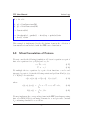
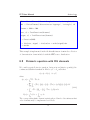
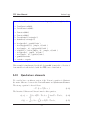
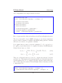
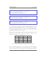


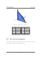
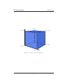

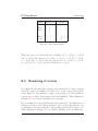
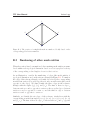

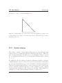
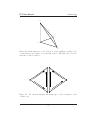

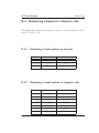
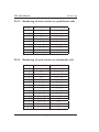




![arXiv:1208.4248v1 [math.AG] 21 Aug 2012](http://vs1.manualzilla.com/store/data/005698705_1-6d8998565962ce68b5a1333eba9cebce-150x150.png)