Download latest PDF - Read the Docs

SETLyze Documentation
Release 1.0.1
GiMaRIS
July 17, 2015
Contents
1
About SETLyze
2
Documentations
2.1 Installation . . . . . . . .
2.2 User Manual . . . . . . .
2.3 SETLyze Developer Guide
2.4 References . . . . . . . .
2.5 Legal Information . . . .
2.6 About Us . . . . . . . . .
3
1
.
.
.
.
.
.
.
.
.
.
.
.
.
.
.
.
.
.
.
.
.
.
.
.
.
.
.
.
.
.
.
.
.
.
.
.
.
.
.
.
.
.
.
.
.
.
.
.
.
.
.
.
.
.
.
.
.
.
.
.
.
.
.
.
.
.
.
.
.
.
.
.
.
.
.
.
.
.
.
.
.
.
.
.
.
.
.
.
.
.
.
.
.
.
.
.
.
.
.
.
.
.
.
.
.
.
.
.
.
.
.
.
.
.
.
.
.
.
.
.
.
.
.
.
.
.
.
.
.
.
.
.
.
.
.
.
.
.
.
.
.
.
.
.
.
.
.
.
.
.
.
.
.
.
.
.
.
.
.
.
.
.
.
.
.
.
.
.
.
.
.
.
.
.
.
.
.
.
.
.
.
.
.
.
.
.
.
.
.
.
.
.
.
.
.
.
.
.
.
.
.
.
.
.
.
.
.
.
.
.
.
.
.
.
.
.
.
.
.
.
.
.
.
.
.
.
.
.
.
.
.
.
.
.
.
.
.
.
.
.
3
3
4
30
60
60
61
Indices and tables
65
Python Module Index
67
i
ii
CHAPTER 1
About SETLyze
The purpose of SETLyze is to provide the people involved with the SETL project an easy and fast way of getting
useful information from the data stored in the SETL database. The SETL database at GiMaRIS contains data about
the settlement of species in Dutch waters. SETLyze helps provide more insight in a set of biological questions by
analyzing this data. SETLyze can perform the following set of analyses:
Spot Preference Determine a species’ preference for a specific location on a SETL plate. Species can be combined
so that they are treated as a single species.
Attraction within Species Determine if a species attracts or repels individuals of its own kind. Species can be combined so that they are treated as a single species.
Attraction between Species Determine if two different species attract or repel each other. Species can be combined
so that they are treated as a single species.
Additionally, any of the above analyses can be performed in batch mode, meaning that the analysis is repeated for each
species of a species selection. Thus an analysis can be easily performed on an entire data set without intervention.
Batch mode for analyses are parallelized such that the computing power of a computer is optimally used.
1
SETLyze Documentation, Release 1.0.1
2
Chapter 1. About SETLyze
CHAPTER 2
Documentations
2.1 Installation
2.1.1 Requirements
SETLyze runs on GNU/Linux, MacOS, and Microsoft Windows. The following software is required to run SETLyze:
• GTK+ (>=2.24.0,!=2.24.8,!=2.24.10)
• R
• Python (>=2.6 & <2.8)
– appdirs
– PyGTK, PyCairo, and PyGObject
– pandas
– RPy2
– xlrd (>=0.8)
Windows users can use the Windows installer for SETLyze, which installs all dependencies and creates shortcuts in
the Start menu and on the desktop.
On Debian (based) systems, the dependencies can be installed from the software repository:
sudo apt-get install python-appdirs python-gtk2 python-pandas python-rpy2 \
python-xlrd r-base-core
More recent versions of some Python packages can be obtained via the Python Package Index (preferably inside a
Python virtualenv):
pip install -r requirements.txt
Windows users should install the PyGTK all-in-one Windows installer. Then use pip as described above to install
the remaining dependencies. Note that this step is not needed if you have the Windows installer for SETLyze, which
comes bundeled with the requirements.
2.1.2 Installation
Windows users can use the Windows installer for SETLyze, which installs all dependencies and creates shortcuts in
the Start menu and on the desktop.
3
SETLyze Documentation, Release 1.0.1
If you want to install SETLyze from the GitHub repository:
git clone https://github.com/figure002/setlyze.git
pip install setlyze/
Or if you have a source archive file:
pip install setlyze-x.x.tar.gz
Once installed, the setlyze executable should be available.
2.1.3 Contributing
Please follow these steps to start working on the SETLyze code base:
1. Fork the project on github.com.
2. Create a new branch.
3. Commit changes to the new branch.
4. Send a pull request.
First make sure that all dependencies are installed as described above. Then follow the next steps to run and develop
SETLyze within a virtualenv isolated Python environment:
$ git clone https://github.com/figure002/setlyze.git
$ cd setlyze/
$ virtualenv --system-site-packages env
$ source env/bin/activate
(env)$ pip install -r requirements.txt
(env)$ python setup.py develop
(env)$ setlyze
2.2 User Manual
Welcome to the user manual for SETLyze. This manual explains the usage of SETLyze.
2.2.1 Introduction
SETLyze is a part of the SETL project, a fouling community study focussing on marine invasive species. The website
describes the SETL project as follows:
“Over the last ten years, marine invaders have had a dramatically increasing impact on temperate water
ecosystems around the world. Substantial ecological and economical damage has been caused by the
introduction of diseases, parasites, predators, invaders outcompeting native species, and species that are
a nuisance for public health, tourism, aquaculture or in any other way. In the SETL-project standardized
PVC-plates are used to detect these invasive species and other fouling community organisms. The material
and methods of the SETL-project were developed by the ANEMOON foundation in cooperation with the
Smithsonian Marine Invasions Laboratory of Smithsonian Environmental Research Centre. In this project
14x14 cm PVC-plates are hung 1 meter below the water surface, and refreshed and checked for species at
least every three months.” — ANEMOON foundation
Data collected from these SETL plates are stored in the SETL database. This database currently contains over 25000
records containing information of over 200 species in different locations throughout the Netherlands. SETLyze is an
application capable of performing a set of analyses on this SETL data. SETLyze can perform the following analyses:
4
Chapter 2. Documentations
SETLyze Documentation, Release 1.0.1
Spot Preference Determine a species’ preference for a specific location on a SETL plate. Species can be combined
so that they are treated as a single species.
Attraction within Species Determine if a species attracts or repels individuals of its own kind. Species can be combined so that they are treated as a single species.
Attraction between Species Determine if two different species attract or repel each other. Species can be combined
so that they are treated as a single species.
Additionally, any of the above analyses can be performed in batch mode, meaning that the analysis is repeated for each
species of a species selection. Thus an analysis can be easily performed on an entire data set without intervention.
Batch mode for analyses are parallelized such that the computing power of a computer is optimally used.
Data Collection
First let’s have a look at how the data for the SETL project is being collected. When the SETL plates are checked, each
plate is first carefully pulled out of the water and then photographed. This is done by a standard procedure described
on the ANEMOON foundation’s website. First an overview photograph is taken of each plate. Then some more
detailed photographs are taken of the species that grow on each plate. Indivdual plates are recognized by their tags.
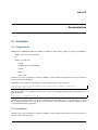
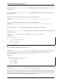
The pictures are then carefully analyzed. For each plate the SETL-monitoring form is filled in. For each species the
absence or presence, abundance and area cover are filled in. For this, a 5x5 grid is digitally applied over the photograph
(SETL plate with digitally applied grid). For each species the presence or absence on each of the 25 plate surfaces are
filled in and saved to the database.
Fig. 2.1: SETL plate with digitally applied grid
Each record in the database contains a species ID, a plate ID, and the 25 plate surfaces. The species ID links to the
species that was found on the plate. The plate ID links to the plate on which that species was found. The plate ID is
also linked to the location where this plate was deployed. The 25 plate surfaces (“spots”) are stored in each record as
booleans (meaning they can have a value of True or False). The value 1 (True) for a spot means that the species in
question was present on that spot of the plate. The value 0 (False) means that the species was absent from that spot.
With 25 spots x 2500 records = 625000+ booleans for the presence/absence of species, automatic methods of analyzing
this data are required. Hence SETLyze was developed, a tool for analyzing the settlement of species on SETL plates.
2.2.2 Using SETLyze
SETLyze comes with a graphical user interface (GUI). The GUI consists of dialogs which all have a specific task.
These dialogs will guide you in performing the set of analyses it provides. Most of SETLyze’s dialogs have a Help
button which when clicked should point you to the corresponding dialog description on this page. All dialog descriptions can be found in the SETLyze dialogs section of this manual.
Before SETLyze can perform an analysis it needs access to a data source containing SETL data. Currently two data
sources are supported: Text (.csv) or Excel (.xls) files exported from the Microsoft Access SETL database. This means
2.2. User Manual
5
SETLyze Documentation, Release 1.0.1
that the user must first export the tables of the SETL database from Microsoft Access to these files. This would result
in four files, one for each table. The user is then required to load these files into SETLyze. First follow the steps to
export the SETL data.
You can perform an analysis once you have loaded the four data files containing the SETL data. Start SETLyze and
you should be presented with the Analysis Selection dialog. Select an analysis and press OK to begin. A new dialog
will be displayed, most likely the Locations Selection dialog.
If this is your first time running SETLyze, the locations selection dialog will show an empty locations list because
no data has been loaded yet. To load SETL data, click on the Change Data Source button to open the change data
source dialog. This dialog allows you to load data from CSV or XLS files exported from the Microsoft Access SETL
database.
Once the data has been loaded, the locations selection dialog will automatically update the list of locations. From
here on it’s just a matter of following the instruction one the screen. Should you need more help, scroll down to the
SETLyze dialogs section for a more extensive description of each dialog. The dialog descriptions are also accessible
from SETLyze’s dialogs itself by clicking the Help button on a dialog.
Definition List
This part of the user manual describes some terminology often used throughout the application and this manual.
Intra specific Within a single species.
Inter specific Between two different species.
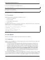
Plate area The defined area on a SETL plate. By default the SETL plate is divided in four plate areas (A, B, C and
D):
Fig. 2.2: Default plate areas
Plate areas can be customized during an analysis, see Define Plate Areas dialog.
Positive spot Each record in the SETL database contains data for each of the 25 spots on a SETL plate. The spots are
stored as booleans, meaning they can have two values; 1 (True) means that the species was present on that spot,
0 (False) means that the species was absent on that spot. A spot is “positive” if the spot value is 1 or True. Each
record can thus have up to 25 positive spots.
SETL plate In the SETL project standardized PVC-plates are used to detect invasive species and other fouling community organisms. In this project 14x14 cm PVC-plates are hung 1 meter below the water surface, and refreshed
and checked for species at least every three months.
6
Chapter 2. Documentations
SETLyze Documentation, Release 1.0.1
Spot To analyze SETL plates, photographs of the plates are taken. The photographs are then analyzed on the computer
by applying a 5x5 grid to the photographs. This divides the SETL plate into 25 equal surface areas (see SETL
plate with digitally applied grid). Each of the 25 surface areas are called “spots”. Species are scored for
presence/absence for each of the 25 spots on each SETL plate, and the data is stored in the SETL database in
the form of records. So each SETL record in the database contains presence/absence data of one species for all
25 spots on a SETL plate.
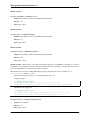
Spot distance Spot distances are the distances between positive spots on a SETL plate. The spot distances are calculated from observed and expected positive spots data and are used to define whether species attract or repel.
Observed spot distances (intra specific)
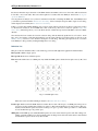
All possible distances between the spots on each plate are calculated using the Pythagorean theorem. Consider
the case of species A and the following plate:
Fig. 2.3: Spot distances on SETL plate (intra specific)
As you can see from the figure, three positive spots results in three spot distances (a, b and c). The distance
from one spot to the next by moving horizontally or vertically is defined as 1. The distances from the figure are
calculated as follows:
√
𝑠𝑝𝑜𝑡_𝑑𝑖𝑠𝑡𝑎𝑛𝑐𝑒(𝑎) = 32 + 22 = 3.61
√
𝑠𝑝𝑜𝑡_𝑑𝑖𝑠𝑡𝑎𝑛𝑐𝑒(𝑏) = 32 + 12 = 3.16
√
𝑠𝑝𝑜𝑡_𝑑𝑖𝑠𝑡𝑎𝑛𝑐𝑒(𝑐) = 02 + 32 = 3
This is done for all plates of an analysis. Note that there can be no distance 0, in contrast to inter specific spot
distances (see below).
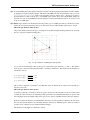
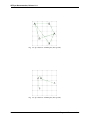
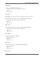
Observed spot distances (inter specific)
To obtain spot distances for analyses where two species are involved, first the plate records are collected that
contain both of the selected species. Then all possible spot distances are calculated between the two species. The
following figure shows an example with positive spots for two species (A and B) and all possible spot distnaces.
In the above figure, the distances are calculated the same way as for intra specific spot distances. Note however
that only inter specific distances are calculated (distances between two different species). This also makes it
possible to have a distance of 0 as visualized in the next figure.
The distances for this figure are calculated as follows:
2.2. User Manual
7
SETLyze Documentation, Release 1.0.1
Fig. 2.4: Spot distances on SETL plate (inter specific)
Fig. 2.5: Spot distances on SETL plate (inter specific)
8
Chapter 2. Documentations
SETLyze Documentation, Release 1.0.1
√
𝑠𝑝𝑜𝑡_𝑑𝑖𝑠𝑡𝑎𝑛𝑐𝑒(𝑎) = 02 + 02 = 0
√
𝑠𝑝𝑜𝑡_𝑑𝑖𝑠𝑡𝑎𝑛𝑐𝑒(𝑏) = 32 + 12 = 3.16
√
𝑠𝑝𝑜𝑡_𝑑𝑖𝑠𝑡𝑎𝑛𝑐𝑒(𝑐) = 02 + 22 = 2
Expected spot distances
The expected spot distances are calculated by generating a copy of each plate record matching the species
selection. Each copy has the same number of positive spots as its original, except the positive spots are placed
randomly at the plates. Then the spot distances are calculated the same way as for the observed spot distances.
This means that the resulting list of expected spot distances has the same length as the observed spot distances.
2.2.3 SETLyze dialogs
SETLyze comes with a graphical user interface consisting of separate dialogs. The dialogs are described in this section.
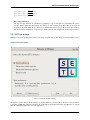
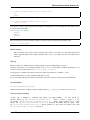
Analysis Selection dialog
Fig. 2.6: Analysis Selection dialog
The analysis selection dialog is the first dialog you see when SETLyze is started. It allows the user to select an analysis
to perform on SETL data. The user can select one of the analyses in the list and click on the OK button to start the
analysis. Clicking the Quit button closes the application.
2.2. User Manual
9
SETLyze Documentation, Release 1.0.1
After pressing the OK button, two things can happen. If no SETL data was found on the user’s computer, SETLyze
automatically tries to load SETL locations and species data from the SETL database server. This requires a direct
connection with the SETL database server. A progress dialog is shown while the data is being loaded. If connecting
to the database server fails, SETLyze continues without data. Since the database server has not been implemented yet,
no data will be loaded.
If SETL data is found on the user’s computer, an information dialog is displayed telling the user that existing data is
being loaded.
Clicking the About button shows SETLyze’s About dialog. The About dialog shows general information about SETLyze; its version number, license information, a link to the GiMaRIS website, the application developers, and contact
information.
Clicking the Preferences button loads the Preferences dialog.
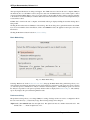
Batch Mode dialog
Fig. 2.7: Batch Mode dialog
Selecting “Batch mode” in the Analysis Selection dialog brings up the Batch Mode dialog. This dialog allows you to
start an analysis in batch mode. In batch mode, the selected analysis is repeated for each species in a species selection
(or each inter species combination for analysis “Attraction between Species”). When multiple species are selected
the analysis is repeated for each species separately and the results are displayed in a Summary Report. The summary
report only displays the species that had significant results.
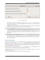
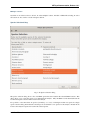
Preferences dialog
The preferences dialog allows you to change SETLyze’s settings. Settings set here are saved to a configuration file in
the user’s home directory (~/.setlyze/setlyze.cfg). The following settings can be changed:
Alpha level (𝛼) for statistical tests Sets the alpha level. The alpha level must be a number between 0 and 1. The
default value 0.05 means an alpha level of 5%.
10
Chapter 2. Documentations
SETLyze Documentation, Release 1.0.1
Fig. 2.8: Preferences dialog
This alpha level is translated to a confidence level with the formula 𝑐𝑜𝑛𝑓.𝑙𝑒𝑣𝑒𝑙 = 1 − 𝛼. This confidence level
is used for some statistical tests to calculate the confidence interval. At this moment this is just the t-test (not
used in any analysis at this point).
The alpha level is also used to determine if a P-value returned by statistical tests is considered significant. The
P-value is considered significant if the P-value is equal or less than the alpha level.
Number of repeats for statistical tests Sets the number of repeats to perform on some statistical tests. Some statistical tests used in SETLyze use expected values that are randomly generated. This means you can’t draw a solid
conclusion from the result of just one test. There is a change that the found result was a coincidence. To account
for this, these test are repeated a number of times. The default value is 20 repeats. This value is very low, but
good enough for testing purposes. When you need to draw solid conclusions, this value needs to be set to a
higher number.
Number of concurrent processes for batch mode Batch mode for analyses are parallelized which means that multiple analyzes can be executed in parallel. The value set here corresponds to the number of concurrent processes
that will execute analyses. The higher the number, the faster a batch analysis will complete. The number of
processes must be at least 1 and no more than the number of CPUs. The default value of this option equals to
90% of the available CPUs.
Locations Selection dialog
The locations selection dialog shows a list of all SETL locations. This dialog allows you to select locations from
which you want to select species. The Species Selection dialog (displayed after clicking the Continue button) will only
display the species that were recorded in the selected locations. Subsequently this means that only the SETL records
that match both the locations and species selection will be used for the analysis, as each SETL record is bound to a
species and a SETL plate from a specific location.
The Change Data Source button opens the Load Data dialog. This dialog allows you to load new SETL data. After
doing so, the locations selection dialog is automatically updated with the new data.
The Back button allows you to go back to the previous dialog. This can be useful when you want to correct a choice
you made in a previous dialog.
The Continue button saves the selection, closes the dialog, and shows the next dialog.
2.2. User Manual
11
SETLyze Documentation, Release 1.0.1
Fig. 2.9: Locations Selection dialog
12
Chapter 2. Documentations
SETLyze Documentation, Release 1.0.1
Making a selection
Just click on one of the locations to select it. To select multiple locations, hold Ctrl or Shift while selecting. To select
all locations at once, click on a location and press Ctrl+A.
Species Selection dialog
Fig. 2.10: Species Selection dialog
The species selection dialog shows a list of all SETL species that were found in the selected SETL locations. This
dialog allows you to select the species to be included in the analysis. Only the SETL records that match both the
locations and species selection will be used for the analysis.
It is possible to select more than one species (see Making a selection). Selecting more than one species in a single
species selection dialog means that the selected species are threated as one species for the analysis. In batch mode
however, the analysis is repeated for each of the selected species.
2.2. User Manual
13
SETLyze Documentation, Release 1.0.1
If the selected analysis requires two or more separate species selections (e.g. two species are compared), it will display
the selection dialog multiple times. In this case, the header of the selection dialog will say “First Species Selection”,
“Second Species Selection”, etc.
The Back button allows you to go back to the previous dialog. This can be useful when you want to correct a choice
you made in a previous dialog.
The Continue button saves the selection, closes the dialog, and shows the next dialog.
Making a selection
Just click on one of the species to select it. To select multiple species, hold Ctrl or Shift while selecting. To select all
species at once, click on a species and press Ctrl+A.
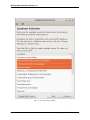
Load Data dialog
Fig. 2.11: Load Data dialog
The Load Data dialog allows you to load SETL data into SETLyze. Two data sources are supported:
14
Chapter 2. Documentations
SETLyze Documentation, Release 1.0.1
• Text CSV (*.csv, *.txt) files exported from the Microsoft Access SETL database. The CSV files need to be exported by Microsoft Access, one file for each of the four tables: SETL_localities, SETL_plates, SETL_records,
and SETL_species. The section Exporting SETL data from the Access database describes how to export these
files.
• Excel 97/2000/XP/2003 (*.xls) files exported from the Microsoft Access SETL database. One file for each
of the four tables: SETL_localities, SETL_plates, SETL_records, and SETL_species. Microsoft Access by
default includes a header row in the exported XLS files. The header row must be removed before importing into
SETLyze.
After selecting all four data files files, press the OK button to load the SETL data from these files. A progress dialog is
shown while the data is being loaded. Once the data has been loaded, the Locations Selection dialog will be updated
with the new data.
Define Plate Areas dialog
This dialog allows you to define the plate areas for analysis “Spot Preference”. By default, the SETL plate is divided
in four plate areas: A, B, C and D. This dialog allows you to combine these areas by changing the area definitions.
Combining areas means that the combined areas are treated as a single plate area. One must define at least two plate
areas.
The user defined plate areas are only used for the Chi-squared test. In any case the Wilcoxon test will analyze the plate
areas A, B, C, D, A+B, C+D, A+B+C and B+C+D.
Below is a schematic SETL plate with a grid. By default the plate is divided in four plate areas (A, B, C and D),
But sometimes it’s useful to combine plate areas. So if one decides to combine areas A and B, the selection could be
changed as follows,
And the resulting plate areas definition would look something like this,
This would result in three plate areas. Analysis “Spot Preference” would then determine if the selected species has a
preference for either of the three plate areas.
The names of the plate areas (area 1, area 2, ...) do not have a special meaning. It is simply used internally by the
application to distinguish between plate areas. These area names are also used in the analysis report to distinguish
between the plate areas.
The Back button allows you to go back to the previous dialog. This can be useful when you want to correct a choice
you made in a previous dialog.
The Continue button saves the selection, closes the dialog, and shows the next dialog.
Analysis Report dialog
The analysis report dialog shows the results for an analysis. The dialog consists of the results frame and a toolbar
on top. The toolbar holds a number of buttons. Hover your mouse pointer over the buttons to reveal a tooltip which
explains the button’s action. Some buttons are explained below:
Save The “Save” button allows you to save the report to a file. Clicking this button first shows a File Save dialog
which allows you to select a target directory and filename. One file type is supported:
• reStructuredText (*.rst) - Plain text files in an easy-to-read markup syntax. One can use Docutils to convert
reStructuredText files into useful formats, such as HTML, LaTeX, man-pages, open-document or XML.
Save All The “Save All” button is only enabled in batch mode and allows you to export the reports of the individual
analyses. Clicking the “Save” button in batch mode only saves the Summary Report which is based on the
individual reports.
2.2. User Manual
15
SETLyze Documentation, Release 1.0.1
Fig. 2.12: Define Plate Areas dialog
16
Chapter 2. Documentations
SETLyze Documentation, Release 1.0.1
Fig. 2.13: Default plate areas
Fig. 2.14: Combined plate areas selection
2.2. User Manual
17
SETLyze Documentation, Release 1.0.1
Fig. 2.15: Plate areas A and B combined.
Fig. 2.16: Analysis Report dialog
18
Chapter 2. Documentations
SETLyze Documentation, Release 1.0.1
Repeat The “Repeat” button can be used to repeat an analysis with different parameters. Clicking this button will
open a dialog which shows the same parameters available in the Preferences dialog. So one can, for example,
quickly repeat the analysis with a different number of repeats.
The report dialog can display two types of reports:
• Standard Report: When running an analysis in standard mode (not in batch mode) the report is divided into
sections. There is a section for each statistical test that was performed.
• Summary Report: When running an analysis in batch mode the report will be a summary of all standard reports
that were generated. This report will show less details than a standard report.
Both types of reports will be explained below.
Standard Report
A standard report is divided into subsections. You have to click on a subsection to reveal its contents. Find the
explanation for each subsection below.
Locations and Species Selections Displays the locations and species selections. If multiple selections were made,
each element is suffixed by a number. For example “Species selection (2)” stands for the second species selection.
Wilcoxon rank sum test with continuity correction Shows the results for the non-repeated Wilcoxon rank-sum
tests.
“In statistics, the Mann–Whitney U test (also called the Mann–Whitney–Wilcoxon (MWW) or Wilcoxon
rank-sum test) is a non-parametric statistical hypothesis test for assessing whether two independent samples of observations have equally large values.” — Mann–Whitney U (Wikipedia. 6 December 2010)
Tests showed that spot distances on a SETL plate are not normally distributed (see Testing spot distances for normal
distribution), hence the Wilcoxon rank-sum test for unpaired data was chosen to test if observed and expected spot
distances differ significantly. The observed and expected spot distances
Depending on the analysis, the test is performed on different groups of data. The data can be grouped by plate area
(analysis “Spot Preference”), the number of positive spots (analysis “Attraction within Species”) or by positive spot
ratios groups (analysis “Attraction between Species”). See section record grouping for more information on data
grouping.
Each row for the results of the Wicoxon test contains the results of a single test on a data group. Each row can have
the following elements:
Plate Area The plate area of a SETL plate. A SETL plate is divided into four plate areas: A, B, C, and D (see Default
plate areas). The test is performed on each of the four plate areas, plus the combinations “A+B”, “C+D”,
“A+B+C”, and “B+C+D”. Combining the results of the test for all plate areas (and combinations) allows you to
make conclusions about the species’ preference for areas on SETL plates. See also Grouping by Plate Area.
Positive Spots A number representing the number of positive spots. For this test only records matching that number
of positive spots were used. See also Record grouping by number of positive spots.
Ratios Group A number representing the ratios group. For this test only records grouped in that ratios group were
used. See also Record grouping by ratios groups.
n (totals) The number of values (n) used for the statistical test. Each value (x) is a number representing the number
of encounters of a species on a plate area for a specific record in the database. So a value x=4 means that the
species was found on four spots of the area in question for a specific plate. If the area in question was “A”,
then the maximum value for x would be 4, because area “A” consists of four spots. This is done for all records
matching that species and plate area, resulting in a sequence of numbers (e.g. 1,0,0,3,12,4,8,0,...).
So n is the number of values x.
2.2. User Manual
19
SETLyze Documentation, Release 1.0.1
n (observed species) The number of times the species was found on the plate area in question. This is for all plates
summed up.
n (expected species) The number of times you’d expect the species to be found on the plate area in question. The
expected values are calculated per plate with a random generator. For each plate, the same number of positive
spots are generated randomly on a virtual plate. The number of positive spots are then counted for the plate area
in question.
n (plates) The number of plates that match the number of positive spots.
n (distances) The number of spot distances derived from the records matching the positive spots number.
P-value The P-value for the test.
Mean Observed The mean of the observed spot distances. This is calculated separately.
Mean Expected The mean of the expected spot distances. This is calculated separately.
Remarks A summary of the results. Shows whether the p-value is significant (p-value <= alpha level), and if so, how
significant and decides based on the means if the species attract species/reject a plate area (observed mean <
expected mean) or repel species/prefer a plate area (observed mean > expected mean).
Some data groups might me missing from the list of results. This is because groups that don’t have matching records
are skipped, so they are not displayed in the list of results.
Wilcoxon rank sum test with continuity correction (repeated) Shows the significance results for the repeated
Wilcoxon tests. For more information about the Wilcoxon rank-sum test results, see Wilcoxon rank sum test with
continuity correction.
The number of repeats to perform can be set in the Preferences dialog.
Each row for the results of the repeated Wicoxon test contains the results of repeated tests on a data group. Each row
can have the following elements:
Plate Area See description for Wilcoxon rank sum test with continuity correction.
n (totals) See description for Wilcoxon rank sum test with continuity correction.
n (observed species) See description for Wilcoxon rank sum test with continuity correction.
n (significant) Shows how many times the test turned out significant for the repeats (P-value <= alpha level).
n (non-significant) Shows how many times the test turned out to be not significant for the repeats (P-value > alpha
level).
n (preference) Shows how many times there was a significant preference for the plate area in question.
n (rejection) Shows how many times there was a significant rejection for the plate area in question.
n (attraction) Shows how many times there was a significant attraction for the species in question.
n (repulsion) Shows how many times there was a significant repulsion for the species in question.
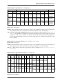
Chi-squared test for given probabilities Shows the results for Pearson’s Chi-squared Test for Count Data.
“Pearson’s chi-square (𝜒2) test is the best-known of several chi-square tests. It tests a null hypothesis
stating that the frequency distribution of certain events observed in a sample is consistent with a particular
theoretical distribution.” — Pearson’s Chi-squared Test (Wikipedia. 23 December 2010)
The observed values are the frequencies of the observed spot distances. The expected values are calculated with the
formula 𝑒(𝑑) = 𝑁 * 𝑝(𝑑) where N is the total number of observed distances and p is the probability for spot distance
d. The probability p has been pre-calculated for each spot distance. The probabilities for intra-specific spot distances
are from the model of Distribution for intra-specific spot distances and the probabilities for inter-specific distances
20
Chapter 2. Documentations
SETLyze Documentation, Release 1.0.1
are from the model of Distribution for inter-specific spot distances. The probabilities have been hard coded into the
application:
Intra-specific spot distances:
Spot Distance
1
1.41
2
2.24
2.83
3
3.16
3.61
4
4.12
4.24
4.47
5
5.66
Probability
40/300
32/300
30/300
48/300
18/300
20/300
32/300
24/300
10/300
16/300
8/300
12/300
8/300
2/300
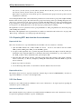
Inter-specific spot distances:
Spot Distance
0
1
1.41
2
2.24
2.83
3
3.16
3.61
4
4.12
4.24
4.47
5
5.66
Probability
25/625
80/625
64/625
60/625
96/625
36/625
40/625
64/625
48/625
20/625
32/625
16/625
24/625
16/625
4/625
Depending on the analysis, the records matching the species selection are first grouped by positive spots number
(analysis “Attraction within Species”) or by ratios group (analysis “Attraction between Species”). See section Record
Grouping.
Each row for the results of the Chi-squared tests contains the results of a single test on a spots/ratios group. Each row
can have the following elements:
Positive Spots A number representing the number of positive spots. For this test only records matching that number
of positive spots were used.
Ratios Group A number representing the ratios group. For this test only records grouped in that ratios group were
used.
n (plates) The number of plates that match the number of positive spots.
n (distances) The number of spot distances derived from the records matching the positive spots number.
P-value The P-value for the test.
2.2. User Manual
21
SETLyze Documentation, Release 1.0.1
Chi squared The value the Chi-squared test statistic.
df The degrees of freedom of the approximate chi-squared distribution of the test statistic.
Mean Observed The mean of the observed spot distances. This is calculated separately.
Mean Expected The mean of the expected spot distances. This is calculated separately.
Remarks A summary of the results. Shows whether the p-value is significant, and if so, how significant and decides
based on the means if the species attract (observed mean < expected mean) or repel (observed mean > expected
mean).
Some spots/ratios groups might me missing from the list of results. This is because spots/ratios groups that don’t have
matching records are skipped, so they are not displayed in the list of results.
Plate Areas Definition for Chi-squared Test Describes the definition of the plate areas set with the Define Plate
Areas dialog. See the description for that dialog to get the meaning of the letters A, B, C and D.
Species Totals per Plate Area for Chi-squared Test
Area ID See the Plate Areas Definition for Chi-squared Test section of the report to see the definition of each area.
Observed Totals How many times the selected species was found present in each of the plate areas.
Expected Totals The expected totals for the selected species.
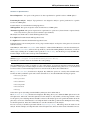
Summary Report
A summary report contains basic information from multiple standard reports. Such a summary report is basically a
table where each row represents a single analysis and the columns contain the results per data group.
In the summary report a result is only displayed if one of the statistical tests done for a species (combination) was
considered significant. Some statistical tests are repeated and in this case there is a p-value for each repeat. In this
case the p-value is calculated with 𝑝 = 1 − (𝑠/𝑡) where s is the number of significant p-values for the major form
of significance. For example, if attraction was more often significant than rejection, then s is the total number of
significant p-values for attraction. And t is the total number of repeats for the test. So with 20 repeats and 𝛼 = 0.05,
19 out of 20 repeats must have had a significant p-value in one direction for the test result to be considered significant.
Below are the definitions for the result codes used in summary reports.
na There is not enough data for the analysis or in case of the Chi Squared test one of the expected frequencies is less
than 5.
s The result for the statistical test was significant.
ns The result for the statistical test was not significant.
pr There was a significant preference for the plate area in question.
rj There was a significant rejection for the plate area in question.
at There was a significant attraction for the species in question.
rp There was a significant repulsion for the species in question.
The summary report for each analysis are explained below.
22
Chapter 2. Documentations
SETLyze Documentation, Release 1.0.1
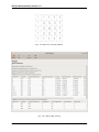
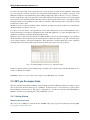
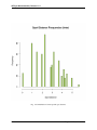
Summary Report “Spot Preference” Example report:
Species
Obelia
dichotoma
Obelia
geniculata
Obelia
longissima
Wilcoxon rank sum test
A
B
C
Chi-sq
A+B+C B+C+D A,B,C,D
n
D
A+B
C+D
(plates)
177
pr;
ns;
rj;
ns;
ns;
rj;
ns;
ns;
s;
p=0.0000 p=1.0000 p=0.0000 p=0.0500 p=0.3500 p=0.0000 p=1.0000 p=1.0000 𝜒²=103.98;
p=0.0000
91
ns;
ns;
rj;
ns;
ns;
rj;
ns;
ns;
s; 𝜒²=62.30;
p=0.4500 p=1.0000 p=0.0000 p=0.1000 p=1.0000 p=0.0000 p=1.0000 p=1.0000 p=0.0000
341
pr;
ns;
rj;
rj;
pr;
rj;
ns;
rj;
s;
p=0.0000 p=1.0000 p=0.0000 p=0.0000 p=0.0000 p=0.0000 p=1.0000 p=0.0000 𝜒²=435.22;
p=0.0000
Explanation of the columns:
Species Name of the species.
n (plates) The total number of plates for the species selection. The real number of plates used for each data group
may be smaller. Use the “Save All” button to see the number of plates used for each data group.
A, B, C, D, A+B, C+D, A+B+C, and B+C+D In this report the results are grouped by plate area (see Grouping by
Plate Area). For the Wilcoxon rank sum test, the test is performed on each of the four plate areas, plus the
combinations “A+B”, “C+D”, “A+B+C”, and “B+C+D”. For the Chi squared test the user defined plate areas
are used. The user defined plate areas can be seen in the column name (e.g. “A+B,C,D” means that areas A and
B were combined).
Summary Report “Attraction within Species” Explanation of the columns:
Species Name of the species.
n (plates) The total number of plates for the species selection. The real number of plates used for each data group
may be smaller. Use the “Save All” button to see the number of plates used for each data group.
2-24, 2, 3, ..., 24 In this report the results are grouped by positive spot numbers (see Record grouping by number of
positive spots).
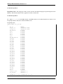
Summary Report “Attraction between Species” Example report:
Wilcoxon rank sum test
Chi-squared test
SpeciesSpeciesn
11
2
3
4
5
1-5
1
2
3
4
5
A
B
(plates)
5
Obelia Obelia 12 ns; ns; at;
ns; na
na
ns;
rp;
at;
ns;
na
na
digenicp=0.8500
p=0.0500
p=0.0000
p=1.0000
𝜒²=16.90;𝜒²=35.36;𝜒²=38.12;𝜒²=7.21;
chotomaup=0.2615p=0.0013p=0.0005p=0.9263
lata
Obelia Obelia 81 rp; ns; rp; rp; rp; rp; rp;
rp;
rp;
rp;
rp;
rp;
dilongisp=0.0000
p=0.1000
p=0.0000
p=0.0000
p=0.0000
p=0.0000
𝜒²=420.68;
𝜒²=134.34;
𝜒²=164.86;
𝜒²=170.01;
𝜒²=96.88;𝜒²=43.53;
chotomasima
p=0.0000p=0.0000p=0.0000p=0.0000p=0.0000p=0.0001
Obelia Obelia 39 rp; ns; ns; ns; ns; rp; rp;
rp;
rp;
rp;
ns;
rp;
genic- longisp=0.0000
p=0.9500
p=0.9500
p=0.5500
p=0.9500
p=0.0000
𝜒²=211.92;
𝜒²=39.46;𝜒²=28.69;𝜒²=105.26;
𝜒²=8.14; 𝜒²=141.94;
usima
p=0.0000p=0.0003p=0.0115p=0.0000p=0.8821p=0.0000
lata
In this example the columns containing numbers (1,2,..) represent
Explanation of the columns:
2.2. User Manual
23
SETLyze Documentation, Release 1.0.1
Species A Name of the first species.
Species B Name of the species the first species was compared with.
n (plates) The total number of plates for the species selection. The real number of plates used for each data group
may be smaller. Use the “Save All” button to see the number of plates used for each data group.
1-5, 1, 2, 3, 4, 5 In this report the results are grouped by positive spot ratio groups (see Record grouping by ratios
groups).
Record Grouping
SETLyze performs statistical tests to determine the significance of results. The key statistical tests used to determine
significance are the Wilcoxon rank-sum test and Pearson’s Chi-squared test. The tests are performed on records data
that match the locations and species selection. It is however not a good idea to just perform the test on all matching
records. For this reason the matching records are first grouped by a specific property. The tests are then performed on
each group.
Two methods for grouping records have been implemented. One is by positive spots number, and the other is by
positive spots ratio. We’ll describe each grouping method below.
Grouping by Plate Area
This type of grouping is done for analysis “Spot Preference”. Each group is a plate area or a combination of plate
areas. The following groups are defined:
1. Plate area A
2. Plate area B
3. Plate area C
4. Plate area D
5. Plate area A+B
6. Plate area B+C
7. Plate area A+B+C
8. Plate area B+C+D
For each group, the number of positive spots for all plates and that specific plate area are calculated. These make up
the observed values.
Record grouping by number of positive spots
This type of grouping is done in the case of calculated spot distances for a single species (or multiple species grouped
together) on SETL plates (analysis “Attraction within Species”).
A record has a maximum of 25 positive spots, so this results in a maximum of 25 record groups. Group 1 contains
records with just one positive spot, group 2 contains records with two positive spots, et cetera. Records of group 1
and 25 are left out however. Group 1 is skipped because it is not possible to calculate spot distances for records with
just one positive spot. And group 25 is excluded because a significance test on records of this group will always result
in a p-value of 1. This makes sense, because both the observed and expected distances are based on records with 25
positive spots, which is a full SETL plate. As a result, the observed and expected spot distances will be exactly the
same.
24
Chapter 2. Documentations
SETLyze Documentation, Release 1.0.1
The test is also performed on a group with number -24. Of course there is no such thing as records with minus 24
positive spots. Actually, the minus sign should be read as “up to”. So this test is also performed on records with up to
24 positive spots. This means that the significance test will also be performed on records of all groups together. Note
that records of group 1 will still be ignored.
The results of the significance tests are presented in rows. Each row contains the result of the test for one group. The
“Positive Spots” column tells you to which group each result belongs.
Record grouping by ratios groups
This type of grouping is done in the case of calculated spot distances between two different (groups of) species
(analysis “Attraction between Species”).
When dealing with two species, plate records are matched that contain both species. This means we can get a ratio for
the positive spots for each matching SETL plate record. Consider Spot distances on SETL plate (inter specific) which
visualizes a SETL plate with positive spots of species A and B. There are two positive spots of one species, and three
positive spots of the other. That makes the ratio for this plate 2:3. The order of the species doesn’t matter here, so a
ratio A:B is considered the same as ratio B:A. All records are grouped based on this ratio. We’ve defined five ratios
groups:
Note:
𝑐 = 𝑐𝑜𝑚𝑏(𝑠) A function for generating a list of two-item combinations with replacement c from a sequence of numbers s. The two-item combinations are ratios (e.g. (2,3) = ratio 2:3).
𝑠 = 𝑠𝑒𝑞(𝑠𝑡𝑎𝑟𝑡, 𝑒𝑛𝑑) A function for creating a sequence of numbers s from a number range starting with start and
ending at end. For example 𝑠𝑒𝑞(1, 6) = 1, 2, 3, 4, 5
Ratios group 1: 𝑐𝑜𝑚𝑏(𝑠𝑒𝑞(1, 6)) = (1, 1), (1, 2), (1, 3), (1, 4), (1, 5), (2, 2), (2, 3), (2, 4), (2, 5), (3, 3), (3, 4), (3, 5),
(4, 4), (4, 5), (5, 5)
Ratios group 2: 𝑐𝑜𝑚𝑏(𝑠𝑒𝑞(1, 11)) − 𝑐𝑜𝑚𝑏(𝑠𝑒𝑞(1, 6)) = (1, 6), (1, 7), (1, 8), (1, 9), (1, 10), (2, 6), (2, 7), (2, 8), (2,
9), (2, 10), (3, 6), (3, 7), (3, 8), (3, 9), (3, 10), (4, 6), (4, 7), (4, 8), (4, 9), (4, 10), (5, 6), (5, 7), (5, 8), (5, 9), (5,
10), (6, 6), (6, 7), (6, 8), (6, 9), (6, 10), (7, 7), (7, 8), (7, 9), (7, 10), (8, 8), (8, 9), (8, 10), (9, 9), (9, 10), (10, 10)
Ratios group 3: 𝑐𝑜𝑚𝑏(𝑠𝑒𝑞(1, 16)) − 𝑐𝑜𝑚𝑏(𝑠𝑒𝑞(1, 11)) = (1, 11), (1, 12), (1, 13), (1, 14), (1, 15), (2, 11), (2, 12), (2,
13), (2, 14), (2, 15), (3, 11), (3, 12), (3, 13), (3, 14), (3, 15), (4, 11), (4, 12), (4, 13), (4, 14), (4, 15), (5, 11), (5,
12), (5, 13), (5, 14), (5, 15), (6, 11), (6, 12), (6, 13), (6, 14), (6, 15), (7, 11), (7, 12), (7, 13), (7, 14), (7, 15), (8,
11), (8, 12), (8, 13), (8, 14), (8, 15), (9, 11), (9, 12), (9, 13), (9, 14), (9, 15), (10, 11), (10, 12), (10, 13), (10, 14),
(10, 15), (11, 11), (11, 12), (11, 13), (11, 14), (11, 15), (12, 12), (12, 13), (12, 14), (12, 15), (13, 13), (13, 14),
(13, 15), (14, 14), (14, 15), (15, 15)
Ratios group 4: 𝑐𝑜𝑚𝑏(𝑠𝑒𝑞(1, 21)) − 𝑐𝑜𝑚𝑏(𝑠𝑒𝑞(1, 16)) = (1, 16), (1, 17), (1, 18), (1, 19), (1, 20), (2, 16), (2, 17), (2,
18), (2, 19), (2, 20), (3, 16), (3, 17), (3, 18), (3, 19), (3, 20), (4, 16), (4, 17), (4, 18), (4, 19), (4, 20), (5, 16), (5,
17), (5, 18), (5, 19), (5, 20), (6, 16), (6, 17), (6, 18), (6, 19), (6, 20), (7, 16), (7, 17), (7, 18), (7, 19), (7, 20), (8,
16), (8, 17), (8, 18), (8, 19), (8, 20), (9, 16), (9, 17), (9, 18), (9, 19), (9, 20), (10, 16), (10, 17), (10, 18), (10, 19),
(10, 20), (11, 16), (11, 17), (11, 18), (11, 19), (11, 20), (12, 16), (12, 17), (12, 18), (12, 19), (12, 20), (13, 16),
(13, 17), (13, 18), (13, 19), (13, 20), (14, 16), (14, 17), (14, 18), (14, 19), (14, 20), (15, 16), (15, 17), (15, 18),
(15, 19), (15, 20), (16, 16), (16, 17), (16, 18), (16, 19), (16, 20), (17, 17), (17, 18), (17, 19), (17, 20), (18, 18),
(18, 19), (18, 20), (19, 19), (19, 20), (20, 20)
Ratios group 5: 𝑐𝑜𝑚𝑏(𝑠𝑒𝑞(1, 25)) − 𝑐𝑜𝑚𝑏(𝑠𝑒𝑞(1, 21)) = (1, 21), (1, 22), (1, 23), (1, 24), (2, 21), (2, 22), (2, 23), (2,
24), (3, 21), (3, 22), (3, 23), (3, 24), (4, 21), (4, 22), (4, 23), (4, 24), (5, 21), (5, 22), (5, 23), (5, 24), (6, 21), (6,
22), (6, 23), (6, 24), (7, 21), (7, 22), (7, 23), (7, 24), (8, 21), (8, 22), (8, 23), (8, 24), (9, 21), (9, 22), (9, 23), (9,
24), (10, 21), (10, 22), (10, 23), (10, 24), (11, 21), (11, 22), (11, 23), (11, 24), (12, 21), (12, 22), (12, 23), (12,
24), (13, 21), (13, 22), (13, 23), (13, 24), (14, 21), (14, 22), (14, 23), (14, 24), (15, 21), (15, 22), (15, 23), (15,
24), (16, 21), (16, 22), (16, 23), (16, 24), (17, 21), (17, 22), (17, 23), (17, 24), (18, 21), (18, 22), (18, 23), (18,
2.2. User Manual
25
SETLyze Documentation, Release 1.0.1
24), (19, 21), (19, 22), (19, 23), (19, 24), (20, 21), (20, 22), (20, 23), (20, 24), (21, 21), (21, 22), (21, 23), (21,
24), (22, 22), (22, 23), (22, 24), (23, 23), (23, 24), (24, 24)
Ratios where one species has covered all 25 spots are excluded from this group because the p-value would be
insignificant for such ratios.
You can imagine that the results of the statistical test performed on records from ratios group 1 has a higher reliability
than the results for ratios group 5. Records from ratios group 1 have fewer positive spots. Finding that species A is
often close to species B on records of group 5 doesn’t say much. The high number of positive spots naturally results
in spots sitting close to each other. This is however not the case for records of group 1, where there is enough space
for the species to sit. Finding them next to each other in group 1 probably means something.
The significance test is also performed on ratios group with number -5. This group includes ratios from all 5 groups
(still excluding ratios with 25).
The results of the significance tests are presented in rows. Each row contains the result of the test for one group. The
“Ratios Group” column tells you to which group each result belongs.
2.2.4 Exporting SETL data from the Access database
Export to CSV files
This section describes how to export the SETL data from the Microsoft Access database to CSV files.
1. Open the SETL database file (*.mdb) in Microsoft Access. You’ll see four tables in the left column:
SETL_localities, SETL_plates, SETL_records and SETL_species.
2. To export a table, right-click on it to open the drop menu. From the menu select Export > Text file. Then give
the filename of the output file. Make sure to include the table name in the filename (e.g. setl_localities.csv for
the “SETL_localities” table). Uncheck all other options and press OK.
3. In the next dialog that appears select the option that separates fields with a character. The separator character
must be a semicolon (”;”). If it’s not, change it by clicking the Advanced button. Then click Finish to export the
data to a CSV file.
4. Repeat steps 2 and 3 for all tables.
5. You should end up with four files, one CSV file for each table. Put these files in one folder.
Export to Excel files
The database tables can also be exported to Excel files. Only the import of Excel 97/2000/XP/2003 (*.xls) files are
supported by SETLyze, so be sure to select the right format.
2.2.5 Use Cases
Possible use cases which describe how SETLyze can be used to find answers to biological questions regarding the
settlement of species on SETL plates.
Use Cases for SETLyze
This document describes some possible use cases which describe how SETLyze can be used to find answers to biological questions regarding the settlement of species on SETL-plates.
26
Chapter 2. Documentations
SETLyze Documentation, Release 1.0.1
Use Case 1: Spot Preference
Research Question “Do species of the genus Obelia have a preference for specific locations on SETL-plates?”
Performing the analysis Analysis “Spot preference” was designed to analyse a species’ preference for a specific
location on a SETL-plates.
For this analysis, we can define the following hypotheses:
Null hypothesis The species in question settles at random areas of SETL-plates.
Alternative hypothesis The species in question has a preference for a plate area (observed mean > expected mean)
or has a rejection for a plate area (observed mean < expected mean).
The analysis uses the P-value to decide which hypothesis is true.
P >= alpha level Assume that the null hypothesis is true.
P < alpha level Assume that the alternative hypothesis is true.
To find an answer to the research question, we’re going to run the analysis on all species of the genus Obelia from all
available locations.
Start SETLyze, and from the main window select “Analysis 1”. Then click the OK button to start the selected analysis.
The Locations Selection dialog will now show up. If this is your first time running SETLyze, then the list of locations
will be empty. Clicking the “Load Data” button opens the Load Data dialog. Use this dialog to load your SETL data.
For this example, we’ll use the test data provided with SETLyze.
Note: On Windows, the test data can be found in the sub folder “test-data” of the directory to where you installed
SETLyze (e.g. C:\Program Files\GiMaRIS\SETLyze\test-data\).
On Linux, the “test-data” folder can be found in the source package.
Once the SETL data is loaded, you should see a list of all locations. You can now select the locations from which
you want to select species. For this example, we want to use all data available for the genus Obelia, so we’ll select all
locations. Select a location and then press Ctrl+A to select all locations. Press the Continue button.
The Species Selection dialog should now be displayed. By default, the species are sorted by their scientific name.
Scroll down until you find the species who’s name start with Obelia. You should find the following six species:
• Obelia not geniculata
• Obelia geniculata
• Obelia dichotoma
• Obelia longissima
• Obelia bidentata
• Obelia sp.
Select all six species by holding down the Shift key. Then press the Continue button.
The Define Plate Areas dialog should now be displayed. This dialog allows you to define the SETL-plate areas for the
Chi-squared test. The result of the Chi-squared test for this analysis is only useful if you have large amounts of data
for the species you’re analyzing. Because the Wilcoxon test for this analysis gives more specific information about the
plate areas, we’ll focus on that instead. So we’ll skip the details of this dialog, and leave the default plate areas setting
for the Chi-squared test. Press the Continue button to start the calculations for this analysis.
In a few seconds you should be presented with the Analysis Report dialog. This dialog shows the results for the
analysis. For this example, we’ll skip the results of the Chi-squared test, and focus on the results of the Wilcoxon tests.
2.2. User Manual
27
SETLyze Documentation, Release 1.0.1
Results You should see two sections for the results of the Wilcoxon test:
• Wilcoxon rank sum test with continuity correction
• Wilcoxon rank sum test with continuity correction (repeated)
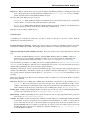
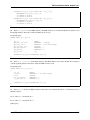
Click on both sections to reveal the results. You should see something similar to the screenshot below.
Fig. 2.17: Analysis Report for Use Case 1
Let’s first look at the results of the non-repeated tests. You can see that there seems to be a strong preference for the
corners of a SETL-plate (see Default plate areas for an overview of the plate areas). I say strong, because the P-value
is very low (P < 0.1%). At the same time, this species seems to reject the middle areas of the plates (areas C and D).
There is no significance for area B, so it makes sense that the combination A+B returns significant preference. This
significance is caused by area A, and not B. The same can be said for B+C+D. The significance is caused by the areas
C+D. Area A+B+C returns non-significant. This is because both A and C have a significance, but in the opposite
directions. B has again no influence because it’s not significant.
Remember that these are the results of the non-repeated tests. The results with very low P-values are pretty solid, even
though the expected values were calculated randomly. But this cannot be said for P-values that are close to the alpha
level (5% by default). In that case the significance result could be a coincidence. This is why the results of repeated
tests are included as well.
The Wilcoxon test was repeated a number of times. And before each repeat, the expected values are re-calculated. By
default, the number of repeats is set to 10.
Let’s have a look at the results of the repeated tests. If you look at the repeat results for plate area A, you’ll see that
out of 10 repeats, 10 were found to be significant (P < 5%). And out of these 10 significant results, all 10 showed a
preference for the area. Based on this result, we can almost safely say that the results we found are not a coincidence.
I say almost, because a total of 10 repeats is very low. To be even more sure, you can set the number of repeats to a
higher value in the Preferences dialog.
Conclusion The species of the genus Obelia have a strong preference for the corners (area A) of SETL-plates, and
a strong rejection for the middle (areas C+D) of SETL-plates. The species don’t seem to have a preference for the
borders (area B).
Use Case 2: Attraction of Species (intra-specific)
Research Question “Does Balanus crenatus from the location Aquadome Grevelingen attract individuals of its own
kind?”
Performing the analysis Analysis “Attraction of Species (intra-specific)” can be used to determine if a species
attracts or repels individuals of its own kind.
For this analysis, we can define the following hypotheses:
28
Chapter 2. Documentations
SETLyze Documentation, Release 1.0.1
Null hypothesis The species in question settles at random areas of SETL-plates, unregarded the presence of other
individuals of its own kind.
Alternative hypothesis The species attracts (observed mean < expected mean) or repels (observed mean > expected
mean) individuals of its own kind.
The analysis uses the P-value to decide which hypothesis is true.
P >= alpha level Assume that the null hypothesis is true.
P < alpha level Assume that the alternative hypothesis is true.
To find an answer to this research question, we’re going to run the analysis on Balanus crenatus from the location
Aquadome Grevelingen.
Start SETLyze, and from the main window select analysis “Attraction within Species”. Then click the OK button
to start the selected analysis. The Locations Selection dialog will now show up. If this is your first time running
SETLyze, then the list of locations will be empty. Clicking the “Load Data” button opens the Load Data dialog. Use
this dialog to load your SETL data. For this example, we’ll use the test data provided with SETLyze.
Note: On Windows, the test data can be found in the sub folder “test-data” of the directory to where you installed
SETLyze (e.g. C:\Program Files\GiMaRIS\SETLyze\test-data\).
On Linux, the “test-data” folder can be found in the source package.
Once the SETL data is loaded, you should see a list of all locations. You can now select the locations from which you
want to select species. For this example, we’re just interested in data from the location Aquadome Grevelingen. Select
“Aquadome, Grevelingen” from the list. Press the Continue button.
The Species Selection dialog should now be displayed. By default, the species are sorted by their scientific name.
Select the species “Balanus crenatus”. Press the Continue button to start the calculations for this analysis.
In a few seconds you should be presented with the Analysis Report dialog. This dialog shows the results for the
analysis.
Results For this analysis, two different statistical hypothesis tests are performed; the Wilcoxon rank-sum test and
Pearson’s Chi-squared test. The following sections should be present in the report dialog:
• Wilcoxon rank sum test with continuity correction
• Wilcoxon rank sum test with continuity correction (repeated)
• Chi-squared test for given probabilities
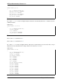
Let’s first have a look at the results of the Wilcoxon tests. Click on both Wilcoxon sections to reveal the results. You
should see something similar to the screenshot below.
Fig. 2.18: Analysis Report for Use Case 2 - Wilcoxon tests
2.2. User Manual
29
SETLyze Documentation, Release 1.0.1
Let’s first look at the results of the non-repeated tests. You’ll see that most results are non-significant. There might
be a few exceptions, but these could have other causes then attraction/repuslion. For example, some parts of the
SETL-plates might be coverd with another species, making it simply impossible for Balanus crenatus to settle there.
So these are the results of the non-repeated tests. The results with very low P-values are pretty solid, even though the
expected values were calculated randomly. But this cannot be said for P-values that are close to the alpha level (5%
by default). In that case the significance result could be a coincidence. This is why the results of repeated tests should
be taken into account as well.
The Wilcoxon test was repeated a number of times. And before each repeat, the expected values are re-calculated. By
default, the number of repeats is set to 10.
Let’s have a look at the results of the repeated tests. Notice that sometimes the test does return significant. If you
however find that the test returns non-significant far more often than significant, you could conclude that there is no
significance, and therefor assume that the null hypothesis is true.
Then there are the results of the Chi-squared tests. While the Wilcoxon test looks at the distribution of spot distances
(the measurements), the Chi-quared test looks at the frequencies at which spot distances occur. The observed frequencies are being compared to the expected frequencies. This again leads to P-values which can be used to determine
which hypothesis is true. Because the expected values are fixed, repeats aren’t necessary for this test.
Fig. 2.19: Analysis Report for Use Case 2 - Chi-squared tests
In this case, the Chi-squared test gives similar results to the Wilcoxon test. It turns out however that this method is less
sensitive to differences in samples.
Conclusion Balanus crenatus doesn’t seem to attract or repel individuals of its own kind.
2.3 SETLyze Developer Guide
Welcome to the Developer Guide for SETLyze. This document describes the SETLyze internals. It’s meant for people
who are involved in the development process of SETLyze. It should be easy for a new developer to pick up where
the last SETLyze developer left off. The purpose of this guide is to give the new developer full understanding of
SETLyze’s internals, its programming style, what’s unfinished, et cetera.
2.3.1 Getting Started
Obtaining the source code
The source code for SETLyze is currently hosted on GitHub. The project page can be found at the following URL:
https://github.com/figure002/setlyze
30
Chapter 2. Documentations
SETLyze Documentation, Release 1.0.1
The source code is version controlled with Git. You’ll need to install Git before you can start working on SETLyze.
Go to http://git-scm.com/ to get started with Git.
If you are new to using Git, there is a well written online book Pro Git which explains everything you need to know
about using Git. At least read through the Getting Started section.
Once you have Git installed and properly setup, you can obtain a copy of the source code for SETLyze with the
following command
git clone git://github.com/figure002/setlyze.git
Navigating the SETLyze folder
The key files in SETLyze’s root folder are:
src/setlyze/ This is SETLyze’s main code base. This package folder contains all of SETLyze’s modules. This is the
folder where you’ll be editing most Python source files for SETLyze.
src/setlyze.pyw This is SETLyze’s executable. This is what you’ll run to start SETLyze.
src/setlyze/docs/html/ This folder contains the documentation for SETLyze. This includes the User Manual and the
Developer Guide. You can view the manual by (double) clicking index.html. This should open the documentation in your web browser.
src/doc-src/ This folder contains the files used to build the documentation. This is done using Sphinx. Some parts of
the documentation are from .rst-files within this folder, others are extracted from the documentation strings
within the program source code.
README.md This text file contains a short description of the program and directs you to other documentation.
COPYING This text file contains the license for SETLyze. SETLyze is released under the GNU General Public
License version 3.
INSTALL Text file with installation instructions for SETLyze.
Technical Design
SETLyze comes with a Technical Design; a visual representation of SETLyze’s design parts (functions/classes/GUI’s) interconnected by arrows representing the application’s functions and work flow. All design
parts are numbered. The same numbers can be found in the SETLyze’s source code. This means that the different
design parts of the Technical Design can be easily linked to the corresponding source code.
The Technical Design provides an easy to understand overview of the application for users, but is also of great value
to developers. It makes it easier to get a basic understanding of how the application works by looking at the Technical Design. If the developer is interested in a specific part of the application, he or she can easily navigate to the
corresponding description and source code by the reference numbers used in the Technical Design.
Both the descriptions and source codes for the design parts in the Technical Design are browsable using this documentation. Read the “Design Parts” section below.
Design Parts
The links below will guide you to the different design parts present in the Technical Design. You just have to click in
the the number for that design part. Clicking on a design part will show you its description. Next to the description is
a link “[source]” which links to the corresponding source code.
Design Parts
2.3. SETLyze Developer Guide
31
SETLyze Documentation, Release 1.0.1
Design Part #
1.0
1.1
1.2
1.3
1.3.1
1.3.2
1.3.3
1.4
1.4.1
1.4.2
1.4.3
1.5
1.5.1
1.5.2
1.5.3
1.11
1.12
1.13
1.14
1.15
1.17
1.19.1
1.20
1.22
1.23
1.24
1.27
1.28
1.29
1.31
1.32
1.33
1.34.1
1.34.2
1.35.1
1.35.2
1.36.1
1.36.2
1.37.1
1.37.2
1.38
1.39
1.41.1
1.42
1.43
1.44
1.45
1.48
1.50
1.51
32
Reference
The executable for SETLyze (setlyze.pyw).
The main() function in the executable.
setlyze.database.MakeLocalDB
setlyze.analysis.spot_preference
setlyze.analysis.spot_preference.Begin
setlyze.analysis.spot_preference.BeginBatch
setlyze.analysis.spot_preference.Analysis
setlyze.analysis.attraction_intra
setlyze.analysis.attraction_intra.Begin
setlyze.analysis.attraction_intra.BeginBatch
setlyze.analysis.attraction_intra.Analysis
setlyze.analysis.attraction_inter
setlyze.analysis.attraction_inter.Begin
setlyze.analysis.attraction_inter.BeginBatch
setlyze.analysis.attraction_inter.Analysis
setlyze.gui.SelectionWindow.on_load_data()
setlyze.report.Report
setlyze.analysis.spot_preference.Analysis.generate_report()
setlyze.analysis.attraction_intra.Analysis.generate_report()
setlyze.analysis.attraction_inter.Analysis.generate_report()
setlyze.report.export()
setlyze.database.AccessLocalDB.set_species_spots()
setlyze.database.AccessDBGeneric.make_plates_unique()
setlyze.analysis.attraction_intra.Analysis.calculate_distances_intra()
setlyze.analysis.attraction_intra.Analysis.calculate_distances_intra_expected
setlyze.analysis.attraction_intra.Analysis.calculate_significance()
setlyze.analysis.attraction_inter.Analysis.calculate_distances_inter()
setlyze.database.AccessLocalDB
setlyze.database.AccessRemoteDB
setlyze.database.MakeLocalDB.run()
setlyze.database.MakeLocalDB.insert_from_data_files()
setlyze.database.MakeLocalDB.insert_from_db()
setlyze.database.MakeLocalDB.insert_locations_from_csv()
setlyze.database.MakeLocalDB.insert_locations_from_xls()
setlyze.database.MakeLocalDB.insert_species_from_csv()
setlyze.database.MakeLocalDB.insert_species_from_xls()
setlyze.database.MakeLocalDB.insert_plates_from_csv()
setlyze.database.MakeLocalDB.insert_plates_from_xls()
setlyze.database.MakeLocalDB.insert_records_from_csv()
setlyze.database.MakeLocalDB.insert_records_from_xls()
setlyze.database.MakeLocalDB.create_new_db()
setlyze.gui.SelectionWindow.update_tree()
setlyze.database.AccessLocalDB.get_record_ids()
setlyze.gui.SelectLocations.create_model()
setlyze.gui.SelectSpecies.create_model()
setlyze.gui.SelectionWindow.on_continue()
setlyze.gui.SelectionWindow.on_back()
setlyze.report.Report
setlyze.report.Report.set_location_selections()
setlyze.report.Report.set_species_selections()
Continued on next pa
Chapter 2. Documentations
SETLyze Documentation, Release 1.0.1
Design Part #
1.52
1.53
1.54
1.55
1.56
1.57
1.58
1.59
1.60
1.62
1.63
1.64
1.65
1.68
1.69
1.70
1.72
1.73
1.74
1.75
1.76
1.77
1.78
1.79
1.80
1.81
1.83
1.84
1.85
1.86
1.87
1.88
1.89
1.90
1.91
1.92
1.93
1.94
1.95
1.96
1.98
1.99
1.100
1.101
1.102
1.103
1.104
1.105
Table 2.1 – continued from previous page
Reference
setlyze.report.Report.set_spot_distances_observed()
setlyze.report.Report.set_spot_distances_expected()
setlyze.report.Report.set_plate_areas_definition()
setlyze.report.Report.set_area_totals_observed()
setlyze.report.Report.set_area_totals_expected()
setlyze.config.ConfigManager
setlyze.analysis.spot_preference.Analysis.run()
setlyze.analysis.attraction_intra.Analysis.run()
setlyze.analysis.attraction_inter.Analysis.run()
setlyze.analysis.spot_preference.Analysis.set_plate_area_totals_observed()
setlyze.analysis.spot_preference.Analysis.set_plate_area_totals_expected()
setlyze.analysis.spot_preference.Analysis.get_defined_areas_totals_observed()
setlyze.analysis.spot_preference.Analysis.repeat_wilcoxon_test()
setlyze.analysis.common.PrepareAnalysis.on_display_results()
setlyze.analysis.attraction_inter.Analysis.calculate_distances_inter_expected
setlyze.report.Report.set_statistics()
setlyze.report.Report.set_analysis()
setlyze.database.AccessDBGeneric.fill_plate_spot_totals_table()
setlyze.analysis.attraction_inter.Analysis.calculate_significance()
setlyze.database.MakeLocalDB.create_table_info()
setlyze.database.MakeLocalDB.create_table_localities()
setlyze.database.MakeLocalDB.create_table_species()
setlyze.database.MakeLocalDB.create_table_plates()
setlyze.database.MakeLocalDB.create_table_records()
setlyze.database.AccessLocalDB.create_table_species_spots_1()
setlyze.database.AccessLocalDB.create_table_species_spots_2()
setlyze.database.AccessLocalDB.create_table_spot_distances_observed()
setlyze.database.AccessLocalDB.create_table_spot_distances_expected()
setlyze.database.AccessLocalDB.create_table_plate_spot_totals()
setlyze.gui.SelectAnalysis
setlyze.gui.SelectLocations
setlyze.gui.SelectSpecies
setlyze.gui.Report
setlyze.gui.LoadData
setlyze.gui.DefinePlateAreas
setlyze.gui.ProgressDialog
setlyze.database.get_database_accessor()
setlyze.std.Sender
setlyze.database.AccessDBGeneric.get_locations()
setlyze.database.AccessLocalDB.get_species()
setlyze.analysis.spot_preference.Analysis.calculate_significance_wilcoxon()
setlyze.analysis.spot_preference.Analysis.calculate_significance_chisq()
setlyze.analysis.spot_preference.Analysis.wilcoxon_test_for_repeats()
setlyze.analysis.spot_preference.Analysis.get_area_probabilities()
setlyze.analysis.attraction_intra.Analysis.wilcoxon_test_for_repeats()
setlyze.analysis.attraction_intra.Analysis.repeat_wilcoxon_test()
setlyze.analysis.attraction_inter.Analysis.wilcoxon_test_for_repeats()
setlyze.analysis.attraction_inter.Analysis.repeat_wilcoxon_test()
1.x Modules, Classes & Functions
2.3. SETLyze Developer Guide
33
SETLyze Documentation, Release 1.0.1
2.x Data Storage Places
Design Parts: Data The design parts in this overview describes all technical design parts representing data used in
SETLyze. This includes database tables, application variables, and data files.
2.x Data Storage Places
2.0 Table setl_records in the SETL database. The SETL database can be either the MS Access database or the
PostgreSQL database. This table contains the SETL records.
PostgreSQL query:
CREATE TABLE setl_records
(
rec_id
SERIAL,
rec_pla_id
INTEGER NOT NULL,
rec_spe_id
INTEGER NOT NULL,
rec_unknown
BOOLEAN,
rec_o
BOOLEAN,
rec_r
BOOLEAN,
rec_c
BOOLEAN,
rec_a
BOOLEAN,
rec_e
BOOLEAN,
rec_sur_unknown
BOOLEAN,
rec_sur1
BOOLEAN,
rec_sur2
BOOLEAN,
rec_sur3
BOOLEAN,
rec_sur4
BOOLEAN,
rec_sur5
BOOLEAN,
rec_sur6
BOOLEAN,
rec_sur7
BOOLEAN,
rec_sur8
BOOLEAN,
rec_sur9
BOOLEAN,
rec_sur10
BOOLEAN,
rec_sur11
BOOLEAN,
rec_sur12
BOOLEAN,
rec_sur13
BOOLEAN,
rec_sur14
BOOLEAN,
rec_sur15
BOOLEAN,
rec_sur16
BOOLEAN,
rec_sur17
BOOLEAN,
rec_sur18
BOOLEAN,
rec_sur19
BOOLEAN,
rec_sur20
BOOLEAN,
rec_sur21
BOOLEAN,
rec_sur22
BOOLEAN,
rec_sur23
BOOLEAN,
rec_sur24
BOOLEAN,
rec_sur25
BOOLEAN,
rec_1st
BOOLEAN,
rec_2nd
BOOLEAN,
rec_v
BOOLEAN,
rec_photo_nrs
VARCHAR(100),
rec_remarks
VARCHAR(100),
CONSTRAINT rec_id_pk PRIMARY KEY (rec_id),
34
Chapter 2. Documentations
SETLyze Documentation, Release 1.0.1
CONSTRAINT rec_pla_id_fk FOREIGN KEY (rec_pla_id)
REFERENCES setl_plates (pla_id)
ON DELETE NO ACTION
ON UPDATE NO ACTION,
CONSTRAINT rec_spe_id_fk FOREIGN KEY (rec_spe_id)
REFERENCES setl_species (spe_id)
ON DELETE NO ACTION
ON UPDATE NO ACTION
);
2.1 Table setl_species in the SETL database. The SETL database can be either the MS Access database or the
PostgreSQL database. This table contains the SETL species records.
PostgreSQL query:
CREATE TABLE setl_species
(
spe_id
spe_name_venacular
spe_name_latin
spe_invasive_in_nl
spe_description
spe_remarks
spe_picture
SERIAL,
VARCHAR(100) UNIQUE,
VARCHAR(100) NOT NULL UNIQUE,
BOOLEAN,
VARCHAR(300),
VARCHAR(160),
OID,
CONSTRAINT spe_id_pk PRIMARY KEY (spe_id)
);
2.2 Table setl_localities in the SETL database. The SETL database can be either the MS Access database
or the PostgreSQL database. This table contains the SETL locality records.
PostgreSQL query:
CREATE TABLE setl_localities
(
loc_id
SERIAL,
loc_name
VARCHAR(100) NOT NULL UNIQUE,
loc_nr
INTEGER,
loc_coordinates
VARCHAR(100),
loc_description
VARCHAR(300),
CONSTRAINT loc_id_pk PRIMARY KEY (loc_id)
);
2.3 Table species in the local SQLite database. This table is automatically filled from 2.1 when the user starts a
SETLyze analysis.
2.3.1 Same as 2.3, but filled from 2.1.
2.3.2 Same as 2.3, but filled from 2.19.
SQLite query:
2.3. SETLyze Developer Guide
35
SETLyze Documentation, Release 1.0.1
CREATE TABLE species
(
spe_id INTEGER PRIMARY KEY,
spe_name_venacular VARCHAR,
spe_name_latin VARCHAR,
spe_invasive_in_nl INTEGER,
spe_description VARCHAR,
spe_remarks VARCHAR
);
2.4 Table localities in the local SQLite database. This table is automatically filled from 2.2 when the user starts
a SETLyze analysis.
SQLite query:
CREATE TABLE localities
(
loc_id INTEGER PRIMARY KEY,
loc_name VARCHAR,
loc_nr VARCHAR,
loc_coordinates VARCHAR,
loc_description VARCHAR
);
2.4.1 Same as 2.4, but filled from 2.2.
2.4.2 Same as 2.4, but filled from 2.18.
2.5 Table records in the local SQLite database. This table is only filled if the user selected CSV files to import
SETL data from. By default this table is empty, and the records data from 2.0 is used.
SQLite query:
CREATE TABLE records
(
rec_id INTEGER PRIMARY KEY,
rec_pla_id INTEGER,
rec_spe_id INTEGER,
rec_unknown INTEGER,
rec_o INTEGER,
rec_r INTEGER,
rec_c INTEGER,
rec_a INTEGER,
rec_e INTEGER,
rec_sur_unknown INTEGER,
rec_sur1 INTEGER,
rec_sur2 INTEGER,
rec_sur3 INTEGER,
rec_sur4 INTEGER,
rec_sur5 INTEGER,
rec_sur6 INTEGER,
rec_sur7 INTEGER,
rec_sur8 INTEGER,
rec_sur9 INTEGER,
rec_sur10 INTEGER,
36
Chapter 2. Documentations
SETLyze Documentation, Release 1.0.1
rec_sur11 INTEGER,
rec_sur12 INTEGER,
rec_sur13 INTEGER,
rec_sur14 INTEGER,
rec_sur15 INTEGER,
rec_sur16 INTEGER,
rec_sur17 INTEGER,
rec_sur18 INTEGER,
rec_sur19 INTEGER,
rec_sur20 INTEGER,
rec_sur21 INTEGER,
rec_sur22 INTEGER,
rec_sur23 INTEGER,
rec_sur24 INTEGER,
rec_sur25 INTEGER,
rec_1st INTEGER,
rec_2nd INTEGER,
rec_v INTEGER
);
2.6 A list [<selection-1>,<selection-2>] for storing a maximum of two location selections.
<selection-1> and <selection-2> are lists of integers representing location IDs. These IDs are the same
as the IDs in column loc_id in 2.2 and 2.4.
If no location selections are made yet, this variable has the value [None,None].
Get the value with setlyze.config.ConfigManager.get()
setlyze.config.cfg.get('locations-selection', slot=int)
Set the value with setlyze.config.ConfigManager.set()
setlyze.config.cfg.set('locations-selection', list, slot=int)
2.7 A list [<selection-1>,<selection-2>] for storing a maximum of two species selections.
<selection-1> and <selection-2> are lists of integers representing species IDs. These IDs are the same
as the IDs in column spe_id in 2.1 and 2.3.
Get the value with setlyze.config.ConfigManager.get()
setlyze.config.cfg.get('species-selection', slot=int)
Set the value with setlyze.config.ConfigManager.set()
setlyze.config.cfg.set('species-selection', list, slot=int)
2.9 Table species_spots_1 in the local database containing the SETL records for the first selection of species
and locations.
This table does not contain the complete records, but just the plate ID and the 25 record surfaces.
SQLite query:
CREATE TABLE species_spots_1
(
id INTEGER PRIMARY KEY,
rec_pla_id INTEGER,
2.3. SETLyze Developer Guide
37
SETLyze Documentation, Release 1.0.1
rec_sur1 INTEGER,
rec_sur2 INTEGER,
rec_sur3 INTEGER,
rec_sur4 INTEGER,
rec_sur5 INTEGER,
rec_sur6 INTEGER,
rec_sur7 INTEGER,
rec_sur8 INTEGER,
rec_sur9 INTEGER,
rec_sur10 INTEGER,
rec_sur11 INTEGER,
rec_sur12 INTEGER,
rec_sur13 INTEGER,
rec_sur14 INTEGER,
rec_sur15 INTEGER,
rec_sur16 INTEGER,
rec_sur17 INTEGER,
rec_sur18 INTEGER,
rec_sur19 INTEGER,
rec_sur20 INTEGER,
rec_sur21 INTEGER,
rec_sur22 INTEGER,
rec_sur23 INTEGER,
rec_sur24 INTEGER,
rec_sur25 INTEGER
);
2.9.1 Same as 2.9, but with unique plates.
2.9.2 Same as 2.9, but with plates with just one spot removed.
2.10 Table species_spots_2 in the local database containing the SETL records for the second selection of
species and locations.
This table does not contain the complete records, but just the plate ID and the 25 record surfaces.
SQLite query:
CREATE TABLE species_spots_2
(
id INTEGER PRIMARY KEY,
rec_pla_id INTEGER,
rec_sur1 INTEGER,
rec_sur2 INTEGER,
rec_sur3 INTEGER,
rec_sur4 INTEGER,
rec_sur5 INTEGER,
rec_sur6 INTEGER,
rec_sur7 INTEGER,
rec_sur8 INTEGER,
rec_sur9 INTEGER,
rec_sur10 INTEGER,
rec_sur11 INTEGER,
rec_sur12 INTEGER,
rec_sur13 INTEGER,
rec_sur14 INTEGER,
38
Chapter 2. Documentations
SETLyze Documentation, Release 1.0.1
rec_sur15
rec_sur16
rec_sur17
rec_sur18
rec_sur19
rec_sur20
rec_sur21
rec_sur22
rec_sur23
rec_sur24
rec_sur25
INTEGER,
INTEGER,
INTEGER,
INTEGER,
INTEGER,
INTEGER,
INTEGER,
INTEGER,
INTEGER,
INTEGER,
INTEGER
);
2.10.1 Same as 2.10, but with unique plates.
2.10.2 Same as 2.10, but with plates with just one spot removed.
2.12 Table spot_distances_observed in the local database containing the observed spot distances.
Contains the spot distances for the records in 2.9 if created by calculate_distances_intra().
If the table is created by calculate_distances_inter(), the table contains the distances between spots in 2.9
and 2.10.
SQLite query:
CREATE TABLE spot_distances_observed
(
id INTEGER PRIMARY KEY,
rec_pla_id INTEGER,
distance REAL
);
2.13 Table spot_distances_expected in the local database. Has the same design as 2.12, but contains random generated spot distances instead. These random generated spot distances will serve as the expected spot distances.
SQLite query:
CREATE TABLE spot_distances_expected
(
id INTEGER PRIMARY KEY,
rec_pla_id INTEGER,
distance REAL
);
2.14 Table info in the local SQLite database for storing basic information about the local database.
SQLite query:
CREATE TABLE info
(
id INTEGER PRIMARY KEY,
name VARCHAR,
value VARCHAR
);
2.3. SETLyze Developer Guide
39
SETLyze Documentation, Release 1.0.1
This information includes its creation date, the data source, and a version number. The data source is a string which
has the same design as 2.22. You can insert the data source with the following SQLite query
cursor.execute( "INSERT INTO info VALUES (null, 'source', ?)", [setlyze.config.cfg.get('data-source')
Giving a version number to the local database could be useful in the future. We can then notify the user if the
local database is too old, followed by creating a new local database. This would only work if the version for the
database is incremented each time you change the design of the local database. To do this, edit the version number in
create_table_info(). The version number can be inserted with
cursor.execute("INSERT INTO info VALUES (null, 'version', ?)", [db_version])
The creation date and data source is inserted by the methods insert_from_csv() and insert_from_db().
The date can be inserted with
cursor.execute( "INSERT INTO info VALUES (null, 'date', date('now'))" )
2.15 Table setl_plates in the SETL database. The SETL database can be either the MS Access database or the
PostgreSQL database. This table contains the SETL plate records.
PostgreSQL query:
CREATE TABLE setl_plates
(
pla_id
pla_loc_id
pla_setl_coordinator
pla_nr
pla_deployment_date
pla_retrieval_date
pla_water_temperature
pla_salinity
pla_visibility
pla_remarks
SERIAL,
INTEGER NOT NULL,
VARCHAR(100),
VARCHAR(100),
TIMESTAMP,
TIMESTAMP,
VARCHAR(100),
VARCHAR(100),
VARCHAR(100),
VARCHAR(300),
CONSTRAINT pla_id_pk PRIMARY KEY (pla_id),
CONSTRAINT pla_loc_id_fk FOREIGN KEY (pla_loc_id)
REFERENCES setl_localities (loc_id)
ON DELETE NO ACTION
ON UPDATE NO ACTION
);
2.16 Table plates in the local SQLite database. This table is only filled if the user selected CSV files to import
SETL data from. By default this table is empty, and the plates data from 2.15 is used.
SQLite query:
CREATE TABLE plates
(
pla_id INTEGER PRIMARY KEY,
pla_loc_id INTEGER,
pla_setl_coordinator VARCHAR,
pla_nr VARCHAR,
pla_deployment_date TEXT,
pla_retrieval_date TEXT,
pla_water_temperature VARCHAR,
pla_salinity VARCHAR,
pla_visibility VARCHAR,
40
Chapter 2. Documentations
SETLyze Documentation, Release 1.0.1
pla_remarks VARCHAR
);
2.17 Links to an instance of xml.dom.minidom.Document.
It’s a XML DOM (Document Object Model) object containing the analysis settings and results. This XML DOM object is generated by
setlyze.report.ReportGenerator.
Get the value with setlyze.config.ConfigManager.get()
setlyze.config.cfg.get('analysis-report')
Set the value with setlyze.config.ConfigManager.set()
setlyze.config.cfg.set('analysis-report', value)
2.18 CSV file containing the locality records exported from the MS Access SETL database.
If exported from the MS Access SETL database, the CSV file must have the format
LOC_id;LOC_name;LOC_nr;LOC_coordinates;LOC_description
2.19 CSV file containing the species records exported from the MS Access SETL database.
If exported from the MS Access SETL database, the CSV file must have the format
SPE_id;SPE_name_venacular;SPE_name_latin;SPE_invasive_in_NL;SPE_description;SPE_remarks;SPE_picture
2.20 CSV file containing the plate records exported from the MS Access SETL database.
If exported from the MS Access SETL database, the CSV file must have the format
PLA_id;PLA_LOC_id;PLA_SETL_coordinator;PLA_nr;PLA_deployment_date;PLA_retrieval_date;PLA_water_temper
2.21 CSV file containing the SETL records exported from the MS Access SETL database.
If exported from the MS Access SETL database, the CSV file must have the format
REC_id;REC_PLA_id;REC_SPE_id;REC_?;REC_O;REC_R;REC_C;REC_A;REC_E;REC_sur?;REC_sur1;REC_sur2;REC_sur3;
2.22 A string variable representing the current data source.
Can be either setl-database or data-files. Several application functions check this variable to figure out
where to obtain data from. The first means the PostgreSQL SETL database, and the second from user selected CSV
files exported from the MS Access SETL database.
This variable should be set whenever the data source has changed.
Get the value with setlyze.config.ConfigManager.get()
setlyze.config.cfg.get('data-source')
Set the value with setlyze.config.ConfigManager.set()
setlyze.config.cfg.set('data-source', value)
2.3. SETLyze Developer Guide
41
SETLyze Documentation, Release 1.0.1
2.23 Table spot_distances in the local database containing all possible pre-calculated spot distances.
SQLite query:
CREATE TABLE spot_distances
(
id INTEGER PRIMARY KEY,
delta_x INTEGER,
delta_y INTEGER,
distance REAL
);
Each distance in this table is coupled to a horizontal and a vertical spot difference. The distances are pre-calculated by
setlyze.std.distance(). In other words, if we have two spots, and we know the horizontal difference (∆x)
and the vertical difference (∆y), we can look up the corresponding distance in the spot_distances table.
Deprecated since version 0.1: A performance test showed that retrieving pre-calculated spot distances from the
database is much slower than calculating them on run time.
2.24 Variable of type dict containing the plate areas definition for analysis 1.
The dictionary has the format
{
'area1':
'area2':
'area3':
'area4':
}
list,
list,
list,
list
Where list is a list of strings. The possible strings are A, B, C and D. Each letter represents a surface on a SETL
plate. For a clearer picture, refer to Default plate areas.
The default value for the plate areas definition is
{
'area1':
'area2':
'area3':
'area4':
}
['A'],
['B'],
['C'],
['D']
Using setlyze.gui.DefinePlateAreas, the user can change this definition. The user could for example
combine the surfaces A and B, meaning the value for this variable becomes
{
'area1': ['A', 'B'],
'area3': ['C'],
'area4': ['D']
}
Keep in mind that the dictionary keys (area1, area2, ..) don’t have any meaning. They just make it possible to destinct
between the plate areas.
Get the value with setlyze.config.ConfigManager.get()
setlyze.config.cfg.get('plate-areas-definition')
Set the value with setlyze.config.ConfigManager.set()
42
Chapter 2. Documentations
SETLyze Documentation, Release 1.0.1
setlyze.config.cfg.set('plate-areas-definition', value)
2.25 An application variable that contains the observed species totals for each user defined plate area. Keep in mind
that this is not the number of individual organisms found on the plate areas, as the records just tell the presence of a
species. So it tells how many times the presence of a species was found on each user defined plate area.
This is what the value can look like
{
'area4':
'area1':
'area2':
'area3':
}
52,
276,
751,
457
Namespace: setlyze.analysis.spot_preference.Start.areas_totals_observed
2.26 An application variable that contains the expected species totals for each plate area. Keep in mind that this not
the number of individuals found on the plate area, as the records just tell the presence of a species.
This is what the value can look like
{
'area4':
'area1':
'area2':
'area3':
}
61.439999999999998,
245.75999999999999,
737.27999999999997,
491.51999999999998
Namespace: setlyze.analysis.spot_preference.areas_totals_expected
2.27 The element location_selections in the XML DOM report that contains the user selected locations.
2.28 The element species_selections in the XML DOM report that contains the user selected species.
2.29 The element spot_distances_observed in the XML DOM report that contains the actual spot distances.
2.30 The element spot_distances_expected in the XML DOM report that contains the expected spot distances.
2.31 The element plate_areas_definition in the XML DOM report that contains the user defined plate
areas definition.
2.32 The element area_totals_observed in the XML DOM report that contains the actual species totals per
plate area.
2.33 The element area_totals_expected in the XML DOM report that contains the expected species totals
per plate area.
2.3. SETLyze Developer Guide
43
SETLyze Documentation, Release 1.0.1
2.34 The element statistics_normality in the XML DOM report that contains the statistic results for the
normality tests.
2.35 The element statistics_significance in the XML DOM report that contains the statistic results for
the significance tests.
2.36 Analysis variable that contains the statistic results for the normality tests.
Namespace: setlyze.analysis.attraction_intra.Begin.statistics[’normality’]
2.37 Analysis variable that contains the statistic results for the significance tests.
Namespace: setlyze.analysis.attraction_intra.Begin.statistics[’significance’]
2.38 The element analysis in the XML DOM report that contains the name of the analysis.
2.39 Table plate_spot_totals in the local database for the number of positive spots for each plate ID in the
tables 2.9 and/or 2.10.
Column n_spots_a is for the spots in 2.9, and column n_spots_b for the spots in 2.10.
SQLite query:
CREATE TABLE plate_spot_totals
(
pla_id INTEGER PRIMARY KEY,
n_spots_a INTEGER,
n_spots_b INTEGER
);
2.40 A XML file containing all data elements from 2.17.
2.41 Table plate_area_totals_observed in the local SQLite database. This table contains the number of
positive spots for each default plate area (A, B, C, and D) for each plate that matches the species selection.
This table is filled by set_plate_area_totals_observed().
SQLite query:
CREATE TABLE plate_area_totals_observed (
pla_id INTEGER PRIMARY KEY,
area_a INTEGER,
area_b INTEGER,
area_c INTEGER,
area_d INTEGER
);
2.42 Table plate_area_totals_expected in the local SQLite database.
This table contains the number of expected positive spots for each default plate area (A, B, C, and D) per plate that
matches the species selection. The expected spots are calculated with a random generator. The random generator
randomly puts an equal number of positive spots on a virtual plate, then calcualtes the number of positive spots for
each plate area. This is done for all plates mathching a species selection.
44
Chapter 2. Documentations
SETLyze Documentation, Release 1.0.1
This table is filled by set_plate_area_totals_expected().
SQLite query:
CREATE TABLE plate_area_totals_expected (
pla_id INTEGER PRIMARY KEY,
area_a INTEGER,
area_b INTEGER,
area_c INTEGER,
area_d INTEGER
);
3.x Graphical User Interfaces
Design Part #
3.0
3.1
3.2
3.3
3.4
3.5
3.6
3.7
Reference
Analysis Selection dialog
Locations Selection dialog
Species Selection dialog
Analysis Report dialog
Load Data dialog
Define Plate Areas dialog
Preferences dialog
Batch Mode dialog
4.x Documents
Design Parts: Documents The design parts in this overview describes all technical design parts representing documents created by SETLyze.
4.x Documents
4.0 The analysis report. The report can be exported in reStructuredText format.
Navigating the SETLyze Code Base
SETLyze’s many functions and classes are stored in different modules. Classes and functions with similar functions
are placed in the same module.
Below is an overview of all modules for SETLyze. You can click on a module to get a description of that module and
all its elements. You can even view the source-code for a specific function or class by clicking the [source] link on the
right side of the description.
SETLyze modules
SETLyze Standard Modules This reference manual describes the modules that are part of SETLyze.
setlyze.config — Configuration manager
Author Serrano Pereira, Adam van Adrichem, Fedde Schaeffer
Release 1.0.1
Date July 17, 2015
2.3. SETLyze Developer Guide
45
SETLyze Documentation, Release 1.0.1
Module Contents
setlyze.database — Database access
Author Serrano Pereira, Adam van Adrichem, Fedde Schaeffer
Release 1.0.1
Date July 17, 2015
Module Contents
setlyze.gui — Graphical interfaces
Author Serrano Pereira, Adam van Adrichem, Fedde Schaeffer
Release 1.0.1
Date July 17, 2015
Module Contents
setlyze.locale — English text retrieval
Author Serrano Pereira, Adam van Adrichem, Fedde Schaeffer
Release 1.0.1
Date July 17, 2015
Module Contents This module is for storing and retrieving messages used in SETLyze. The purpose is to have a
standard place for storing these messages. This was basically meant for convenience so the developer doesn’t have to
browse through SETLyze’s code base just to change a sentence.
This module wasn’t created for adding multi-language support, though it can be easily expanded to do so.
setlyze.locale.text(key, *args)
Return the text string from the ENGLISH dictionary where key is key.
A simple example:
>>> import setlyze.locale
>>> setlyze.locale.text('analysis-spot-preference-descr')
'Determine if a species has preference for a specific area on SETL plates.'
Substitution is also supported:
>>> import setlyze.locale
>>> setlyze.locale.text('dummy', "windy with a slight chance of rain")
"And tomorrow's forecast is, windy with a slight chance of rain"
setlyze.report — Generate analysis reports
Author Serrano Pereira
Release 1.0.1
Date July 17, 2015
46
Chapter 2. Documentations
SETLyze Documentation, Release 1.0.1
Module Contents
setlyze.std — Standard functions and classes
Author Serrano Pereira, Adam van Adrichem, Fedde Schaeffer
Release 1.0.1
Date July 17, 2015
Module Contents
Analysis Modules The modules described in this chapter all perform one of SETLyze’s analysis.
setlyze.analysis.attraction_inter — Analysis Attraction between Species
Author Serrano Pereira, Adam van Adrichem, Fedde Schaeffer
Release 1.0.1
Date July 17, 2015
Module Contents
setlyze.analysis.attraction_intra — Analysis Attraction within Species
Author Serrano Pereira, Adam van Adrichem, Fedde Schaeffer
Release 1.0.1
Date July 17, 2015
Module Contents
setlyze.analysis.batch — Batch mode
Author Serrano Pereira
Release 1.0.1
Date July 17, 2015
Module Contents
setlyze.analysis.common — Shared routines for analysis modules
Author Serrano Pereira
Release 1.0.1
Date July 17, 2015
Module Contents
2.3. SETLyze Developer Guide
47
SETLyze Documentation, Release 1.0.1
setlyze.analysis.relations — Analysis Relations between Species
Author Serrano Pereira, Adam van Adrichem, Fedde Schaeffer
Release 1.0.1
Date July 17, 2015
Module Contents
setlyze.analysis.spot_preference — Analysis Spot Preference
Author Serrano Pereira, Jonathan den Boer, Adam van Adrichem, Fedde Schaeffer
Release 1.0.1
Date July 17, 2015
Module Contents
2.3.2 Coding Style Guidelines
Code layout
Please write PEP-8 compliant code.
One often-missed requirement is that the first line of docstrings should be a self-contained one-sentence summary.
We use 4 space indents for blocks, and never use tab characters.
Trailing white space should be avoided, but is allowed. If possible, configure your text editor to automatically remove
trailing spaces and tabs upon saving.
Unix style newlines (LF) are used.
Each file must have a newline at the end of it.
Lines should be no more than 79 characters if at all possible. Use a text editor that has some kind of long line marker
indicating the 79 characters boundary. Lines that continue a long statement may be indented in either of two ways:
within the parenthesis or other character that opens the block, e.g.:
my_long_method(arg1,
arg2,
arg3)
or indented by four spaces:
my_long_method(arg1,
arg2,
arg3)
The first is considered clearer by some people; however it can be a bit harder to maintain (e.g. when the method name
changes), and it does not work well if the relevant parenthesis is already far to the right. Avoid this:
self.legbone.kneebone.shinbone.toebone.shake_it(one,
two,
three)
but rather
48
Chapter 2. Documentations
SETLyze Documentation, Release 1.0.1
self.legbone.kneebone.shinbone.toebone.shake_it(one,
two,
three)
or
self.legbone.kneebone.shinbone.toebone.shake_it(
one, two, three)
For long lists, we like to add a trailing comma and put the closing character on the following line. This makes it easier
to add new items in the future:
from setlyze.std import (
uniqify,
median,
distance,
)
There should be spaces between function parameters, but not between the keyword name and the value:
call(1, 3, cheese=quark)
Module Imports
• Imports should be done at the top-level of the file, unless there is a strong reason to have them lazily loaded
when a particular function runs. Import statements have a cost, so try to make sure they don’t run inside hot
functions.
Naming
Functions, methods or members that are relatively private are given a leading underscore prefix.
We prefer class names to be concatenated capital words (TestCase) and variables, methods and functions to be
lowercase words joined by underscores (revision_id, get_revision).
For the purposes of naming some names are treated as single compound words: “filename”, “revno”.
Consider naming classes as nouns and functions/methods as verbs.
Try to avoid using abbreviations in names, because there can be inconsistency if other people use the full name.
Standard Names
revision_id not rev_id or revid
Functions that transform one thing to another should be named x_to_y (not x2y as occurs in some old code.)
Event and Signal Handling
A large part of SETLyze is controlled with signals and signal handlers.
To emit custom application signals we use setlyze.std.sender.emit().
And to connect a signal to a signal handler, we use setlyze.std.sender.connect().
When signal handlers are no longer
needed, use setlyze.std.sender.disconnect() to disconnect the handler from the signal. Calling setlyze.std.sender.disconnect() should generally be done when the instance that called
setlyze.std.sender.connect() is destroyed.
2.3. SETLyze Developer Guide
49
SETLyze Documentation, Release 1.0.1
License Statement
SETLyze is released under the GNU General Public License version 3. Each file that’s part of SETLyze must have the
copyright notice and copying permission statement included at the top of the file after the encoding declaration. So
the top of each file should look like this:
#!/usr/bin/env python
# -*- coding: utf-8 -*#
# Copyright 2010, GiMaRIS <[email protected]>
#
# This file is part of SETLyze - A tool for analyzing the settlement
# of species on SETL plates.
#
# SETLyze is free software: you can redistribute it and/or modify
# it under the terms of the GNU General Public License as published by
# the Free Software Foundation, either version 3 of the License, or
# (at your option) any later version.
#
# SETLyze is distributed in the hope that it will be useful,
# but WITHOUT ANY WARRANTY; without even the implied warranty of
# MERCHANTABILITY or FITNESS FOR A PARTICULAR PURPOSE. See the
# GNU General Public License for more details.
#
# You should have received a copy of the GNU General Public License
# along with this program. If not, see <http://www.gnu.org/licenses/>.
2.3.3 Testing and Optimization
The following document describes the steps taken to test and optimize SETLyze.
Testing and Optimization
This document describes the steps taken to test and optimize SETLyze.
Testing
Calculation of expected spot distances Analyses 2 and 3 have a built-in consistency check. In all cases must the
number of calculated expected spot distances be equal to the number of observed spot distances. If this is not the case,
than this indicates a bug in the application. This is what the check looks like:
# Perform a consistency check. The number of observed and
# expected spot distances must always be the same.
count_observed = len(observed)
count_expected = len(expected)
if count_observed != count_expected:
raise ValueError("Number of observed and expected spot "
"distances are not equal. This indicates a bug "
"in the application.")
Testing spot distances for normal distribution This part describes the method used to test if the spot distances on
a SETL-plate follow a standard normal distribution. The choice of the statistical tests used for some analyis is based
50
Chapter 2. Documentations
SETLyze Documentation, Release 1.0.1
on the results of this test. This is because some statistical tests assume that the samples follow a normal distribution
while some do not.
First step was to calculate the probabilities for the spot distances on a SETL-plate. A Python script was written to
calculate the probabilities for all possible spot distances on a single SETL-plate. This was done for both intra-specific
and inter-specific spot distances. The results were then loaded into R and visualised in a histogram (see Distribution
for intra-specific spot distances and Distribution for inter-specific spot distances).
Fig. 2.20: Distribution for intra-specific spot distances
The frequencies were obtained by calculating all possible distances between two spots if all 25 spots are covered. The
same test was done with different numbers of positive spots randomly placed on a plate with 100.000 repeats. All
resulting distributions are very similar to this figure.
2.3. SETLyze Developer Guide
51
SETLyze Documentation, Release 1.0.1
Fig. 2.21: Distribution for inter-specific spot distances
52
Chapter 2. Documentations
SETLyze Documentation, Release 1.0.1
The frequencies were obtained by calculating all possible distances between two spots with ratio 25:25 (species A and
B have all 25 spots covered). The same test was done with different positive spots ratios (spots randomly placed on a
plate, 100.000 repeats). All resulting distributions are very similar to this figure.
The histograms show that there is a tendency towards a normal distrubution, but this is obstructed because of the
limited number of possible spot distances. To test if the distribution of spot distances really don’t follow a standard
normal distribution, we performed the One-sample Kolmogorov-Smirnov test on both (intra and inter) spot distance
samples. This was again done with the use of R. The results are as follows:
> ks.test(dist_intra[,1], 'pnorm', mean=mean(dist_intra[,1]), sd=sd(dist_intra[,1]))
One-sample Kolmogorov-Smirnov test
data: dist_intra[, 1]
D = 0.1419, p-value = 1.133e-05
alternative hypothesis: two-sided
Warning message:
In ks.test(dist_intra[, 1], "pnorm", mean = mean(dist_intra[, 1]),
cannot compute correct p-values with ties
:
> ks.test(dist_inter[,1], 'pnorm', mean=mean(dist_inter[,1]), sd=sd(dist_inter[,1]))
One-sample Kolmogorov-Smirnov test
data: dist_inter[, 1]
D = 0.1188, p-value = 4.403e-08
alternative hypothesis: two-sided
Warning message:
In ks.test(dist_inter[, 1], "pnorm", mean = mean(dist_inter[, 1]),
cannot compute correct p-values with ties
:
So the p-values can’t be correctly computed which might render the results unreliable. So the Shapiro-Wilk normality
test was performed as well:
> shapiro.test(dist_intra[, 1])
Shapiro-Wilk normality test
data: dist_intra[, 1]
W = 0.9512, p-value = 1.955e-08
> shapiro.test(dist_inter[, 1])
Shapiro-Wilk normality test
data: dist_inter[, 1]
W = 0.9725, p-value = 1.957e-09
Again very low p-values are found, which is why we assume that spot distances on a SETL-plate don’t follow a
standard normal distribution. Hence we chose the Wilcoxon rank-sum test because this test doesn’t assume that data
come from a normal distribution (Dalgaard). Welch’s t-test is an adaptation of Student’s t-test (Wikipedia). And
because Student’s t-test does assume that data come from a normal distribution (Dalgaard), we chose not to use this
test.
Optimization
2.3. SETLyze Developer Guide
53
SETLyze Documentation, Release 1.0.1
Spot distance calculation It was thought that retrieving pre-calculating spot distances from a table in the local
database would be faster than calculating each spot distance on run time. Python’s timeit module was used to find
out which method is faster. For this purpose a small script was written:
#!/usr/bin/env python
import os
import timeit
from sqlite3 import dbapi2 as sqlite
import setlyze.std
connection = sqlite.connect(os.path.expanduser('~/.setlyze/setl_local.db'))
cursor = connection.cursor()
test_record = [1,1,1,1,1,1,1,1,1,1,1,1,1,1,1,1,1,1,1,1,1,1,1,1,1]
def test1():
"""Get pre-calculated spot distances from the local database."""
combos = setlyze.std.get_spot_combinations_from_record(test_record)
for spot1,spot2 in combos:
h,v = setlyze.std.get_spot_position_difference(spot1,spot2)
cursor.execute( "SELECT distance "
"FROM spot_distances "
"WHERE delta_x = ? "
"AND delta_y = ?",
(h,v))
distance = cursor.fetchone()
def test2():
"""Calculate spot distances on run time."""
combos = setlyze.std.get_spot_combinations_from_record(test_record)
for spot1,spot2 in combos:
h,v = setlyze.std.get_spot_position_difference(spot1,spot2)
distance = setlyze.std.distance(h,v)
# Time both tests.
runs = 1000
t = timeit.Timer("test1()", "from __main__ import test1")
print "test1: %f seconds" % (t.timeit(runs)/runs)
t = timeit.Timer("test2()", "from __main__ import test2")
print "test2: %f seconds" % (t.timeit(runs)/runs)
cursor.close()
connection.close()
The first test in the script gets pre-calculated spot distances from the database and the second test calculates spot
distances on run time. The output was as follows:
test1: 0.011350 seconds
test2: 0.003097 seconds
This shows that calculating spot distances on run time is almost 4 times faster than retrieving pre-calculated spot
distances from the database. So the use of the “spot_distances” table was dropped and spot distances are now calculated
on run time.
54
Chapter 2. Documentations
SETLyze Documentation, Release 1.0.1
2.3.4 Distribution
The following document describes how to create the distribution packages and installers for SETLyze.
Distribution of SETLyze
This guide shows the developer how to distribute SETLyze, making it available for the user.
The purpose of this document is to give the developers instructions on how to distribute SETLyze. This includes
building an installer for Windows, and source packages mainly for GNU/Linux users and developers. New developers
will have to do this at some point, so this document was created for their convenience.
Building a Windows Installer
SETLyze should be as easy as possible to install on Windows machines and most users don’t want to worry about
downloading and installing SETLyze’s pre-requisites. Thus a Windows installer (also called a “setup”) which installs
SETLyze along with all its pre-requisites is required. This section explains how to create the Windows installer
for SETLyze using Nullsoft Scriptable Install System (NSIS), a professional open source system to create Windows
installers.
To start off, you’ll need a Windows machine (preferably Windows XP or higher) to build the installer. Once you have
that, read on to the next part.
Preparing your Windows environment Before you can start building the installer, we need to make some preparations. You first need to make sure that SETLyze runs flawlesly on your Windows machine. Let’s try to get SETLyze
running using only the source code. Do not use the Windows installer to get SETLyze running on your system.
First you need to download and install all of SETLyze’s pre-requisites on the Windows machine. You’ll need to
download and install the tools in the order of this list below. Actually the order doesn’t matter much, but the Python
modules (marked with an asterisk) need to be installed after Python itself is installed. It is important that you get the
right versions as well. If no version number is given in the list below, than it means you can get the latest version.
The tools marked with an asterisk (*) are Python modules, meaning they are available for different versions of Python.
Since we’re using Python 2.7, it is required that you download the versions for Python 2.7. Look at the suffix of the
installer’s filenames, they should end with “-py2.7.exe”. Download only 32bit versions of the tools below. The 32bit
installers often have “win32” or “x86” (not “x86-64”) in the filename.
1. Python (>=2.7 & <3)
2. R (=2.12.1)
3. PyGTK (bundle with PyCairo, PyGObject, GTK+ 2.24.0) (=2.24.0) *
4. RPy (>=1.0.3) *
5. xlrd (>=0.8.0) *
6. Python Win32 Extensions (>=218) *
SETLyze will probably run fine with Python 2.6 too, but the latest Python 2.7 is recommended and used in this tutorial.
We are specifically using GTK+ version 2.24.0 for Windows. At the time of writing this there are also GTK+ 2.24.8
and 2.24.10 available for Windows, but we are not using those versions because of a huge memory leak (bug 685959)
that was introduced in GTK+ 2.24.8 (fixed in 2.24.14). The memory leak causes SETLyze to use a huge amount of
memory which results in a crash when running long batch analyses.
Also notice that we are specifically using R version 2.12.1. This is because the RPy module must correspond to the
version of R and Python you have installed. The latest version of RPy at the time of writing this is version 1.0.3, which
has the filename rpy-1.0.3.win32-py2.7-R.2.12.1.exe. This means it requires R version 2.12.1. There
2.3. SETLyze Developer Guide
55
SETLyze Documentation, Release 1.0.1
Fig. 2.22: Screenshot of the Windows installer for SETLyze
56
Chapter 2. Documentations
SETLyze Documentation, Release 1.0.1
is also RPy2, a redesign and rewrite of RPy. During the development of the initial version of SETLyze, it was too hard
to get RPy2 working well on Windows, which is why was decided to use the older but stable RPy. It is possible to
migrate to RPy2 and newer versions of R, but this requires changes in the source code of SETLyze, as RPy2 works
slightly different.
Running and Testing SETLyze Now that you have installed all of SETLyze’s pre-requisites, you can try to run
SETLyze. First obtain a copy of SETLyze’s Git repository (see Obtaining the source code). We will use the SETLyze
Git repository to build the Windows installer.
Note: It is important that you get the Git repository, not just the code from a source package.
The Git repository contains a file src/setlyze.pyw. This is the executable for SETLyze. On Windows, you should
run it with the command python -d src/setlyze.pyw from a DOS window so you can see any error/debug
messages returned by SETLyze. After you have thoroughly tested SETLyze and found no problems or error messages,
you can continue with the next step.
Preparing the Distribution Folder Not all files required for creating a Windows installer are included in the Git
repository for SETLyze. So you need to manually copy some extra files to the folder. First I will explain some of the
important files and folders.
win32/ This folder contains some files required for creating the Windows installer.
win32/dependencies/ This folder is for third party Windows installers of some of SETLyze’s pre-requisites that will
be incorporated in SETLyze’s Windows installer. For SETLyze 1.0, this folder must just contain the installer for
R 2.12.1.
win32/setlyze_setup_modern.nsi This is the NSIS script we will use to build SETLyze’s Windows installer. This
script is a regular text file. You can open it in a text editor (e.g. Notepad++ or gedit). This script contains all the
information required for building the Windows installer.
src/ This folder contains SETLyze’s main code base.
src/build-win32-exe.py This script is used to build the Windows executable for SETLyze. This script uses py2exe
for that. This script is not intended for installing SETLyze.
FYI: It would make more sense to put this file in the ‘win32’ folder, but SETLyze’s module folder
(src/setlyze/) needs to be in the same folder as this script.
src/doc-src/source/ This folder contains the source files of the documentation. The source files end with the extension
”.rst”. You can edit these with a text editor. After editing the source files (*.rst) for the documentation, you
can use the make files (“Makefile” on Linux, “make.bat” on Windows) to generate the actual HTML documentation. Refer to the Sphinx documentation for instructions.
The Makefile contains a custom target html2 which is similar to the default html target, but uses the -E
switch of sphinx-build so that all source files are read. This is useful when some parts of the documentation
aren’t fully updated.
The generated documentation is put in src/setlyze/docs/.
To prepare the folder containing SETLyze’s Git repository for creating distributions, you need to copy the Windows
installer for R 2.12.1 in the win32/dependencies folder. The installer is called R-2.12.1-win.exe and can
be downloaded from the R website.
Building the Windows Executable for SETLyze The next step is to create a Windows executable for SETLyze.
From now on, you need to be at a Windows machine (notice the use of backslashes). At this point, one can start
SETLyze by running setlyze.pyw from the Git repository. So setlyze.pyw is SETLyze’s executable, but it is
a regular Python script, and one needs to have Python and all of SETLyze’s pre-requisites installed to run the script.
2.3. SETLyze Developer Guide
57
SETLyze Documentation, Release 1.0.1
We don’t want Windows users to have to download and install all these extra tools. So before creating the installer,
we’re going to create a special Windows executable (setlyze.exe) which does not require users to have Python
and all the pre-requisites installed (with one exception). For this purpose we’re going to use py2exe. Download the
latest py2exe for Python 2.7 from here and install it on your Windows machine.
Once you have py2exe installed, building the Windows executable should be a breeze with the provided
src\build-win32-exe.py. Open up a DOS window and run the following command:
cd src\
python build-win32-exe.py py2exe
Note: Running Python from the command-line (or DOS) requires that you have Python in your PATH environment
variable. Python is not added to PATH by default. If the above command gives you a message like:
“‘python’ is not recognized as an internal or external command, operable program or batch file.”
then you need to make sure that your computer knows where to find the Python interpreter. To do this you will have
to modify a variable called PATH, which is a list of directories where Windows will look for programs.
The Python on Windows FAQ explains how to do this. Search for “PATH environment variable” on that page (Ctrl+F,
type “PATH environment variable”, hit Enter).
This should create a new folder called src\dist\. Open this folder in Windows Explorer. You should now see a
whole bunch of files, including setlyze.exe.
Go ahead and see if setlyze.exe runs. Double clicking setlyze.exe should open up SETLyze’s main window. You might notice something different though. The dialogs look really ugly. Remember that this Windows
executable doesn’t need to have Python etc. installed. The executable is now actually using its own copy of Python
(python27.dll), GTK (libgtk-win32-2.0-0.dll), and all the other stuff it requires. Py2exe has automatically collected all the files required to run SETLyze and put them in one folder. But the GTK+ Runtime requires
some extra files to make the GTK dialogs look nice (py2exe doesn’t include these files automatically). So we need to
manually copy these files to the src\dist\ folder.
First figure out where the PyGTK installer installed the GTK+ Runtime files. Open a Python interpreter and enter
these commands
>>> import sys
>>> __import__('gtk')
<module 'gtk' from 'c:\Python27\lib\site-package
>>> m = sys.modules['gtk']
>>> print m.__path__[0]
'c:\\Python27\\lib\\site-packages\\gtk-2.0\\gtk'
The example output tells us that the runtime files can be found in C:\Python27\Lib\site-packages\gtk-2.0\runtime\.
Manually copy the following folders to the src\dist\ folder:
• <GTK_runtime_path>\etc\
• <GTK_runtime_path>\lib\
Only the *.dll files from the subdirectories are needed. Remove the other files to save space.
• <GTK_runtime_path>\share\
From this folder only the themes/ and locale/ subdirectories are needed. Remove the other files and folders to
save space. Even from the locale/ folder you don’t need all files. You can just keep the locales that are used in
SETLyze (mainly locales for English), which saves a lot of space.
Again run setlyze.exe. SETLyze should now look like a native Windows application; no more ugly dialogs.
But we are not there yet. Try to use one of SETLyze Help buttons. You’ll notice that it doesn’t work. This is
because it’s looking for the documentation files in the src\dist\docs\ folder. This folder doesn’t exist yet. The
58
Chapter 2. Documentations
SETLyze Documentation, Release 1.0.1
build-win32-exe.py script doesn’t automatically copy the src\setlyze\docs\ folder to the src\dist\
folder. This is not yet built into the build-win32-exe.py‘ script, so you’ll have to copy-paste it manually.
Copy the folder src\setlyze\docs\ into the src\dist\ folder. The contents of src\setlyze\docs\ were
generated from the src\doc-src\ folder with the Sphinx documentation generator. Again try one of SETLyze’s
Help buttons. The help contents should now open in your browser.
At this point, the src\dist\ folder contains almost all files required to run SETLyze. I say almost, because one
still needs to have R installed to run setlyze.exe. But we’ll get to that later. Check, and double check that
setlyze.exe works the way it should.
Building the Windows Installer Now that you have prepared the dist folder, you can start building the Windows installer for SETLyze. The structure of the repository folder is important because the NSIS script (“setlyze_setup_modern.nsi”) expects to find a number of files and folders in the repository folder, and packs these into a
single installer. The files and folders it uses are as follows
.
---|
---
COPYING
dist
icons
-- setlyze.ico
README.md
win32
-- dependencies
-- R-2.12.1-win.exe
Notice that you need to put the installer for R in the win32\dependencies\ folder.
Open setlyze_setup_modern.nsi in a text editor (e.g. Notepad++ or gedit) and see if you can find the directives that load these files (hint: search for “File”). You do not need to understand everything what’s in the NSIS script
right now. You just need to be able to edit it. All directives need to be correct, or else building the installer will fail.
Once all files are in place, it’s time to compile the NSIS script. Compiling means that we will build the actual installer
from the NSIS script. You’ll first need to download and install Nullsoft Scriptable Install System.
Once NSIS is installed,
you can build the Windows installer by simply right-clicking
setlyze_setup_modern.nsi and choosing “Compile NSIS Script”. Give NSIS a moment to process
the script and compile the installer. If the script is correct, it should produce the Windows installer in the same folder,
called something similar to setlyze-x.x-bundle-win32.exe.
Last, but not least you should test the installer. The best way to do this is on a clean installation of Windows. Meaning
you should test this on a Windows machine where no other software has been installed, because only then can you
really say that the installer and the resulting SETLyze executable works. An easy way to get a clean installation, is to
install Windows on a virtual machine (e.g. VirtualBox) and test the installer before any other software is installed.
Building Source and Linux Binary Packages
The source package is nothing more than an archive (.tar.gz on Linux, .zip on Windows) containing the application’s
source code. Distributing the application’s source code is what defines open source software. This allows everyone
to see how SETLyze was created, but also to edit, use, and learn from it. This package can also be used to install
SETLyze on all supported operating systems, including Windows and GNU/Linux. This part of the guide explains
how to create source packages and installation packages for GNU/Linux.
From now on, well need a Linux system. Open a terminal window and cd to the root folder of the Git repository. The
command for this looks something like this:
cd /path/to/setlyze/
2.3. SETLyze Developer Guide
59
SETLyze Documentation, Release 1.0.1
Of course you need replace that path with the path to the repository folder. Now list all files in that folder by typing
ls. You might notice a file “CMakeLists.txt”. This is a CMake configuration file and there are more of these files
in subfolders. We use CMake for creating distribution packages. Here follow a few examples. Before we continue,
create a ‘build’ folder:
mkdir build
cd build/
Now run the following command to generate the make files:
ccmake ..
This command actually reads the ‘CMakeLists.txt’ file mentioned earlier. Press ‘c’ to configure the make file. Set the
“CMAKE_INSTALL_PREFIX” option to “/usr”. Press ‘c’ again to confirm the settings. Then press ‘g’ to generate
the make files. There should now be a file called Makefile in the build/ folder. This Makefile can do awesome
things, which will be demonstrated by some examples:
To install SETLyze system-wide, run this command as root,
make install
To uninstall SETLyze from the system, run this command as root,
make uninstall
To build a source package,
make package_source
To build a binary packages (e.g. DEB and RPM packages),
make package
The resulting source or binary packages are ready for distribution. Do make sure to test the resulting packages first.
2.4 References
All references used in the documentation are listed here.
2.4.1 Reference List
2.5 Legal Information
2.5.1 Copyright
Documentation
The content of this documentation is property of their authors. Some contents of this documentation was produced
elswhere and reproduced here with permission.
You are welcome to display on your computer, download and print pages from this documentation provided the content
is only used for personal, educational and non-commercial use. You must retain copyright and other notices on any
copies or printouts you make. The content of this documentation is subject to the GNU General Public Licence
(“GPL”) unless otherwise stated.
60
Chapter 2. Documentations
SETLyze Documentation, Release 1.0.1
SETLyze
SETLyze is free software: you can redistribute it and/or modify it under the terms of the GNU General Public License
as published by the Free Software Foundation, either version 3 of the License, or (at your option) any later version.
SETLyze is distributed in the hope that it will be useful, but WITHOUT ANY WARRANTY; without even the implied
warranty of MERCHANTABILITY or FITNESS FOR A PARTICULAR PURPOSE. See the GNU General Public
License for more details.
You should have received a copy of the GNU General Public License along with the program.
http://www.gnu.org/licenses/.
If not, see
2.5.2 Links to other websites
This documentation contains links to other websites and resources. The links are provided for convenience only and
GiMaRIS is not responsible for the content of any linked websites. The inclusion of any link to a website does not
imply endorsement by GiMaRIS of the website or their entities, products or services.
2.5.3 Disclaimer
This documentation was created using Sphinx which is property of their authors.
SETLyze is written in the Python programming language and thus needs the Python interpreter to operate. SETLyze
might come in packages bundled with Python and other software tools it requires. The third party software tools
bundled with SETLyze are property of their individual authors and are governed by their individual applicable licence.
Below is a list of the key third party software tools that SETLyze depends on:
• Python
• GTK+
• PyGTK
• PyCairo
• PyGObject
• setuptools
• R
• RPy
• xlrd
• Python Win32 Extensions
2.5.4 Credits
• This legal information is based on Canonical’s legal information.
• The Developer Guide is based on the Developer Guide for Bazaar.
2.6 About Us
The following people have been involved in the SETLyze project.
2.6. About Us
61
SETLyze Documentation, Release 1.0.1
2.6.1 Arjan Gittenberger
Project leader and contact ([email protected]) at GiMaRIS.
2.6.2 Jonathan den Boer
Internship bioinformatics (Leiden University of Applied Science) student at GiMaRIS. Responsible for the intial development of the application (then called “Sesprere”).
• Implemented analysis “Spot preference”.
• Documentation (user manual, programmer’s manual and technical design).
2.6.3 Serrano Pereira
Internship bioinformatics (Leiden University of Applied Science) student at GiMaRIS (September to November 2010).
• Optimization of the overall application (renamed “SETLyze”).
• Moved from Tkinter to GTK+ for creating the graphical user interfaces.
• Optimization of analysis “Spot preference”
• Implementation of analysis “Attraction within species” and analysis “Attraction between species”.
• Sphinx documentation (user manual, developer guide).
• Technical design.
• Distribution packages (source package, Windows installer).
Continued work on SETLyze in January 2013:
• Code repository moved from Bazaar to Git.
• Implementation of batch mode for analyses “Spot preference”, “Attraction within species” and “Attraction between species”. This has been parallelized with the multiprocessing module from Python’s standard library.
• Overall optimization of the code.
• Dropped the XML report exporter in favor of an improved reStructuredText report exporter.
• Use a configuration file to save user preferences.
• Release of version 1.0 in April 2013.
2.6.4 Adam van Adrichem and Fedde Schaeffer
Minor project / internship bioinformatics (Leiden University of Applied Science) students at GiMaRIS.
• Reorganised the Bazaar repositories to be easier to copy, develop and track.
• Implemented the cancel button in the progress bar of the analyses.
• Implemented the possibility of reading Microsoft Office Excel 97–2004 workbooks.
• Tried to make a start making the technical design match the actual implementation.
• Looked into how the repetitions of Wilcoxon tests could be parallelised using the multiprocessing module from
Python’s standard library.
62
Chapter 2. Documentations
SETLyze Documentation, Release 1.0.1
• Looked into how an analysis could be executed serially for all species in the database, to find out which species
should be investigated more.
• Release of version 0.2.
2.6. About Us
63
SETLyze Documentation, Release 1.0.1
64
Chapter 2. Documentations
CHAPTER 3
Indices and tables
• genindex
• modindex
• search
65
SETLyze Documentation, Release 1.0.1
66
Chapter 3. Indices and tables
Python Module Index
s
setlyze.locale, 46
67
SETLyze Documentation, Release 1.0.1
68
Python Module Index
Index
S
setlyze.locale (module), 46
T
text() (in module setlyze.locale), 46
69