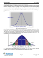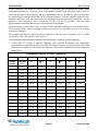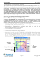
1
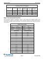
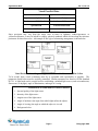
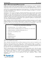
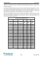
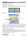
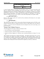
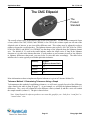
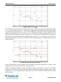
Vol. 17, No. 12
Insight on Color
Establishing Instrumental Color Difference Tolerances for
Your Products
Overview
Color is a very important aspect of products for consumers. The appearance of a product is perceived
(often correctly) to be related to its quality. This is true in almost all industries. From cookies to vinyl
siding, customer buying decisions are often based on product color, making it important to bakers and
extruders alike.
The color of a product may be judged generally to be “acceptable” or “unsatisfactory,” or it may be
judged in more detail to be “too light,” “too red,” or “too blue.” Such judgments can be made visually
or instrumentally based on a perceived difference between an ideal product standard and a sample.
When this difference is quantified, tolerances can be established.
Tolerances are limits within which a product is considered acceptable. Any product falling outside the
tolerances is unacceptable. Having good tolerances in place for each product allows you to make quick
and easy pass/fail or ship/don’t ship decisions. When tolerances are established instrumentally, they
may be expressed in any of the color scales or indices available with the instrument. In order to set
tolerances, an ideal or close-to-ideal product standard is required, as well as a variety of products that
have already been determined to be acceptable or unacceptable.
There are two levels of visual color differences that are used to establish color tolerances:
•
Minimum perceptible difference, which defines a just-noticeable difference between standard and
sample.
•
Maximum acceptable difference, which is the largest acceptable difference between standard and
sample.
Page 1
©Copyright 2008
Applications Note
Vol. 17, No. 12
Perceptible vs. Acceptable Differences
Manufacturers are generally concerned about the maximum acceptable color difference rather than a
minimum perceptible difference, and color tolerances are usually based on the maximum acceptable
difference. Any difference larger than that would cause the sample to be rejected.
In the end, agreement between the buyer and seller on acceptability criteria is necessary for establishing
product color tolerances and purchasing specifications.
A step-by-step process for establishing color difference tolerances is outlined in the rest of this
Applications Note.
Step I. Establish a Standard
The first step in implementing a tolerancing program is to establish a standard that represents the ideal
color for a particular product. In theory, the established manufacturing process should be capable of
producing this color the majority of the time.
Tolerances should be established separately for each product color, so you will need a product standard
for each color. It is normal to have difference tolerances for different colors. (It is also typical to find
that your tolerances must be tighter to provide acceptable results for darker colors and lower-chroma
colors.)
In a customer/vendor relationship, the standard representing the target color may be submitted by a
designer or customer. This submission is then matched by the vendor’s manufacturing process and
returned to the customer for approval. This begins the process of color communication.
On the other hand, when the color evaluation is being driven by internal quality concerns, it is most
effective to use a standard that represents the process average. This can be accomplished by selecting a
physical specimen from the center of the population or by averaging the measured results of a group of
specimens to determine a numeric mean. An example of determining a colorimetric mean is shown
below. Many HunterLab products (ColorFlex, DP-9000, EasyMatch Coatings, EasyMatch OnLine,
EasyMatch QC, MiniScan XE Plus, Universal Software) can automatically average samples for you.
Page 2
©Copyright 2008
Applications Note
Vol. 17, No. 12
Use of the Mean for Establishing a
Standard
Sample ID
L*
a*
b*
1
20.22
0.64
-11.22
2
20.70
0.66
-11.02
3
20.73
0.61
-10.99
4
20.38
0.60
-10.82
5
20.75
0.49
-10.62
6
20.37
0.50
-10.43
7
19.99
0.54
-11.20
8
20.15
0.52
-10.81
9
20.29
0.59
-10.55
10
20.48
0.57
-11.22
11
20.50
0.64
-10.72
12
19.87
0.70
-11.02
13
20.81
0.59
-11.22
14
20.31
0.53
-11.18
15
20.56
0.61
-10.57
Average
20.41
0.59
-10.91
Care should be taken to preserve the color of physical standards by minimizing the influence of light,
temperature, contamination, and other aging factors. A system may be established whereby duplicate
standards are created and stored until needed. The amount of change in a current, or “working,”
standard over time can be determined by comparing it to a stored, and theoretically pristine, duplicate.
If an instrument is being used to measure color, the current instrumental reading for the standard can be
compared to the previously assigned values. As suggested by the SAE J1545 Recommended Practice, if
a working standard has deviated by the greater of 0.2 color difference units in ∆L*∆a*∆b* or
∆L*∆C*∆H* or 0.1 times the tolerance range, the standard should be carefully evaluated and possibly
replaced with a back-up. The worksheet below details an example evaluation of such a standard.
Page 3
©Copyright 2008
Applications Note
Vol. 17, No. 12
Verifying a Physical Standard
Color Scale
Tolerances
Pass/Fail
Criteria
Assigned
Values
Current
Values
Difference
(Delta)
L*
±0.50
0.20
24.81
24.87
0.06 PASS
a*
±0.40
0.20
-5.16
-5.18
-0.02 PASS
b*
±0.30
0.20
-4.61
-4.43
0.18 PASS
This standard does not need to be replaced.
Step II. Visually Evaluate Pass/Fail
Once the product standard is established, a “pass” or “fail” rating can be assigned visually to any
specimen that is compared to that standard. Results should be reported in a fashion similar to those
shown below, including complete information on the particular conditions under which the specimens
were evaluated.
Visual Pass/Fail Data
Date:
4/12/05
Operator:
KSS
Apparatus:
Light Booth
Lamp:
Daylight
Product:
PF11280-408
Standard:
11280
Specimen ID
Pass/Fail Indication
11287
Pass
11295
Pass
11211
Pass
11213
Pass
11213
Pass
11220
Pass
11241
Pass
11242
Pass
11264
Pass
11266
Fail
11272
Fail
11395
Fail
11411
Pass
11415
Fail
Page 4
©Copyright 2008
Applications Note
Vol. 17, No. 12
Visual Pass/Fail Data
Date:
4/12/05
Operator:
KSS
Apparatus:
Light Booth
Lamp:
Daylight
Product:
PF11280-408
Standard:
11280
Specimen ID
Pass/Fail Indication
11111
Fail
Since specimens may vary from the target color in terms of lightness, redness/greenness, or
yellowness/blueness, it may be helpful to employ physical standards which deviate along the tolerance
perimeters for these three axes. An example of this type of tolerancing arrangement is shown below.
Visual Deviations from Target in Lightness/Darkness, Red/Green, and Blue/Yellow
To be useful, these visual evaluations must be as repeatable and reproducible as possible. The
parameters listed below must be carefully controlled. Similar parameters are listed in ASTM Standard
D1729. A light booth can be a useful tool for establishing a standard light source (such as incandescent,
fluorescent, or daylight), angle of illumination, and angle of viewing.
Conditions to be Controlled for Visual Evaluation
1. Spectral quality of the light source
2. Intensity of the light source
3. Angular size of the light source
4. Angle of incidence (the angle from which light strikes the object)
5. Angle of viewing (the angle at which the object is viewed)
6. Background color.
Page 5
©Copyright 2008
Applications Note
Vol. 17, No. 12
Step III. Make Instrumental Measurements
Modern color measuring instruments (spectrophotometers and colorimeters) use the CIE colorimetric
mathematical model to relate the human perception of color to instrumental response. Colorimetric
scales such as CIE L*a*b* and CIE L*C*h can be derived from this mathematical model to serve as
useful tools in communicating and quantifying color and appearance. The numbers obtained describe
the nature and magnitude of the difference in color between standard and sample in a way that is
meaningful to a human observer.
Instruments not only provide an objective, numerical measurement system, but they can also often
discriminate or “see” small color differences better than the average human observer and can do so
repeatably. In other words, instruments are more accurate and more repeatable than humans. Another
recognized advantage to using instrumentation is the agreement on specimen readings between different
instruments, which is better than the agreement between visual assessments by two different human
observers. This function, known as reproducibility, easily expands the capability for communication of
color between different manufacturing facilities.
When comparing results for different specimens measured on different instruments, specific sample
handling techniques and instrumental settings should be defined and used. Adherence to a defined
method will reduce the error associated with sample presentation and instrumentation. Some of the
parameters to be considered and standardized in test method development are listed below.
Criteria for Color Measurement Methodology
•
Instrument geometry: 45°/0° or diffuse/8° (sphere)
•
Sample preparation, including taking opacity, translucency, etc. into account
•
Sample presentation, including instrument port size, etc.
•
Color scale or color difference scale
•
Illuminant
•
Standard observer
•
Standardization mode
•
Sample averaging.
The recommended practices of various professional trade associations (such as ASTM, TAPPI, and
AATCC) are available in the literature.
When comparing measurements made on different instruments, the best results are obtained for color
differences when the instrument group contains units of similar geometrical design. For instance, it
would not be advisable to compare results obtained on a 45°/0° instrument to those obtained using a
diffuse/8° instrument. For recommendations of ways to maximize inter-instrument agreement, refer to
the Applications Note titled “Maximizing Inter-instrument Agreement.”
When it is important that two or more instruments of similar design read the “same” values for a group
of specimens, the technique of hitch standardization may be employed. This process involves naming
one instrument as the reference, or “master,” unit and mathematically adjusting the secondary, or
“slave,” units to match. In this way, two or more instruments can be “hitched” together. For more
information on this process, see the Applications Note titled “HunterLab’s Guide to Hitch
Standardization.”
Page 6
©Copyright 2008
Applications Note
Vol. 17, No. 12
Instrument diagnostics provided by the instrument manufacturer should be run on a regular basis.
Adherence to a schedule will ensure confidence in the measurements and allow early detection of
instrumental problems.
Once the instrument and method are in place, it is time to gather and read a group of samples. To be
most effective, this group should be large enough to provide some statistical credibility (i.e., twenty or
more samples) and should include samples that pass, as well as samples that fail when visually rated.
Specimens that are unacceptable assist in finding the numerical tolerance boundaries. To verify and
refine the initial product tolerances, expand the data base by collecting more samples.
Next, rate the acceptability (in terms of pass or fail) of each sample by visually comparing it to the
physical product standard as described in Step II (if you haven’t already). Then, measure each of these
samples on the instrument and determine its color difference relative to the product standard. And
example data summary is shown below.
Visual and Instrumental Data
1
2
3
4
5
6
Sample
Number
Specimen
ID
Visual
Pass/Fail
∆L*
∆a*
∆b*
1
11287
Pass
0.23
0.01
0.09
2
11295
Pass
0.46
0.03
-0.08
3
11211
Pass
-0.15
0.12
0.05
4
11213
Pass
-0.01
-0.07
0.04
5
11216
Pass
-0.03
-0.14
0.18
6
11220
Pass
0.12
0.09
0.15
7
11241
Pass
-0.20
-0.18
-0.11
8
11242
Pass
-0.37
0.15
-0.23
9
11259
Pass
-0.49
-0.19
0.02
10
11264
Pass
0.46
0.13
0.15
11
11266
Fail
0.56
0.26
0.30
12
11272
Fail
-0.61
-0.24
0.04
13
11395
Fail
-0.78
-0.27
-0.21
14
11411
Pass
-0.34
-0.04
0.16
15
11415
Fail
-0.86
-0.45
-0.17
16
11111
Fail
1.25
0.44
0.25
Page 7
©Copyright 2008
Applications Note
Vol. 17, No. 12
Step IV. Establish the Tolerances
There are several types of tolerances you may establish and several methods for doing so, which are
outlined below.
Tolerance Type 1: Rectangular Tolerances
Rectangular tolerances are the simplest type of tolerances and are shown in a form similar to the
example given below. All three components of the color scale (such as L*, a*, and b* or L, a, and b)
should be toleranced.
Color Tolerances for the RED 3645 Standard
L* (D65/10°)
43.48 ± 0.50
a* (D65/10°)
45.45 ± 0.50
b* (D65/10°)
27.15 ± 0.50
These tolerances are “rectangular,” because when plotted on a color plot, they are expressed as a
rectangle.
L* tolerance
b* tolerance
a* tolerance
Sometimes 0.2 CIE L*a*b* units is quoted as an “approximate visual difference limit,” so it may be
tempting to use such a number for your rectangular tolerances. In general, however, tolerances should
be based on visual assessment using measurements of acceptable and unacceptable samples and an
“ideal” product standard, as the 0.2 unit difference will likely be too tight for most applications,
resulting in discard or rework of product that might actually have been acceptable to the customer.
Rectangular tolerances may be established using Tolerance Method 1, Method 2, or even Method 3b
described below.
Tolerance Type 2: Single-Number Tolerances
If your customer cares only about one component of the color scale (such as L, or lightness), or asks for
readings only in a particular index (such as Yellowness Index), it is acceptable to establish a tolerance
only for the parameter of interest. This tolerance may be established using Method 1, Method 2, or even
Method 3b (if the parameter of interest is a component of the color scale).
An example single-number tolerance is shown below.
Page 8
©Copyright 2008
Applications Note
Vol. 17, No. 12
Color Tolerance for the WHITE BASE
Standard
YI E313 (C/2°)
<5 units
A word of caution, however, concerning total color difference values. It is not wise to use ∆E or ∆E*
alone as a tolerance if all the components of the color scale are truly of interest. This is because,
although the product may be perfectly acceptable when the color difference is spread out over all three
dimensions (L, a, and b or L*, a*, and b*), if the difference is concentrated on one of the dimensions, it
may be obviously unacceptable. For example, if a given tolerance is 1 ∆E (Hunter L, a, b) unit, the
difference could be 0.57 for L, 0.57 for a, and 0.57 for b, and would probably be acceptable visually.
∆E = 0.57 2 + 0.57 2 + 0.57 2 = 1 .
However, if the sample is perfect for L and b but off (yet within the ∆E tolerance) for a, the sample
looks very unacceptable.
∆E = 0.0 2 + 1.0 2 + 0.0 2 = 1 .
This caution does not apply to the ∆E values used in elliptical tolerancing (such as ∆E CMC), as the
elliptical tolerancing systems are designed specifically to provide a single-number total color difference
tolerance. See the next section for information on how the elliptical scales can be used to help you set
pass/fail tolerances.
Tolerance Type 3: Elliptical Tolerances
The following general rules apply to human assessments of color:
•
Hue (h) differences are most objectionable.
•
Humans will tolerate a little more difference in chroma (C*) than in hue (h).
•
Humans will tolerate lightness (L*) differences more easily than differences in chroma (C*) or hue
(h).
These principles form the basis for elliptical tolerancing. The elliptical tolerancing scales are CMC,
CIE94, DIN99, and CIE2000 (all available in EasyMatch QC and EasyMatch OnLine; consult your
User’s Manual for availability with other products), and they operate on the principle that the limit of the
region of color space surrounding a product standard for which color differences are not visually
detectable forms an ellipsoid with axes in the direction of lightness (l), chroma (c), and hue (h).
Page 9
©Copyright 2008
Applications Note
Vol. 17, No. 12
The CMC Ellipsoid
The
Product
Standard
The overall volume (size) of the ellipse is the overall color tolerance. For the default commercial factor
of one (called cf for CMC, DIN99, and CIE2000, kv for CIE94), this volume equals one ∆E unit of the
elliptical scale of interest, or one just-visible-difference unit. This volume may be adjusted in order to
tighten or loosen the overall tolerance. The lightness:chroma ratio (called l:c for CMC, kl:kc for CIE94,
ke:kch for DIN99, and KL:KC for CIE2000) sets the shape of the ellipsoid along the lightness-chroma
axis. The default of 2:1 used in the textile industry makes the ellipse twice as long in the lightness
direction as it is wide in the chroma direction. If your product or your customer is more or less sensitive
to lightness differences than usual, you may lower or raise this ratio accordingly. The table below
indicates the l:c ratios typically used within particular industries.
Industry
Typical
lightness:chroma Ratio
Coatings
1:1
Plastics
1.3:1
Textiles
2:1
More information on how to implement elliptical tolerances is given in Tolerance Method 3a.
Tolerance Method 1: Determining Tolerances Using a Graph
To demonstrate this method of establishing tolerances, we will create a graph for each of the difference
values listed in the table in Step III (page 7). As an example, we will plot the lightness/darkness (L*)
differences. The y-axis will contain the color difference values (column 4) and the x-axis will contain
the sample number (column 1). The plot is shown below.
Note: Some HunterLab software products can create this graph for you. Look for a “trend plot” or
“control chart” view.
Page 10
©Copyright 2008
Applications Note
Vol. 17, No. 12
Sample Number Versus ∆L*
Next, add the visual pass/fail data by labeling each sample as passing (no label) or failing (labeled with
an “F”) using the table’s column 3. As shown below, upper and lower boundary lines can then be drawn
to separate the graph into three areas. The lower rectangle (below the lower red line) represents all the
samples that fall outside the lower tolerance (i.e., are too dark), the middle rectangle (between the red
lines) represents all samples which are acceptable for L*, and the upper rectangle (above the upper red
line) represents all the samples that fall outside the upper tolerance (i.e., are too light.) You can see that
both the upper and lower L* limits occur at about 0.5 L* from the standard. ±0.5 would be used as your
starting tolerance.
Pass/Fail Labels and Tolerance Limits
Next, you should make a similar graph for the remaining color difference parameters, a* and b*, using
columns 1 and 5 and 1 and 6, respectively, of the data table.
Using this graphing technique, twenty well-chosen samples will provide a good set of starting
tolerances. Data on future specimens should be added to the graph to check the ongoing validity of the
specifications. As the sampling number approaches 50 or more, confidence in the tolerances should
greatly increase.
Page 11
©Copyright 2008
Applications Note
Vol. 17, No. 12
Tolerance Method 2: Determining Tolerances Using Statistics
Much of the data obtained in an ongoing production process will assume the shape of a bell curve when
plotted as a frequency polygon. This shape is more commonly referred to as the normal distribution
curve and is useful when studying color difference values. Certain statistical assumptions can be made
about the normal curve that are useful in describing the population. One of these statistical properties,
the standard deviation, helps to describe the distribution of the measurements about the average, or
population mean.
MEAN
FREQUENCY
STANDARD DEVIATIONS
The Normal Distribution Curve
Color difference measurements are plotted on the x-axis and their corresponding frequencies are plotted
on the y-axis. The x-axis can be divided into equal parts called standard deviation or sigma (σ) units.
The value given to the standard deviation at the center of the curve represents 100% of the measurement
in question. For each standard deviation, a portion of the total area is represented. At the level of ±3σ,
approximately 99.7% of the population is covered.
Population Distributions for the Normal Curve
It is generally agreed that tolerance limits can be set at the ±3σ level over the process range for
acceptable values. This concept is based on statistical process control (SPC) studies.
Page 12
©Copyright 2008
Applications Note
Vol. 17, No. 12
Process capability is the degree to which a process is consistently able to manufacture product within
established specifications. “Process” refers to the product variables being measured, such as color, as
well as the procedures, the machinery, and the workmanship involved. Results are usually expressed as
the proportion or percent of product that will be within the tolerance. Process capability studies are SPC
techniques which are valid only after statistical control has been determined and established. For the
purposes of this Applications Note, a discussion of SPC will not be provided. However, more
information can be found in the literature referenced in the bibliography.
In practical terms, a process that is not “in control” and is constantly shifting does not lend itself well to
fixed tolerance limits. Process capability studies are needed to set tolerances, as well as to evaluate
current specifications.
The accepted criterion for long-term process capability is that the process function is 99.7% within
specification. This 99.7% refers to the ±3σ level.
To determine the upper and lower tolerance limits statistically, complete the following steps:
1. Collect data on a group of samples, including visual pass/fail information and instrumental
measurements (as described in Steps II and III). Determine the mean colorimetric values and, using
this mean as a standard, calculate the color difference between this standard and all the samples as
shown below.
Colorimetric Data on Cracker Production
1
2
3
4
5
6
7
8
Sample
Number
Specimen
ID
L*
∆L*
a*
∆a*
b*
∆b*
1
GG
50.95
-6.40
15.46
2.94
37.37
-3.50
2
AA
51.21
-6.14
15.54
3.02
38.75
-2.12
3
NN
52.28
-5.07
14.88
2.36
37.75
-3.12
4
MM
53.01
-4.34
14.29
1.77
37.45
-3.42
5
OO
54.01
-3.34
14.52
2.00
41.44
0.57
6
PP
54.15
-3.20
14.74
2.22
40.23
-0.64
7
BB
54.89
-2.46
13.72
1.20
39.52
-1.35
8
B1
54.98
-2.37
14.07
1.55
41.92
1.05
9
RR
55.27
-2.08
13.46
0.94
39.99
-0.88
10
QQ
55.72
-1.63
13.82
1.30
41.24
0.37
11
JJ
56.32
-1.03
13.15
0.63
40.62
-0.25
12
SS
56.90
-0.45
13.22
0.70
40.04
-0.83
13
KK
57.02
-0.33
12.86
0.34
40.39
-0.48
14
TT
57.05
-0.30
12.53
0.01
39.53
-1.34
15
DD
57.10
-0.25
13.00
0.48
41.91
1.04
Page 13
©Copyright 2008
Applications Note
Vol. 17, No. 12
Colorimetric Data on Cracker Production
1
2
3
4
5
6
7
8
Sample
Number
Specimen
ID
L*
∆L*
a*
∆a*
b*
∆b*
16
II
57.12
-0.23
13.16
0.64
40.75
-0.12
17
VV
57.61
0.26
12.67
0.15
43.72
2.85
18
CC
57.71
0.36
12.74
0.22
41.08
0.21
19
EE
58.19
0.84
12.18
-0.34
41.42
0.55
20
HH
59.14
1.79
11.99
-0.53
41.30
0.43
21
ZZ
59.26
1.91
11.86
-0.66
41.01
0.14
22
LL
59.98
2.63
11.16
-1.36
40.82
-0.05
23
C1
60.08
2.73
11.08
-1.44
43.46
2.59
24
YY
61.10
3.75
10.33
-2.19
43.49
2.62
25
WW
62.65
5.30
9.09
-3.43
42.14
1.27
26
XX
64.01
6.66
8.41
-4.11
42.37
1.50
27
A1
64.07
6.72
8.22
-4.30
42.17
1.30
28
UU
64.10
6.75
8.45
-4.07
42.48
1.61
Mean (Standard)
57.35
12.52
40.87
2. Determine the standard deviation for each color difference parameter and summarize the data as
shown below.
Summary Statistics for Crackers
L*
Number of Samples
28
a*
28
b*
28
Minimum Value
50.95
8.22
37.37
Maximum Value
64.10
15.54
43.72
Range
13.15
7.32
6.35
Mean
57.35
12.52
40.87
Standard Deviation
3.67
2.08
1.69
3. Then, assuming a normal distribution, plot the data for each colorimetric value (Microsoft Excel can
do this) and view the shape of the distribution and the location of the 3σ level. An example for ∆L*
is shown below.
Page 14
©Copyright 2008
Applications Note
Vol. 17, No. 12
dL* Distribution
20
15
Count
10
5
0
-15
-10
-3σ
-5
0
5
-5
dL*
10
15
3σ
4. Assume that the desired specification limits are equal to ±3σ and find the tolerance limits for each
color scale parameter using the following equations. The example shown is for L*.
For absolute tolerances:
Lower Limit = -3σ + Mean
Lower Limit = (-3*3.67) + 57.35
Lower Limit = 46.34
Upper Limit = 3σ + Mean
Upper Limit = (3*3.67) + 57.35
Upper Limit = 68.36
For difference tolerances (recommended):
Lower Difference Limit = -3σ
Lower Difference Limit = -3*3.67
Lower Difference Limit = -11.01
Upper Difference Limit = 3σ
Upper Difference Limit = 3*3.67
Upper Difference Limit = 11.01
As additional samples are read, they should be added to the distribution plot to test the effectiveness of
the 3σ tolerances. If the ends of the 3σ range begin to include out-of-specification product, the tolerance
should be recalculated to reduce the range and the standard deviation of the in-tolerance samples. This
will better exclude the out-of-tolerance samples from the specification.
Another approach to solidifying tolerances is to assess the capability of the process to manufacture
product within the set specifications. Information on completing a process capability study is available
in the literature and involves using a formula similar to the one already presented. The aim would be to
substitute in the current tolerances and solve for the number of standard deviations needed to include the
in-tolerance samples. The result would predict the percentage of the population that could be produced
within tolerance using the current manufacturing process and specifications.
Page 15
©Copyright 2008
Applications Note
Vol. 17, No. 12
Tolerance Method 3a: Using Elliptical Tolerances
This section describes how to actually implement the elliptical tolerances described in Tolerance Type 3.
Ellipsoidal volumes are thought to more accurately describe human perceptibility limits than rectangular
tolerance boxes. By definition, any sample that falls within the ellipsoid (and the ∆E limit chosen for
the scale being used) is acceptable for the standard at its center and any sample that is outside the
ellipsoid (and the ∆E limit chosen for the scale being used) is unacceptable. Thus, assigning tolerances
for a product standard using elliptical tolerancing is as simple as reading the standard, choosing the
elliptical scale for use, and setting the lightness: chroma ratio and commercial factor (beginning with
industry defaults and adjusting as needed using read samples). Then, samples outside the ∆E limit will
fail and samples inside the ∆E limit will pass.
Refer to your User’s Manual for more information on elliptical tolerances.
Tolerance Method 3b: Using Automatic Tolerancing
In HunterLab’s EasyMatch QC, CMC autotolerancing can be used to automatically fit a CMC ellipsoid
to a standard and to calculate CIE L*a*b*, CIEL*C*h, or Hunter L, a, b rectangular tolerances for that
standard based on the size and shape of the ellipsoid. Once the ideal product standard is read, the
parameters for the automatic tolerancing can be set through the software, as follows:
•
Color Scale: scale under which you would like the automatically-generated tolerances to be
expressed (CIE L*a*b*, CIEL*C*h, or Hunter L, a, b)
•
Illuminant/Observer: illuminant/observer combination under which you would like the
automatically-generated tolerances to be expressed
•
l:c ratio: as described in Tolerance Method 3a.
•
Commercial factor: as described in Tolerance Method 3a.
•
Auto tolerance Correction factor: the 0.75 default value in EasyMatch QC estimates the percentage
of the tolerance box that is taken up by the CMC ellipsoid (excluding the 25% of the box volume
that does not overlap with the ellipsoid). This value may be adjusted to tighten or loosen the
tolerance, as desired. A value of one would use the entire volume of the tolerance box, including
those areas outside the CMC ellipsoid, as shown below.
The elliptical
tolerances
The
rectangular
tolerances
Example of an area of the
tolerance box outside (and
not overlapping with) the
ellipsoid
Page 16
©Copyright 2008
Applications Note
Vol. 17, No. 12
After all parameters are set, the rectangular tolerances are automatically generated and used by the
software for samples that are compared to this product standard.
Refer to the EasyMatch QC User’s Manual for more information on using the automatic tolerancing
feature of that software package.
CMC autotolerancing can also be used within HunterLab’s ColorFlex and MiniScan XE Plus firmware
to automatically fit a CMC ellipsoid to a standard and to calculate ∆L*∆C*∆H* rectangular tolerances
for that standard based on the size and shape of the ellipsoid.
In the product setup select the L*a*b* color scale, ∆L* ∆C* ∆H* color difference scale, and ∆Ec index
difference. Enter the desired commercial factor (cf) and the l:c ratio as described in Tolerance Method
3a. You must also select a “PHYSICAL” type standard and read your product standard into the setup.
After the standard is read, the automatically-generated ∆L*, ∆C*, ∆H* tolerances are entered into and
used with this product setup unless they are manually altered or another product standard is read into
this setup.
Refer to your ColorFlex or MiniScan XE Plus User’s Guide for more information on using the automatic
tolerancing feature of the instrument.
Bibliography
AATCC Test Method 173, “CMC: Calculation of Small Color Differences for Acceptability,” American
Association of Textile Chemists and Colorists, Research Triangle Park, North Carolina, www.aatcc.org.
ASTM D1729, “Standard Practice for Visual Appraisal of Colors and Color Differences of DiffuselyIlluminated Opaque Materials,” ASTM International, West Conshohocken, Pennsylvania,
www.astm.org.
ASTM D3134, “Standard Practice for Establishing Color and Gloss Tolerances,” ASTM International,
West Conshohocken, Pennsylvania, www.astm.org.
Hunter, Richard S. and Harold, Richard W., The Measurement of Appearance, New York: John Wiley &
Sons, 1987, www.hunterlab.com.
“HunterLab’s Guide to Hitch Standardization,” Applications Note, HunterLab, September 1998.
“Maximizing Inter-instrument Agreement,” Applications Note, HunterLab, June 2005.
Recommended Practice J1545, “Instrumental Color Difference Measurement for Exterior Finishes,
Textiles, and Colored Trim,” SAE International, Warrendale, Pennsylvania, www.sae.org.
For Additional Information Contact:
Technical Services Department
Hunter Associates Laboratory, Inc.
11491 Sunset Hills Road
Reston, Virginia 20190
Telephone: 703-471-6870
FAX: 703-471-4237
www.hunterlab.com
03/08
Page 17
©Copyright 2008