Download Swytink-Binnema_Nigel - UWSpace

Digital Tuft Flow Visualisation of
Wind Turbine Blade Stall
by
Nigel Swytink-Binnema
A thesis
presented to the University of Waterloo
in fulfillment of the
thesis requirement for the degree of
Master of Applied Science
in
Mechanical Engineering
Waterloo, Ontario, Canada, 2014
c Nigel Swytink-Binnema 2014
I hereby declare that I am the sole author of this thesis. This is a true copy of the thesis,
including any required final revisions, as accepted by my examiners.
I understand that my thesis may be made electronically available to the public.
ii
Abstract
Wind turbines installed in the open atmosphere experience much more complex and
highly-varying flow than their counterparts in wind tunnels or numerical simulations. In
particular, aerodynamic stall—which occurs often on stall-regulated wind turbines in such
variable flow conditions—can affect both wind turbine blade lifespan and noise generation.
A field test site was therefore installed at the outer limits of the city of Waterloo, Ontario
to study a small-scale 30 kW stall-regulated wind turbine.
Experimental equipment was installed to monitor parameters such as wind speed and
direction, electrical power output, blade pitch angle, rotor rotational speed, and wind
turbine yaw orientation. Extensive hardware and software was developed and installed to
wirelessly collect data from all instrumentation. Tufts and a remote-operated camera were
also installed on one of the two blades of the 10 m diameter horizontal-axis turbine.
In a variation on the tuft flow visualisation technique, video files were analysed using a
R
novel digital image processing code. The code was developed in MATLAB
to calculate
the fraction of the blade which was stalled by determining the position and angle of each
tuft in every video frame. The algorithm was able to locate on average 85% of the visible
tufts and correctly tagged those which were stalled with a bias of only −5% compared to
the typical manual method. When the algorithm was applied to 7 h of tuft video at the
outboard 40% of the blade, the total average fraction of stalled tufts varied from 5% at
5 m/s to 40% at 21 m/s. This trend was expected for the stall-regulated design since, as
the wind speed is increased, the stall progresses from inboard to outboard regions and from
trailing edge to leading edge.
The 7 h time period represents at least a two order-of-magnitude increase compared
with time periods analysed using previous manual methods. This work has demonstrated
a digital implementation of tuft flow visualisation which lends statistical validity (through
long-time-period averaging) to a common tool for researching wind turbine stall. The
speed and ease with which the tuft method can be implemented, combined with the high
cost per energy of small-scale wind turbines, suggest that this digital algorithm is a highly
beneficial tool for future studies.
iii
Acknowledgements
I would like to sincerely thank the following people for their support throughout the
past three years. This work has my name on it but it would have been impossible without
them.
Firstly, my supervisor Professor David Johnson. He provided direction and guidance
when I needed it in my thesis work and when other issues arose. The experience he provided
me with over the past three years went far beyond the technical nature of this writing.
Secondly, I extend a huge thank you to Curtis Knischewsky for hundreds of hours of
engineering design, building, and installation of equipment. Nicholas Tam’s expertise with
the wireless networking on site and willingness to offer support on evenings and weekends
made my work that much less stressful. I would also like to thank the other graduate
students in our group for their input and support over the past few years: Ahmed Abdelrahman, Kobra Gharali, Faegheh Ghorbani Shohrat, Rifki Adi Nugroho, and Rizwana
Amin.
All engineers know we would be nowhere without the knowledge and skills of technicians. In my case, the technicians Jason Benninger, Neil Griffett, Andy Barber, and Terry
Ridgway at the University of Waterloo have been invaluable.
The support of my parents and sister back home was essential in both the day-to-day
and the holidays. Here in Waterloo, my aunt and uncle were wonderful for adopting me
into their life and for all the free meals.
Thanks to Ann Sychterz, Sara VanderVies, Kevin Purbhoo, Richard Gu, Andrew Ikert,
Naomi Mahaffy, Holly Neatby, and Nicholas Tam, I have had many great friendships,
debates about life and engineering, dancing, bike rides, and dinner parties. I look forward
to more of the same, wherever life takes us.
Finally, a thank you is in order for co-op students Brandon Coles, Jennifer Chan, Daniel
Lizewski, Daryn Huang, Alastair Tauro, Daniel Dworakowski and over half a dozen others
who helped me with various projects over the past couple years.
iv
Dedication
This work is dedicated to all who visualise fluid flow, whether on the street or in the
lab. Fluid motion remains mysterious and invisible until you choose to see it.
v
Table of Contents
List of Figures
xii
List of Tables
xvi
Nomenclature
xvii
Acronyms
xx
1 Introduction
1
1.1
Horizontal-axis wind turbines . . . . . . . . . . . . . . . . . . . . . . . . .
1
1.2
Motivation . . . . . . . . . . . . . . . . . . . . . . . . . . . . . . . . . . . .
4
1.3
Project overview . . . . . . . . . . . . . . . . . . . . . . . . . . . . . . . .
4
1.4
Outline of thesis . . . . . . . . . . . . . . . . . . . . . . . . . . . . . . . . .
6
2 Background
2.1
2.2
7
Theory of aerodynamic lift and drag . . . . . . . . . . . . . . . . . . . . .
7
2.1.1
Two-dimensional airfoils . . . . . . . . . . . . . . . . . . . . . . . .
7
2.1.2
Three-dimensional wings . . . . . . . . . . . . . . . . . . . . . . . .
11
Aerodynamics of wind turbines . . . . . . . . . . . . . . . . . . . . . . . .
11
2.2.1
A blade element model . . . . . . . . . . . . . . . . . . . . . . . . .
13
2.2.2
Wind turbine power output . . . . . . . . . . . . . . . . . . . . . .
15
2.2.3
Comparing wind turbine performance . . . . . . . . . . . . . . . . .
17
vi
2.2.4
2.3
2.4
The nature of the wind . . . . . . . . . . . . . . . . . . . . . . . . .
19
Tuft flow visualisation . . . . . . . . . . . . . . . . . . . . . . . . . . . . .
20
2.3.1
Tuft methods . . . . . . . . . . . . . . . . . . . . . . . . . . . . . .
20
2.3.2
Tufts on wind turbines . . . . . . . . . . . . . . . . . . . . . . . . .
22
Studies of wind turbine stall . . . . . . . . . . . . . . . . . . . . . . . . . .
24
2.4.1
Pederson and Madsen tuft study
. . . . . . . . . . . . . . . . . . .
24
2.4.2
Eggleston and Starcher’s wind turbine comparison . . . . . . . . . .
24
2.4.3
Haans et al. micro-scale turbine study . . . . . . . . . . . . . . . .
27
2.4.4
Maeda and Kawabuchi study . . . . . . . . . . . . . . . . . . . . .
29
2.4.5
The NREL experiments . . . . . . . . . . . . . . . . . . . . . . . .
30
2.4.5.1
The Unsteady Aerodynamics Experiment . . . . . . . . .
30
2.4.5.2
Other derived studies
32
. . . . . . . . . . . . . . . . . . . .
3 Experimental Setup
35
3.1
Overview of the test site . . . . . . . . . . . . . . . . . . . . . . . . . . . .
35
3.2
The wind turbine . . . . . . . . . . . . . . . . . . . . . . . . . . . . . . . .
37
3.3
Instrumentation . . . . . . . . . . . . . . . . . . . . . . . . . . . . . . . . .
41
3.3.1
Camera . . . . . . . . . . . . . . . . . . . . . . . . . . . . . . . . .
42
3.3.2
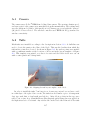
Tufts . . . . . . . . . . . . . . . . . . . . . . . . . . . . . . . . . . .
43
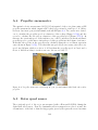
3.3.3
Blade pitch angle . . . . . . . . . . . . . . . . . . . . . . . . . . . .
44
3.3.4
Hub wind speed . . . . . . . . . . . . . . . . . . . . . . . . . . . . .
45
3.3.5
Rotor speed . . . . . . . . . . . . . . . . . . . . . . . . . . . . . . .
45
3.3.6
Yaw orientation . . . . . . . . . . . . . . . . . . . . . . . . . . . . .
47
3.3.7
Velocity at wind turbine tower . . . . . . . . . . . . . . . . . . . . .
48
3.3.8
Electrical power and control . . . . . . . . . . . . . . . . . . . . . .
49
3.3.9
The meteorological tower . . . . . . . . . . . . . . . . . . . . . . . .
51
Data logging . . . . . . . . . . . . . . . . . . . . . . . . . . . . . . . . . . .
53
3.4.1
53
3.4
Base computer . . . . . . . . . . . . . . . . . . . . . . . . . . . . .
vii
3.5
3.4.2
Camera . . . . . . . . . . . . . . . . . . . . . . . . . . . . . . . . .
54
3.4.3
Meteorological tower . . . . . . . . . . . . . . . . . . . . . . . . . .
55
3.4.4
G30 controller . . . . . . . . . . . . . . . . . . . . . . . . . . . . . .
55
3.4.5
NI data loggers . . . . . . . . . . . . . . . . . . . . . . . . . . . . .
56
3.4.6
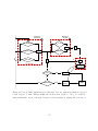
The wireless network . . . . . . . . . . . . . . . . . . . . . . . . . .
57
3.4.7
Data acquisition code . . . . . . . . . . . . . . . . . . . . . . . . . .
59
Summary . . . . . . . . . . . . . . . . . . . . . . . . . . . . . . . . . . . .
60
4 The Algorithm
63
4.1
Video file preparation . . . . . . . . . . . . . . . . . . . . . . . . . . . . . .
63
4.2
Procedure . . . . . . . . . . . . . . . . . . . . . . . . . . . . . . . . . . . .
65
4.2.1
Input images . . . . . . . . . . . . . . . . . . . . . . . . . . . . . .
65
4.2.2
Extract foreground . . . . . . . . . . . . . . . . . . . . . . . . . . .
69
4.2.3
Locate tufts . . . . . . . . . . . . . . . . . . . . . . . . . . . . . . .
70
4.2.4
Locate stalled tufts . . . . . . . . . . . . . . . . . . . . . . . . . . .
73
4.2.4.1
Tuft threshold stall angle . . . . . . . . . . . . . . . . . .
74
4.2.5
The stall fraction . . . . . . . . . . . . . . . . . . . . . . . . . . . .
76
4.2.6
Summary of algorithm . . . . . . . . . . . . . . . . . . . . . . . . .
78
Algorithm validation . . . . . . . . . . . . . . . . . . . . . . . . . . . . . .
79
4.3.1
Stall criteria . . . . . . . . . . . . . . . . . . . . . . . . . . . . . . .
79
4.3.2
Algorithm bias . . . . . . . . . . . . . . . . . . . . . . . . . . . . .
80
Algorithm characteristics . . . . . . . . . . . . . . . . . . . . . . . . . . . .
83
4.4.1
Overview . . . . . . . . . . . . . . . . . . . . . . . . . . . . . . . .
84
4.4.2
Effect of constraints
. . . . . . . . . . . . . . . . . . . . . . . . . .
84
4.4.2.1
Accuracy . . . . . . . . . . . . . . . . . . . . . . . . . . .
85
4.4.2.2
Processing time . . . . . . . . . . . . . . . . . . . . . . . .
88
Case studies . . . . . . . . . . . . . . . . . . . . . . . . . . . . . . .
89
4.4.3.1
Case study 1: sun in image . . . . . . . . . . . . . . . . .
90
4.4.3.2
Case study 2: snowflake on camera . . . . . . . . . . . . .
91
Summary . . . . . . . . . . . . . . . . . . . . . . . . . . . . . . . . . . . .
93
4.3
4.4
4.4.3
4.5
viii
5 Results
5.1
5.2
Data reduction . . . . . . . . . . . . . . . . . . . . . . . . . . . . . . . . .
94
5.1.1
Standardised power . . . . . . . . . . . . . . . . . . . . . . . . . . .
95
5.1.2
Hub velocity . . . . . . . . . . . . . . . . . . . . . . . . . . . . . . .
95
5.1.3
Azimuthal position . . . . . . . . . . . . . . . . . . . . . . . . . . .
95
5.1.4
Filters . . . . . . . . . . . . . . . . . . . . . . . . . . . . . . . . . .
97
5.1.5
Final data sets . . . . . . . . . . . . . . . . . . . . . . . . . . . . .
98
Performance characteristics . . . . . . . . . . . . . . . . . . . . . . . . . . 102
5.2.1
5.2.2
5.2.3
5.3
94
Operational features . . . . . . . . . . . . . . . . . . . . . . . . . . 102
5.2.1.1
Sample pitching activity . . . . . . . . . . . . . . . . . . . 102
5.2.1.2
Pitch mechanism details . . . . . . . . . . . . . . . . . . . 104
Power production . . . . . . . . . . . . . . . . . . . . . . . . . . . . 105
5.2.2.1
Electrical power
5.2.2.2
Coefficient of power . . . . . . . . . . . . . . . . . . . . . 107
Blade design improvements
. . . . . . . . . . . . . . . . . . . . . . . 106
. . . . . . . . . . . . . . . . . . . . . . 108
Stall characteristics . . . . . . . . . . . . . . . . . . . . . . . . . . . . . . . 110
5.3.1
Blade tip flex . . . . . . . . . . . . . . . . . . . . . . . . . . . . . . 110
5.3.2
Blade stall . . . . . . . . . . . . . . . . . . . . . . . . . . . . . . . . 113
5.3.3
5.3.2.1
A sample image . . . . . . . . . . . . . . . . . . . . . . . . 113
5.3.2.2
Stall fraction . . . . . . . . . . . . . . . . . . . . . . . . . 113
5.3.2.3
Low winds . . . . . . . . . . . . . . . . . . . . . . . . . . . 115
5.3.2.4
Temporal variation . . . . . . . . . . . . . . . . . . . . . . 116
5.3.2.5
Uncertainty . . . . . . . . . . . . . . . . . . . . . . . . . . 116
5.3.2.6
Summary . . . . . . . . . . . . . . . . . . . . . . . . . . . 117
Azimuthal variation of stall . . . . . . . . . . . . . . . . . . . . . . 118
ix
6 Conclusions
6.1
6.2
6.3
6.4
121
Experimental equipment . . . . . . . . . . . . . . . . . . . . . . . . . . . . 121
6.1.1
Summary . . . . . . . . . . . . . . . . . . . . . . . . . . . . . . . . 121
6.1.2
Recommendations . . . . . . . . . . . . . . . . . . . . . . . . . . . . 122
Tuft image processing algorithm . . . . . . . . . . . . . . . . . . . . . . . . 123
6.2.1
Summary . . . . . . . . . . . . . . . . . . . . . . . . . . . . . . . . 123
6.2.2
Recommendations . . . . . . . . . . . . . . . . . . . . . . . . . . . . 123
Wind turbine performance . . . . . . . . . . . . . . . . . . . . . . . . . . . 124
6.3.1
Summary . . . . . . . . . . . . . . . . . . . . . . . . . . . . . . . . 124
6.3.2
Recommendations . . . . . . . . . . . . . . . . . . . . . . . . . . . . 125
Project summary . . . . . . . . . . . . . . . . . . . . . . . . . . . . . . . . 125
References
126
APPENDICES
135
A Instrumentation
136
A.1 Camera . . . . . . . . . . . . . . . . . . . . . . . . . . . . . . . . . . . . . 137
A.2 Tufts . . . . . . . . . . . . . . . . . . . . . . . . . . . . . . . . . . . . . . . 137
A.3 String-potentiometer . . . . . . . . . . . . . . . . . . . . . . . . . . . . . . 139
A.4 Propeller anemometer . . . . . . . . . . . . . . . . . . . . . . . . . . . . . 140
A.5 Rotor speed sensor . . . . . . . . . . . . . . . . . . . . . . . . . . . . . . . 140
A.6 Digital compass . . . . . . . . . . . . . . . . . . . . . . . . . . . . . . . . . 141
A.7 Turbine tower instrumentation . . . . . . . . . . . . . . . . . . . . . . . . . 143
A.8 GE controller . . . . . . . . . . . . . . . . . . . . . . . . . . . . . . . . . . 143
A.9 Computer . . . . . . . . . . . . . . . . . . . . . . . . . . . . . . . . . . . . 144
A.10 Electrical power for instrumentation . . . . . . . . . . . . . . . . . . . . . . 144
A.11 Slip-rings . . . . . . . . . . . . . . . . . . . . . . . . . . . . . . . . . . . . 145
x
B Data Processing
149
B.1 Data acquisition . . . . . . . . . . . . . . . . . . . . . . . . . . . . . . . . . 149
B.2 Video cropping . . . . . . . . . . . . . . . . . . . . . . . . . . . . . . . . . 150
C Experimental Uncertainty
153
C.1 Theory . . . . . . . . . . . . . . . . . . . . . . . . . . . . . . . . . . . . . . 153
C.2 Measured and derived parameters . . . . . . . . . . . . . . . . . . . . . . . 154
C.2.1 Wind speed . . . . . . . . . . . . . . . . . . . . . . . . . . . . . . . 154
C.2.2 Tip speed ratio . . . . . . . . . . . . . . . . . . . . . . . . . . . . . 156
C.2.3 Air density . . . . . . . . . . . . . . . . . . . . . . . . . . . . . . . 156
C.2.4 Coefficient of power . . . . . . . . . . . . . . . . . . . . . . . . . . . 156
C.3 Stall fraction . . . . . . . . . . . . . . . . . . . . . . . . . . . . . . . . . . 156
D Demonstration Video
158
xi
List of Figures
1.1
Horizontal axis wind machines . . . . . . . . . . . . . . . . . . . . . . . . .
2
1.2
The Canadian wind industry: 1993–2014 . . . . . . . . . . . . . . . . . . .
2
1.3
Major components of a wind turbine . . . . . . . . . . . . . . . . . . . . .
3
1.4
The Wenvor wind turbine lowering winch . . . . . . . . . . . . . . . . . . .
5
1.5
The Wenvor wind turbine tilt-down feature . . . . . . . . . . . . . . . . . .
6
2.1
Schematic of forces and geometry on an airfoil . . . . . . . . . . . . . . . .
8
2.2
Typical shape and order-of-magnitude of lift-drag curves . . . . . . . . . .
9
2.3
Difference between attached and stalled flow . . . . . . . . . . . . . . . . .
10
2.4
Comparison between static and dynamic stall . . . . . . . . . . . . . . . .
10
2.5
A three-dimensional wing
. . . . . . . . . . . . . . . . . . . . . . . . . . .
12
2.6
The tip effect on a wing . . . . . . . . . . . . . . . . . . . . . . . . . . . .
12
2.7
Definition of turbine-scale airflow and geometric parameters used in wind
turbine analysis . . . . . . . . . . . . . . . . . . . . . . . . . . . . . . . . .
13
2.8
Definition of geometry and velocity parameters at a blade element . . . . .
14
2.9
Definition of pitching moment at a blade element . . . . . . . . . . . . . .
15
2.10 A typical wind turbine power curve . . . . . . . . . . . . . . . . . . . . . .
16
2.11 Manufacturer’s power curve for the Wenvor 30 turbine . . . . . . . . . . .
17
2.12 CP –λ curve for the Wenvor 30 turbine . . . . . . . . . . . . . . . . . . . .
18
2.13 Effect of wind shear on upwind velocity at a wind turbine . . . . . . . . . .
20
2.14 Energy spectrum of the wind
21
. . . . . . . . . . . . . . . . . . . . . . . . .
xii
2.15 Example of the tuft grid method behind a delta wing . . . . . . . . . . . .
22
2.16 Example of the surface tuft method on a wind turbine blade . . . . . . . .
23
2.17 Position of a tuft and camera relative to blade . . . . . . . . . . . . . . . .
26
2.18 Triangle-shaped region of attached flow on Enertech blades . . . . . . . . .
27
◦
2.19 Radial and azimuthal extent of stall on micro-scale turbine in 45 yaw . . .
29
2.20 Root bending moment on NREL turbine . . . . . . . . . . . . . . . . . . .
32
2.21 Simulation of α and CL along NREL Phase VI blade span . . . . . . . . .
33
3.1
Plan view of test site and surroundings . . . . . . . . . . . . . . . . . . . .
36
3.2
Wind turbine and met tower viewed from near control centre . . . . . . . .
37
3.3
Profile view of field test site . . . . . . . . . . . . . . . . . . . . . . . . . .
38
3.4
Wenvor 30 blade chord distribution and profile geometry . . . . . . . . . .
39
3.5
View of Wenvor 30 main components . . . . . . . . . . . . . . . . . . . . .
40
3.6
Cut-away views inside Wenvor 30 wind turbine . . . . . . . . . . . . . . . .
40
3.7
Far view of instrumentation showing relative placement on turbine . . . . .
41
3.8
R
Position of GoPro
camera at base of blade . . . . . . . . . . . . . . . . .
43
3.9
Tuft layout on blade . . . . . . . . . . . . . . . . . . . . . . . . . . . . . .
44
3.10 Close-up of hot glue on tuft tip . . . . . . . . . . . . . . . . . . . . . . . .
45
3.11 Pictures of string-potentiometer used to measure pitch angle . . . . . . . .
46
3.12 Propeller anemometer mounted on the hub . . . . . . . . . . . . . . . . . .
47
3.13 Installation of digital compass yaw sensor . . . . . . . . . . . . . . . . . . .
48
3.14 Location of wind turbine tower anemometers . . . . . . . . . . . . . . . . .
49
3.15 Front panel of G30 electrical controller . . . . . . . . . . . . . . . . . . . .
50
3.16 Frequency and power plot showing controller pre-set lag times . . . . . . .
51
3.17 Interior of cabinet at base of turbine tower . . . . . . . . . . . . . . . . . .
54
3.18 Network diagram showing routers, data loggers, and other devices. . . . . .
58
3.19 Data logging code flow chart . . . . . . . . . . . . . . . . . . . . . . . . . .
61
3.20 Flow of information from ambient conditions through to DAQ system . . .
62
xiii
4.1
Sample image of original and cropped tuft video . . . . . . . . . . . . . . .
64
4.2
Algorithm flow chart showing steps applied to each video frame . . . . . .
66
4.3
Typical view of one tuft during two blade revolutions . . . . . . . . . . . .
68
4.4
The three image inputs required for algorithm . . . . . . . . . . . . . . . .
69
4.5
Four steps to extract the image foreground . . . . . . . . . . . . . . . . . .
71
4.6
The three criteria required to interpret regions as tufts . . . . . . . . . . .
73
4.7
Orientation angle of ellipse representing a tuft . . . . . . . . . . . . . . . .
74
4.8
Criteria for location of stalled tufts . . . . . . . . . . . . . . . . . . . . . .
75
4.9
Angles on the blade and image which contribute to apparent tuft angle . .
75
4.10 Tuft angles seen by the low viewing angle of the camera . . . . . . . . . . .
76
4.11 Final tuft image output compared with original input . . . . . . . . . . . .
77
4.12 Sample images from manual determination of stall . . . . . . . . . . . . . .
80
4.13 Algorithm insensitivity to the shape of stalled regions . . . . . . . . . . . .
81
4.14 Algorithm bias plots . . . . . . . . . . . . . . . . . . . . . . . . . . . . . .
82
4.15 Histogram of number of tufts located on May 12, 2013 . . . . . . . . . . .
84
4.16 Effect of algorithm constraints on number of tufts found . . . . . . . . . .
86
4.17 Four subsets of the blade masks selected for algorithm validation . . . . . .
87
4.18 Effect of flex position mask on algorithm location of tufts . . . . . . . . . .
88
4.19 Algorithm processing time depending on minimum number of tufts . . . .
89
4.20 Example timeseries showing effect of sun in image . . . . . . . . . . . . . .
90
4.21 Example timeseries showing effect of snowflake on camera . . . . . . . . . .
91
4.22 Full five-minute effect of snowflake
. . . . . . . . . . . . . . . . . . . . . .
92
5.1
Velocity correlation between turbine and met tower . . . . . . . . . . . . .
96
5.2
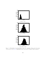
Hub-height velocity histograms for tuft video data sets . . . . . . . . . . . 100
5.3
Effect of dateset length on velocity fluctuation . . . . . . . . . . . . . . . . 101
5.4
Pitch mechanism activity during a grid disconnection . . . . . . . . . . . . 103
5.5
Change in pitching moment at different pitch angles . . . . . . . . . . . . . 104
xiv
5.6
Relation between pitch angle and rotor speed . . . . . . . . . . . . . . . . 105
5.7
Springs in pitch mechanism . . . . . . . . . . . . . . . . . . . . . . . . . . 106
5.8
Binned power curves for Wenvor 30 wind turbine . . . . . . . . . . . . . . 106
5.9
Power curve comparison before and after pitch adjustment . . . . . . . . . 108
5.10 Binned CP –λ curves for Wenvor 30 wind turbine . . . . . . . . . . . . . . . 109
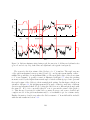
5.11 Blade stall during grid disconnection in high winds . . . . . . . . . . . . . 111
5.12 Sample extreme stall case demonstrating algorithm ability to locate tufts . 112
5.13 Sample image showing characteristic stall pattern on blade . . . . . . . . . 114
5.14 Binned ζ–U0 curves . . . . . . . . . . . . . . . . . . . . . . . . . . . . . . . 115
5.15 Comparing quality of tuft images from May 12 and November 1 . . . . . . 117
5.16 Azimuthal variation in stall fraction . . . . . . . . . . . . . . . . . . . . . . 118
A.1 Aligning the tuft layout template on the blade . . . . . . . . . . . . . . . . 137
A.2 Template to aid in layout of tufts on blade . . . . . . . . . . . . . . . . . . 138
A.3 String-pot calibration curve . . . . . . . . . . . . . . . . . . . . . . . . . . 139
A.4 Hub propeller anemometer test setup . . . . . . . . . . . . . . . . . . . . . 140
A.5 Propeller anemometer calibration curves . . . . . . . . . . . . . . . . . . . 141
A.6 Rotor speed sensor printed circuit board . . . . . . . . . . . . . . . . . . . 142
A.7 Rotor speed sensor circuit and pinout diagrams . . . . . . . . . . . . . . . 142
A.8 Mount for the yaw direction sensor . . . . . . . . . . . . . . . . . . . . . . 143
A.9 Instrumentation power supply from base to nacelle . . . . . . . . . . . . . 144
A.10 Yaw slip-ring . . . . . . . . . . . . . . . . . . . . . . . . . . . . . . . . . . 146
A.11 Close view of brushes on hub slip-ring . . . . . . . . . . . . . . . . . . . . . 147
A.12 Interior of hub slip-ring . . . . . . . . . . . . . . . . . . . . . . . . . . . . . 148
A.13 Hub slip-ring as installed on the turbine . . . . . . . . . . . . . . . . . . . 148
B.1 Screenshot of main data acquisition VI . . . . . . . . . . . . . . . . . . . . 151
B.2 Detailed network diagram . . . . . . . . . . . . . . . . . . . . . . . . . . . 152
D.1 First image from tuft demonstration video with algorithm steps labelled . . 159
D.2 First image frame from tuft demonstration video . . . . . . . . . . . . . . . 160
xv
List of Tables
2.1
Wind turbines in Eggleston and Starcher study compared alongside Wenvor
30 turbine . . . . . . . . . . . . . . . . . . . . . . . . . . . . . . . . . . . .
25
2.2
Details of NREL Phase II, IV, and VI wind turbines
. . . . . . . . . . . .
31
3.1
Details of the Wenvor 30 wind turbine . . . . . . . . . . . . . . . . . . . .
39
3.2
Met tower instrumentation from NRG Systems . . . . . . . . . . . . . . . .
52
3.3
Data acquisition units on wind turbine . . . . . . . . . . . . . . . . . . . .
56
3.4
Sampling frequencies for all sensors . . . . . . . . . . . . . . . . . . . . . .
59
5.1
Accuracy of determination of azimuthal position . . . . . . . . . . . . . . .
98
5.2
Tuft data statistics for each video data set . . . . . . . . . . . . . . . . . .
99
A.1 List of instrumentation and devices at the field test site . . . . . . . . . . . 136
B.1 DAQ unit specifications . . . . . . . . . . . . . . . . . . . . . . . . . . . . 149
B.2 Amount of cropping from each edge of video . . . . . . . . . . . . . . . . . 150
C.1 Sources of uncertainty in instrumentation. . . . . . . . . . . . . . . . . . . 155
xvi
Nomenclature
Roman Letters
A area swept by wind turbine rotor [m2 ]. 17
B span of a wing or wind turbine blade [m]. 11, 12
CD coefficient of drag [–]. 8, 9, 15, 34, 120
CL coefficient of lift [–]. 8, 9, 14, 23, 33, 109
CP coefficient of power [–]. 17, 18, 107, 109, 156
CP,max maximum coefficient of power [–]. 18, 107
D rotor diameter [m]. 13, 17, 45, 47, 49, 140
FD drag force on an airfoil [N/m] (or [N]). 7, 8
FL lift force on an airfoil [N/m] (or [N]). 7, 8
M aerodynamic pitching moment [N·m]. 15, 103
N blade flex position [–]. 65, 69, 72, 77, 78, 85, 87, 88, 112
Nj blade flex position from previous image [–]. 67, 72, 78
Ntot total number of blade flex positions [–]. 69, 84–89
P electrical or mechanical power output by turbine [W]. 16, 51, 102, 103, 106, 107,
110, 155
P0 turbine power output corrected for sea level air density [W]. 16
R rotor radius [m]. 13, 14, 26, 28, 37, 39, 42, 63, 113
xvii
R∗ specific gas constant for air (287 J/kg·K). 52
Re Reynolds number [–]. 8, 109
S planform area of airfoil, wing, or blade [m2 ]. 8
T0 ambient temperature [K] or [◦ C]. 13, 52, 95, 155
U wind speed [m/s]. 7, 8, 19
U0 upwind (hub height) velocity [m/s]. 13, 14, 18, 19, 95, 106, 107, 118
U20 velocity measured at 20 m [m/s]. 102, 103, 110, 155
Uref reference velocity in velocity profile extrapolation [m/s]. 19, 95
VRMS root mean squared velocity ratio [–]. 101
W relative velocity vector at blade section [m/s]. 13–15, 19, 103
a (sectional) axial induction factor [–]. 13, 14
a0 (sectional) tangential induction factor [–]. 14
c airfoil chord length [m]. 7, 8
e eccentricity of an ellipse [–]. 72
f electrical line frequency [Hz]. 50, 51
ht turbine height [m]. 13
hC camera offset from blade [m]. 25
n number of tufts located by the algorithm [–]. 72, 73, 76–78, 81–87, 90–92, 98, 112,
116, 156, 157
ns number of tufts tagged as stalled by the algorithm [–]. 76, 80, 83, 156, 157
nmin desired minimum number of tufts located by the algorithm [–]. 72, 73, 84–89
p0 atmospheric pressure [Pa]. 13, 52, 95, 155
r radial position along the blade or rotor [m]. 13, 14, 26, 63, 113
t time [s] (unless specified). 47, 90–92
z height above ground [m]. 19
xviii
z0 roughness height using logarithmic boundary layer approximation [m]. 19
zref reference height for velocity profile extrapolation [m]. 19, 95
Greek Letters
Ω rotational speed of the wind turbine rotor [rad/s] or [rpm]. 13, 18, 47, 50, 102–105,
107, 110, 155
Φ blade azimuthal angle: increases in direction of rotation (0◦ at top) [◦ ]. 13, 14, 19,
30, 95–97, 118–120
Ψ yaw offset with respect to wind direction (positive clockwise) [◦ ]. 13, 14, 19, 26, 29
Ψ0 orientation angle of turbine with respect to True North [◦ ]. 13, 47, 98, 99, 141, 155
α angle of attack of airfoil [◦ ]. 7, 8, 15, 30, 33, 103, 115
β wind shear exponent in power law approximation [–]. 19, 95, 119
δB angle of blade surface curvature at tuft anchor point [◦ ]. 75
δIP angle of tuft in image plane with respect to horizontal [◦ ]. 74–76, 79
δL lift angle of tuft off blade surface [◦ ]. 25, 75
δR angle of tuft radially with respect to chordwise direction [◦ ]. 25, 28, 31, 75, 76, 79
δtilt angle of camera tilt with respect to rotor plane [◦ ]. 25, 26, 75
λ tip speed ratio [–]. 17, 18, 28, 107, 108, 156
µ dynamic viscosity [kg/m·s]. 8
ρ density [kg/m3 ]. 8, 16, 52, 95, 156
ρ0 sea level air density (1.225 kg/m3 ). 16
φ angle of air velocity relative to turbine blade movement [◦ ]. 14
τ local twist angle of wind turbine blade [◦ ]. 14
θ pitch angle of wind turbine blade tip [◦ ]. 14, 102–105, 110, 111, 155
ζ fraction of blade stalled [–]. 73, 76–81, 83, 110, 112–118, 156, 157
ζmanual manually-estimated fraction of blade stalled [–]. 79, 80, 83
xix
Acronyms
BEM Blade Element Momentum. 14, 27, 119
CFD Computational Fluid Dynamics. 32
CNC computer numerical control. 145, 147
csv comma-separated value. 53, 59, 136
DAQ Data Acquisition. 54–57, 59, 60, 62, 149, 150, 154, 155
HD High Definition. 54, 63, 64, 117
IEC International Electrotechnical Commission. 16, 95, 105–107
mp4 MPEG-4. 53, 54, 57, 63, 64, 85, 88, 136
NASA National Aeronautics and Space Administration. 31
NI National Instruments. 56, 149
NREL National Renewable Energy Laboratory. 24, 30–34, 57, 109, 115, 119, 120
NRG NRG Systems. 36, 48, 52, 59, 136, 143, 155
NWTC National Wind Technology Center. 30
PCB Printed Circuit Board. 141, 142
PVC polyvinyl chloride. 145, 147
PWM Pulse Width Modulation. 47, 48, 136, 141
rms root mean squared. 101
RMY R.M. Young Company. 45, 48, 49, 59, 95, 98, 136, 143, 155
xx
RTK Real Time Kinetic. 35, 38
rpm rotations per minute. 18, 25, 28, 31, 37, 47, 50, 56, 96, 136, 140
SCADA Supervisory Control and Data Acquisition. 49
UAE Unsteady Aerodynamics Experiment. 30, 32, 34
VI Virtual Instrument. 59, 149, 151
xxi
Chapter 1
Introduction
1.1
Horizontal-axis wind turbines
The first recorded use of a wind-powered milling machine which could be rotated to face
the wind was in 1185 in Yorkshire [1]. Such windmills had four sails fixed to a rotating
horizontal axis and were used for tasks such as grinding wheat or for pumping water in
The Netherlands [2]. After that time, wind machines did not change considerably until
just over 100 years ago when they were introduced as a means of producing electricity. An
example of an old Dutch windmill is shown alongside a modern 2.3 MW wind turbine in
Figure 1.1.
Canada In Canada, the first commercial (grid-connected) wind turbines were installed
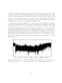
in Alberta in 1993 [3]. A summary of Canadian development activity is presented in Figure
1.2: the number of installed wind farm sites has increased to 174 at the time of writing.
Size For the purposes of the present work, a distinction will be made between smalland large-scale wind turbines. The definition used by Wood [4] will be used, whereby any
turbine with less than approximately 50 kW power output is considered small-scale. Any
turbine above 500 kW will be considered large-scale, with medium-scale lying between the
two. In addition, a micro-scale turbine is approximately 1 kW or less.
Components Figure 1.3 is a schematic of the components of a modern horizontal-axis
wind turbine. This example has a tail (as is typical of small-scale wind turbines) which
1
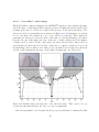
(a) Dutch windmill in Heerde, The Netherlands
(b) 2.3 MW turbine near Kingston, Canada
1600
8000
1400
7000
1200
6000
1000
5000
800
4000
600
3000
400
2000
200
1000
0
1990
1995
2000
2005
2010
Total Installed [MW] (−−)
Yearly Installed [MW/yr] (bars)
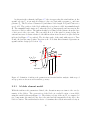
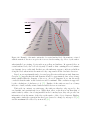
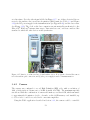
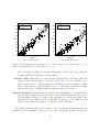
Figure 1.1: Horizontal axis wind machines. Photos by the author.
0
2015
Figure 1.2: The Canadian grid-connected wind industry started in 1993. Bars use left-hand scale;
line uses right-hand scale. Data from [3].
2
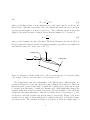
orients the wind turbine into the wind. The aerodynamic parts of the turbine—the blades—
are fixed to the hub at their roots; this all rotates as one component called the rotor. The
rotor turns the main shaft which is connected to a gearbox (unless the turbine is a direct
drive machine) to step up the rotational speed to an appropriate speed for the generator.
The main shaft, gearbox, and generator are housed within an enclosure called the nacelle.
This structure sits on top of the tower, completing the wind turbine. This example is
modelled after the Wenvor Technologies wind turbine introduced in Section 1.3 but is
typical for most small-scale turbines. For wind turbines with a blade length over 5 m long,
generally an active control replaces the tail [5].
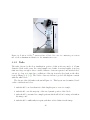
Rotor
Main Shaft
Gearbox
Generator
Hub
Tail
Blade root
Nacelle
Blade
Tower
Blade tip
Figure 1.3: Major components of a small-scale horizontal-axis wind turbine.
Design Wind turbines may have two different orientations called “upwind design” or
“downwind design.” If the rotor is directly in the path of the wind, it is “upwind” of the
tower. In contrast, if the wind encounters the tower before the rotor, this is a “downwind”
design. Upwind designs are currently standard; among other issues, the tower causes
a severe change in the blade aerodynamic loads each time a blade passes behind it in
downwind designs [6–9].
3
1.2
Motivation
In the 1950s, large centralised power generation stations in Denmark had the potential to
make the electrical grid unreliable, so a distributed network of wind turbines was proposed
[10]. A similar argument could be made for the present-day use of a collection of small-scale
wind turbines in communities not yet connected to the continental electrical grid. Often
the sole source of electricity generation in such remote communities is diesel generators, yet
the difficulty in accessing these locations leads to high maintenance and fuel transportation
costs.
In light of this, the research and development of small-scale wind turbines remains relevant, especially because scaling parameters exist to relate their performance to large-scale
turbines (see Section 2.2.3). Small-scale wind turbines are much easier and, in absolute
terms, cheaper to acquire, instrument, and maintain than large-scale machines. Yet on
a cost per energy basis, they remain more expensive than large-scale wind turbines and
hence merit further research.
Small-scale wind turbines often use a stall-regulated design (see Section 2.2.2) and are
thus guaranteed to encounter stall during their normal operation. Aerodynamic stall can
affect wind turbine noise [11] and fatigue life [12] due to unpredictable blade loads. One
established technique to study aerodynamic stall involves attaching short pieces of yarn
(“tufts”) to a blade and imaging their behaviour during operation (see Section 2.3). The
images or video are then manually reviewed in a “time-consuming” [13] process whereby
researchers look for small portions of the video when tuft patterns show strong trends. Such
subjective analysis may lead to exaggerated results and biased conclusions. In the present
day, however, the capture, storage, and processing of high quality images and video is
possible with a high degree of accuracy, speed, and volume. This has significantly increased
the feasibility of processing image data with computer code. The strong advantage of this
lies in the opportunity to collect and analyse long time periods of tuft flow visualisation
video yielding a much higher statistical significance to the results. This thesis presents the
development and application of a digital image processing algorithm to determine blade
aerodynamic performance on a small-scale wind turbine.
1.3
Project overview
The project timeline consisted of the five phases outlined below. Phases II–IV are the
subject of the present work.
4
Phase 0: Feasibility study In order to determine the feasibility of using wind energy
in the Waterloo region, a meteorological (met) tower was installed in 2008 at the UW
Wind Energy Group’s test site [14]. The feasibility study determined that while the wind
resource may not be economically viable, it is sufficient to permit installation of a wind
turbine for research purposes. The machine chosen was the Wenvor 30 wind turbine.
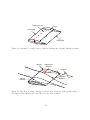
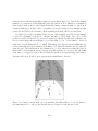
Phase I: Wind turbine installation The Wenvor 30 is a two-bladed horizontal-axis
wind turbine with an upwind design and rated power output of 30 kW. This wind turbine is
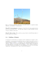
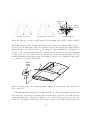
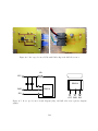
useful for research because it features guy wires and a winch system (shown in Figure 1.4)
to allow the turbine to be tilted down to the ground as shown in Figure 1.5. This feature
permits instrumentation and maintenance without the need for costly and time-consuming
lifting devices. The wind turbine was commissioned in the summer of 2012.
Main guy wire
Figure 1.4: The winch at left, operated by a hydraulic pump (not shown), enables the lowering
and raising of the wind turbine using the main guy wire after the others are removed.
Phase II: Instrumentation and data collection Installation of sensors measuring
various mechanical and operational characteristics of the turbine was completed in the
spring of 2013. Details of the instrumentation are provided in Chapter 3 and Appendix A.
The data acquisition (DAQ) system was configured to enable continuous data collection.
However, due to the combination of trouble-shooting required in the early months and very
low summer winds, several separate data campaigns were conducted throughout 2013.
5
Figure 1.5: The tilt-down function of the Wenvor wind turbine makes for comparatively simple
maintenance and installation of instrumentation.
Phase III: Code development Computer code was developed to time-synchronise data
from the various DAQ devices. The tuft image digital processing algorithm was then
developed, validated, and revised.
Phase IV: Data analysis The operation, power production, and stall characteristics of
the wind turbine were analysed.
1.4
Outline of thesis
A background on wind turbine aerodynamics and flow visualisation is essential to understanding the concepts presented in this thesis; these are included along with a review of
relevant literature in Chapter 2. A description of the experimental setup is the topic of
Chapter 3. Chapter 4 is devoted to the digital image processing algorithm. The results and
successful application of the method follow in Chapter 5. A more detailed description of
the design, calibration, and installation of the instrumentation, as well as the uncertainty
analysis and a demonstration video, may be found in the appendices.
6
Chapter 2
Background
In the first two sections of this chapter, a brief theory of aerodynamics will be outlined
for standard airfoils and wings and for wind turbines. Following that, the topic of tuft
flow visualisation will be explored. The final section is a review of the existing literature
regarding aerodynamics and flow visualisation of wind turbine blades. A more thorough
background on aerodynamics may be found in [15–18]; see [19–22] for a more complete
exploration of various types of flow visualisation including the tuft method.
2.1
2.1.1
Theory of aerodynamic lift and drag
Two-dimensional airfoils
When an object moves relative to a fluid it develops a pressure distribution on all its
surfaces. This pressure may be integrated to determine the resulting forces on the object.
On an airfoil, these forces are typically separated into lift and drag, which act perpendicular
to and parallel to the freestream velocity, respectively. The freestream velocity, or bulk
movement of the airfoil relative to the fluid, is represented by U in Figure 2.1. The angle
between the chord c—the linear distance between the leading edge and trailing edge—and
the freestream velocity is called the angle of attack, α. Also labelled in the figure are the
lift and drag forces FL and FD which pass through the aerodynamic centre of the airfoil.
The lift and drag forces are calculated as follows [23]:
1
FL = CL ρU 2 S
2
7
(2.1)
and
1
(2.2)
FD = CD ρU 2 S
2
where ρ is the fluid density, S is the planform area of the airfoil, and CL and CD are the
lift and drag coefficients, respectively. On a two-dimensional airfoil, the forces and span
are given per unit length, so S may be replaced by c. The coefficients depend on the profile
(shape) of the airfoil, its angle of attack, and its Reynolds number Re [24] given by:
Re =
ρU c
µ
(2.3)
where µ is the dynamic viscosity of the fluid. The Reynolds number also has an effect on
the flow separation (discussed in the following paragraphs), especially in very small-scale
wind turbines where it is on the order of 105 [25].
Leading edge
U
FL
α
FD
Trailing edge
c
Figure 2.1: Schematic of an airfoil with chord c. The freestream wind speed U meets the leading
edge at angle of attack α and causes lift force FL and drag force FD .
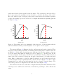
The general shape and order-of-magnitude of the lift and drag coefficient curves are
presented in Figure 2.2. On both curves, the point of highest CL is indicated. This is an
important point, because at this angle of attack, the boundary layer on the airfoil begins
to separate from the surface, causing aerodynamic stall. Stall significantly changes the
pressure distribution around the airfoil. On average, the bottom surface of the airfoil has
a higher pressure than atmospheric, while the top surface has a lower pressure [23]; they
are therefore called the pressure and suction surfaces, respectively. Figure 2.3(a) shows
an airfoil at low angle of attack with the flow completely attached on both the pressure
and suction sides. The schematic in Figure 2.3(b) shows an airfoil at a higher angle of
8
attack where the flow has separated from the surface. The separation point is labelled at
the location where the streamlines of the flow fail to conform to the shape of the airfoil.
Here, the “stalled region” is the part of the airfoil on the suction side from the separation
point to the trailing edge and is evidenced by a highly turbulent wake (swirling patterns
in Figure 2.3(b)).
max CL
1.0
1.0
0.8
0.8
CL [-]
CL [-]
max CL
0.6
0.6
0.4
0.4
0.2
0.2
0
5
10
α [°]
15
0
(a) lift curve
0.01
0.02
CD [-]
0.03
(b) drag polar
Figure 2.2: Typical shape and order-of-magnitude of lift-drag curves. CL increases almost linearly
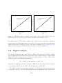
until its maximum at which point the magnitude of CD begins to increase rapidly.
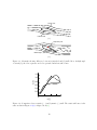
The images in Figure 2.3 illustrate the flow conditions at fixed angles of attack. When
the angle of attack changes with time, the stalling characteristics may be different as shown
in Figure 2.4. As the angle of attack increases with time, the CL may continue to increase
above the static value until the stalling process is complete [8]. At this point, the lift
decreases abruptly. As the angle of attack decreases with time, it takes a finite amount of
time for the flow to reattach; by this point, the angle of attack may be below the static stall
value. Hence, a hysteresis loop develops, with CL values above and below those predicted
by static stall models and experiments. The solid line shown in Figure 2.4 is the so-called
dynamic stall loop, with arrows indicating the direction of angle of attack change. The
dotted line provided for comparison is the same curve as in Figure 2.2(a).
The behaviour of airfoils becomes more complex when they have finite dimensions. The
following section outlines the additional considerations pertaining to three-dimensional
wings.
9
Suction side
Pressure side
(a)
Separation point
“Stalled region”
(b)
Figure 2.3: Schematic showing difference between (a) attached and (b) stalled flow. At high angle
of attack (b), the flow separates and a low-pressure turbulent wake forms.
1.2
CL [-]
1.0
0.8
0.6
0.4
0.2
0
5
10
15
α [°]
Figure 2.4: Comparison between static (· · ·) and dynamic (—) stall. The static stall curve is the
same as that in Figure 2.2(a). Adapted from [8].
10
2.1.2
Three-dimensional wings
A three-dimensional wing is shown in Figure 2.5; the third dimension is called the span B.
Also shown here are the thickness and the quarter-chord line; the latter is the set of points
which are located on the chord line one quarter of the way from the leading edge to the
trailing edge.
Due to their finite span, wings encounter end effects. On wind turbine blades, the effect
is noticeable at the root and tip (see Figure 1.3), though the tip has a larger effect on the
lift [17]. Because of the different pressures on the two surfaces of the wing, a pressure
discontinuity would occur where they meet at the tip. Instead, as illustrated in Figure 2.6,
a vortex is formed as the air on the pressure surface is pushed around the tip to the suction
surface, causing a reduction in lift. The advantage of the flow deflection is a reduction in
the angle of attack which reduces the likelihood of stall [26]. Since stall causes a large
turbulent wake region and thus unpredictable loads, this is beneficial to the fatigue life of
the wing.
In summary, the lift generated by an airfoil is a function of its profile, angle of attack,
and Reynolds number. In particular, as the angle of attack is increased, the airfoil reaches
a critical point beyond which the boundary layer begins to separate from the airfoil and
a stalled region develops. On a wing, the angle of attack is reduced at the tip causing a
decrease in lift and a decrease in the likelihood of stall. As mentioned in the beginning
of this chapter, this is a basic introduction; there are other references available which
discuss this theory in more detail. The next section will expand on this discussion with an
exploration of the aerodynamics of wind turbines.
2.2
Aerodynamics of wind turbines
Wind turbine aerodynamics is derived from, but more complex than, the aerodynamics of
airfoils and wings. The main difference is that a wind turbine’s wings (henceforth called
“blades”—see Figure 1.3) are rotating. This means that the term “freestream velocity”
from Section 2.1 is inadequate to describe the motion of the air relative to the blade.
Instead, two new concepts are defined:
Upwind velocity: (also called the “wind”) the speed and direction of the air approaching
the wind turbine from sufficiently far away so as to not be affected by it.
Relative velocity: velocity of the air relative to the blade. This will be discussed in the
next section.
11
Quarter-chord line
Chord
Leading edge
B
Trailing edge
Thickness
Figure 2.5: Schematic of a wing: a series of airfoils extending into the third dimension, span B.
Wing tip
Outward flow
deflection
Tip vortex
Inward flow
deflection
No flow
deflection
Figure 2.6: Tip effect on a wing. The tip vortex is formed as the air on the pressure surface of
the wing moves around the tip to meet the air on the suction surface.
12
As shown in the schematic in Figure 2.7, the air approaches the wind turbine at the
upwind velocity U0 at an angle Ψ relative to the rotor axis with a pressure p0 and temperature T0 . The rotor has a diameter D (and thus a blade length of R) and rotates at a
speed of Ω. The position of the blade within the rotor plane is called its azimuthal angle
Φ. The azimuthal angle starts at 0◦ when the blade points upwards and increases in the
direction of blade rotation. The turbine height ht is defined as the distance from the base
of its tower to the rotor axis. The yaw angle Ψ is 0◦ if the wind is oriented along the
axis and increases clockwise relative to the turbine when viewed from above (the direction
indicated in Figure 2.7 is positive). The absolute angle of the wind with respect to True
North, Ψ0 , has the same positive direction as Ψ. Note that this schematic represents an
upwind turbine design (see Section 1.1).
Ω
Φ
Ψ0
D
North
U0,p0,T0,ρ
ht
Ψ
Rotor Plane
Figure 2.7: Definition of turbine-scale parameters used in wind turbine analysis. Airflow speed
and properties are shown as well as turbine geometry.
2.2.1
A blade element model
With the turbine-scale parameters defined, the discussion may now turn to the aerodynamics of the blades. The cross-section of the blade at a radial location r is modelled
using the variables shown in Figure 2.8. The relative velocity of the air, W , is comprised of
two components: the axial velocity due to the wind and the tangential velocity due to the
blade’s rotation. The axial induction factor a determines the reduction in axial velocity at
13
the rotor due to momentum exchange between the air and rotor; the tangential induction
factor a0 determines the amount by which the air begins to rotate in the wake of the turbine
in reaction to the opposing motion of the rotor [26]. The velocity triangle shown in the
figure with W at an angle of φ relative to the rotor plane results from the combination
of the induction factors, wind speed, rotor speed, and radial location. At the blade tip
where r = R, the angle of the chord with respect to the rotor plane is the pitch angle θ.
The local twist angle is τ . Pitch and twist are defined as positive in the direction which
orients the leading edge into the wind as in Figure 2.8. The combination of airfoil profiles,
twist, pitch, rotor speed, and rotor diameter provides sufficient information to model the
performance of a wind turbine at different upwind conditions. This is modelled and solved
iteratively using the Blade Element Momentum (BEM) method. For a derivation of BEM
theory and the parameters in Figure 2.8, see [26–28].
θ+τ
rΩ(1+a')
φ
α
Rotor plane
U0(1-a)
Chord line
W
Figure 2.8: Definition of geometry and velocity parameters at a blade element. Note this φ is
different from the blade azimuthal position Φ in Figure 2.7.
The angle of attack on the blade thus depends on the radial position, rotational speed,
wind speed, pitch, twist, and the profile (which partly governs the induction factors). In
addition, by varying the direction (not magnitude) of the wind speed vector U0 (1 − a) in
Figure 2.8, the angle of attack can be changed. This occurs during a yaw angle offset with
Ψ 6= 0: as the blade rotates, the angle of attack may change by a significant amount as a
function of the azimuthal angle Φ thereby putting parts of the blade into and out of stall
and causing large cyclic blade loads [12]. This is a highly undesirable state of operation:
as mentioned in Section 2.1.2, loads are difficult to predict during stall; such cyclic loads
also decrease the fatigue life of the blades.
The angle of attack may also be varied by changing the blade pitch during operation.
This is typically done to optimise power (see Section 2.2.2) and can be by one of two
methods: pitch-to-feather or pitch-to-stall. Pitch-to-feather, or feathering, increases the
pitch angle θ as defined in Figure 2.8 which reduces the angle of attack, and thereby
CL . Pitch-to-stall does the opposite: by increasing the pitch angle, the angle of attack
14
is increased beyond the stall point resulting in an increase in CD (see Figure 2.2(b)).
Feathering is generally preferred because the blade incurs more predictable forces than in
stalled flow [29].
Blade pitch may be controlled aerodynamically by accounting for the aerodynamic
pitching moment M [30] as shown in Figure 2.9. If the blade is allowed to pitch about a
point called the pitching centre, then the combination of aerodynamic pitching moment
and the lift and drag forces will create a total moment on the blade segment which acts
to pitch it in one direction. As discussed previously, the aerodynamic forces are strongly
dependent on the relative velocity W and the angle of attack α. This is therefore a passive
method for controlling blade pitch which does not require powered motors or actuators.
α
M
Direction of W
θ
Pitching centre
Figure 2.9: Definition of pitching moment at a blade element assuming no blade twist. This is
similar to Figure 1 in [30].
2.2.2
Wind turbine power output
The usefulness of a wind turbine is determined by its rate of conversion of the wind’s energy
into electrical power. In order to demonstrate this, a standard plot is shown in Figure 2.10
with the electrical power produced as a function of wind speed. The cut-in wind speed
is the speed at which the turbine begins to produce power. As the wind speed increases,
the power increases up to its maximum, or rated, power. Depending on the controls on
the wind turbine, the power curve may look different above its rated wind speed. This is
shown by the solid and dashed lines in Figure 2.10. With active controls, as in modern
medium- and large-scale turbines, pitching of the blades will result in a power curve with
a constant power output at and above the rated wind speed; the turbine is also shut down
15
for protection in extreme winds above its cut-out speed. This is represented by the solid
line in the figure.
Various methods exist to passively control the power at wind speeds above the rated
power. With passive pitch control [30], the power may be held fairly constant or increase
somewhat. With stall regulation, the power decreases as the blade becomes more fully
stalled and the lift is reduced [29]. As the wind speed is increased further into extreme
winds, the power in a stall-regulated turbine may surpass its rated power [31]. With a
“furling” design where the turbine is purposely oriented at a nonzero yaw angle above its
rated wind speed [32], the power may fall rapidly. All wind turbines, however, have a
cut-in wind speed and a rated power as well as some method of limiting the power in high
winds to protect them structurally, mechanically, and electrically.
P
Rated power
U0
Cut-in wind speed
Cut-out wind speed
Figure 2.10: Typical power curves for turbines with pitch control (—) and stall control (· · ·) (after
[29]). Note that without active controls, wind turbines will not shut down completely.
The manufacturer’s power curve for the 30 kW stall-regulated wind turbine used in
the present study is shown in Figure 2.11 [33]. The electrical power output is plotted on
the vertical axis against the wind speed. The International Electrotechnical Commission
(IEC) standard 61400-12 [34] specifies that the electrical power in such power curves is
normalised to sea level air density using the following equation:
P0 = P
ρ0
ρ
(2.4)
where P is the measured power output at the air density ρ and P0 is the corrected power
using sea level standard density ρ0 = 1.225 kg/m3 . This 10 m diameter turbine outputs a
maximum power of 34 kW at nearly 20 m/s. The high rated wind speed is unusual: it
16
is more typical for wind turbines to output their rated power at approximately 10 m/s–
12 m/s [35]. In order to compare this wind turbine with others of different scale and design,
therefore, a set of dimensionless parameters is needed.
50
P [kW]
40
30
20
10
0
0
5
10
15
20
25
U0 [m/s]
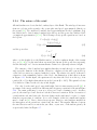
Figure 2.11: Manufacturer’s power curve for the Wenvor 30 turbine. 30 kW of power is output
at 17 m/s while the peak of 34 kW is output at 20 m/s. Adapted from [33].
2.2.3
Comparing wind turbine performance
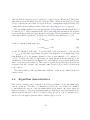
Two dimensionless parameters are essential to compare the performance of wind turbines:
the coefficient of power CP and the tip speed ratio λ. The CP is the ratio of power output
to the available power in the wind:
CP =
P
1
ρU03 A
2
(2.5)
where A is the area swept by the rotor, i.e. π4 D2 . According to linear one-dimensional
momentum theory, the maximum coefficient of power attainable is 0.593 [36]. For the
derivation, see, for example [26, 36]. This maximum CP is known as the LanchesterBetz-Joukowsky limit after the aerodynamicists who derived it in the early decades of the
twentieth century [37].
17
The second non-dimensional parameter is the tip speed ratio, λ, which is defined by
the following equation:
RΩ
(2.6)
λ=
U0
where Ω is in units of rad/s. The tip speed ratio is the ratio of the tangential velocity
of the blade tip to the (axial) upwind velocity. The CP –λ curve for the turbine used in
the present study is shown in Figure 2.12. This was calculated using the data from the
manufacturer’s power curve in Figure 2.11 and a rotor speed of 120 rotations per minute
(rpm) (see Section 3.2). Recalling that U0 is in the denominator of Equation 2.6, the wind
speed increases from right to left on this plot. The maximum coefficient of power, CP,max ,
is 0.33 at a tip speed ratio of 8.5 which represents a 7.5 m/s wind speed. This is a fairly
typical shape for a small wind turbine’s CP –λ curve [35]: the peak efficiency occurs at a
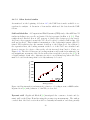
low wind speed less than the rated speed and is well below the Lanchester-Betz-Joukowsky
limit.
0.5
0.4
CP [−]
0.3
0.2
0.1
0
0
2
4
6
8
10
12
14
λ [−]
Figure 2.12: CP –λ curve for Wenvor 30 turbine using data from [33]. CP,max attained at λ = 8.5.
Before completing the present section on wind turbine aerodynamics, a discussion of
the nature of the wind is warranted.
18
2.2.4
The nature of the wind
All wind turbines are located in the boundary layer of the Earth. The wind speed increases
from zero velocity at the ground to the geostrophic wind speed approximately 1 km above
the ground [38]. Two standard boundary layer approximations are the logarithmic (log)
law, which can be derived using boundary layer theory, and the power law, which is based
on empirical approximation [38, 39]. The following velocity profile equations are based on
the log law:
U ∝ [log(z) + log(z0 )]
U (z) = Uref
log(z) + log(z0 )
log(zref ) + log(z0 )
(2.7)
and the power law:
U ∝ zβ
β
z
U (z) = Uref
zref
(2.8)
where z is the height above the Earth’s surface, z0 is the roughness height of the terrain
(see, ex. [38, 40]), β is the wind shear exponent (also known as the power law exponent),
and the subscript “ref” denotes measurements obtained at a (known) reference height.
The existence of the boundary layer implies that there is wind shear (i.e. a wind gradient) across the diameter of the turbine. Therefore, a higher velocity will occur at the top
of the blade’s rotation as compared with the bottom. The relative velocity W is therefore
a function of the azimuthal position of the blade. An illustration of this effect is shown
in Figure 2.13. In this figure, the upstream velocity when the blade is at the top of its
rotation (Φ = 0◦ ) is higher than when it is at the bottom (Φ = 180◦ ). The upwind velocity
U0 is therefore defined as the velocity at hub height.
Not only does the wind speed vary with height, but it is time-varying as well [41]. A
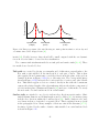
spectrum of the energy available in different wind frequency variations is shown in Figure
2.14. Two main peaks may be seen at a 4-day period and a 1-minute period. At these
periods, the wind speed and direction both show increased variation. From observation of
a wind turbine and wind vane, the direction change in the wind may be seen to be faster
than the response time of a turbine. A recorded example of this for a small wind turbine
may be found in [32]. Due to their slower response, therefore, wind turbines installed in
the atmosphere are in general not oriented into the wind. The angular difference between
the wind direction and rotor axis is the yaw offset, or yaw error, of the turbine given by Ψ
as previously defined in Figure 2.7.
19
U = Uref
ref
z
z = ht
β
( zz )
2 azimuthal
positions
U0
z=0m
Figure 2.13: Effect of wind shear on upwind velocity at a wind turbine. The power law is used
as an example velocity profile equation.
This concludes the brief discussion of the theory of aerodynamics of wind turbines.
These aerodynamic processes may be observed using the technique of tuft flow visualisation.
This is the subject of the following section.
2.3
Tuft flow visualisation
As an investigative technique, flow visualisation provides a qualitative picture of the motion of a fluid and its structures through primarily experimental means. When correctly
interpreted, reliable quantitative results can also be obtained. This section will focus on
the purposes and methods of tuft flow visualisation with an emphasis on its use for wind
turbines. A more in-depth discussion of specific studies will follow in Section 2.4.
2.3.1
Tuft methods
A tuft is a piece of fabric with one end held in place while the other is free to move in the
flow. Tufts are susceptible to forces such as gravity [42], centrifugal acceleration [43], and
20
Energy amplitude
Frequency
Synoptic peak
(4 days)
Diurnal peak
(24 hr)
Turbulent peak
(1 min)
Figure 2.14: Energy spectrum of the wind showing two main peaks in variation on four day and
one minute time scales. Adapted from [41].
inertia [44]. Ideally, however, these should all be small compared with the aerodynamic
forces in order for tufts to be used for flow visualisation.
Two common tuft attachment methods are tuft grids and surface tufts [20, 43]. These
two methods are described below:
Tuft grids are created by placing a rectangular grid of thin wires perpendicular to the
flow with a tuft attached at the intersection of each pair of wires. This is then
photographed from downstream to reveal flow directions in the plane of the grid; an
example is shown in Figure 2.15(a) for a delta wing test. The corresponding image
shown in Figure 2.15(b) indicates the location and size of vortices and other off-axis
flow. Tufts which appear as dots are oriented directly in line with the downstream
camera; the relative lengths of the other tufts may indicate the relative component of
velocity in that plane. Shimizu and Kamada [45] made use of this method to study
the near wake of a wind turbine model in a wind tunnel.
Surface tufts are attached to an object to indicate flow direction near its surface. Minitufts (0.04 mm diameter and 10 mm length as used by Mabey [46], for instance) may
indicate flow direction within the boundary layer [46]. Surface tufts are also used
as a binary indicator of attached or separated flow. This is explained in more detail
in the paragraphs below. Many examples of their use exist in the literature [47–51].
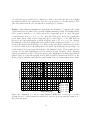
An image obtained by the author of surface tufts installed on a wind turbine blade
is shown in Figure 2.16.
21
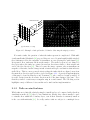
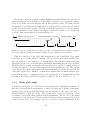
Main flow direction
Grid
De
lta
win
g
Tufts
Camera
(a) schematic of setup
(b) picture: republished from [52] with permission
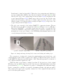
Figure 2.15: Example of tuft grid method behind a delta wing showing tip vortices.
For surface tufts, the question of what the tufts represent is complicated. With sufficiently small tufts (Merzkirch [42] proposed they not exceed 2 cm in length) in fully attached
flow, tufts may resolve the curvature of streamlines on a model wing in a wind tunnel [43].
In separated flow, tufts may lift from the surface. The stalled region is best defined by
the region where the tufts are oriented in random directions relative to their neighbours
and to the flow direction [43]. This is because the image captures only an instantaneous
snapshot of the tufts, but the change in tuft orientation in space and time is what indicates
stalled flow. This is a more general criterion than the tufts which are aligned away from
the main flow direction such as those circled in Figure 2.16. A practical implementation
of this may be found in Manolesos and Voutsinas [53] who considered a tuft as stalled “if
it would deviate from the chordwise direction most of the time during a [30 s] run.” Note
that they studied a stationary rectangular wing in a wind tunnel. The following section
highlights a major difference between this and a wind turbine implementation.
2.3.2
Tufts on wind turbines
While tufts are technically relatively simple to install and record compared with other flow
visualisation methods [54], they do have limitations. Firstly, they cannot usually be used
to visualise flow within the boundary layer, even if their diameter is extremely small as
is the case with mini-tufts [46]. Secondly, surface tufts are subject to centrifugal forces
22
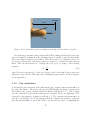
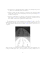
Tufts oriented away
from main flow direction
Main flow direction
Figure 2.16: Example of the surface tuft method on a wind turbine blade. Most tufts are oriented
with the main flow direction except for the few noted at the trailing edge. Photo by the author.
when installed on rotating objects such as propellers and turbines. In separated flow on
a wind turbine blade, the local velocity may be small so that centrifugal forces dominate
aerodynamic forces on the tuft. In that case, the tufts may appear to indicate radial flow
along the blade when in fact the main velocity component is in the chordwise direction.
Based on an experimental study of several propeller sizes with various tuft diameters,
Crowder [43] suggests that the tuft diameter should be approximately four orders of magnitude smaller than the diameter of the rotor. At rotor diameters above 4 m the study
concluded that the tufts’ radial deviation would be minimal. This conclusion is supported
by the calculations of Anderson et al. [55]. Further, if the tufts are used as a binary
indicator of stall, radially-oriented tufts in stalled flow are not an issue.
Tuft grids, in contrast, are stationary: the tufts are therefore only exposed to the
aerodynamic and gravitational forces. While their effect on the flow is less than that of
surface tufts by virtue of not being installed in the boundary layer, they also provide less
information about the nature of the flow on the surface of the object of interest. Further,
using surface tufts, the separation line has been observed to change by only up to 5% [47]
and the maximum CL reduced by at most 4% [43].
23
Based on the preceding discussion, surface tufts were deemed most appropriate for a
study of wind turbine stall in the outdoor environment. The following section will include
examples of such studies and others related to wind turbine blade stall.
2.4
Studies of wind turbine stall
This section focuses on studies of wind turbines in the literature regarding their stall
characteristics, design, and the features of tuft studies. There are a few noteworthy studies
which will be discussed in some depth: an outdoor study of three wind turbines using tuft
flow visualisation published in 1990 by Eggleston and Starcher [47]; a study of the stall on
a 1.2 m diameter turbine in a wind tunnel published in 2006 by Haans et al. [12]; and an
outdoor study of a 10 m diameter wind turbine using tufts and pressure measurements by
Maeda and Kawabuchi [50]. The section begins with brief mention of an early tuft study
[13] and concludes with a few studies using data from the National Renewable Energy
Laboratory (NREL) Unsteady Aerodynamics Experiment [56, 57].
2.4.1
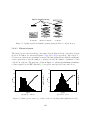
Pederson and Madsen tuft study
An early study by Pederson and Madsen [13] compared tuft video with a numerical simulation. The tufts were used to estimate the location of the separation line, though no
mention was made of the criteria used to do so and limited camera resolution prevented
viewing of the tufts near the tip. After recording one hour of video, only 8.5 s (five rotor
revolutions) were analysed in detail. A single revolution with a 0◦ yaw offset provided
the best agreement with the simulation. The authors described significant difficulty in
determining clear trends from the video and stated that manual interpretation of the video
“was rather time consuming” and that digital image processing “was discussed, but not
tested.” This is further evidenced by the fact that only 0.2% of the video (8.5 s out of one
hour) was actually analysed. They conclude that video evaluation techniques “must be
further developed.” This is one of the primary goals of the present work.
2.4.2
Eggleston and Starcher’s wind turbine comparison
In this early study [47], three downwind turbines were tested: the 6.3 m Enertech 21-5, the
9.9 m Carter 25, and the 13.5 m Enertech 44-50. Some of their specifications are listed in
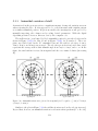
Table 2.1 along with the Wenvor 30 turbine used in the present study for comparison.
24
Table 2.1: Three wind turbines from Eggleston and Starcher [47] study compared alongside
Wenvor 30 turbine [33]. See also Table 3.1.
Enertech 21-5†
Rated power
5 kW
Design
downwind
Diameter
6.29 m
Blades
3
Rotor speed
105 rpm
Tip pitch
1.9◦
Blade twist
1.2◦
†
No longer in production.
Carter 25†
Enertech 44-50†
Wenvor 30
25 kW
downwind
9.91 m
2
120 rpm
0.0◦
33.8◦
50 kW
downwind
13.46 m
3
58 rpm
1.0◦
5.5◦
30 kW
upwind
10 m
2
120 rpm
3.0◦
0.0◦
Setup
In their study, the researchers recorded power output and the wind speed and direction
along with video of the flow visualisation. In order to achieve time synchronisation between
wind and flow visualisation, an anemometer was located on the turbine towers and a wind
shear exponent was used to estimate the hub-height wind speed from that.
Since all three turbines were of a downwind design, it was possible to mount the camera
on a boom projecting downwind perpendicular to the rotor plane to provide a more direct
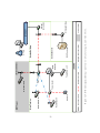
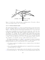
viewing angle. This is explained in Figure 2.17, where the camera is mounted on the boom
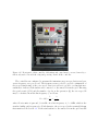
of length hC at an angle of δtilt towards the blade. A low resolution 35 mm film camera
recorded at 30 Hz and a sufficiently long exposure time was used so that tufts blurred when
“vibrating rapidly.” This blurring was used as a possible indication of stalled flow.
The ability of the tufts to follow the flow direction was estimated using the centrifugal
and the aerodynamic forces on the 2 mm diameter tufts. The authors expected a radial
deflection due to centrifugal forces on the order of (referring to Figure 2.17) δR = 2◦ .
This confirms the discussion in Section 2.3.2 suggesting that tufts are minimally affected
by centrifugal forces in attached flow. Thus, separated flow regions were assumed to be
indicated by radially-oriented tufts as well as those which were lifted from the surface
(δL > 0), oriented significantly away from the flow direction (δR 0◦ ), or significantly
blurred. Other than these general criteria, the authors do not give any indication of what
tuft angles or how much blurring are considered significant.
25
Tuft
δL
Camera
δR
Profile
C h o rd
hC
δtilt
Figure 2.17: Position of a tuft and camera relative to blade. Note the camera is tilted by δtilt
about the horizontal axis of its image plane.
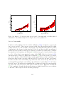
Results
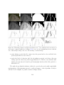
Approximately ten minutes of video were collected on each wind turbine. Full stall was
observed on the inboard section of both the Enertech machines even in low winds. In the
smaller 21-5, as much as 60% of the blade was stalled in 6 m/s–7 m/s winds, though there
was a strong tower effect due to the downwind design with the flow reattaching after the
tower passage. In the larger 44-50, some tufts near the trailing edge revealed stalled flow
at a radial location of r = 0.9R at 8 m/s; moving inboard from there, the separation line
moved towards the leading edge. This pattern, shown in Figure 2.18, was seen on both
Enertech turbines and was characterised as a “roughly triangular in shape” attached flow
region.
In contrast to this separation pattern, the highly twisted Carter 25 blade revealed
separation which began around midspan and spread quickly to the root and more slowly
towards the tip as wind speeds increased. The flow was completely attached up to wind
speeds of 7 m/s–8 m/s. This behaviour is more desirable than the stall which was present
at all wind speeds on the Enertech blades and provides a possible avenue for performance
improvement of untwisted wind turbine blades.
Additional notes
In more than one of the tests in their study, a nonzero yaw offset angle was observed. During
the 800 s (13.5 min) of video recording for the Carter 25 blade, an average yaw offset of
approximately 10◦ was observed. As mentioned in Section 2.2.1, a yaw offset Ψ can cause
dynamic stall and unpredictable cyclic loads on the blade. It also creates difficulty when
26
Triangular region of
attached flow
Blade
i
Blade ro
tip
s at
line eeds
n
o
i
d sp
a ra t
Sep ing win
s
a
ncre
Region of
separated flow
ot
Figure 2.18: Triangle-shaped region of attached flow on Enertech blades derived from [47]. As
winds increase, separation begins at inboard trailing edge and moves towards leading edge of tip.
interpreting tuft video: while reviewing a short time period of video, it may be difficult
to separate yaw offset effects from other effects such as wind speed and wind shear. This
suggests that a long sampling time is required for outdoor studies in order for long-timeperiod fluctuations to be smoothed by averaging. The researchers also noted that the sun
caused lost data every time it was in the camera frame. They suggest nighttime recording
may allow more control of lighting conditions. Again, a longer sampling time may mitigate
this effect by amplifying the sun’s movement and changes in the wind direction thereby
reducing the percentage of time in which the sun is in the image.
Overall, their study provides a baseline for outdoor flow visualisation studies of smallscale wind turbines. Many of the methods used therein were adapted for the present study.
However, the low camera resolution at the blade tip, yaw offset angle due to short data
set, and insufficiently-defined tuft stall angles suggest there is room for improvement. As
well, other studies have had conflicting interpretations on the meaning of different tuft
orientations. One such study is discussed in the next section.
2.4.3
Haans et al. micro-scale turbine study
A study by Haans et al. [12] compared both tuft visualisation and hot-film anemometry to
a BEM model prediction of stall on the blade of a 1.2 m diameter two-bladed micro-scale
wind turbine. The blades had a 2◦ pitch and 4◦ twist. The experimenters used an open-jet
wind tunnel with the turbine positioned at a 45◦ yaw angle 1 m downwind of the jet exit.
27
Setup
In contrast with the previous study by Eggleston and Starcher [47], a camera was positioned
downwind of the turbine and a strobe light was synchronised with the blade passage so
that the blade appeared to be stationary (actual rotor speed was 700 rpm). This is an
interesting choice of setup because by imaging the blade only once per revolution, all
transient information is lost. The authors reasoned, therefore, that radially-oriented tufts
indicated flow separation, whereas any tufts which were at an angle between chordwise and
radial indicated attached flow. Indeed, the images presented in the paper show tufts which
appear to be oriented either at δR = 30◦ or δR = 90◦ (i.e. radially—recall Figure 2.17).
This may have little applicability to larger wind turbines: the low Reynolds number on
the order of 105 is typical for micro-scale turbines [25], as is the high rotation rate which
causes high centrifugal loads. In spite of that, however, this simple criterion may be useful
as a starting point in the case of tuft images uncorrelated in time.
In addition to the tuft visualisation, hot-film anemometry measurements were made
immediately downwind of the wind turbine in azimuthal increments of 15◦ and radial
increments of 0.1R. The measurements were made to estimate the fluctuations of velocity
in the wake of the blade and thereby determine whether there was stalled flow. The extent
of the separated region was thus determined on the blade without the tufts installed.
Results
The hot-film measurements were compared with the observations of the tuft images and
yielded general agreement though there was an underprediction of the amount of stall by
the tuft method. A polar plot of the separated flow region around the azimuth at 8 m/s
(λ = 5.5) is shown in Figure 2.19 which contains part of Figure 12 in their work [12]. The
radial extent of stall ranges from 0.4R to 0.6R or 0.7R depending on the method used.
This mid-span stalled region in 8 m/s wind is similar to the Carter 25 blade in Eggleston
and Starcher’s study [47] discussed in the previous section. Due to the yaw offset, however,
only the azimuthal angles 330◦ –120◦ show evidence of stall. At this yaw offset angle, the
highest angle of attack is at the top (0◦ azimuth); yet the majority of azimuthal positions
with stall occur after that point in the blade’s rotation. This is suggested as evidence for
dynamic stall.
The authors suggest that a possible reason for the difference between the tuft and hotfilm methods may be that the criterion for determining which tufts were stalled was “too
stringent.” In other words, it is possible that tufts which are oriented at a radial angle of
less than δR = 90◦ represent stalled flow.
28
Figure 2.19: Stall extent in Ψ = +45◦ yaw offset (wind from left and into page). Bold dashed
line corresponds to the blade tip. Reprinted from [12] with author’s permission.
Their paper demonstrates that it is possible to interpret the general pattern of stall on
a blade from tuft images which are uncorrelated in time. The following paper confirms
these 45◦ yaw offset results on a 10 m upwind turbine.
2.4.4
Maeda and Kawabuchi study
In a paper by Maeda and Kawabuchi [50], the results of an outdoor study of a 10 m diameter
upwind turbine are presented. Surface pressures were measured with pressure taps and
dynamic pressures were measured with 5-hole pitot probes protruding upstream of the
leading edge of the blade. Aerodynamic forces were derived from the surface pressures and
inflow angles were calculated using the probe data. Tufts and a camera were also installed
to clarify interpretation of the data. 2.5 mm diameter yarn tufts which had lengths equal
to 15% of the chord at each location were spaced 10 cm (0.02R) apart in the spanwise
direction.
Results were presented for yaw offset angles of 0◦ and ±45◦ (a yaw drive controlled the
turbine’s orientation). With no yaw offset angle, an azimuthal variation in angle of attack
29
was seen as expected in wind shear (see Section 2.2.4) with the lowest α at an azimuth of
Φ = 180◦ and the highest at Φ = 0◦ . As in the study by Haans et al. [12] above, in a 45◦
yaw offset, most stalled tufts were observed at azimuth angles of 0◦ –90◦ . The off-axis wind
component was in the same direction as the blade’s movement at the top of its rotation,
again showing evidence for dynamic stall.
In personal correspondence with principal author T. Maeda [58], the subject of the
intrusion of the sun was brought up: given their combination of prevailing wind direction
and sun location, the researchers were mostly able to record video only in the afternoons.
This—and the weather in general—is a limitation of conducting flow visualisation experiments outdoors. Experimenters would therefore greatly benefit from the ability to record
and analyse flow visualisation data over longer time periods in order to minimise the percentage of weather-induced lost data.
A review of experimental wind turbine studies would not be complete without mention
of the NREL Unsteady Aerodynamics Experiment [56, 57]. This experiment, and several
studies which make use of its data, is the subject of the next and final section of this
chapter.
2.4.5
The NREL experiments
The NREL studies encompass both outdoor (Phases II–IV [56]) and wind tunnel (Phase
VI [57]) studies of a 10 m diameter wind turbine. The so-called Unsteady Aerodynamics
Experiment (UAE) took place over the years 1987 to 2000 and the data are still used as a
comparison for experimental and numerical studies today. The discussion of several such
studies follows, beginning with the UAE itself.
2.4.5.1
The Unsteady Aerodynamics Experiment
Tests The outdoor tests were conducted on a three-bladed downwind turbine at the
National Wind Technology Center (NWTC) outside Golden, Colorado in the United States
[56]. The Phase II and Phase IV wind turbine specifications are outlined in the first two
columns of Table 2.2. Two cameras were used for flow visualisation: one on a 3 m boom
extending downwind of the hub and the second fixed to the instrumented blade near the
hub. As with the studies discussed in Section 2.4.4, pressure measurements were made to
determine forces and angles of attack on the blade. 45 mm long 0.25 mm diameter (cited in
[56]—though based on their images, this may in fact be 2.5 mm) tufts were spaced 50.8 mm
apart in the chordwise and spanwise directions and fixed with quick-drying glue. Due to
30
glare during the day, many of the tests were completed at night. As such, twelve 100 W
lights were mounted on the camera boom to illuminate the blade. The signals were passed
through slip-rings and a single synchronising box was used to record the timestamp on all
data including the video. The data campaigns lasted only five or ten minutes, providing yet
another example of a short-duration outdoor tuft study and the accompanying difficulties
with interpretation. After the outdoor experiment, the turbine was heavily modified for
the wind tunnel experiment [57]: a yaw drive was added; the hub was converted to a
two-blade design; twisted tapered blades were used instead of the previous untwisted ones;
and the blades and nacelle orientation could be reversed so the turbine could operate in
a downwind or upwind configuration. Details of the wind turbine used in these Phase VI
studies may be found in Table 2.2. In all, 30 test sequences were completed in the 24.4 m by
36.6 m test section at the National Aeronautics and Space Administration (NASA) Ames
Research Center wind tunnel in its open-loop configuration.
Table 2.2: Details of NREL wind turbines from the Unsteady Aerodynamics Experiment Phases
II, IV, and VI.
Phase II [56]
Rated power 20 kW
Design
downwind
Diameter
10 m
Blades
3
Rotor speed 72 rpm
Tip pitch
12◦
Blade twist
0◦
Hub height
17.0 m
Chord
0.457 m
Study type
outdoor
Phase IV [56]
Phase VI [57]
20 kW
downwind
10 m
3
72 rpm
−9◦ to 12◦
45◦
17.0 m
0.457 m
outdoor
20 kW
upwind or downwind
10 m
2
72 rpm
fully adjustable (0◦ to 6◦ typically)
22.5◦
12.2 m
0.737 m–0.356 m
wind tunnel
Results As with the low-twist blades in the Eggleston and Starcher [47] study (see
Section 2.4.2), the researchers saw stall progress from the inboard to the outboard sections
of the untwisted blade used in the outdoor study [59]. Data from pressure distributions
and tuft images suggest that tufts may orient themselves in directions other than radially
even in fully stalled flow. This recurring theme in tuft visualisation studies suggests that
the threshold tuft angle above which a tuft may be considered to be in stalled flow lies
somewhere between δR = 0◦ and δR = 90◦ (see Figure 2.17). The exact angle, however,
may depend on the tuft geometry and camera setup.
31
simulation of wind turbine aerodynamics
2.4.5.2
M.-C. Hsu, I. Akkerman and Y. Bazilevs
Other derived studies
As mentioned at the beginning of Section 2.4.5, the UAE data is made available to researchers for analysis. A discussion of four studies which used the data from the UAE
follows.
Root flap bending moment (N m)
Stall and blade flex A Computational Fluid Dynamics (CFD) study of the full Phase VI
turbine including tower, nacelle, and twisted blades is presented in Hsu et al. [60]. Their
results showed attached flow at 80% span up to 10 m/s (the design speed was 8 m/s).
At 15 m/s, flow separated around the 50% chord location; by 20 m/s, full leading edge
stall was predicted. This is further demonstration of the design improvement offered by
twisted blades which reduce the amount of stall up to the design speed. In addition to
the separation lines, the bending moment at the root of the blade was calculated and
shown to increase by a factor of five as the velocity increased from 5 m/s to 25 m/s; see
Figure 2.20. The five-fold increase in bending moment would result in an unknown, but
not insignificant, movement of the blades as they flex toward the tower (see also [61]). In
Figure
Pressure
contours at
all cases.
a 5.digital
analysis
of80%
tuftspanwise
video,station
this for
may
give rise to an additional step where the blade
must be located in the image first before any tufts may be located.
NREL Exp.
ALE VMS
5
10
15
20
Wind speed (m/s)
25
30
6000
5000
4000
3000
2000
1000
0
NREL Exp.
ALE VMS
0
5
10
15
20
25
30
Wind speed (m/s)
(a)
(b)
Figure 2.20: Experimental (O) and numerical (◦) data for root bending moment on NREL turbine.
Reprinted from [60] with permission of John Wiley & Sons, Ltd.
he low-speed shaft (aerodynamic) torque and (b) the root flap bending moment for all cases. The simulation results are
pared with the NREL experimental data. The vertical bar represents plus and minus one standard deviation.
Dynamic stall Slepski and Kirchoff [62] investigated the occurrence of static and dystall on
theandPhase
II bending
turbinemoment
usingare
the
pressure
tap
measurements.
The authors
ged low-speed shaft namic
(aerodynamic)
torque
root flap
shown
in Figure
6 for
all wind
conclude
that “thedata
blade
section
flow well.
fieldAlthough,
is constantly
transition”
ll, the simulation results
and experimental
match
remarkably
there isin
a slight
under- and that generally
he aerodynamic torque for the high wind speed cases, and a slight over-predictions of the root flap bending
e low wind speed cases.
32
nd 8 show the normal and tangential force coefficients, respectively, at five spanwise stations for the wind
ered. The force coefficient is an integration of pressure limited to a spanwise station of the blade. Good agreeerimental data is generally found. The computed force coefficients mostly fall within one standard deviation
mental data. Exceptions are found for 10 and 15 m/s wind speeds at some spanwise stations.
peed shaft torque, root flap bending moment, and force coefficients represent the integrated effect of the
loads acting on the rotor blades. It is also of interest to assess the local flow behavior by examining a dise pressure coefficient over the blade surface. The sectional pressure coefficient Cp is computed using the
Root section
0.3
8
0.25
0.2
6
Cp [-]
Power [kW]
0.35
10
0.15
Axis of rotation
4
0.1
2
0.05
0
0
5 6 7 8 9 10 11 12 13 14 15 16 17 18 19 20 21 22 23 24 25
Wind Speed [m/s]
Tip section
Fig. 10. Performance comparison between twisted and non-twisted WT blades.
one of the two types of stall can be considered to exist on the blade inboard section during
any single revolution. In contrast, the outboard section is seen to be mostly attached. The
data were taken from 94 rotor revolutions at a wind speed of 14 m/s.
10
Fig. 7. Non-twisted wind turbine blade (Root section: R ¼ 1.258 m; tip section:
R ¼ 5.03 m).
Percent Power loss
Chord [m]
Pitch [deg]
Design Using numerical simulations, Lanzafame and Messina [63] compared the design
of the twisted tapered Phase VI rotor with a similar5 untwisted design. The highly twisted
Not twisted PHASE VI
◦
point at the design
wind speed of 8 m/s: the angle
10blade operated near the α = 8 stall 0.8
0
◦ pitch
◦
of attack ranged from α = 4 to α =0.712 along the blade span. Below the design wind
9
chord
-5
speed, there was no stall; at the design
wind speed,
stall began to occur. Full stall was
0.6
8
◦
◦
-10 span of 13 < α < 29 . In contrast,
predicted at 15 m/s with angles of attack
along the
0.5
7
the untwisted blade was significantly 0.4
more stalled -15
at the design speed with 3◦ < α < 28◦
6shown as the shaded region in Figure 2.21. Even at 5 m/s the angle of attack was predicted
0.3
◦
-20
At
all
of α24
4
6
8 wind
10
12speeds,
14
16the
18 range
20
22
5to reach 14 which is above the stall point for the airfoil.
0.2
for
the
twisted
blade
was
much
lower
than
for
the
untwisted
blade.
These
results
provide
Wind velocity [m/s]
4
0.1
evidence for the stall distributions seen in works
previously
discussed
when comparing
Fig. 11. Power loss at variable wind velocity (comparison between original
3
0
modified
WT
blades).
twisted
blades.
0
1 and untwisted
2
3
4
5They 6also may provide justification for using appropriately
Radius
[m]
twisted blades to
reduce
the amount of blade stall. As will be discussed in Section 3.2, the
Fig. 8. Chord
distribution
and constant
pitch for the non-twisted
wind turbine blade.
Wenvor
blade
is untwisted
and therefore
may benefit from a re-design with non-zero twist.
S809
1.5
1.3
1.1
Lift Coefficient [-]
0.9
0.7
0.5
0.3
0.1
-0.1 0
-25 -20 -15 -10 -5
5
10 15 20 25 30 35 40 45 50 55 60 65 70 75 80 85 90 95 100
-0.3
CSU; Re = 300,000
-0.5
CSU; Re = 500,000
-0.7
CSU; Re = 650,000
-0.9
OSU; Re = 750,000
OSU; Re = 1,000,000
-1.1
Angle of attack [deg]
DUT; Re = 1,000,000
Fig. 9. Lift coefficient along the non-twisted blade. Wind speed ¼ 8.0 m/s, pitch ¼ 3 (3 <a < 28 ).
Figure 2.21: Simulation of α and CL along untwisted NREL blade at wind speed of 8 m/s
(reprinted from [63] with permission from Elsevier). Shaded region represents the variation of α
along the blade span.
33
and
Azimuthal effect More recently, Sant et al. [64] investigated the difference in angles
of attack and aerodynamic forces around the azimuth for the Phase VI rotor in yawed
flow. Their results demonstrate a significant increase in normal force coefficients and
drag coefficients at the top of the blade’s revolution as the wind speed is increased above
the design speed. Below the design wind speed, however, at 5 m/s, CD does not vary
significantly with respect to the azimuthal position and all radial positions remain in the
attached regime (CD < 0.02). It is worth noting that even at 15 m/s where the blade is
fully stalled at the top of its rotation (CD as high as 1.7), all radial locations appear to
almost completely reattach at the bottom of its rotation (CD < 0.1) even though the angle
of attack at this range is predicted to be as high as 40◦ .
Far from being an exhaustive review of the NREL UAE, the studies discussed in the
preceding paragraphs give an indication of some of the flow features which may be expected
in the study of the untwisted blades on the Wenvor 30 stall-regulated upwind turbine.
Chapter 4 will draw on the studies discussed in this section in order to build the case
for the novel digital tuft image processing algorithm developed in the present study. First,
however, a description of the field test site is given in the next chapter.
34
Chapter 3
Experimental Setup
This chapter contains the details of the first phase of this work (Phase II of the project):
the installation of experimental equipment and collection of data. A brief description of
the test site and wind turbine are first provided in Sections 3.1 and 3.2 as background
related to the project Phases 0 and I. Following that, significant space is devoted to the
instrumentation in Section 3.3 and to the data logging in Section 3.4.
3.1
Overview of the test site
The wind turbine field test site is located just inside the boundary of the City of Waterloo
(site coordinates: 43.5◦ N, 80.5◦ W, 400 m elevation). Precipitation in the area can take the
form of rain, snow, or freezing rain, and temperatures reach as low as −30◦ C in the winter
months [65]. This caused design issues for the instrumentation which will be discussed
further in Section 3.3.
The site layout shown in Figure 3.1 includes the following: the Wenvor wind turbine;
a 50 m meteorological (met) tower almost directly south 100 m; a control centre including
the grid interconnection point located 137 m to the NW; and a wireless internet access
point situated 185 m to the SW. These locational measurements were made on December
14, 2012 with a Sokkia GRX1 GPS unit which has Real Time Kinetic (RTK) compensation
and was accurate to well under a metre (order of a few centimetres). A view of the wind
turbine and met tower from near the control centre is shown in Figure 3.2.
The wind turbine is situated on a small hill beside a bank of trees to the NE. The wind
rose is highly biased towards the NW, so the trees have little effect on the wind profile the
35
100
Control centre
N
↑
Metres North of Turbine
50
Turbine
0
Prevailing winds
−50
−100
Met tower
−150
Internet connection antenna
−200
−150
(a) imagery from [66]
−100
−50
0
Metres East of Turbine
50
(b) schematic view
Figure 3.1: Plan view of test site with distances acquired using a Sokkia GRX1 GPS unit.
majority of the time [14]. The turbine hub height is 31 m, which corresponds to a height of
36 m relative to the met tower. This is demonstrated in the profile view of the site in Figure
3.3. The profile shown is the vertical plane which includes the met tower and turbine; note
that the met tower is not in the direction of the prevailing winds. The instrumentation
on the met tower was primarily NRG Systems (NRG) components, as will be outlined in
Section 3.3. The instruments on the two towers in Figure 3.3 will be discussed further in
Sections 3.3.7 and 3.3.9.
36
Figure 3.2: Wind turbine (left) and met tower (right) viewed from 30 m NE of control centre.
3.2
The wind turbine
The wind turbine used in this study was a 10 m diameter 30 kW upwind horizontal-axis
machine designed and manufactured by Wenvor Technologies, Inc., a company local to the
region [67]. It has two 5 m long blades and rotates at a fixed nominal speed of 120 rpm.
The blades have a nominal 3◦ pitch and no twist. The turbine is a stall-regulated design
with a hub height of 31 m. Details of the geometrical and mechanical parameters are given
in Table 3.1. The exact airfoil is not known; however, the chord distribution and a typical
profile (at 0.49R) are shown in Figure 3.4.
Although the pitch in Table 3.1 is listed as 3◦ , this turbine is equipped with a passive
pitch mechanism which pitches the blades to feather at low rotational speeds and to stall
at high rotational speeds. The result is that the rotor continues to turn slowly in low
winds helping components and grease stay warmer in cold weather. As winds increase
to the cut-in speed, the blades assume their standard nominal pitch of 3◦ . The pitching
mechanism will be described in further detail in Section 5.2.1.
As mentioned in Chapter 1, the tower for this wind turbine has guy wires and a winch.
With these, the turbine may be lowered to the ground for instrumentation and maintenance. The turbine is supported laterally by four sets of guy wires, each consisting of four
cables at increasing heights. In the present installation, they are oriented approximately
towards the four intermediate directions (NW, NE, SE, and SW) and the main (topmost)
37
Vertical Distance [m]
50
50 m
40
40 m
36.3 m (as measured on met tower)
30
30 m
RMY Prop
20
20 m
NRG Cup
10
Met Tower
Turbine
0
Hill
−10
0
20
40
60
80
Horizontal Distance [m]
100
120
Figure 3.3: Profile view of field test site to scale looking due east. Instruments are described in
Section 3.3. Measurements made using a Sokkia GRX1 RTK GPS unit.
guy wire on the northwest guy anchor is attached to a winch. The winch and lowering
procedure were shown previously in Figures 1.4 and 1.5. An internal report [68] contains
a detailed description of the procedure.
A close-up view of the main components of the wind turbine is shown in Figure 3.5.
The tubular bars indicated are part of the centrifugal governor of the pitch mechanism.
A cut-away view of the components inside the wind turbine nacelle and hub are shown,
respectively, in Figures 3.6(a) and 3.6(b). Many of the components labelled here were
referred to in the schematic in Figure 1.3. There are a few differences: the main nacelle
casting and the hub casting are rigid cast parts to which the remaining components are
attached; and the spring enclosure contains two linear springs which counteract the centrifugal forces of the governor bars shown in Figure 3.5. The operation of these springs
will be discussed further in Section 5.2.1. The pictures in Figure 3.6 were taken of the
demonstration turbine at the Wenvor Technologies, Inc. manufacturing centre; the turbine
installed for this project was identical before instrumentation was installed.
38
Table 3.1: Details of the Wenvor 30 wind turbine.
Power
Diameter
Design
Blades
Tip pitch
Rotor speed
Blade twist
Taper
Hub height
Airfoil
Other
30 kW at 20 m/s
10 m
upwind with passive yaw
2
3◦
120 rpm
0◦
elliptical—see Figure 3.4(a)
31 m
see Figure 3.4(b)
gin pole & winch to lower for service and instrumentation
500
c [mm]
400
300
200
100
0
h
!
"2 i0.5
c = 4302 − 320000 Rr − 0.27
mm
0
0.2
0.4
0.6
0.8
1
r/R
(a) chord distribution and best-fit ellipse
y/c
0.1
0
−0.1
0
0.1
0.2
0.3
0.4
0.5
x/c
0.6
0.7
0.8
0.9
1
(b) blade profile at 0.49R (to scale)
Figure 3.4: Wenvor blade chord distribution and profile geometry. The chord distribution may
be described by the equation of an ellipse given in the first figure.
39
Blade
Centrifugal
governor
bars
Tail
Nacelle
Hub
Tower
Figure 3.5: View of main Wenvor 30 wind turbine components.
Governor bar not installed
Fibreglass co
i
Ta
30 kW Gener
ator
l
Main n
acelle
glas
15:1 Gearbox
Fibr
e
castin
s co
Main
shaft
ve r
Main shaft
Hub
casting
ver
Spring
enclosure
Hub
g
(a) nacelle
(b) hub
Figure 3.6: Cut-away views showing components inside nacelle and hub of Wenvor 30 turbine.
40
3.3
Instrumentation
The first objective of this work was to set up a platform both for ongoing monitoring of
the wind turbine and for detailed research tests. As such, a diverse range of equipment
was installed to measure the mechanical performance of the wind turbine. Sensors were
located on the turbine at the hub, nacelle, tail, and tower, as well as on the met tower and
in the control centre. To give a perspective of the relative locations of some of the sensors
described in the following sections, visible ones are labelled in Figure 3.7. More details of
all equipment are available in Appendix A.
Orientation sensor
d
fte
Tu
bla
de
an
em
Camera
b
Hu r
ete
om
R MY
o
anem
mete
r
Figure 3.7: Far view of some visible instrumentation showing their relative placement on the
wind turbine. Not shown: 10 m anemometer; rotor speed sensor; and pitch sensor.
According to the manufacturer, the Wenvor 30 wind turbine may only be raised or
lowered in low winds. Yet short-term testing is most desirable in high winds. It was
therefore essential that all equipment be able to last several days in high winds and adverse
weather conditions. In fact, the project was designed for continuous long-term monitoring
as well, so timescales of months or years were the design target for most instrumentation.
41
As mentioned at the beginning of this chapter, the air temperature drops as low as
−30◦ C and rain or snow fall throughout the year. As such, much design time was spent
on protective enclosures and appropriate insulation and heating systems for all sensitive
electronics. These are described in detail in an internal report [69]. Of particular interest,
however, are the two slip-rings which were designed and manufactured in-house. These were
required to transfer power for experimental equipment across the two rotating interfaces:
at the yaw bearing between the tower and nacelle casting; and at the main shaft between
the nacelle casting and the hub. These, referred to respectively as the “yaw slip-ring” and
“hub slip-ring,” are described within Appendix A.
The sections below contain descriptions of the devices and equipment installed at the
test site. These include sensors which were used for the present tuft visualisation study as
well as the ongoing portion of the project.
3.3.1
Camera
The blade was instrumented with a camera for the flow visualisation part of the present
R
experiment. The camera shown in Figure 3.8 is a GoPro
HERO2 model [70] with a
R
GoPro “WiFi BacPac” attached for wireless control and download of the video files.
The camera had a 170◦ wide-angle “fish-eye” lens and was configured to record at its
highest resolution of 1080 × 1920 pixels at a frame rate of 30 Hz (actually 29.97 Hz). Note
that the “narrow” mode selected resulted in a reduced 90◦ field of view. Its lens was
located 25 cm from the suction surface of the blade and was oriented 14◦ towards the blade
in order to keep the blade in the centre of the image. At the radial distance of 56 cm
(0.11R), 25 cm was the farthest distance away from the blade that the camera could be
positioned while avoiding the fibreglass nacelle cover. A modification was made to the case
to accommodate continuous power supply to the camera; an equivalent mass (measured
before the modification) was added to the same radial location on the other blade to balance
the rotor. The size of the camera relative to the blade is revealed by the small black spot
identified in Figure 3.7.
While the wireless control attachment for this camera came with a wireless remote, a
third-party application [71] was used instead which enabled control of the camera from a
desktop computer through a standard wireless network. This “WiGo” application proved
to be very useful: rather than requiring the researcher to be on site to record data, the
camera controls were directly available by remotely accessing the computer on site (see
Section 3.4.2).
42
25 cm
14°
R
Figure 3.8: Position of GoPro
camera at base of blade. Note wire for continuous power enters
into a hollow aluminum modification to the manufacturer’s case.
3.3.2
Tufts
The tufts chosen for the flow visualisation portion of this work were made of 2.5 mm
diameter black acrylic yarn. In a wind tunnel test of tufts of various lengths, 4 cm long
tufts were large enough to show a visible difference between separated and attached flow,
yet not too long as to introduce oscillations of the tip in steady flow (such as the effect
seen by Zhang et al. [44]). The black colour was chosen to provide the highest contrast
with the white blade.
The layout of the 101 tufts is shown in Figure 3.9. This layout was determined based
on the considerations below:
1. tufts should be no less than twice their length apart so as not to tangle;
2. tufts should cover the majority of the aerodynamic portion of the blade;
3. tufts should be mounted in a simple pattern which will aid in locating each tuft in
the image; and
4. tufts should be sufficiently far apart such that each is distinct in the image.
43
The first two criteria were achieved with a minimum separation distance of 8 cm between
tufts and using the layout in Figure 3.9. The third was achieved by selecting the quarterchord as a baseline and anchoring the tufts in lines parallel to that. The final criterion
was satisfied by preferring an inter-tuft distance of 10 cm in the chordwise direction where
possible and 12 cm in the spanwise direction. A chalk line was used to locate the quarter
chord and a flexible layout template was placed over the blade surface to locate the tuft
positions. This layout template is shown in Figure A.2.
Distance to rotor axis: 140 cm
Chordwise separation 10 cm or 8 cm
Spanwise separation 12 cm
Quarter chord line
x15 rows
x5 rows
x6 rows
x4 rows
Figure 3.9: Layout of tufts (shown by circles) on blade. 101 tufts were used, with the quarterchord line being the baseline from which the tufts chordwise distances were measured.
Tufts were anchored to the blade with transparent Scotch Tough Duct Tape, which
is stronger, more weather and UV resistant, and leaves less residue than standard duct
tape. In addition, a very small drop of “Instant Krazy Glue Original” quick-drying glue
was applied at the base of the tuft where the highest fluctuating stresses were expected.
When the first set of tufts was installed, the tips frayed very rapidly so a small amount of
hot glue was applied to the tips in subsequent tests as shown in Figure 3.10. The amount
of hot glue did not change the weight of the tuft significantly yet greatly increased the life
of the tufts on the blade. Further, calculations for similar tufts on similar turbines have
shown that the ratio of centrifugal forces to aerodynamic forces was sufficiently low that
the tufts would deviate radially by less than 2◦ relative to the flow direction [47, 55].
3.3.3
Blade pitch angle
As mentioned in Section 3.2, the Wenvor 30 wind turbine has a pitching mechanism. As
such, the blade pitch angle was measured to study its behaviour. A string-potentiometer
(string-pot) model SP2-4 from InterTechnology was attached to the spring enclosure as
shown in Figures 3.11(a) and 3.11(b). The potentiometer divides the excitation voltage
according to how far the string extends from the instrument. The free end of the string
was attached to the blade and a linear regression calibration (shown in Appendix A) was
conducted in the field. The string-pot was one of the most reliable instruments of the
44
2.5 mm
Figure 3.10: Close-up of hot glue on a tuft used to keep the tip from fraying.
whole setup: it had a stainless steel string which did not rust; it did not experience any
weather-related issues; and it gave a very precise angle reading which had a linear relation
to the voltage ratio within the range of angles measured.
3.3.4
Hub wind speed
A Gill type propeller anemometer was installed to measure the axial velocity 0.15D (1.5 m)
in front of the rotor plane at the hub axis as shown in Figure 3.12. It is shown here with
the original white polystyrene propeller, though a #08254 black carbon fibre one from
R.M. Young Company (RMY) was installed for the final setup. Details of the anemometer
installation and calibration may be found in Appendix A and in [69]. This propeller has
a cosine response to off-axis flow [72], making it ideal for measuring axial flow. Due to
velocity induction near the rotor, this sensor was not expected to provide a direct estimate
of the freestream wind speed. Instead, it was installed for future studies to estimate the
effect of axial induction and to aid in determining the wind shear profile while the turbine
was not operating.
3.3.5
Rotor speed
Since the pitch mechanism is in effect a centrifugal governor, and the centrifugal acceleration is proportional to the square of the rotational speed, the rotor speed was also
measured. This was also essential in Equation 2.6 to calculate the tip speed ratio since the
actual rotor speed may vary from its nominal 120 rpm.
45
(a)
ing
Str
Gov
e
atta
rn o r
bar
ch m
Stainless steel str
ing
ent
String-pot box
ad
Bl
e
(b)
Figure 3.11: String-pot used for pitch angle measurement: (a) shown in its mounting box (note
string extends vertically downwards from the box); and (b) shown installed in the field.
46
Propeller
0.15D
Figure 3.12: Propeller anemometer protruding from the hub 0.15D from the rotor plane.
The rpm sensor was made using a Honeywell SS451A Omnipolar hall effect sensor and
four rare-earth (Neodymium Iron Boron) magnets spaced equally around the main shaft.
There were thus four pulses per revolution. This allowed up to two estimates of the rotor
speed per revolution since at least two pulses are required to calculate the time between
them. This was then inverted to calculate the rotor speed according to the following
equation:
2π
(3.1)
Ω=
t
where Ω is the rotational speed of the rotor in rad/s and t is the time between successive
pulses in seconds. Details of the rpm sensor, including pictures and the electrical diagram,
are in Appendix A.
3.3.6
Yaw orientation
To measure the yaw orientation of the wind turbine, Ψ0 , a digital compass was mounted on
the tail of the turbine. The sensor was a model CMPS10 tilt-compensated compass from
Robot-Electronics operated in Pulse Width Modulation (PWM) mode [73]. This compass
gave the orientation of the turbine with respect to magnetic north: an adjustment of 10◦
was made for the magnetic declination at the site [74]. The compass is shown mounted on
a 1.1 m boom in Figure 3.13. Tests suggested that the compass was sensitive to magnetic
field distortions within a 1.1 m radius. The boom was therefore made of aluminum and
47
all components in the immediate vicinity of the compass were non-ferromagnetic so as to
reduce interference with the measurements.
Tail
Boo
m
ss
Compa
u re
enclos
Figure 3.13: Mounting of digital compass yaw sensor on an aluminum boom to reduce magnetic
interference with the compass. (Wind turbine in its lowered position.)
This compass model failed twice during testing, possibly due to an imperfect seal in
its protective enclosure which may have allowed rain or humidity to enter. Unfortunately,
after an extensive search, no other model was found which would directly output a PWM
signal. Since a digital signal was required for the data acquisition unit installed (see Section
3.4), other models were tested with an Arduino board to convert their digital serial signals
into a digital PWM. Again, two of these sensors failed. Currently, more robust solutions
are being explored which involve mechanical means such as a string-pot connected to the
tower and nacelle. No final robust solution exists, though some data were acquired while
the original model was still functional.
3.3.7
Velocity at wind turbine tower
To estimate the velocity profile at the wind turbine, two sensors were installed as shown
in Figure 3.14(a): an NRG #40C calibrated cup anemometer installed at 10 m height; and
an RMY 05103 propeller anemometer with built-in vane mounted at 20 m. These were also
shown schematically in Figure 3.3. Both the anemometers on the tower were mounted on
standard booms which come packaged with an NRG met tower (they were available from
a dismantled met tower from a previous study [14]). The NRG cup anemometer axis was
located 1.7 m from the axis of the tower, while the pivot point of the RMY anemometer
was 2.7 m away. As shown in Figure 3.14(b), both booms were oriented at 45◦ to the guy
wire anchors in the direction of the prevailing winds for maximum clearance and minimum
48
tower shadow effect [75]. The RMY anemometer was located 6 m (0.6D) below the lowest
extent of the blades. This setup was within the recommendations of Ziter and Lubitz [39]
to be outside of the rotor’s velocity induction zone while being near enough to provide an
accurate indication of the wind direction at the turbine hub.
North
R MY
p ro
ra
pelle
nem
o me
ter
Prevailing
winds
30°
45°
#40C cu
omete
p anem
Anemometer
booms
r
(a) looking southeast
Tower
Guy wire
anchors
(b) top view (not to scale)
Figure 3.14: Tower anemometers: (a) anemometers installed at 10 m and 20 m heights; and (b)
location of tower anemometers relative to prevailing winds and guy wires.
3.3.8
Electrical power and control
In the control centre to the northwest of the turbine (see Figure 3.1), a GE G30 Generator
Protection System was installed to provide ongoing electrical control of the wind turbine
[76]. Electrical disconnects, wireless communication equipment, and storage space were
also available in the control centre. The G30 controller shown in Figure 3.15 (also referred
to as the GE controller) provides Supervisory Control and Data Acquisition (SCADA)
functionality for the turbine. It meets the local regulations to connect the wind turbine
to the utility grid and, as part of its SCADA functionality, is able to monitor and record
electrical parameters.
49
Power
Indicator lights
E-stop
Settings and display
Figure 3.15: Front panel of G30 controller. All settings and control may be accessed remotely, so
this is only used for trouble-shooting and powering on and off the controller.
The controller was configured to measure the instantaneous power production and generator frequency once per second. The frequency was recorded to provide confirmation of
the proper functioning of the rotor speed sensor as well as to provide a redundant measurement to indicate if the turbine was connected or disconnected from the grid. Knowing
the gearbox ratio (15:1) and the number of poles on the generator (4), the rotor speed Ω
may be calculated from the line frequency f as follows:
Ω = 60f ×
1
2
×
15 4 poles
where Ω is in units of rpm and f is in Hz. At a line frequency of f = 60 Hz, which is the
standard utility grid frequency for North America, the rotor speed is the nominal 120 rpm
first mentioned in Section 3.2. If the wind turbine is disconnected from the grid but still
50
rotating, therefore, the line frequency measurement is redundant to the rotor speed sensor
measurement.
A sample of power (P ) and frequency (f ) data recorded on May 12, 2013 is shown in
Figure 3.16. A controller pre-set 15 s delay is evident in this plot before grid disconnection
and reconnection as follows:
• At approximately 9:48:30, the wind turbine had been drawing power from the grid
for 15 s and the controller therefore disconnected it.
• Just prior to 9:52, when the line frequency was above 60 Hz for 15 s, the turbine was
reconnected to the grid by the controller.
8
80
6
70
4
60
2
50
0
40
−2
30
−4
20
−6
10
−8
09:48
09:49
09:50
Time [hh:mm]
09:51
09:52
09:53
f [Hz]
P [kW]
Note that in the plot the frequency is 0 Hz when connected to the grid; this is a function
of the controller’s data logger—in actual fact the frequency is 60 Hz. The power data in
this plot form a subset of those contained within Figure 5.4 during the discussion of results.
0
Figure 3.16: Frequency and power plot showing controller 15 s lag times at grid disconnection
and reconnection. Solid line corresponds to left-hand scale.
3.3.9
The meteorological tower
A met tower was installed on site 100 m from the wind turbine almost directly due South as
first shown in Figure 3.1. This was part of a previous feasibility study, the details of which
may be found in [14]. The instrumentation is listed in Table 3.2. There were anemometers
at 20 m, 30 m, 40 m, and 50 m on the tower and wind vanes at 30 m and 50 m. Temperature
51
and pressure sensors were located at the base of the tower. These were used to estimate
the air density using the ideal gas law:
ρ=
p0
R∗ T0
(3.2)
where p0 and T0 are the atmospheric pressure and temperature, R∗ is the ideal gas constant
for air, and ρ is the air density. The met tower measurements were used for several purposes:
1. to calculate the air density as described above in order to adjust the power output
to standard sea level power using Equation 2.4;
2. to estimate correlations between the velocity measured at the met tower and at the
wind turbine tower (described in Section 5.1); and
3. to estimate the 10 min average wind direction when the wind turbine vane was not
functioning.
Table 3.2: Met tower instrumentation from NRG Systems (adapted from [14]).
Height
Instrument
Measurement
1m
NRG #110S
NRG #BP20
temperature
pressure
20 m
NRG #40C
wind speed
30 m
NRG #40C
NRG #200P
wind speed
wind direction
40 m
NRG #40C
NRG #40C
wind speed
wind speed
50 m
NRG #40C
RMY 05103
wind speed
wind speed and direction
This concludes the summary of the field test site instrumentation. The following section
contains details of the methods used to log the data from all this instrumentation.
52
3.4
Data logging
Data were recorded to as many as four separate (not redundant) memory locations, making the generation and management of high quality, reliable, and time synchronised data
extremely difficult. Similar problems have been reported by Rumsey [77]: “time synchronization between these spatially separated data acquisition systems has been a challenge
to implement on a wind turbine.” This is a current problem with wind turbine research, of
which the present study was not immune. The four storage locations in the present study
were:
1. the “base computer” at the base of the wind turbine tower (Section 3.4.1);
2. the memory card in the video camera (Section 3.4.2);
3. the memory card in the met tower data logger box (Section 3.4.3); and
4. the GE controller in the control centre (Section 3.4.4).
TM
The base computer stored the main data files created by the LabVIEW code explained in Section 3.4.7. This comprised the data from all sensors on the wind turbine
and wind turbine tower. The camera memory card was the only option available to store
the image “data” as video was recorded. Immediately following the completion of a data
campaign, the MPEG-4 (mp4) video files stored on the memory card were downloaded to
the base computer. The met tower data were stored directly to a memory card which had
to be exchanged with a blank one in order to continue data logging when the previous data
were required. Finally, the GE controller contained a small amount of onboard memory
which was able to store up to 9 h of 2-channel data sampled at 1 Hz. This meant that the
data files needed to be manually downloaded every nine hours to avoid overwriting data.
A solution to this time-consuming method was implemented partway into the project as
described in Section 3.4.4.
3.4.1
Base computer
TM
The base computer pictured in Figure 3.17 contained the LabVIEW code and development environment to log data from all sensors on the wind turbine and its tower. The code
is explained further in Section 3.4.7. It also stored all the comma-separated value (csv)
data files created by the code and synchronised them to a cloud storage setup for download
53
at a later time. Note the other items labelled in Figure 3.17: one of three electrical disconnects for the turbine; the tower Data Acquisition (DAQ) unit (see Table 3.3 and Figure
3.18); the DC power supply for the instrumentation (see Appendix A); and the base router
(see Figure 3.18). The clock on the base computer was automatically synchronised to the
R
R
Microsoft
Windows
internet time server, “time.windows.com,” and was considered the
standard to which all other devices would synchronise.
Tower DAQ
Electrical
disconnect
Router
Power
supply
Computer
Figure 3.17: Interior of cabinet at base of wind turbine tower. Note (a) the electrical disconnect
is for the turbine grid connection; and (b) the power supply is used for instrumentation.
3.4.2
Camera
The camera was configured to record High Definition (HD) video with a resolution of
1080 × 1920 pixels at a frame rate of 30 Hz (actually 29.97 Hz). The maximum mp4 file
size allowed with the combination of camera and memory card was 2 GB, which amounted
to approximately 13 minutes of video. As such, on the 32 GB memory card installed, up
to 3.5 h of video could be recorded in 16 consecutive mp4 files.
Using the WiGo application described in Section 3.3.1, the camera could be controlled
54
remotely. A timer on the display showed the total recorded time and the camera produced
an audible tone when recording started. Comparing the timing of these while the wind
turbine was lowered, a lag of under one second was observed. With the wind turbine raised,
the tone was no longer audible but the timer suggested a similarly short lag time. As such,
when the record button was pressed, the base computer clock time was manually recorded
to the nearest second. The time was then manually entered during post-processing to
time-synchronise the camera images with the other data.
3.4.3
Meteorological tower
The met tower data logger stored data at industry standard 10-minute intervals. During
these intervals, the data logger sampled every 2 s [78] and stored the average (and other
statistics) for the 10 minutes. These data were accurate to within 10 minutes so could be
directly imported into the main data set during post-processing. A plan was developed to
monitor the met tower instrumentation in real-time to allow for the most precise correlation
between that and the turbine. However, this proved to be too time-intensive, partly due
to the lack of a nearby standard AC 120 V power supply. In spite of this, however, some
functionality was built into the computer DAQ code allowing for this capability to be added
in the future. This code will be discussed further in Section 3.4.7.
3.4.4
G30 controller
As mentioned in Section 3.3.8 and at the begining of Section 3.4, the G30 controller located
in the control centre stored 9 h of frequency and power data sampled at 1 Hz. This was
stored in the COMTRADE format [79] which specifies a configuration file with a “.cfg”
extension and a data file with a “.dat” extension. Initially, the files were downloaded
manually every nine hours. Several problems with this were quickly discovered:
1. this was a very demanding process which could not be automated using the available
software;
2. the clock on the G30 controller had to be synchronised with the base computer each
time the data were downloaded due to inconsistent clock times; and
3. data were successively overwritten by the controller but the timestamp channel was
not, creating incorrectly time-shifted data.
55
This last item caused a considerable amount of difficulty because the amount of timeshift had to be determined in order to recover the data. A solution to this was implemented
in September 2013 using the MODBUS communication protocol [80]. The G30 controller
has extensive documentation [76] supporting the use of this protocol, which allows direct
access to any data channel (including power and frequency) on demand. This was impleTM
mented within the LabVIEW code in this case. The number of memory storage locations
was thus reduced from four to three, significantly improving the precision and ease with
which data were collected. While this method proved to have more missing values (likely
due to wireless network fidelity issues), it made time synchronisation significantly easier.
3.4.5
NI data loggers
All of the data loggers on the wind turbine consisted of National Instruments (NI) hardware. Three NI CompactDAQ chassis were installed on the turbine: the two on the hub
and nacelle were wireless while the one in the base cabinet was hard-wired into the base
computer. The cards installed in each chassis are listed in Table 3.3 as well as the instrumentation sampled. The DAQ unit on the hub recorded the analog signals from the
string-pot and hub anemometer. The DAQ unit on the nacelle recorded the digital signals
from the rpm sensor and the yaw sensor (digital compass) on the tail. Finally, the DAQ
unit in the cabinet at the base of the tower recorded the analog signals from the tower
anemometers and vane. More details on model numbers may be found in Table B.1.
Table 3.3: Data acquisition units on wind turbine. See Table B.1 for more details.
Location
Card model
Signal type
Measurements
Turbine hub
NI 9215
analog
string-pot: excitation voltage
string-pot: signal voltage
hub anemometer: DC voltage
Turbine nacelle
NI 9402
digital
rpm sensor: pulses
yaw sensor: pulse width
analog
10 m
20 m
20 m
20 m
Base cabinet
NI 9215
56
cup anemometer: AC voltage
prop anemometer: AC voltage
vane: excitation voltage
vane: signal voltage
3.4.6
The wireless network
No allowance was made for the installation of instrumentation in the original wind turbine
design. As such, there were no high-quality slip-rings (as in the NREL studies discussed in
Section 2.4.5.1) which could be used to transfer data easily across the two rotating interfaces
at the hub and at the yaw bearing. Since the slip-rings mentioned at the beginning of
Section 3.3 were sufficient for power transfer only, the data signal transfer was achieved
wirelessly using primarily consumer electronics. The design, testing, and assembly of a
wireless network on site was no small task: there were two wireless DAQ units, four
wireless routers, a wireless camera, and a wireless computer all on the local network. More
extensive details of the final setup may be found in [69].
A schematic representation of the network components is shown in Figure 3.18. A router
connected to the internet provided access to the local network via a directional antenna
which communicated with a router at the base of the turbine as well as a separate one at
the control centre. The base computer was connected to the base router pictured in Figure
3.17. A separate router near the top of the wind turbine tower (called the “tower router”)
was hard-wired to the base computer and connected wirelessly to the hub and nacelle DAQ
units. A similar schematic which includes part numbers and detailed information may be
found in Figure B.2.
In order to control the camera and download images for the present work, the tower
router had to be temporarily reconfigured to connect directly to the camera. This precluded the connection to the hub and nacelle DAQ units, so a backup connection shown in
Figure 3.18 was made available through the base router. This connection was less reliable,
however, and so the tower router was returned to its standard configuration immediately
after initiating camera recording. Once the 3.5 h mentioned in Section 3.4.2 had passed
and the camera memory card was full, the tower router was again configured to connect to
the camera to allow images to be downloaded. This remote retrieval of the mp4 files was
a convenience compared with the difficulty of lowering the turbine after each campaign.
Since the download of the data files was limited by the wireless connection, however, the
process of retrieving a full 32 GB of video data could still take over 24 hours to complete.
It was thus not possible to view the images immediately. In order to minimise use of the
second “backup” connection, therefore, images were downloaded once the wind was low
enough that the rotor was rotating slowly. This improved the wireless transfer speed since
the antenna rotated with the rotor.
57
58
Base
computer
LEGEND
Tower DAQ unit
Wireless Connection
Tower router
Base router
Met tower DAQ
(future addition)
Backup Wireless Connection
G30 Controller
Control Centre
Nearby Building
Off-site
Future addition
Wireless bridge
Internet
connection
INTERNET
Figure 3.18: Network diagram showing connection of routers, data loggers, and other devices.
Wired Connection
Camera
Hub DAQ unit
Nacelle DAQ unit
Wind Turbine
MET Tower
3.4.7
Data acquisition code
TM
Data acquisition code was developed in the LabVIEW
environment for this project.
TM
The LabVIEW development environment uses Virtual Instruments (VIs) as its functions
(sub-VIs are therefore sub-functions). The main VI retrieved values from several sub-VIs
which monitored each DAQ unit listed in Table 3.3. Sampling was done as often as possible
to balance: network bandwidth, computer processing time, and maximum amount of data
collection. The resulting settings are shown in Table 3.4. An average was taken of these
values each second except for the tower anemometers which produce analog AC voltages:
these were converted programmatically from analog to a digital cycle pulse to determine
their frequency. For the present research, csv data files were saved to cloud storage with
a new file started each hour. For extended monitoring purposes, an alternative option
was included to log ten minute average data and create new files only once per day. The
code allowed for the selection of instrumentation to monitor and real-time display of data
through remote access of the computer.
Table 3.4: Sampling frequencies and methods for all sensors. All samples were averaged each
second except the tower anemometers for which the AC “pulse” frequency was determined.
Sensor
Sampling method
Hub anemometer
2 Hz
String-pot
2 Hz
RPM sensor
2 samples as they arrived
Digital compass
2 samples as they arrived
RMY wind vane at 20 m height
600 Hz sample rate for 0.5 s
RMY wind speed at 20 m height
600 Hz sample rate for 0.5 s
NRG cup anemometer at 10 m height 600 Hz sample rate for 0.5 s
GE controller (power and frequency) 1 Hz
The custom DAQ code developed for this project was extensive and contained a main
VI with 16 sub-VIs: a detailed description of their operation is not possible in this space.
Instead, a high-level flow chart outlining the logical flow within the code is shown in
Figure 3.19. Note the division between the main function process on the right side and the
primary sub-functions on the left side. The sub-functions “Hub DAQ,” “Nacelle DAQ,” and
“Tower DAQ” each operate separately from the main function and continually acquire data
while updating a temporary variable which can be accessed by the main function. Blocks
with a grey background represent input or output. Note that a sub-VI was developed to
59
integrate the met tower data as well, though, as mentioned in Section 3.4.3, this was not
implemented. The main screen with which the user interacts may be seen in Appendix B.
3.5
Summary
Given the scale of this project, an extensive amount of information on the instrumentation
mounts, heating system, instrumentation power, and general operational notes on the
wind turbine were necessarily excluded from this discussion. As mentioned previously,
more details may be found in an internal report [69] which contains (though is not limited
to) drawings, specifications, model numbers, electrical diagrams, pictures, and notes and
observations. Appendix A also contains a subset of the information contained in that
report. Figure 3.20 is included as a final summary of the flow of information through the
system from the ambient conditions to the transducers, data loggers, data storage, and
data retrieval. Only the camera is not included in this figure.
With the preceding discussion in mind, it is evident that there are three timescales for
the data: 1 Hz for the majority of the sensors, 30 Hz for the camera data, and 10 min for the
met tower data. These data sets are distinguished by referring to them as “1 Hz data set”
and so on. Unless otherwise specified, downsampling from higher to lower sampling rates
was accomplished using an average (vector average in the case of angular measurements)
while upsampling from lower to higher sampling rates was accomplished using a “sampleand-hold” algorithm. For example, in order to determine what the rotor speed was for
each image in the 30 Hz data set, a single value was copied for the following 29 values until
the next rotor speed was available from the 1 Hz data set.
This concludes the overview of Phase II of the project: the experimental setup at the
University of Waterloo Wind Energy Group’s wind turbine field test site. This was a newlydeveloped test site and the modification and improvement of all experimental equipment is
ongoing at this relatively early stage. Much forethought went into the design of a system
which would provide a robust and versatile platform (from instrumentation to DAQ code)
for future studies. The present work makes use of most of the sensors described above
with the data logging set to the higher 1 Hz sampling rate. The Wenvor 30 wind turbine
performance is analysed using this data in Chapter 5. Before that, the development of the
digital tuft analysis algorithm—using tuft data acquired with the camera—is detailed in
the next chapter.
60
61
YES
STOP pressed?
DAQ
data
Get values
and
average
Nacelle DAQ
Tower DAQ
YES
Passed desired file
length? (default 1 hr)
NO
NO
END
YES
STOP pressed?
NO
TM
. Grey
Main function
Write new line to file
YES
Passed averaging
time? (default 1 s)
Get values from sub-functions
and G30 controller
1) create new file and name based on date:
“TurbineData-YYYY-MM-DD-XXX.csv”
2) add headers to file.
Figure 3.19: High-level flow chart for data acquisition code developed and implemented in LabVIEW
backgrounds represent inputs and outputs.
Sub-functions
NO
Hub DAQ
Start sub-functions
Press RUN
Select Instrumentation and Timing
START
Physical
Instruments
DAQ
Collection
Storage
Prop.
Anemometer
StringPotentiometer
Remote
Desktop
Hard Drive on
Base
Computer
Turbine Tower
LabVIEW subVI
NRG
Cup
Anem.
(10 m)
Nacelle
LabVIEW subVI
RM
Young
Anem.
(20 m)
Winds at
Turbine
Tower
Turbine
Tower
Magnetic
RPM
Sensor
Rotor
spins
Turbine Tower
Nacelle
Digital
Compass
Turbine
Yaws
Turbine Nacelle
USB on-site
Hub LabVIEW
sub-VI
Hub
Wind
at Hub
Blades
Pitch
Turbine Hub
NRG
Cup
Anem.
(40 m)
CSV file
Main LabVIEW
Program
NRG
Cup
Anem.
(50 m)
NRG
Cup
Anem.
(40 m)
Met Tower
NRG
Cup
Anem.
(20 m)
RM
Young
Anem.
(50 m)
NRG
Vane
(30 m)
G30 Controller
Non-Volatile
Memory
Barometer
(1 m)
Air at Met
Tower
Thermometer
(1 m)
via MODBUS
“EnerVista UR
Setup”
Software
Met Tower
LabVIEW sub-VI
(Future addition)
NRG
Cup
Anem.
(30 m)
Winds at
Met
Tower
MET Tower
CFG and
DAT files
G30
Controller
G30
Controller
Generator
Spins
Controller
Figure 3.20: Flow of information from ambient conditions through to DAQ system. Note the met tower data
currently has to be retrieved by manually removing the memory card on site.
Retrieval
62
Chapter 4
The Algorithm
The focus of this chapter is a digital image processing algorithm designed to calculate the
amount of stall on a blade from tuft video. As described in the previous chapter, the video
camera in this study recorded an image of the blade and 101 tufts at a frame rate of 30 Hz.
Video recorded for 3.5 h (a full memory card, as explained in Section 3.3.1) on May 12,
2013 was used for the purposes of the algorithm development presented herein. More detail
on other data recorded on this and other days may be found with the discussion of the
results in Chapter 5.
R
The algorithm was developed and implemented in MATLAB
using many functions
from the Image Processing Toolbox. Where useful, key functions will be mentioned using
typewriter-style font.
4.1
Video file preparation
As mentioned in Section 3.4, full HD mp4 video files were recorded by the camera (see also
Section 3.3.1). Before processing the video as described in Section 4.2, the following three
adjustments were made to these files using video editing software Avidemux [81]:
1. The video was rotated 90◦ clockwise. This was done for visual clarity and simplicity
of tuft angle calculations.
2. Since the camera had no zoom function, the original 1080 × 1920 pixel video was
cropped to 160 × 240 pixels representing the outer 40% of the blade (r/R ≥ 0.6).
63
Details may be found in Appendix B. This reduced processing time and digital storage space significantly. Further, lens distortion from the wide-angle lens [82] which
distorted the edges of the original image shown in Figure 4.1(a) is negligible in the
cropped image in Figure 4.1(b). Finally, most of the power is produced in the outer
region of the blade span, so the choice to limit to that section was expected to yield
valuable results. Note that the white rectangle in Figure 4.1(a) corresponds to the
cropped image shown in Figure 4.1(b).
3. The video was converted to the lossless “HuffYUV” compression format. The raw
mp4 files used a lossy H.264 compression format [83] which proved to be difficult to
R
import into MATLAB
: occasionally a frame was lost and the code would fail. The
conversion to HuffYUV compression format provided a means to explicitly store the
R
information for every video frame so the MATLAB
VideoReader function would
correctly interpret the frames and timing.
Blade
rotation
a
Tr
ng
ili
Le
a
ge
ed
din
ge
dg
e
(a) 1080 × 1920 pixel original image
(b) 160 × 240 pixel cropped image
Figure 4.1: Sample tuft image showing blade rotation and leading and trailing edges.
The conversion to a lossless video format also significantly increased the file size: each
original mp4 file required 2 GB; cropping reduced this to 0.3 GB but subsequent conversion
to the HuffYUV format increased this again to 1 GB. This still represented a reduction of
50% compared with the original video file.
While the final cropped image contained less than 2% the pixel area of the original
HD image, the resolution and focus at the blade tip were still significantly better than
previous studies [13, 47, 50]. This made it possible to distinguish every tuft in the image,
thereby opening the possibility of accurately determining whether each tuft was stalled.
The rotated and cropped video typically contained 48 of the original 101 tufts and was
used for all subsequent analyses.
64
4.2
Procedure
This section contains the procedure which was applied to each video frame individually
to calculate the position of each tuft and thereby estimate the amount of stall on the
blade. A schematic summary of the steps is contained in Figure 4.2 and will be referred
to throughout the following subsections. Boxes in the figure with dashed (red) outlines
are the major steps of the algorithm and correspond to the subsection titles. In addition,
the reader’s attention is drawn to Appendix D, which contains an attached video file
demonstrating the application of the algorithm presented in this chapter. While the video
contents are not referenced in the text, they may be highly valuable in understanding the
digital algorithm presented below. The author recommends reading the short explanation
in Appendix D after reading Section 4.2, Chapter 4, or Chapter 5.
The tuft position and orientation varied quite significantly in the 0.033 s from one video
frame to the next. In order get a sense of this, consecutive frames from the lower right
quadrant of the video are shown in Figure 4.3. Only one tuft is in focus to emphasize its
behaviour over the course of nearly two complete blade revolutions. Camera and blade
vibration alter the apparent location of the tuft’s attachment (or anchor) point: note, for
instance, the position of the tuft in row D as it moves lower within the image from one
frame to the next. Changes in the lighting conditions are also visible. These challenges
were overcome in various ways outlined below.
4.2.1
Input images
Three inputs are required by the algorithm (shown with grey boxes in Figure 4.2): the
video frame image, a background mask, and the predicted location of the tufts. These
images are discussed below.
Image: The video frame image extracted using the read function was converted to
greyscale using the function rgb2gray. The example in Figure 4.4(a) will be used to
illustrate the application of all steps in Section 4.2.
Background mask: As alluded to in Section 2.4.5.2, the blade flexed depending on how
much aerodynamic load it experienced. This meant that a common background mask
could not be used for every image. A set of eight blade masks was prepared corresponding
to the flex position N , where N = 1 is the lowest amount of flexure (with the black
65
Algorithm inputs
Anchors
Mask
Apply
Mask
Enhance
contrast
Convert
to B&W
Remove
edges
Image
Extract foreground
Begin
Choose N
Nj -2
Nj -1
Nj
Nj+1
Nj+2
Figure 4.2: Algorithm flow chart illustrating steps applied to each video frame. Inputs have grey
backgrounds; rectangles with dashed edges and sharp corners correspond to subsection titles;
dashed rectangle “Choose N ” illustrates Equation 4.1. Chart continued on next page.
66
(Repeat for
all regions)
(Repeat for
all tufts)
On anchors?
|δIP| > 13°?
∑
OR
8 ≤ A ≤ 150?
AND
Upstream?
ns
Locate stalled tufts
e ≥ 0.8?
∑
n
Locate tufts
÷
ζ = ns/n
n
Stall fraction
n ≥ nmin?
YES
Store ζ
NO
NO
Tried all N?
YES
Store ζ at
MAX{n}
Stop
Figure 4.2 (cont’d): Main output has grey background. Note two main steps which are repeated
for all “regions” or tufts. This algorithm was executed from “Begin” to “Stop” for each video
frame individually; only Nj was carried forward to the next frame as explained in Section 4.2.3.
67
1
2
3
4
A
B
C
D
E
F
G
Figure 4.3: Twenty-eight images showing a typical view of the lower right quadrant of video over
the course of nearly two full blade revolutions (one second). The movement of a single tuft is
emphasized by blurring the others. Images appear in sequential order from A1 to A4, followed
by B1 to B4, and so on.
68
mask occupying approximately half the frame). The mask image was shifted upwards in
increments of 10 pixels to the highest flexure at N = 8, yielding a total physical movement
out of the rotor plane of approximately 15 cm (0.03R) at the blade tip. Small adjustments
to the shape of the mask were made based on a review of the video. The choice of N will be
discussed further at the end of Section 4.2.3 and in Section 4.4.2. The chosen background
mask, corresponding to N = 5 in this case, is shown in Figure 4.4(b).
Tuft locations: The tuft locations were input similarly to the masks using a binary
(black and white) image prepared for each of the N = 8 flex positions. Since the resolution
of N was not very high, the blade moved both horizontally and vertically (in the image
plane) within the bounds of a single flex position. The tuft anchor points were therefore
expanded into lines approximately ten pixels wide to accommodate this movement. In
Figure 4.4(c), the black regions of the image represent the expected tuft anchor points on
the blade. The total number of flex positions, Ntot = 8, will be explored further in Section
4.4.2.
(a) greyscale image
(b) background mask
(c) tuft anchors
Figure 4.4: Three image inputs to algorithm. Mask and anchors were binary bitmap files.
4.2.2
Extract foreground
The first goal of the algorithm was to extract the foreground from the greyscale image
in Figure 4.4(a). This can be separated into the following four sequential steps shown in
Figure 4.2 in the box labelled “Extract foreground.”
Apply mask: In the first step, shown in Figure 4.5(a), the mask was applied to the image.
This removed the majority of background features and ensured the contrast adjustment in
69
the following step was not affected by particularly dark or light features in the surroundings.
Note that the mask is somewhat wider than the blade to accommodate lateral vibrations
of the camera relative to the blade. The mask was applied at the lowest greyscale intensity
of the unmasked region of the image; it was not necessarily black.
Enhance contrast: Second, the contrast was enhanced by spreading the intensity values over the full range representing the scale of grey from 0 (black) to 1 (white). The
R
MATLAB
implementation used the function stretchlim. The resulting image is shown
in Figure 4.5(b).
Convert to black and white: The third step was to convert the image to black and
white using a threshold value to distinguish between black and white pixels. Any intensity
values above this were considered white while any below became black. Due to changing
light conditions (ex. shadows, sun, or buildings and trees reflected in the glossy surface of
the blade), there was no single threshold value which would reliably distinguish between
black and white regions. As such, the value used in this step was determined automatically
using the function graythresh based on each individual frame. In this example, the
threshold limit value given by graythresh was 0.49. The result using the black and white
conversion function im2bw is shown in Figure 4.5(c).
Remove edges: The final step is shown in Figure 4.5(d) where black regions touching the
edges were removed. This included tufts which were only partially in the frame and which
therefore did not represent reliable candidates for determining stall. The implementation in
R
MATLAB
took advantage of the imfill function to first fill in any holes and subsequently
fill in any regions touching the edges. The hole fill was required to account for background
features which had a smaller black region within a white region such as the centre dot
in this symbol: . These small black regions would otherwise remain when the outer
edge-touching black regions were removed.
4.2.3
Locate tufts
In order to determine which black regions were actually tufts, three parameters were calcuR
lated for each region that remained using the high level MATLAB
functions bwconncomp
and regionprops. The bwconncomp function locates and (internally) labels regions in a
black and white image which are made of pixels touching at their edges or corners. It
70
(a) apply mask
(b) enhance contrast
(c) convert to black & white
(d) remove edges
Figure 4.5: Four steps to extract image foreground.
considers white pixels as “on” and black pixels as “off,” so in order for tufts to be located, the image was inverted (white tufts on black background). For clarity, however, all
subsequent images and discussion refer to black tufts on a white background as would be
expected with this setup. The regionprops function was used to extract three relevant
parameters outlined in the paragraphs below. The corresponding criteria appear within
the box “Locate tufts” in Figure 4.2 and were applied to each region (i.e. tuft) individually.
Extrema: (eight extremities of the region: top-right, right-top, right-bottom, bottomright, bottom-left, left-bottom, left-top, and top-left—see [84]) At least one of the extrema
must lie on the tuft anchor points. The regions which do not satisfy this criterion are
highlighted in Figure 4.6(a). Two of five regions are actually tufts; this demonstrates the
difficulty in predicting the tuft anchor points by balancing the desire to capture all tufts
with the need to filter out regions which are not. This criterion is indicated by the first
diamond (labelled “On anchors?”) in Figure 4.2.
71
Area: (number of pixels) The area must be between 8 and 150 pixels as indicated by
the second diamond (“8 ≤ A ≤ 150?”) in Figure 4.2. Note this “A” is not the rotor area.
The large range was necessary because of the parallax effects at this very low (14◦ ) camera
angle. The black regions outside these bounds in the current example are highlighted in
Figure 4.6(b). One of the four highlighted regions is actually a tuft; two are a single pixel
in size.
Eccentricity: (elliptical eccentricity of “an ellipse that has the same second-moments as
the region” [84]) The eccentricity e of an ellipse is defined by
s
2
b2
e= 1−
b1
where b1 and b2 are the lengths of the major and minor axes of the ellipse, respectively
(see also Figure 4.7). The eccentricity must be at least 0.8, which implies that b2/b1 ≤
0.6. Regions which were too circular are highlighted in Figure 4.6(c). Three of the six
highlighted regions are actually tufts, but the algorithm would not be able to determine
reliably whether they are stalled based on the angle of their representative ellipses. This
criterion is indicated by the third diamond (“e ≥ 0.8?”) in Figure 4.2.
After the selected regions were removed, the 41 remaining regions highlighted in black
in Figure 4.6(d) were interpreted as n = 41 tufts. The desired minimum was nmin = 35 out
of approximately 48, below which the inputs for a different flex position were loaded and
the process was repeated. Flex positions were chosen using the following two equations:
Nk = Nj +
k−1
X
i × (−1)i
1 ≤ k ≤ 15
(4.1)
1 ≤ Nk ≤ 8
(4.2)
i=0
N = Nk
Beginning with Nj , the flex position from the previous image, k attempts were made
to choose the flex position. The final N used was either the Nk at which the maximum
number of tufts was located or at which the number of tufts located was at least nmin = 35,
whichever occurred first as k was increased. Equation 4.1 is illustrated schematically at
the bottom of the first page of Figure 4.2 within the dashed (green) box.
The premise of Equation 4.1 is that the blade was assumed not to flex significantly in
the 0.033 s from one frame to the next, so adjacent flex positions were loaded before more
72
(a) not on anchor points
(b) size too small or too big
(c) too circular
(d) regions interpreted as tufts
Figure 4.6: Three criteria are required to interpret regions as tufts. Regions which do not satisfy
these are highlighted first, followed by the resulting image with tufts highlighted in black.
distant ones until the algorithm achieved n ≥ nmin . Equation 4.2 was required simply
to limit Nk to allowable values of the flex position. As mentioned above, if the desired
minimum number of tufts was not located by using any of the flex positions, the one which
located the maximum number of tufts was used (box “Store ζ at MAX{n}” in Figure 4.2).
4.2.4
Locate stalled tufts
Two parameters were used to determine which tufts indicated stalled flow: the extrema
and the orientation, both also output by regionprops. The orientation is the angle of the
tuft ellipse (as defined in the previous section) major axis with respect to horizontal in the
73
range [−90◦ , 90◦ ]. This is shown in Figure 4.7 which contains a magnification of the lower
right tuft in Figure 4.6(d) with individual pixels apparent as large squares a few millimetres
across. Tufts were interpreted as “stalled” if they satisfied at least one of the two criteria
below. These are shown within the box labelled “Locate stalled tufts” in Figure 4.2.
b2
Orientation angle,
δIP = -36°
b1
Figure 4.7: Magnification showing orientation angle of ellipse representing the lower right tuft in
Figure 4.6(d). b1 and b2 are, respectively, the major and minor axes of the ellipse.
High angle: The absolute value of the orientation angle must be greater than 13◦ as
represented by the diamond “|δIP | > 13◦ ?” in Figure 4.2. This is the case for the tufts
highlighted in black in Figure 4.8(a). The 13◦ threshold was chosen based on reasons
described in Section 4.2.4.1 and validated in Section 4.3.
Upstream: One of the right extrema must lie on the anchor point while one of the left
extrema does not as highlighted in Figure 4.8(b). Since the orientation angle is insensitive
to the direction which the tuft faces (due to the [−90◦ , 90◦ ] range of angles), this criterion
enabled inclusion of the “upstream zone” of Figure 4.8(c) when the tuft pointed upstream
but the orientation angle was less than 13◦ . The diamond labelled “Upstream?” represents
this criterion in Figure 4.2.
The “attached flow zone” in Figure 4.8(c) represents the range of tuft angles for which
the tuft is considered attached. A tuft may satisfy both the high angle criterion (unshaded
part of Figure 4.8(c)) and the “upstream zone” though only one is necessary to mark such
a tuft as “stalled.”
4.2.4.1
Tuft threshold stall angle
As mentioned at the end of Section 2.4.5.1, the threshold angle of a tuft is key to the
interpretation of stall from tuft video. There are three tuft angles illustrated in Figure 4.9
74
“upstream
zone”
+13° “attached
flow zone”
-13°
tuft
(a) high angle tufts
(b) tufts pointed upstream
(c) tuft stall angles
Figure 4.8: Criteria for location of stalled tufts. Those highlighted in black are considered stalled.
which may indicate stall: δR , the angle in the plane of the blade surface with respect to
the chord; δL , the lift angle off the blade surface; and δIP , the angle in the camera’s image
plane with respect to its horizontal. δIP as measured by the algorithm is a combination of
δR and δL , the camera viewing angle δtilt , lens distortion, and the blade profile curvature
at that point, δB . Note that all but δB and δIP were shown already in Figure 2.17. A
threshold tuft angle in the image plane was required, however, above which the tuft would
be considered to represent stalled flow.
Camera
image
plane
δB
δL
δR
δIP
Profile
C h o rd
δtilt
Figure 4.9: Angles on the blade and image which contribute to apparent tuft angle. Blade flex is
not accounted for.
Tufts will only lift from the blade in fully stalled flow; disregarding small-scale fluctuations, therefore, any non-zero δL should indicate stalled flow. As for δR , the radial direction
stall requirement (δR = 90◦ ) used by Haans et al. [12] and discussed in Section 2.4.3 was
deemed too stringent for this study. It is possible, however, for tufts in attached flow to
75
have a component in the radial direction, so the criterion δR > 0◦ was deemed too relaxed.
Images taken with tufts fixed at known δR revealed the marked effect of the camera tilt:
the six tufts shown in Figure 4.10 were oriented δR = 60◦ to chordwise yet have angles of
0◦ ≤ δIP ≤ 20◦ in the image. This is a direct result of the proximity of the camera to the
blade as well as the small tilt angle, both of which are shown in Figure 3.8.
Since the image plane was nearly perpendicular to the blade span, therefore, the blade
profile curvature at each tuft anchor point was assumed to represent the angle of a tuft in
fully attached flow. The slope of the blade profile from Figure 3.4(b) was −13◦ ≤ δB ≤ +9◦
at the six tuft anchor points. A stall angle of ±13◦ would thus account for the blade profile
curvature along the blade. Even with the 13◦ threshold value, it is possible for a tuft in the
lower left corner of the image to have a 13◦ angle yet be in fully attached flow. Conversely,
as shown in Figure 4.10 it is possible for a tuft to have a 0◦ angle in the image with
δR = 60◦ , in all likelihood indicating stalled flow. This is a difficulty with the method of
tuft flow visualisation at a low camera viewing angle: to the author’s knowledge, no other
researcher has discussed the precise criteria used to estimate quantitative parameters from
tuft video.
Figure 4.10: Six tufts oriented at 60◦ to chordwise appear near to 0◦ with respect to the image
plane horizontal.
4.2.5
The stall fraction
Using the 13◦ and upstream criteria (recall Figure 4.8), the stall fraction ζ may be calculated:
ns
ζ=
(4.3)
n
where ns is the number of tufts tagged as “stalled.” The stall fraction has the following
three important characteristics:
76
1. It is dependent on n: the higher the number of tufts located, the higher the precision
of ζ and the more statistically reliable the estimate is.
2. It refers to only the outer 40% of the blade, so the fraction of the entire blade which
is stalled will be higher given the triangle-shaped attached region from Figure 2.18
seen when reviewing video.
3. It is based on tufts which, due to their two possible chordwise separation distances
(refer to Figure 3.9), are not equally distributed on the blade. ζ is therefore not an
exact estimate of the fraction of planform area which is stalled.
The final image produced by the algorithm is shown in Figure 4.11 with ζ = 0.24. The
background mask and tufts are shown in grey except for stalled tufts which are black.
The original greyscale image first shown in Figure 4.4(a) is included directly above for
comparison.
n= 41
ζ= 24%
Figure 4.11: Image representing final output from algorithm compared with original input. Note
no image was actually output: only n, ζ, and N (represented here by the grey mask) were stored.
77
It is worth elaborating on the third item above. Recall from Figure 3.9 that the tufts
towards the outer region of the blade have a chordwise separation of 8 cm while those in
the inner region have a 10 cm separation. This difference may be seen as a break in two
of the three tuft anchor lines in Figure 4.4(c). For this reason, tufts towards the lower
half of the image should have a 25% higher weighting relative to the upper half. Using the
regionprops function, however, a distinction could not easily be made between individual
tufts, so the overall statistics were calculated instead. When reviewing the video, the
stall was seen to progress from trailing edge to leading edge (right to left in the image)
and from inboard to outboard sections of the blade (bottom to top in the image). This
implies that, when combined with the higher weighting to the inboard tufts, lower values
of ζ should be increased somewhat and higher values decreased in order to estimate the
stalled area on the entire blade. Rather than attempt to correct for this, which would be
necessarily highly imprecise, the raw ζ values are presented in all subsequent discussions.
This was not expected to significantly change the interpretation of the results; it certainly
does not change the effectiveness of the algorithm since a different experiment may require
a different correction or none at all.
4.2.6
Summary of algorithm
The procedure outlined above was applied to each frame of the cropped video; only N
was carried forward as an assumed flex position for the following frame (Nj in Equation
4.1). The advantage of this digital analysis method is that the entire image is distilled
into three numbers: N , the flex position; n, the number of tufts located; and ζ, the
stall fraction. Statistics may then be calculated over much longer time periods than was
previously possible with a manual visual method (see, ex. [13]). Further, it is worth
emphasizing that, while the algorithm was implemented on a wind turbine blade, it would
readily adapt to other experiments simply by changing the tuft anchor points, masks, tuft
area criteria, and threshold stall angle. It would thus be easily adapted to applications as
diverse as airplane wings and wind tunnel walls [43], especially those which do not flex and
would therefore only require a single set of mask and tuft anchor points.
As referred to at the beginning of Section 4.2, the reader may benefit at this point
from reviewing Appendix D and the referenced video. This may provide a more intuitive
understanding of the algorithm before the validation in the following section.
78
4.3
Algorithm validation
To determine the validity of the stall fraction ζ, the amount of stall was manually estimated
for a subset of the images. 388 images were randomly selected with an approximately
uniform distribution of stall from ζ = 0 to ζ = 1. For each image, the number of stalled
tufts was manually estimated. The number of manually-identified stalled tufts was divided
by 48, which was the typical total number of tufts in most images. This fraction, ζmanual ,
was therefore an estimate of the stall fraction ζ calculated by the algorithm.
4.3.1
Stall criteria
In order to manually identify which tufts were stalled, similar criteria to those in Section
4.2.4 were applied. The simplest tufts to qualify were those indicating reverse or radial flow
(such as in the Haans et al. [12] study in Section 2.4.3). The others must be either: (a) lifted
off the blade; (b) at a high angle in the image plane δIP ; or (c) appear visually significantly
shorter (implying that they had a high radial angle δR ). The primary differences between
R
this and the MATLAB
implementation were that: (a) the tuft angles were approximated
rather than measured; and (b) no tuft was discounted for appearing too circular. As with
contemporary tuft flow visualisation, this is a particularly subjective part of the analysis, so
several example images are shown in Figure 4.12. In Figures 4.12(a)–(c), arrows indicate
examples of tufts which were considered stalled in spite of likely not being tagged by
the algorithm. In Figures 4.12(d)–(f), arrows indicate examples of tufts which were not
considered stalled in spite of likely being tagged by the algorithm. Note that the arrow in
Figure 4.12(e) points to two tufts which were torn off by high winds before video recording
started.
Tufts which would be considered to be in a stalled region but which were (perhaps
momentarily) oriented in line with the main flow were not considered stalled. An example
of such a scenario is shown on a wing section in Figure 4.13: Figure 4.13(a) is a schematic
of a small separated region surrounded by attached flow; Figure 4.13(b) is a schematic of a
larger separated region within which a single tuft is oriented with the main flow direction.
Lacking any other information, it is appropriate to assume that the single parallel tuft is
still within the stalled region. Requiring the algorithm to understand that this single tuft
is within a stalled region, however, would: (a) require more complexity; and (b) not allow
the general application of the method to different scenarios. It could be argued that the
algorithm would be more useful if it had knowledge of the aerodynamic behaviour of this
particular blade, but in its present form, the algorithm may be applied to a different wind
79
(a) ns = 3
(b) ns = 15
(c) ns = 48
(d) ns = 4
(e) ns = 20
(f) ns = 28
Figure 4.12: Sample images from manual determination of stall fraction. Arrows indicate examples of: (a)–(c) tufts which were considered stalled though they may appear not to be; and
(d)–(f) tufts which were not considered stalled though they may appear to be.
turbine blade, an airplane wing, or even a wing section in a wind tunnel without prior
knowledge of the nature of the stall being recorded. Hence, the manually-identified stalled
tufts were identified by the researcher on an individual tuft-by-tuft basis.
In this manner, the suitability of the masks and anchor points as well as the adequacy
R
of the MATLAB
functions could be quantified. Note that this was not used to validate
the definition of stall, as the arguments for that have already been presented in Section
4.2.4.1 and quantification would require measurements which were not taken—pressure
measurements [59], for example.
4.3.2
Algorithm bias
The stall fraction ζ calculated by the algorithm is shown plotted against the manual stall
fraction ζmanual in Figure 4.14(a) for all 388 images. The figure also contains the following
information in the scatter of the three types of symbols {◦,•,+}:
80
Flow direction
Flow direction
Tuft seemingly not
in separated flow
(a) small separated region
(b) large separated region
Figure 4.13: Two wings with separated regions indicated by dashed lines. The algorithm is
insensitive to the shape of stalled regions: any chordwise-oriented tuft is considered attached.
◦ the algorithm located n < 30 tufts (36 occurrences). These show a higher degree
of scatter which was expected since, as mentioned in Section 4.2.5, the fewer tufts
the algorithm locates, the less reliable is its estimation of ζ. They also show a bias
towards higher stall fractions; this will be discussed below.
•
the algorithm located 30 ≤ n < 40 tufts (241 occurrences). The distribution of these
is relatively uniform across all ζmanual .
+ the algorithm located n ≥ 40 tufts (111 occurrences). These points are biased towards
the lower stall fraction suggesting that it is easier for the algorithm to locate tufts
when there is less stall. The possible causes of this are discussed below.
Note that the • and + symbols are representative of the final data sets with the n ≥ 30
filter applied as discussed in Section 5.1. The bias towards lower stall fractions when n ≥ 40
and towards higher stall fractions when n < 30 may be due to the following:
Tufts “merging”: when a tuft is pointing in the radial direction, it may appear to merge
with the one at the next radial position beyond. This is the case with three consecutive tufts near the trailing edge (right side of image) in Figure 4.12(f). While
81
1
1
ζ = 1.04 ζmanual − 0.10
0.9
ζ = 0.88 ζmanual − 0.10
0.9
2
2
R = 0.94
0.8
0.8
0.7
0.7
0.6
0.6
ζ [−]
ζ [−]
R = 0.95
0.5
0.5
0.4
0.4
0.3
0.3
0.2
0.2
0.1
0.1
0
0
0.2
0.4
0.6
ζmanual [−]
0.8
0
1
(a) 13◦ stall threshold
0
0.2
0.4
0.6
ζmanual [−]
0.8
1
(b) 25◦ stall threshold
Figure 4.14: Algorithm bias in 388 images: (◦) n < 30; (•) 30 ≤ n < 40; and (+) 40 ≤ n < 50.
Linear regressions shown for points with 30 ≤ n < 50.
these were tagged as stalled by the algorithm in this case, they were only counted as
a single tuft, thereby reducing n for that image.
“Circular” tufts: tufts which are oriented nearly perpendicular to the image plane will
appear circular and will thus be discarded on the basis of a low eccentricity as described in Section 4.2.3. This perpendicular orientation—several examples of which
may be seen near the top-left in Figure 4.12(c)—occurred more frequently at higher
stall fractions due to radially-orientation tufts and thereby decreased n.
Lateral vibrations: in highly stalled flow, the increased magnitude of load fluctuations
caused higher vibrations in the blade which created lateral vibrations in the camera.
The algorithm’s ability to account for this was limited to the 10-pixel width of the
tuft anchors seen in Figure 4.4(c): momentary excursions of some tufts from the
anchor points caused those tufts to be discarded by the algorithm.
The issue of merging tufts could be improved by changing the bwconncomp function
(mentioned at the beginning of Section 4.2.3) so that only pixels touching at their edges
82
(and not at their corners) would be considered a complete region. When tested, this caused
tufts with greyscale intensities near the black and white conversion threshold (see Section
4.2.2) to separate into more than one region, however, creating many duplicated tufts. The
setting with regions touching at their corners and edges thus proved to be superior.
The algorithm’s stall fraction is shown in Figure 4.14(b) using a threshold stall angle of
25 instead of 13◦ . This demonstrates the effect of the stall angle parameter: the negative
bias is much larger using the larger threshold stall angle. This is quantifiable by the total
least squares linear regressions [85] which were calculated after filtering for n ≥ 30:
◦
ζ = 1.04ζmanual − 0.10
(4.4)
for the 13◦ threshold stall angle; and:
ζ = 0.88ζmanual − 0.05
(4.5)
for the 25◦ threshold stall angle. Note that while both regressions lie below the line
ζ = ζmanual at all points, representing a negative bias, Equation 4.4 is significantly closer
than Equation 4.5 to the manual estimate (a bias of approximately −5% compared to
−15%). Consider also that by subtracting an equal amount from the numerator and
denominator of the stall fraction in Equation 4.3, the result is a decrease in the stall fraction
(since n is always greater than ns ). This serves to explain the fact that the regression has
a negative bias: the “circular” and “merging” tufts described above caused a reduction in
both n and ns .
The characteristics of the algorithm under different conditions are outlined in the following section.
4.4
Algorithm characteristics
This section contains a more in-depth look at the performance of the algorithm under
various conditions. The effect of constraints as well as two case studies are examined
to understand the aspects of the algorithm which closely match—and those which are
improved relative to—the previous manual methods. Both short- and long-term effects are
studied from the tuft video collected on May 12, 2013. A total of 3.5 h of consecutive video
was recorded, though in general a subset of this is explored below.
83
4.4.1
Overview
The frequency of n for all 376 000 frames in the 3.5 h of tuft video is indicated in the
histogram shown in Figure 4.15. Overall, the algorithm located more than 48 tufts in less
than 0.5% of the final data set, and at no point were more than 55 tufts located. This is
very encouraging as it reinforces the discussion in Section 4.3.2: the definition of a “region”
as a set of pixels connected by their edges or corners yields, in general, no more than the
expected maximum number for n. Further, there were occasional instances when the blade
flexed in such a way that more than 48 tufts were visible, so some amount of data with
n > 48 should be expected.
4
5
x 10
Number of Instances
4
3
2
1
0
0
10
20
30
n [−]
40
50
60
Figure 4.15: Histogram of number of tufts located on May 12, 2013. n = 48 occurs near the 99th
percentile, and at no point were more than n = 55 tufts located (in 376 000 images).
Two sets of conditions may affect the image processing algorithm. The first, explored
in Section 4.4.2, is the internal effect of the main constraints on the performance and final
results. The second, discussed in Section 4.4.3, is the external effect of environmental
disturbances in the video on the tuft visualisation; this is explored using two case studies.
4.4.2
Effect of constraints
The algorithm was constrained by two parameters: the first was Ntot , the number of
available blade flex positions; the second was nmin , the desired minimum number of tufts
84
located. As the value of each constraint is increased, both the accuracy (Section 4.4.2.1)
and processing time (Section 4.4.2.2) may be expected to increase.
4.4.2.1
Accuracy
The change in accuracy is reflected in the histograms of n in Figure 4.16. The full 800 s
from one 24 000-frame mp4 file from May 12, 2013 is shown in the histograms. Since
there were 48 tufts in most images based on visual inspection, the histograms should have
a strong peak approaching n = 48. The trend of increasing accuracy mentioned in the
paragraph above may be seen here by comparing histograms with constant nmin (columns)
or constant Ntot (rows). These trends are explored in the following paragraphs.
Comparing minimum tuft threshold Recall from Section 4.2.3 that nmin is not an
inflexible limit but rather the criterion for determining whether or not to search for a
better blade flex position. This step of the algorithm corresponds to the diamond labelled
“n ≥ nmin ?” on the second page of Figure 4.2. The effect may be seen for instance in the
histogram corresponding to Ntot = 6 and nmin = 30 in Figure 4.16: there is a small tail
below n = 30 indicating cases where no set of mask and tuft anchors met the threshold
number of tufts. As nmin was increased to 35 in the figure immediately to the right, the
portion of the tail between 30 and 35 was reduced while the portion below 30 remained
unchanged. If the search for a better set of mask and anchor points failed for a tuft
threshold of 30, it also failed for a threshold of 35.
The coincident effect of increasing the threshold number of tufts located is for the
histogram peaks to become more prominent. This is visible from the series of images in
the row corresponding to Ntot = 8 in Figure 4.16. The narrowing and heightening of the
histogram peaks from left to right is a direct result of the successful search for better mask
and anchor points. Overall, therefore, the algorithm accuracy at locating tufts may be
increased by increasing nmin .
Comparing number of flex positions In order to compare the effect of Ntot on the
algorithm accuracy, the four subsets of the eight masks shown in Figure 4.17 were selected.
The high and low extremes were removed to yield six flex positions. From those six, every
second position was then removed to produce three flex positions. For the single flex
position, the N = 4 position was chosen as it is approximately in the middle of the range.
The effect of changing Ntot is very significant when increasing from a single flex position
to three (first row to second row in Figure 4.16), though is otherwise less noticeable than
85
Ntot = 3
0
0
500
1000
1500
2000
2500
3000
3500
0
0
500
1000
1500
2000
2500
3000
3500
0
0
500
1000
1500
2000
2500
3000
3500
0
0
500
1000
1500
2000
2500
3000
3500
10
10
10
10
20
20
20
20
30
n [−]
30
n [−]
30
n [−]
30
n [−]
40
40
40
40
nmin = 30
50
50
50
50
0
0
500
1000
1500
2000
2500
3000
3500
0
0
500
1000
1500
2000
2500
3000
3500
0
0
500
1000
1500
2000
2500
3000
3500
0
0
500
1000
1500
2000
2500
3000
3500
10
10
10
10
20
20
20
20
30
n [−]
30
n [−]
30
n [−]
30
n [−]
40
40
40
40
nmin = 35
50
50
50
50
0
0
500
1000
1500
2000
2500
3000
3500
0
0
500
1000
1500
2000
2500
3000
3500
0
0
500
1000
1500
2000
2500
3000
3500
0
0
500
1000
1500
2000
2500
3000
3500
10
10
10
10
20
20
20
20
30
n [−]
30
n [−]
30
n [−]
30
n [−]
40
40
40
40
nmin = 40
50
50
50
50
0
0
500
1000
1500
2000
2500
3000
3500
0
0
500
1000
1500
2000
2500
3000
3500
0
0
500
1000
1500
2000
2500
3000
3500
0
0
500
1000
1500
2000
2500
3000
3500
10
10
10
10
20
20
20
20
30
n [−]
30
n [−]
30
n [−]
30
n [−]
40
40
40
40
nmin = 45
50
50
50
50
Figure 4.16: Effect of nmin and Ntot on histogram of n. Histograms in the first row are identical: the decision
diamond labelled “Tried all N ?” in Figure 4.2 reveals why nmin has no effect when Ntot = 1.
Ntot = 8
Ntot = 1
Ntot = 6
Number of Instances
Number of Instances
Number of Instances
Number of Instances
Number of Instances
Number of Instances
Number of Instances
Number of Instances
Number of Instances
Number of Instances
Number of Instances
Number of Instances
Number of Instances
Number of Instances
Number of Instances
Number of Instances
86
N =8
N =8
N =7
N =7
N =6
N =6
N =5
N =5
N =4
N =4
N =3
N =3
N =2
N =2
N =1
N =1
Ntot = 8
Ntot = 6
Ntot = 3
Ntot = 1
Figure 4.17: Eight mask images (and tuft anchor points) were designed; a subset of these was
used as the the number of available flex positions was reduced.
the effect of nmin . Considering only the second column in Figure 4.16, nmin = 35, the peak
height increases from 1200 to 2250 to 2500 as the number of flex positions is increased
from Ntot = 1 to Ntot = 6. The difference in the height of the histograms between Ntot = 6
and Ntot = 8, however, is minimal. A slight decrease in the size of the tails is evident. For
instance in the third column, nmin = 40, the smallest bin visible increases from n = 8 to
n = 22 as the number of flex positions is increased from one to eight.
What is not evident from the histograms, however, is that the higher flex positions
correspond to higher velocities. Due to the typical Weibull distribution of wind speeds
[38], the highest velocities are less common. The inclusion of flex position N = 8 therefore
enabled the code to maximise capture of data at those wind speeds.
The necessity of the other blade masks is evident in Figure 4.18 as n is binned according
to the hub-height velocity. The derivation of the hub-height velocity will be explained in
87
Section 5.1; for the purposes of this section, it is assumed to be accurate. The first mp4 file
was processed from the May 12, 2013 video with each of the eight blade masks individually.
The result is essentially an implicit method of estimating the flex at the blade tip at different
wind speeds: the peak of each curve indicates the velocity at which the amount of blade flex
coincides with that particular N . As expected from aerodynamic considerations, the peak
shifts towards higher velocities as N is increased. As such, the use of multiple flex positions
is justified. It is not clear why the N = 8 position has significantly lower performance than
the others, but it may be simply that the blade did not attain that level of flexure in the
800 s represented.
50
N=1
N=2
N=3
N=4
N=5
N=6
N=7
N=8
40
n [−]
30
20
10
0
0
5
10
U0 [m/s]
15
20
Figure 4.18: Effect of flex position on algorithm location of tufts as the velocity is increased.
4.4.2.2
Processing time
For the same 800 s represented in the previous section, the computer processing time for
each combination of Ntot and nmin was investigated. The 24 000 frames of video were
processed for each of the sixteen combinations (actually thirteen since with only a single
flex position nmin has no effect) and the total processing times are plotted in Figure 4.19.
As hypothesised at the beginning of Section 4.4.2, the processing time increased as both
nmin and Ntot are increased. Ntot = 8 was preferred due to its likelihood of including the
highest velocities. As such, nmin = 35 was chosen since the histogram was noticeably better
than that with nmin = 30 in Figure 4.16 yet the processing time only increased by 22%
from 2064 s to 2510 s. Furthermore, when the 388 images discussed in Section 4.3.2 were
88
processed using nmin = 45 (and Ntot = 8), both Equation 4.4 and the R2 value of Figure
4.14(a) remained unchanged.
The subsequent data were therefore all processed using nmin = 35 and Ntot = 8 as
originally stated in Section 4.2.
10000
Processing time [s]
8000
6000
4000
2000
0
30
35
40
45
nmin [−]
Figure 4.19: Time to process 800 s of video using: 1 flex position; 3 flex positions; ♦ 6 flex
positions; or 4 8 flex positions.
4.4.3
Case studies
Once the algorithm was optimised in the preceding manner, its characteristics could be
explored with regards to external effects in the video input. This is primarily due to
changes in the lighting conditions of the surroundings which may have an effect on the
performance of the algorithm. This section explores two such examples: the sun in the
image frame; and a snowflake on the camera lens. In the case of the sun, the direct sunlight
may be sufficiently strong that the pixels on the camera sensor are overloaded and merely
show a “washed-out” image; or the sun may not be within the image frame but the highly
reflective surface of the blade may reflect the sunlight into the camera lens. In the case of
the snowflake, the result is an obstruction of the image which may last for, in this example,
a full five minutes.
89
4.4.3.1
Case study 1: sun in image
R
While the built-in contrast optimisation in MATLAB
appears to have satisfactorily mitigated the effect of dark images while facing the ground or bright reflections from the blade
pointing at the sky, it could not account for the presence of the sun in the image. The
effect is revealed at a particularly severe instance in Figure 4.20. In this figure, n is plotted
for 31 consecutive video frames (t = 1 s, or two full rotor rotations). Three images in
particular are extracted to show the effect of the sun on n. In the first image, the sun is
near the left edge of the frame and some “wash-out” is visible which reduces the number
of tufts located to only 27. In the centre image, the sun is directly in the camera’s field of
view though not behind the blade and the “wash-out” is complete: 0 tufts are located. In
the final image, there is full recovery with 39 out of 48 tufts located despite the reflections
evident on the transparent duct tape on the right (downstream) edge of the blade.
Figure 4.20: Example images showing effect of the sun in the image. This occurred once per
revolution at this particular time; the effect on n was very significant.
Since the algorithm does not require knowledge of previous frames to estimate the stall,
90
only the two points corresponding to the first and second images have a noticeably reduced
n. Further, although the first data point (at t = −0.5 s) and last data point (at t = 0.5 s)
suggest that this is a periodic (once per rotation) effect, recall that this example was chosen
to communicate the effect clearly and not to provide a typical representation of the quality
of the data. In fact the sun’s effect was apparent only for at most a few minutes at a time.
The long sampling time allows for movement of the sun and changes in wind direction
which minimise the effect over the course of the full data set. As mentioned previously,
this is a significant advantage of this digital analysis method.
4.4.3.2
Case study 2: snowflake on camera
The second example of an adverse environmental effect is that of a snowflake landing on
the camera lens in Figure 4.21. A similar presentation is made in this figure to that of
Figure 4.20. In this case, n is plotted for 36 consecutive frames, or approximately 1.2 s, in
a time range encompassing the instant when a snowflake landed in front of the lens on the
protective case of the camera.
Figure 4.21: Timeseries of n at instant a snowflake landed on the camera lens.
91
In the first image, the view is unobstructed. The snowflake then landed on the edge
and slid across the lens cover; this is apparent as the centre image is blurred at the lower
left edge while the blurring effect has shifted towards the right in the third image. This
direction of movement was expected because the camera rotated with the blade whose
leading edge was on the left: air moved across it from left to right in the direction that the
snowflake moved. This direction was labelled in Figure 4.1(a).
In the timeseries shown in Figure 4.21, n may be seen to be generally greater than 35
before the incident and less than 35 afterwards. At this point, the snowflake became stuck
at this location and caused a noticeable reduction in n: the plot in Figure 4.22 reveals
that a full five minutes elapsed before n was again consistently above 35. Once again, this
demonstrates the advantage of the longer recording time: if the video record was only ten
minutes and researchers did not know that a snowflake had obstructed the camera lens, as
much as half of the data may have been lost. Snowflakes are a single example specific to
more northern climes, but similar effects could be expected if, for example, an insect was
struck by the camera lens; this has already been documented at the leading edge of wind
turbine blades [86].
Figure 4.22: The full effect of a snowflake lasted five minutes as shown by the t = 300 s before n
was again consistently above 35. Time is with respect to the snowflake first landing on lens.
92
4.5
Summary
The algorithm described in this chapter was developed to calculate the amount of stall
on the blade of a wind turbine using tuft video. The novel technique accurately located
tufts in the long-term average and also immediately responded to changing conditions,
whether background noise, blade flex, or direct sunlight. Slightly more than three seconds
is required to analyse each second of video, substantially less time than a manual method.
Refer to Appendix D for a demonstration of the algorithm including an example of its
response to a grid disconnection similar to that described in the next chapter. In the next
chapter, the algorithm is used in combination with data from the instruments described in
Chapter 3 to study the operation of the wind turbine at the test site.
93
Chapter 5
Results
In this chapter, the results will be presented with a focus around two aspects of the Wenvor 30 wind turbine: its performance characteristics; and its stall characteristics quantified
by the digital tuft flow visualisation detailed in Chapter 4. The performance characteristics were derived from the 1 Hz data set; this includes the pitch angle, rotor speed, wind
velocities and directions at the turbine tower, electrical power, and turbine yaw orientation. A distinction is made between: 1) the effect of the pitching mechanism on the wind
turbine operation; and 2) the power production of the turbine. The stall characteristics
were derived from the combination of the 30 Hz stall data and the 1 Hz data set. Before
these detailed results are presented, however, the first section contains a discussion of the
reduction to the final data sets.
5.1
Data reduction
In this section, the steps used to reduce the full record to a usable data set are discussed.
The standardised power calculation and hub height velocity extrapolation are explained in
Sections 5.1.1 and 5.1.2. Section 5.1.3 provides a short description of the methodology used
to calculate the position of the blade around the rotor azimuth. This was accomplished
using the tuft video, though was implemented manually. The filters described in Section
5.1.4 were applied to all data to produce the final data sets outlined in Section 5.1.5. Note
that the uncertainty analysis is included in Appendix C.
94
5.1.1
Standardised power
The electrical power output was standardised to sea-level power according to the IEC
standard [34] using Equation 2.4. To calculate the density ρ, met tower p0 and T0 data
were used every 10 min in Equation 3.2.
5.1.2
Hub velocity
As mentioned in Section 2.2.4, the upwind velocity is defined at hub height. The hubheight velocity U0 was extrapolated from the zref = 20 m measurement of Uref at the wind
turbine tower using the power law (Equation 2.8). Before the wind shear exponent β could
be estimated, the effect of the rotor on the 20 m measurement was quantified.
Figure 5.1(a) contains a 173.5 h of ten-minute averages which correlate the velocity
measured at the 50 m height on the met tower (U50,M ) with the 20 m height on the wind
turbine (U20,T ). During this time, the wind turbine was generating power and oriented in
the dominant wind direction between 240◦ and 330◦ (see Section 5.1.4). A corresponding
plot is shown in Figure 5.1(b) representing 129.5 h of ten-minute average wind at a later
time when the rotor brake was applied and no power was produced. The wind was still
within the dominant direction. These plots are shown to confirm that the RMY anemometer at the 20 m height on the turbine was on average not affected by the presence of the
rotor. A high degree of scatter is evident in Figure 5.1(a) but the linear regressions in both
sets of data were similar: the slopes were 0.98 and 1.03 while the offsets were 1.06 and
0.95. These were within 5% of each other, which was considered sufficient for the purposes
of this study.
Using the 173.5 h of data in the dominant wind direction while the wind turbine was generating power, the average wind shear exponent was β = 0.14, identical to the commonlyreferenced exponent [38]. This exponent was applied to the 20 m velocity to estimate the
hub height velocity at each point.
5.1.3
Azimuthal position
No encoder or pulse signal was available to monitor the blade’s azimuthal position Φ, so a
method was devised using the tuft video in combination with the rotor speed sensor.
95
20
20
U50,M = 0.98 U20,T + 1.06
18
U50,M = 1.03 U20,T + 0.95
18
R2 = 0.96
16
16
14
14
12
12
U50,M [m/s]
U50,M [m/s]
R2 = 0.68
10
8
10
8
6
6
4
4
2
2
0
0
5
10
U20,T [m/s]
15
0
20
0
5
U
10
[m/s]
15
20
20,T
(a) 173.5 h of data (1041 averages) while generating
(b) 129.5 h of data (777 averages) while braked
Figure 5.1: Velocity correlation in dominant wind direction between met tower at 50 m and
turbine tower at 20 m using 10-minute averages.
Azimuth method
With the camera recording at 30 Hz and the blade rotating at a nominal 2 Hz (120 rpm),
there were approximately fifteen images for each blade rotation. This equates to a Φ = 24◦
(see Figure 2.7) azimuthal movement from one image to the subsequent one. In order to
estimate the position, the following method was implemented post-collection:
1. tuft video was reviewed to find an instance when the tufted blade was oriented directly
downwards (Φ = 180◦ );
2. the azimuthal position of the tufted blade was calculated for each successive frame
using the sample-and-hold technique described in Section 3.5 applied to the 1 Hz
rotor rpm record;
3. a new instance of Φ = 180◦ was manually input approximately every 60 s of video;
4. when the rotor rpm record was unavailable, the corresponding stall data were discarded and a Φ = 180◦ instance was manually input once the rpm was available
again.
96
While this resulted in up to 1800 frames (60 s at 30 frames per second) between known
Φ values, it was found to be sufficiently accurate for the purposes of the present study as
described below.
Validation of azimuth method
Recalling from the previous paragraphs that the blade moves approximately 24◦ between
successive frames, exactly one frame in each rotation should be less than 12◦ from Φ = 180◦ .
As such, in order to confirm that the method for determining the blade’s position was
accurate, images at 168◦ ≤ Φ ≤ 192◦ were randomly selected from within tuft video
recorded on May 12, 2013. The video frame images were separated according to the
following four categories:
1. the indicated frame was closer to Φ = 180◦ than either of the two adjacent frames;
2. it was impossible to tell which frame was closer, i.e. Φ = 180◦ was halfway between
the indicated frame and one of the adjacent frames;
3. one of the adjacent frames was nearer to Φ = 180◦ ; or
4. the indicated frame was off by more than one frame.
In all, 227 frames were reviewed with 70% accurate within ±0.5 frames (≤ 12◦ error)
and only 1% off by more than one frame (> 24◦ error). Results are summarized in Table
5.1. With 70% of the sampled images being as near as possible to the correct position and
only 1% having greater than a 24◦ error, the method was deemed sufficiently accurate.
Better results could be obtained with the present method by doubling the frequency of
manual input from a 60 s period to a 30 s period. Since this would require double the effort
while only improving 30% of the data, this was left for a future study with an emphasis
on the results rather than the method.
5.1.4
Filters
The following three filters were applied to raw data to eliminate unusable results:
1. the wind turbine must be producing electrical power;
97
Table 5.1: Accuracy of manual methodology to determine azimuthal position.
#
Proximity to actual position
Error magnitude
1
2
3
4
Nearest frame
±0.5 frames
±1 frame
Off by > 1 frames
< 12◦
≈ 12◦
≤ 24◦
> 24◦
Total
No. of frames
123
36
65
3
54%
16%
29%
1%
227
100%
2. the wind direction Ψ0 measured by the RMY vane at 20 m on the tower must be
between Ψ0 = 240◦ and Ψ0 = 330◦ which was previously found to have the lowest
roughness values (see Section 3.1 and [14]); and
3. the number of tufts located must be n ≥ 30.
The data that remained comprised the primary data set for any data campaign; this is
detailed in Section 5.1.5.
5.1.5
Final data sets
Tuft video was recorded in 2013 on May 9, May 12, and November 1. A summary of the
statistics for all three video campaigns is provided in Table 5.2. The table includes the
number of frames of video recorded, the number of points remaining after all filters were
applied, and the average (denoted with an overbar) and standard deviation (denoted with
σ) of the velocity and power. Over nine hours of tuft video data is represented here, which
is one or two orders of magnitude higher than previous studies such as [13, 47, 59]. The low
percentage (36%) of images remaining in the May 9 data set is primarily due to the filter
for nonzero power production mentioned in Section 5.1. Tuft video was recorded on June
2, 2013 as well, but in spite of having been installed only a few days prior, a significant
number of the tufts were torn off or frayed. As such, this video was not processed.
As alluded to in Section 1.3, the 1 Hz data set was not contiguous during 2013. In fact,
low summer winds and trouble-shooting of the whole setup yielded a significantly smaller
data set. Throughout this chapter, specific mention will be made if the 1 Hz data being
discussed includes more than that presented in Table 5.2.
The histograms of extrapolated hub height velocity for May 9, May 12, and November
1 are shown in, respectively, Figures 5.2(a), 5.2(b), and 5.2(c). The histogram from May
98
9 shows few points and a low average velocity: 5.2 m/s as compared with 11.7 m/s or
13.6 m/s for the other two days seen in Table 5.2. This is further evidenced by the 0 kW
average power over the course of the 2.1 h of data collection on May 9. The cut-in speed
first explained in Section 2.2.2 is therefore approximately 5 m/s, which is identical to the
manufaturer curve in Figure 2.11. The significantly higher velocities evident in Figures
5.2(b) and 5.2(c) (and corresponding higher power output shown in Table 5.2) therefore
made the study of the two data campaigns from May 12 and November 1 much more
valuable.
Table 5.2: Tuft data statistics for each video data set.
Date (y/m/d)
Images
Total after filters
2013/05/09
2013/05/12
2013/11/01
230 987
376 226
374 143
82 601 (35.76%)
350 586 (93.18%)
277 009 (74.04%)
U0
σU
5.2 m/s 1.0 m/s
11.7 m/s 2.7 m/s
13.6 m/s 3.0 m/s
P
σP
0.0 kW
22.2 kW
25.2 kW
1.9 kW
9.6 kW
8.2 kW
The primary data set was from May 12, 2013. Winds on that day were almost exclusively within the 240◦ ≤ Ψ0 ≤ 330◦ range with an average of 284◦ , a standard deviation of
13◦ , and a near-normal distribution (skewness of 0.05). Further, the velocity distribution
had a skewness of only 0.03 with an average of 11.7 m/s and standard deviation of 2.7 m/s.
This provided a full range of power data for the turbine, from 0 kW to 45 kW and an
average of 22.2 kW with standard deviation of 9.6 kW.
The May 12 data campaign was also superior in video quality. Firstly, it was important
that tufts were sufficiently tough to last several days because, as discussed in Section 3.2,
the procedure to raise the wind turbine required low winds while testing required high
winds. In spite of the quick-drying glue at the base of the tufts and the hot glue at their
tips, however, tufts would begin to fray or tear off within the first day of high winds,
especially if there was rain as well. In the May 12 data campaign, 46 of the 48 visible tufts
remained attached and none were frayed; at most 45 of the 48 were attached on November
1. Secondly, the physical installation of the tufts on the anchor lines was not as precise
in the November 1 video compared with May 12. Thirdly, one of the pieces of tape was
curled on November 1, causing that tuft to partially obstruct view of the few tufts beyond.
Finally, two issues became apparent after long exposure to the outdoor environment: the
camera lens suffered from degradation due to sunlight; and the lens cover became somewhat
worn (likely from precipitation and dirt) thereby reducing its transparency. Due to the
novel tuft image analysis method presented in the previous chapter, however, the total
effect of these differences may also be quantified; this will be discussed in Section 5.3.2.
99
Number of Instances
2000
1500
1000
500
0
0
5
10
15
U0 [m/s]
20
25
20
25
20
25
(a) May 9, 2013
Number of Instances
2000
1500
1000
500
0
0
5
10
15
U0 [m/s]
(b) May 12, 2013
Number of Instances
2000
1500
1000
500
0
0
5
10
15
U0 [m/s]
(c) November 1, 2013
Figure 5.2: Hub-height velocity histograms for tuft video campaigns. Extrapolated from 20 m
velocity as per Section 5.1.2. Campaigns (b) and (c) were the two primary data sets analysed.
100
After applying all filters, over 93% of the 3.5 hours of video data remained in the May
12 record as compared to 74% on November 1 and only 36% of 2.1 hours on May 9. As
such, the analysis of the tuft flow visualisation incorporates primarily the May 12 record.
1.4
1.2
1.2
1
1
[−]
1.4
RMS
0.8
0.6
V
VRMS [−]
The stability of the velocity is shown in Figures 5.3(a) and 5.3(b) for, respectively, the
May 12 and November 1 data campaigns. This is shown by plotting the root mean squared
(rms) velocity ratio VRMS :
vrms,i
(5.1)
VRMS =
vrms
where vrms,i is the standard deviation of the 20 m velocity at the wind turbine up to and
including the ith minute and vrms is the standard deviation of the full data set. The
dashed lines in the figures indicate ±5% bounds. The standard deviation of the velocity
was independent of the sample size within ±5% after 78 minutes in Figure 5.3(a) and
after 145 minutes in Figure 5.3(b). Note that changes in the wind statistics are possible
within this relatively long sample period. This may be seen in the May 12 data in Figure
5.3(a) where there are two relatively rapid increases in the rms velocity ratio at 45 min and
75 min. These plots demonstrate the benefit of the long sample record: in previous tuft
visualisation experiments, the time period processed was on the order of a few minutes
which did not guarantee a stable data set in the outdoor environment. Before discussion of
the tuft visualisation results, however, the analysis of the main 1 Hz data set is presented
in the next section as it pertains to the Wenvor 30 wind turbine performance.
0.8
0.6
0.4
0.4
0.2
0.2
0
0
50
100
150
Time [min]
200
250
(a) May 12, 2013
0
0
50
100
150
Time [min]
200
250
(b) November 1, 2013
Figure 5.3: Velocity fluctuation and stability of two data sets showing ±5% bounds. The rms
velocity ratio is independent of the sample size within 5% after: (a) 78 min; and (b) 145 min.
101
5.2
5.2.1
Performance characteristics
Operational features
As mentioned in Section 3.2, the manufacturer indicated that a nominal pitch angle of
θ = 3◦ and a rotor speed of Ω = 120 rpm (derived from the 1800 rpm generator speed and
a 15:1 gear ratio) could be expected for this wind turbine. Measurements taken while the
turbine was generating power demonstrated that the nominal pitch angle was 3◦ and the
average rotor speed was 122 rpm. Recall from Section 3.2, however, that the wind turbine is
equipped with a centrifugal governor to control its pitch angle. As detailed in this section,
the nominal speeds while the wind turbine is connected do not therefore provide a complete
picture of its operation.
5.2.1.1
Sample pitching activity
As shown in Figure 5.4, the pitch mechanism responds to the rotor speed when the turbine
is not connected to the utility grid. In this plot, nine minutes of operational data are shown
from May 12, 2013 when the wind decreased below the cut-in speed and the turbine was
disconnected from the grid by the controller. The solid lines represent the power (P ) and
20 m velocity (U20 ) using the left-hand scales while the dashed lines represent the pitch
angle (θ) and rotor speed (Ω) using the right-hand scales. A subset of this power data
was first presented in Figure 3.16. The 0 kW power production between points (a) and (e)
indicates the turbine was disconnected from the utility grid during that time.
At point (a) in Figure 5.4, the blades almost immediately pitched to feather (increasing
θ) as the rotor speed decreased due to the low wind velocity. As the wind increased at
point (b), the rotor speed increased above its nominal rate and centrifugal forces in the
governor acted to pitch the blades to full stall (higher negative angles). What followed was
a series of increases and decreases in the rotor speed in response to the variation in the
wind velocity. This caused the blades to alternately pitch to stall at high rotor speeds and
subsequently recover as the rotor speed diminished.
A wind gust at point (d) caused the rotor speed to remain above its 120 rpm for over
15 s (the controller pre-set time interval mentioned in Section 3.3.8), at which point the
controller reconnected the turbine to the utility grid at point (e). The rotor speed returned
to its nominal 120 rpm within 1 s. The pitch angle, however, did not return to 3◦ until over
two minutes later at point (f).
102
10
10
5
5
0
0
−5
−5
−10
θ [°]
P [kW]
15
−10
−15
Time
(a)
(b)
(c) (d) (e)
(f)
10
150
100
6
Ω [rpm]
U20 [m/s]
8
50
4
2
09:48
09:49
09:50
09:51
09:52
09:53
09:54
09:55
09:56
09:57
0
Time
Figure 5.4: Pitch mechanism activity during a grid disconnection. Solid lines use left-hand scales
(power P and velocity U20 ); dashed lines use right-hand scales (pitch θ and rpm Ω).
The reason for the slow return of the blades to θ = 3◦ is unclear. The rapid response
of the pitch mechanism between points (b) and (c)—and in subsequent similar events—
nullifies the possibility of a mechanism failure, so the most likely cause of the slow return
to 3◦ is aerodynamic. A possible scenario is illustrated in Figure 5.5, where the pitching
moment created by the higher-than-normal angle of attack at that tip speed ratio prevents
the rapid return of the blades to their nominal pitch setting. In this figure, which is an
extension of Figure 2.9, the pitching moment M at angle of attack α may have a different
direction and magnitude than M 0 at α0 when the blades are at a different pitch angle with
the same W . If so, it is conceivable that M 0 acts to prevent the return of the pitch to
3◦ . This has not been tested for this blade geometry, however, and a more detailed and
complete model of the pitch mechanism may be a worthwhile topic for a future study.
Further discussion of such cases where the blades return to 3◦ from full stall is included
with the tuft results in Section 5.3.1.
103
α'
α
Dir
o
tion
fW
M'
M
ec
(to feather)
θ>0°
θ'<0° (to stall)
Pitching centre
Figure 5.5: Possible effect of blade pitch angle on pitching moment: M 0 may have a different
direction and magnitude than M due to the pitch angle.
5.2.1.2
Pitch mechanism details
The behaviour shown in Figure 5.4 occurred every time the turbine was disconnected from
the grid. To illustrate this point, the pitch angle is plotted against the rotor speed in
Figure 5.6. This scatter plot was derived from the entire 1 Hz record of over 2.2 × 106 data
points averaged every minute for a total of 39 605 points. 11 446 points, or 29% of the data,
are found in a small cluster at the nominal operating condition between 2.6◦ < θ < 3.1◦
and 120 rpm < Ω < 124 rpm. The “tail” extending down to high negative pitch angles
represents the cases when the blades were pitched to full stall mode. In low winds well
below cut-in speed, the pitch is concentrated in a line at θ = 14◦ . Note that other than
a couple of erroneous points, there are no data below approximately 30 rpm because the
data acquisition code would time out before a pulse from the sensor was received.
The distinct horizontal line at 3◦ in Figure 5.6 was unexpected at first: the transition
in pitch angle from low to high rotor speeds was assumed to be smooth. Inspection of the
pitching mechanism, however, revealed that there are two separate springs:
• the primary spring has a low stiffness and acts to return the blades to the feathered
position at θ = 14◦ ;
• the secondary spring has a high stiffness and acts to return the blades towards feather
from their stalled (θ < 3◦ ) angles.
At the point where the secondary spring touches the adjustable stop shown in Figure
5.7, the blade pitch angle is 3◦ . The restoring force from the primary spring at this point
104
Figure 5.6: Relation between pitch angle and rotor speed. Note that while generating power, the
rotor speed is constant at 122 rpm (demarcated by vertical line).
must be insufficient to counteract the centrifugal force of the governor. As such, the blades
remain at 3◦ over a range of rotor speeds from 60 rpm to 130 rpm as seen by the horizontal
line in Figure 5.6. Evidence may also be seen for this in Figure 5.4: there is a constant
pitch θ between points (c) and (d) as the rotor speed Ω changes. The scatter in Figure
5.6 between the two clusters of points at 14◦ and 3◦ reveals hysteresis due to the pitching
mechanism dampers and resulting delayed response to rotor speed changes.
The centrifugal governor in the pitch mechanism therefore serves to limit the rotational
rate in high winds when the turbine is disconnected from the electrical grid. When connected, however, the wind turbine behaves as a fixed-pitch machine at all wind speeds
recorded thus far.
5.2.2
Power production
The international standard IEC 61400–12 [34] describes the measurement of wind turbine
power curves and their use in calculating the coefficient of power. In this standard, the
method of bins is used: 0.5 m/s bins are required with a minimum of 30 minutes of data
in each bin and a total of at least 180 hours of data. This standard is used to calculate
and plot the electrical power and coefficient of power for the Wenvor 30 wind turbine as
explained in this section.
105
Stop for secondary springs
θ = -15°
θ = 3°
θ = 14°
Ω > 130 rpm
60 rpm < Ω < 130 rpm
Ω < 60 rpm
Figure 5.7: Springs in pitch mechanism: primary spring in white, secondary in grey.
5.2.2.1
Electrical power
50
200
40
400
40
160
30
300
30
120
20
200
20
80
10
100
10
40
0
0
5
10
U0 [m/s]
15
P [kW]
Number of Instances
500
P [kW]
50
0
20
0
0
(a) May 12 – May 16
5
10
U0 [m/s]
15
0
20
(b) Oct 29 – Nov 1
Figure 5.8: Binned power curves (◦) overlaid on the velocity histograms (right-hand scales).
106
Number of Instances
The binned power curves from five consecutive days in May and four consecutive days in
October–November are shown in Figures 5.8(a) and 5.8(b) respectively. Since these P –
U0 data were taken from one-minute averages, the histograms shown with the right-hand
scales represent not only the number of points, but also the number of minutes of data
collected in each bin. The majority of bins in Figure 5.8 satisfy the minimum 30 minutes
of data required by the IEC standard [34] except for wind speeds 15 m/s and above.
The first feature of the measured power curve in Figure 5.8(a) is its cut-in speed of
5 m/s. This is the speed published by the manufacturer [33] and estimated from Table
5.2 at the beginning of this chapter, thereby providing a validation of this value. The
second item is that the turbine overperforms relative to the manufacturer’s power curve
provided in Figure 2.11: according to the manufacturer’s curve, the wind turbine outputs
P = 30 kW at 17 m/s; while the measured curve attains the same power output below
15 m/s. The third notable feature is the lack of a visible power decrease at high wind
speeds. Typically, a passive stall-controlled wind turbine should reach a maximum power
and decrease upon reaching its rated power [29]. No such decrease was evident in the power
curve in Figure 5.8(a), however, so the manufacturer recommended a pitch adjustment to
lower the power output at high wind speeds. As alluded to in the previous section, the
nominal pitch angle may be changed by adjusting the location of the stop for the secondary
springs (the black rectangle in Figure 5.7). The manufacturer’s recommended adjustment
led to a measured pitch change of −0.2◦ . Note that although the bias errors reported in
Appendix C are larger than 0.2◦ , since the values are subtracted, their bias errors cancel
and only the repeatability uncertainty of 0.04◦ is of consequence. Therefore, this pitch
angle change, while seemingly very small, is significant. This is supported by the power
and CP plots in the subsequent discussion.
The data in Figure 5.8(b) were acquired in the fall of 2013 after the −0.2◦ pitch angle
adjustment. Since it is difficult to observe a difference between the two plots, the curves
are overlaid in Figure 5.9. The power was reduced at every binned wind speed by between
0 kW and 2 kW with an average of 1 kW. Due to the high number of data points per bin,
this represents a statistically significant difference at most points.
5.2.2.2
Coefficient of power
As described in Section 2.2.3, non-dimensional comparison between wind turbines is accomplished with the coefficient of power versus tip speed ratio plot. The CP –λ curves for
the Wenvor 30 turbine on May 12 and November 1 are compared with the manufacturer’s
curve in Figures 5.10(a) and 5.10(b) respectively. These curves were derived in accordance
with the IEC 61400–12 standard [34] using the wind speed bins in Figure 5.8 and the
average rotor speed of Ω = 122 rpm in Equation 2.6. As a result of the inverse relation
between λ and U0 in Equation 2.6, the histograms are simply reversed from those in Figure
5.8 and are not shown again.
The CP –λ curves provide a very distinct indication of the effect of the pitch change:
the CP,max is reduced from 0.34 on May 12 to 0.31 on November 1. In both cases, the
maximum power coefficient occurs at λ = 8, yet the measured curves underperform the
107
40
35
30
P [kW]
25
20
15
10
5
0
0
5
10
U0 [m/s]
15
20
Figure 5.9: Power output decreased by an average of 1 kW after () pitch adjustment compared
with before (◦).
manufacturer’s at high tip speed ratios (low wind speeds) and overperform at low tip speed
ratios. While the cubic relation of power with velocity may yield higher energy in higher
wind speed bins (lower λ), at a site such as this one with an annual average wind speed
at hub height of only 5 m/s [14], wind turbines may benefit from maximising the power
generation at higher λ. This suggests that the original pitch angle setting corresponding
to the curve in Figure 5.10(a) was more desirable. The following section briefly outlines
some suggestions for blade design improvements for the wind regime at this test site.
5.2.3
Blade design improvements
Based on the measured power performance of this wind turbine, it may benefit from a
different blade design in this particular wind regime. The current cut-in speed of 5 m/s is
equal to the annual average wind speed as obtained from a previous study [14]. The same
study also recommended that a wind turbine installed at this site be designed to operate
at lower wind speeds.
Given that the Wenvor 30 wind turbine operated as a fixed-pitch machine once the
nominal angle was set, no special considerations are required for pitch control. The turbine
may continue to operate as a fixed-pitch stall-regulated machine under a new blade design
but would have: (a) a lower cut-in speed; and (b) a lower rated speed; followed by (c) the
typical reduced output at higher winds to protect the system from excess electrical loads.
108
0.4
0.4
0.3
0.3
P
CP [−]
0.5
C [−]
0.5
0.2
0.2
0.1
0.1
0
0
2
4
6
8
λ [−]
10
12
14
0
0
16
(a) May 12 – May 16
2
4
6
8
λ [−]
10
12
14
16
(b) Oct 29 – Nov 1
Figure 5.10: Binned CP –λ curves: experimental data (◦); manufacturer’s published data (−−).
These desired features have some overlap with the characteristics of the NREL S822
and S823 series airfoil profiles:
1. specific design for 3 m–10 m horizontal-axis stall-regulated wind turbines;
2. low drag at low Re, thereby providing an opportunity for higher rotor speed in low
winds to decrease the cut-in speed; and
3. a “restrained maximum lift” [87] with a CL less than 1.0, which would aid in reducing
the power output at the rated wind speed.
Using the S822 and S823 airfoils, therefore, a new set of blades may be designed with
the following additional changes relevant in this low wind regime:
1. A non-zero twist along the blade may decrease the amount of stall before the design wind speed as in Eggleston and Starcher’s study [47] in Section 2.4.2. Similar
reasoning was put forth by Lanzafame and Messina [63] in Section 2.4.5.2.
2. Increasing to a three-bladed rotor would require a redesigned hub but would increase
the starting torque [88] thereby helping to lower the cut-in wind speed.
109
While the design of a new set of blades was beyond the scope of this project, these
suggestions may be useful for future studies to best exploit the available wind resource.
Further, once a new set of blades have been installed, the algorithm presented in Chapter
4 would provide a quantitative means of measuring the improvement. The success of the
algorithm is emphasised in the next section.
This concludes the discussion of the detailed operation of the Wenvor 30 wind turbine.
The following section outlines the stall characteristics of the wind turbine as determined
by the digital tuft flow visualisation.
5.3
Stall characteristics
With the algorithm performance evaluated in Chapter 4 and the turbine performance
characteristics established in the preceding section, the discussion now turns to the stall
characteristics from the digitised tuft flow visualisation. Many of the results presented refer
to the statistics calculated from the stall fraction ζ. Where necessary and useful, however,
discussion is included regarding the visual inspection of the video as in the conventional
form of tuft visualisation.
5.3.1
Blade tip flex
As described in Section 5.2, the Wenvor 30 wind turbine occasionally experienced an increased rotor speed leading to a full pitch-to-stall of the blades. This only occurred when
the turbine was disconnected from the grid, however, so its use in the consideration of the
aerodynamic performance of the wind turbine was very limited.
One recurring example, however, provided a unique opportunity to visualise the effectiveness of the algorithm even in extreme full stall on the entire blade: on occasion, the
wind turbine would disconnect from the grid in high winds well above its cut-in point.
One such as-yet-unexplained instance is illustrated in Figure 5.11. This plot is similar to
Figure 5.4: power (P ) and 20 m wind speed (U20 ) are represented by the solid lines using
the left-hand scales while the pitch angle (θ) and rotor speed (Ω) correspond to the dashed
lines using the right-hand scales. Approximately 2.5 minutes of data are shown here from
the 1 Hz record on May 12, 2013. The implication of the use of the 1 Hz record is that the
vertical dashed lines marking the image extraction points in Figure 5.11 are only accurate
to the nearest second; the images are therefore representative of the 30 images captured
within that second. Note that, as mentioned above, the turbine was well above its cut-in
110
point: the wind speed was nearly 12 m/s and power almost 30 kW when the machine was
disconnected from the grid by the controller at 16:41:10 on May 12, 2013.
Figure 5.11: Blade stall during grid disconnection in high winds. Solid lines use left-hand scales.
The first image along the top of Figure 5.11 is representative of the blade in the first few
instants after the blades pitched to their full stall angle of θ = −15◦ . The blade extends
well beyond the top edge of the image because of a large amount of flex. Only tufts on the
leading section of the blade (left side of the image) show attached flow. For the next 60 s,
the blade is fully stalled along its entire length. In the second image within a few seconds
of grid reconnection, the flow has reattached along most of the leading edge and notably
the blade flex has diminished enough so that the tip is again visible. The final image is
111
extracted before the pitch has fully returned to its nominal angle of 3◦ . Due to the limited
number of occurrences of this high-wind grid disconnection, it is difficult to determine if
there is more stall at the 0◦ pitch angle in the third image compared with a 3◦ pitch at an
identical wind speed. If this could be determined, however, it may provide insight into the
reason for the blades’ slow return to their nominal pitch angle after a reconnection.
As alluded to at the beginning of this section, this example provided an opportunity
to test the algorithm’s response to extreme amounts of blade stall. The N = 8 flex
position described in Section 4.2 was not designed specifically for this level of flexure, yet
the processed image shown in Figure 5.12 reveals that n = 28—or two-thirds—of the 42
tufts were located using the N = 8 mask. This image was extracted from within the 60 s
between the first and second images from Figure 5.11 when the turbine was disconnected
from the grid. The stall fraction was estimated at ζ = 0.64 whereas in reality the blade is
fully stalled. Considering it was not designed for this extreme case, however, the algorithm
is shown to be adaptable. Due to the fact that the turbine is not generating power at these
extreme stall cases, however, none appear in the final filtered data set.
n= 28
ζ= 64%
Figure 5.12: Sample extreme stall case demonstrating algorithm ability to locate two-thirds of
the tufts using the N = 8 flex position which was not designed for this amount of flex.
112
5.3.2
Blade stall
In this section, the stall on the blade of the wind turbine is explored using the full data
set of tuft video. Visual review of the video is used to confirm and explain the observed
trends in the stall fraction.
5.3.2.1
A sample image
A view of the entire tufted portion of the blade during operation is shown in Figure 5.13.
There are two elements which deserve attention. First, the approximate stalled area is
shaded based on the tufts. The corresponding unshaded area has a wide section at the tip
which narrows to a point towards the inboard region on the leading edge. This is similar
to the triangular attached region shown in Figure 2.18 as first described by Eggleston
and Starcher [47]. In their study (recall Section 2.4.2), the two Enertech wind turbines,
fixed-pitch fixed-speed stall-regulated wind turbines with minimal twist, both exhibit the
same triangular-shaped attached region as the Wenvor wind turbine. Further, they have
diameters approximately 3.5 m larger or smaller than the 10 m diameter Wenvor 30 (see
Table 2.1). While the precise shape may be somewhat different at different velocities, the
similar trend on similar turbines suggests the turbines exhibit stalled flow in a similar
manner and may be used for comparison.
The second element worth exploring in Figure 5.13 is the location of the cropped video
image. Qualitatively, there are a larger number of stalled tufts on the inboard section of
the blade (r < 0.6R) than the outboard where the video is cropped. By counting tufts,
approximately 31% (16/52 tufts) of the outboard section, 78% (38/49 tufts) of the inboard
section, and 53% (54/101 tufts) of the total blade is stalled. The full video image contains
35% (17/48 tufts) stalled tufts. In combination with the triangle shape mentioned in the
previous paragraph, this confirms what was said previously in Section 4.2.5: the total stall
on the blade is larger than the stall fraction ζ calculated by the algorithm from the video
image. As elaborated in the following sections, ζ is proved to be very useful to calculate
the stall on the outboard region (which produces the most power), to estimate the total
stall on the blade, and to understand trends in the stall.
5.3.2.2
Stall fraction
The stall fraction is plotted against the extrapolated hub-height wind speed in Figures
5.14(a) and 5.14(b) for, respectively, May 12 and November 1. To create these plots, the
113
Video image
Outboard
Stalled area
0.6R
Inboard
Figure 5.13: Sample image showing higher amount of stall (greyed area) at inboard section and
towards trailing edge. 16 of 52 outboard tufts are stalled; 38 of 49 inboard tufts are stalled.
stall fraction was averaged every second to coincide with the velocity measurements. These
1 s averages were then binned according to integer wind speed bins representing the stall
fractions at velocities no further than 0.5 m/s from the integer speed. Only those bins with
at least 10 s of data are plotted (for perspective, note that, for example, 8.5 seconds was
the total time analysed in the Pederson and Madsen study [13] from Section 2.4.1).
The first trend evident from both plots in Figure 5.14 is the increase in ζ as a function
of wind speed. This is exactly the trend expected for a stall-regulated wind turbine—
especially one with the triangle-shaped attached region mentioned in the paragraphs above.
The amount of stall increases from 5% at 5 m/s to 40% at 21 m/s on May 12; it increases
from 10% at 5 m/s to 50% at 23 m/s on November 1. Recall from Table 5.2 that the
winds were higher on November 1 than May 12, so the somewhat higher velocities are not
surprising.
114
0.8
0.8
0.6
0.6
ζ [−]
1
ζ [−]
1
0.4
0.4
0.2
0.2
0
0
5
10
15
20
0
0
25
U0 [m/s]
5
10
15
20
25
U0 [m/s]
(a) May 12
(b) November 1
Figure 5.14: Binned ζ–U0 curves showing expected trend of increasing stall on a stall-regulated
wind turbine. Uncertainty is higher in second plot due to lower quality video.
5.3.2.3
Low winds
Consider now the stall fraction at low winds. In Figure 5.14(a), for instance, ζ approaches
but does not reach 0%. There are two reasons for this. First, the stall fraction has a slight
positive bias at low ζ: since it must be nonnegative, any variability will result in a positive
contribution to the average for that wind speed bin. Second, there is still some amount of
stall on the blade at this low wind speed. Evidence for stall in low winds may be found in
the simulations by Lanzafame and Messina [63] which show angle of attack variations from
α = 0◦ to 14◦ at 5 m/s on an untwisted version of the NREL blade (see Section 2.4.5.2).
The Enertech 21-5 studied by Eggleston and Starcher [47] also shows evidence for stall at
low winds: sketches of their blade during a single typical blade revolution in Figure 5 of
their paper show leading edge stall on the inboard 60% of the blade in 6 m/s–7 m/s winds.
In some cases there was even trailing edge stall as far outboard as the tip. This was also
seen in the Wenvor tuft video and trailing edge stall may be seen in Figure 5.13 at least as
far as 90% span. The stall fraction quantifies this: as mentioned in the previous paragraph,
5%–10% of the outboard section of the blade is stalled at 5 m/s. Eggleston and Starcher
[47] also emphasise, though, that the stall patterns are highly variable from one revolution
to the next. This is explored in the following paragraph.
115
5.3.2.4
Temporal variation
During visual review of tuft video, not only were the tufts seen to change orientation
rapidly (recall Figure 4.3) but the stall varied along the blade, often cyclically. The possible
cyclical—or azimuthal—variation will be explored in the next section, but even without
such cyclical variation, the wind itself is highly variable [41]. This implies that there was a
large degree of smoothing applied to the results: recall from the paragraphs above that two
full rotor revolutions were averaged each second to synchronise the blade stall fraction with
the velocity. These results were then averaged for each bin. In the plots in Figure 5.14, over
100 s of data were averaged for bins from 7 m/s to 19 m/s and over 1000 s of data for bins
from 10 m/s to 15 m/s. Due to the 30 Hz camera frame rate, these time periods amount to,
respectively, over 3000 and 30 000 individual estimations of stall. In the validation plot in
Figure 4.14(a), the algorithm was already shown to be accurate on a frame-by-frame basis.
The long-term averaging is one of the greatest advantages of this digital tuft method,
however: the ability to analyse 30 000 tuft images at a single wind speed represents an
improvement of at least three orders of magnitude over previous studies. At the same
time, however, small-scale temporal variations in n have been noted in the case studies in
Section 4.4.3, showing that the algorithm responds immediately to changing conditions.
There is opportunity for short-term analysis of ζ, including, for example, filtering the data
set for instances of wind gusts and comparing this to relatively steady winds. This was
not, however, within the scope of the present work.
5.3.2.5
Uncertainty
While the curves of Figures 5.14(a) and 5.14(b) overlap within experimental uncertainty,
the magnitudes of uncertainty are noticeably different. At 5 m/s, the uncertainty is ±0.1
on November 1 compared with ±0.02 on May 12. In Section 5.1.5, the May 12 video was
described as noticeably higher quality than the November 1 video. Recall that this was due
to a partially degraded camera cover which had lost some of its transparency, tufts which
were torn off, curled duct tape, and less precise installation of the tufts. The qualitative
effect of these may be seen by comparing Figure 5.15(a) from May 12 with Figure 5.15(b)
from November 1. The quantitative effect is visible in the uncertainty bars. Unlike other
experimental parameters, an estimate for the true bias could be calculated at every data
point (see Appendix Section C.3) using the difference between the expected total number
of tufts—48—and the number of tufts located—n.
On May 12, an average of 41 (85%) tufts were located, whereas on November 1, the
average was only 34 (71%). This reduction in average n appears as an increase in the
116
(a) May 12
(b) November 1
Figure 5.15: Sample tuft images. Note the sharper image and more precise tuft placement on the
anchor lines in (a).
magnitude of the uncertainty bars and confirms the hypothesis about video quality affecting
the measurement uncertainty. More importantly, however, the superior quality of the May
12 video caused up to a five-fold reduction in uncertainty (at 5 m/s); this quantifies the
advantage of high quality HD tuft video in analysing stall.
The trend of increasing uncertainty with increasing ζ deduced from Figure 4.14 in
Section 4.3.2 is also confirmed by the plots in Figure 5.14. As the wind speed increased,
the stall increased, which also made it more difficult for the algorithm to locate tufts.
5.3.2.6
Summary
Overall, these stall results for the outboard 40% of the blade revealed the expected trends
for a stall-regulated wind turbine. The amount of stall increased well beyond the limits
of uncertainty as the wind speed increased, while tests six months apart show overlapping
stall fractions within the limits of uncertainty. With high quality tuft video, the change
in stall characteristics after a blade re-design (according to suggestions outlined in Section
5.2.3) could be quantified. The following section contains some preliminary results of the
azimuthal variation in the stall fraction.
117
5.3.3
Azimuthal variation of stall
As mentioned in the previous section, a significant amount of temporal variation was seen
when reviewing the video. It often appeared to be cyclical in nature with a similar pattern
at a simliar azimuthal position. In previous studies, the investigation would proceed by
manually inspecting video frames and recording desired parameters. With the digital
algorithm presented, however, this was done by the computer code.
The stall fraction ζ was binned by blade azimuthal position for several velocities and is
shown in Figure 5.16(a) for May 12 and in Figure 5.16(b) for November 1. The rotor
plane was divided into twelve 30◦ azimuthal bins and the stall at velocities of 8 m/s,
12 m/s, 16 m/s, and 20 m/s was averaged. The velocities are in fact 2 m/s wide bins: 8 m/s
represents the average stall at that azimuth angle from 7 m/s to 9 m/s, and so on. In the
figure, the wind turbine is viewed from upwind and the rotor turns clockwise (increasing
Φ).
(a) May 12
(b) November 1
Figure 5.16: Azimuthal variation in ζ (viewed from upwind) for U0 equal to: 8 m/s; 12 m/s;
♦ 16 m/s; 4 20 m/s.
Similar to the plots in Figure 5.14, the stall fraction increased as the velocity increased.
Beyond that, however, an azimuthal variation is evident in a first quadrant (0◦ < Φ < 90◦ )
118
peak and third quadrant minimum. The maximum on May 12 (Figure 5.16(a)) is nearer
to 90◦ compared to the maximum on November 1. All other velocities not shown had a
similar trend but were removed for clarity on these plots. Note that the May 12 video
recording started at 14h00 while the November 1 video recording started at 9h00. Since
the winds were in the same direction, the sun could not be the cause of such a similar
azimuthal effect on the stall fraction for both days.
Typically, such azimuthal effects arise as a result of a yaw offset. One such example was
shown in Figure 2.19 from the study by Haans et al. [12]. The majority of the separated
flow in that study also appeared in the first quadrant of the blade’s motion. Their 1.2 m
diameter wind turbine was fixed at a 45◦ yaw offset which gave rise to dynamic stall
(recall Figure 2.4): the maximum angle of attack occurred at the uppermost blade position
(Φ = 0◦ ) but the lift continued to increase somewhat beyond that point before decreasing
as the flow stalled. Unfortunately, during tuft video recording for the present study, either
the local wind direction sensor at 20 m on the turbine or the orientation compass were not
functioning properly, so no verification of the yaw error could be made. As mentioned in
Section 2.2.4, wind turbines are in practice rarely oriented into the wind. It is unlikely
that there was a significant yaw offset bias, however, as results were averaged over the 3.5
hours contained in each tuft video data set.
A second explanation for the azimuthal variation in Figure 5.16 may be vertical wind
shear, which also causes a variation in the angle of attack, α, across the rotor plane and
may give rise to dynamic stall. An in-house BEM model of the Wenvor wind turbine [89]
suggests that with a wind shear exponent of β = 0.14, the angle of attack would vary
across the rotor plane by only 1◦ –2◦ at a 20 m/s wind speed. In contrast, models [12] and
measurements [50] of other wind turbines found angles of attack which varied by 5◦ –10◦
causing dynamic stall in extreme 45◦ yawed flow. An alternative reason for finding evidence
of dynamic stall in Figure 5.16 is suggested in the following paragraph.
In analysis of the NREL Combined Experiment [59] outdoor field tests, Slepski and
Kirchoff [62] found that the flow on a stall-regulated wind turbine may alternate between
primarily statically and primarily dynamically stalled. Each type persisted for one or more
complete revolutions on the untwisted blades of their 10 m diameter wind turbine. Given
this observation, it is possible that the long-term average stall fraction will show evidence
of dynamic stall. Since the wind is highly variable [41], momentary wind gusts may cause
high variations in the angle of attack. According to the BEM model for the Wenvor 30
wind turbine [89], a wind variation equivalent to a wind shear exponent of β = 0.3 would
give an angle of attack variation of 5◦ across the rotor plane (at the outboard portion of the
blade). Instantaneous values for β have been measured well above 1.0 by the wind turbine
tower anemometers. Thus when the blade is statically stalled, the algorithm will record the
119
maximum stall fraction at the Φ = 0◦ azimuth position (due to wind shear). When a wind
gust causes dynamic stall, the algorithm will record the maximum stall fraction farther
around the blade’s rotation. In fact, the results of Sant et al. [64] discussed at the end
of Chapter 2 suggest that in steady yawed flow the variation in stall around the azimuth
is very extreme, with CD varying from 0.1 to 1.7 suggesting a complete reattachment at
one side and full stall at the other. Assuming zero average yaw offset, therefore, the stall
fraction would then show trends similar to those seen in Figure 5.16.
The confidence of these results would be improved with a refinement of the azimuthal
position measurement. There is minimal opportunity for improvement within the present
method outlined in Section 5.1.3. It had an uncertainty of more than 12◦ , which is nearly
half the width of the bins in Figure 5.16. As such, a reliable measurement such as that from
a position encoder on the Wenvor 30 turbine may quantitatively confirm the observations
of Slepski and Kirchoff [62] on the NREL turbine. In combination with the digital tuft
analysis presented, the statistical significance of Slepski and Kirchoff’s [62] results would
be validated.
120
Chapter 6
Conclusions
The objectives of this project were three-fold: the installation of experimental equipment
at a wind turbine field test site; the development and validation of a novel digital image processing algorithm to determine stall from tufts on a wind turbine blade; and the
performance evaluation of the horizontal-axis wind turbine using the stall algorithm in
combination with other instrumentation. Overall, the three phases of the project were
a success. The test site is operational and may be used for long-term monitoring or for
short-term in-depth research. The algorithm accurately calculated the fraction of stalled
tufts on timescales of under one second to several hours. Finally, the performance of the
wind turbine was characterised and the measured stall matched the expected trends. A
brief summary and recommendations for each aspect are presented in this chapter.
6.1
6.1.1
Experimental equipment
Summary
The field test site consisted of a 50 m meteorological tower, a 10 m diameter wind turbine
manufactured by Wenvor Technologies, Inc., and an electrical control centre for the wind
turbine.
TM
An extensive data logging code developed in LabVIEW collected and displayed 9
channels of data from wired and wireless signals in real-time (1 Hz sampling rate for indepth studies; 10 min rate also available for long-term monitoring). Allowance was also
made for future inclusion of the ten instruments on the meteorological tower. In the present
121
study, the majority of data channels were sampled at 1 Hz while the meteorological tower
provided a 10 min output rate and a video camera recorded tufts at 30 Hz. The integration of these disparate sources was challenging, especially given the wireless requirements
mentioned below.
Due to a highly variable climate, precautions were taken to ensure sealed and heated
enclosures for sensitive instrumentation and electronics. The majority of the communication between devices was done wirelessly due to spatial separation of over 100 m as well
as to accommodate the rotating reference frames on the wind turbine. Remote access and
control were accomplished using the same local network connected to the internet. The
most reliable pieces of equipment on the wind turbine were: the two slip-rings designed and
built in-house used to power the instrumentation; the string-potentiometer used to measure the blade pitch angle; and the rotor speed sensor. These withstood a year of exposure
to a range of conditions from −30◦ C and freezing rain to 35◦ C and high humidity.
6.1.2
Recommendations
The experimental and data logging equipment were designed for both in-depth research
studies and long-term monitoring. Several improvements are suggested below in order to
enhance the data quality for both.
A mechanical sensor is recommended for yaw measurement to replace the digital compass which failed twice. Such a sensor may be an encoder which measures the angular
position of a wheel pressed against the tower; it may be an induction sensor in combination
with a toothed ring; or it may incorporate a potentiometer since the string-potentiometer
was found to be most reliable in this study. It is essential that the solution provide an
absolute (as opposed to incremental) reading, however, as there were cases when the instrumentation lost electrical power for over 24 h due to a utility grid power outage. An
incremental reading in such cases would lose its absolute position immediately upon loss
of power.
A second recommendation pertains to the camera, which was exposed to sunlight for
many days (or even months) at a time causing permanent damage to the lens. The camera
would benefit from either: (a) being removed immediately after recording video; (b) having
a protective cover with a remote-controlled actuator which would expose the lens only for
video recording; or (c) a shade similar to those on commercial security cameras limiting
the direct penetration of sunlight onto the lens.
Finally, at this time the azimuthal position of the blade around the rotor plane is not
measured. The installation of a position encoder would greatly increase the accuracy of
122
the azimuthal position, which may currently only be estimated from camera footage. The
implementation with the existing data acquisition code may require an additional option
to sample, for example, the encoder position and a single anemometer and vane at a 30 Hz
rate to match the camera.
6.2
6.2.1
Tuft image processing algorithm
Summary
A novel digital image processing algorithm was developed which can estimate the amount
of stall on a blade from tuft flow visualisation video. The algorithm was implemented
R
using high-level MATLAB
functions and simply requires the approximate locations of
the blade and tufts.
Provided there is at least one light-coloured pixel separating individual tufts, the position and angle of each tuft may be estimated. The fraction of stalled tufts (those facing
away from the main flow direction) out of the total number of tufts was called the “stall
fraction.” Using this stall fraction, statistics may be calculated over several hours of tuft
flow visualisation which was not possible with the previous manual methods of reviewing
video.
The algorithm successfully located on average 41 out of 48 tufts in 350 000 images,
though this reduced to 34 in the second set of 350 000 images due to degradation of the
camera and tufts. Further, the stall fraction increased from 0.05 to 0.40 as the wind speed
increased from 5 m/s to 21 m/s; this trend was expected at the outboard section of the
blade of this stall-regulated wind turbine.
6.2.2
Recommendations
The tuft visualisation method presented herein was highly successful on both short- and
long-term results. The following recommendations would improve the accuracy and precision of individual image frames.
• Adjust tuft and stall criteria based on tuft location in the image. Towards the
blade root near the camera, expect larger tufts due to parallax effects. Due to blade
curvature, expect a positive (negative) tuft angle towards the left (right).
123
• Use narrower lines to define tuft locations and simultaneously increase the number
of flex positions to accommodate blade and camera vibrations.
• Define tuft locations using points instead of lines for more accuracy (may also require
increasing the number of flex positions).
• Define tuft locations using points as above, and store the location of each tuft in the
image. This would allow study of the stall patterns rather than a single stall fraction
estimate for the entire blade. It would also lend itself to tracking of tufts from one
image to the next in order to determine if tufts are stalled based on the change in
their angle over time.
R
As a final note, the high-level MATLAB
functions were useful to see results quickly
and demonstrate the validity of the algorithm. The use of lower-level code—such as fieldprogrammable gate arrays—and smaller images (perhaps with a zoom lens) may make realtime processing of images possible, thereby opening the option of blade control strategies.
6.3
6.3.1
Wind turbine performance
Summary
Tuft video and operational parameters from two data campaigns six months apart were
analysed. Electrical power on the Wenvor 30 wind turbine reached 30 kW at 14 m/s and
did not show signs of the power reduction which occurs above the rated speed on typical
stall-regulated turbines.
The turbine operates as a fixed-pitch machine when connected to the electrical grid,
though when disconnected, the blades can pitch to full stall to limit rotor speed in high
winds. A manufacturer-recommended pitch angle change of −0.2◦ was implemented to
reduce the power output at the highest wind speeds. However, this had the effect of
lowering the output at all wind speeds by an average of 1 kW. Further, while the cut-in
speed was 5 m/s before the adjustment, it was slightly higher afterwards. As a result,
the maximum coefficient of power decreased from 0.34 to 0.31 at the same maximum tip
speed ratio of 8. The pre-adjustment power coefficient curve more closely matched the
manufacturer’s published data at high tip speed ratios; after the pitch change the curves
more closely matched at low tip speed ratios.
124
6.3.2
Recommendations
The site has a relatively low annual average wind speed of 5 m/s at the hub height of 30 m.
This is equal to the wind turbine’s cut-in speed. As such, this wind turbine may benefit
from three modifications to the rotor to enhance energy capture at this test site:
1. use of the National Renewable Energy Laboratory S822 and S823 series airfoils for
reduced drag at low Reynolds numbers, thereby potentially serving to decrease cut-in
speed by increasing rotor speed in low winds;
2. an appropriately twisted blade to limit the stall along the blade until the design wind
speed, after which point the transition to stall may be quickened; and
3. the addition of a third blade to increase starting torque thereby decreasing the cut-in
wind speed.
6.4
Project summary
The field test site installed at the edge of the city of Waterloo provided a platform to
study the performance of a small-scale stall-regulated wind turbine. The novel digital
tuft flow visualisation method developed offered a means to investigate stall: 1) much
more quickly than direct measurement of velocity or pressure; and 2) more accurately
(because of the possibility of an extended sampling time period and enhanced statistics)
than previous manual tuft methods. The tuft flow visualisation method was thus enhanced
as an effective tool in understanding the complex aerodynamics of a wind turbine blade.
Blade aerodynamics, including stall, affects both wind turbine noise and overall lifespan.
Further, since small-scale wind turbines often use stall-regulation to control power output,
they continue to merit study using test sites such as these.
125
References
[1] S. A. Epstein, “Technology and Consumerism,” in An Economic and Social History
of Later Medieval Europe, 1000–1500, ch. 7, pp. 190–222, New York: Cambridge
University Press, 2009.
[2] T. Burton, N. Jenkins, D. Sharpe, and E. Bossanyi, “Introduction,” in Wind Energy
Handbook, ch. 1, pp. 1–8, Chichester, UK: Wiley, 2nd ed., 2011.
[3] Canadian Wind Energy Association, “List of Wind Farms,” 2013. http://www.
canwea.ca/farms/wind-farms_e.php (accessed 28 February 2014).
[4] D. Wood, “Introduction to Wind Turbine Technology,” in Small Wind Turbines: Analysis Design and Application, ch. 1, pp. 1–29, London: Springer, 2011.
[5] L. Staudt, “Design and development of small wind turbines,” in Wind Power Generation and Wind Turbine Design (W. Tong, ed.), ch. 7, pp. 257–276, WIT Press,
2010.
[6] S. Powles, “The Effects of Tower Shadow on the Dynamics of a Horizontal-Axis Wind
Turbine,” Wind Engineering, vol. 7, no. 1, pp. 26–42, 1983.
[7] X. Munduate, F. N. Coton, and R. A. Galbraith, “An Investigation of the Aerodynamic Response of a Wind Turbine Blade to Tower Shadow,” Journal of Solar Energy
Engineering, vol. 126, no. 4, pp. 1034–1040, 2004.
[8] T. Burton, N. Jenkins, D. Sharpe, and E. Bossanyi, “Dynamic stall,” in Wind Energy
Handbook, ch. 4.6, pp. 189–190, Chichester, UK: Wiley, 2nd ed., 2011.
[9] T. Burton, N. Jenkins, D. Sharpe, and E. Bossanyi, “Rotor position with respect
to tower,” in Wind Energy Handbook, ch. 6.13, pp. 375–376, Chichester, UK: Wiley,
2nd ed., 2011.
126
[10] J. Juul, “Wind Machines,” in Wind and Solar Energy: Proceedings of the New Delhi
Symposium, (New Delhi), pp. 56–73, 1954.
[11] S. Moreau, M. Roger, and J. Christophe, “Flow Features and Self-Noise of Airfoils
Near Stall or in Stall,” in 30th AIAA Aeroacoustics Conference, (Miami, Florida),
AIAA, May 2009.
[12] W. Haans, T. Sant, G. van Kuik, and G. van Bussel, “Stall in yawed flow conditions: a
correlation of blade element momentum predictions with experiments,” in 44th AIAA
Aerospace Sciences Meeting and Exhibit, (Reno, Nevada), AIAA, Jan. 2006.
[13] T. F. Pederson and H. A. Madsen, “Location of flow separation of an 11 m wind turbine
blade by means of flow visualization and a two-dimensional airfoil code,” in Wind
Energy Conversion: Proceedings of the 1988 tenth BWEA wind energy conference
(D. Milborrow, ed.), (London), pp. 155–162, Mechanical Engineering Publications
Ltd, 1988.
[14] V. Lam, Development of wind resource assessment methods and application to the
Waterloo region. MASc thesis, University of Waterloo, 2013. (Available from http:
//hdl.handle.net/10012/7604).
[15] J. D. Anderson, Fundamentals of Aerodynamics. New York: McGraw-Hill, 5th ed.,
2011.
[16] T. Burton, N. Jenkins, D. Sharpe, and E. Bossanyi, Wind Energy Handbook. Chichester, UK: Wiley, 2nd ed., 2011.
[17] J. F. Manwell, J. G. McGowan, and A. L. Rogers, Wind Energy Explained: Theory,
Design and Application. Chichester, UK: Wiley, 2nd ed., 2010.
[18] Y. A. Çengel and J. M. Cimbala, Fluid Mechanics: fundamentals and applications.
New York: McGraw-Hill, 1st ed., 2006.
[19] W.-J. Yang, ed., Handbook of Flow Visualization. New York: Hemisphere Publishing
Corporation, 1989.
[20] The Japan Society of Mechanical Engineers, Visualized Flow: Fluid motion in basic
and engineering situations revealed by flow visualization. Toronto, ON: Pergamon
Press, 1st ed., 1988.
[21] W. Merzkirch, Flow Visualization. New York: Academic Press, Inc, 2nd ed., 1987.
127
[22] W. Merzkirch, “Flow Visualization,” in Springer Handbook of Experimental Fluid
Mechanics (C. Tropea, A. L. Yarin, and J. F. Foss, eds.), pp. 857–870, Berlin: Springer,
2007.
[23] Y. A. Çengel and J. M. Cimbala, “Flow over bodies: drag and lift,” in Fluid Mechanics:
fundamentals and applications, ch. 11, pp. 561–609, New York: McGraw-Hill, 1st ed.,
2006.
[24] T. von Karman, Aerodynamics: selected topics in the light of their historical development. Mineola, New York: Dover, 2004.
[25] D. Wood, “Aerofoils: Lift, Drag, and Circulation,” in Small Wind Turbines: Analysis
Design and Application, ch. 4, pp. 56–75, London: Springer, 2011.
[26] T. Burton, N. Jenkins, D. Sharpe, and E. Bossanyi, “Aerodynamics of horizontal axis
wind turbines,” in Wind Energy Handbook, ch. 3, pp. 39–120, Chichester, UK: Wiley,
2nd ed., 2011.
[27] M. O. Hansen, “The Classical Blade Element Momentum Method,” in Aerodynamics
of Wind Turbines, ch. 6, pp. 45–62, London: Earthscan, 2nd ed., 2008.
[28] D. Wood, “Blade Element Theory for Wind Turbines,” in Small Wind Turbines:
Analysis Design and Application, ch. 3, pp. 41–55, London: Springer, 2011.
[29] T. Burton, N. Jenkins, D. Sharpe, and E. Bossanyi, “Conceptual design of horizontal
axis wind turbines,” in Wind Energy Handbook, ch. 6, pp. 325–382, Chichester, UK:
Wiley, 2nd ed., 2011.
[30] J. Hertel, T. Nygaard, and E. Duque, “Passive Pitch Control Of Small Horizontal
Axis Wind Turbines,” in 42nd AIAA Aerospace Sciences Meeting and Exhibit, (Reno),
AIAA, 2004.
[31] D. Gertz, An Evaluation Testbed for Alternative Wind Turbine Blade Tip Designs.
MASc thesis, University of Waterloo, 2011. (Available from http://hdl.handle.
net/10012/5941).
[32] D. Wood, “The Unsteady Aerodynamics of Turbine Yaw and Over-Speed Control,” in
Small Wind Turbines: Analysis Design and Application, ch. 8, pp. 145–165, London:
Springer, 2011.
[33] A. Paulissen, “Technical Information,” 2009. http://www.wenvortechnologies.
com/technical.html (accessed 11 February, 2013).
128
[34] International Electrotechnical Commission, “Wind turbine generator systems – Part
12: Wind turbine power performance testing,” 1998. Standard: IEC 61400-12:1998(E).
[35] D. Wood, “Blade design, manufacture, and testing,” in Small Wind Turbines: Analysis
Design and Application, ch. 7, pp. 119–143, London: Springer, 2011.
[36] A. Betz, “The Maximum of the Theoretically Possible Exploitation of Wind by Means
of a Wind Motor,” Wind Engineering, vol. 37, pp. 441–446, Aug. 2013. Translated by
H. Hamann, J. Thayer and A.P. Schaffarczyk.
[37] G. A. van Kuik, “The Lanchester-Betz-Joukowsky limit,” Wind Energy, vol. 10,
pp. 289–291, May 2007.
[38] T. Burton, N. Jenkins, D. Sharpe, and E. Bossanyi, “The wind resource,” in Wind
Energy Handbook, ch. 2, pp. 9–36, Chichester, UK: Wiley, 2nd ed., 2011.
[39] B. Ziter and W. D. Lubitz, “Predicting Hub-Height Wind Speed for Small Wind
Turbine Performance Evaluation Using Tower-Mounted Cup Anemometers,” Wind
Engineering, vol. 34, pp. 673–699, Dec. 2010.
[40] J. Halliday, “Analysis of Wind Speed Data Recorded at 14 Widely Dispersed U.K.
Meteorological Stations,” Wind Engineering, vol. 8, no. 1, pp. 50–73, 1984.
[41] I. Van der Hoven, “Power Spectrum of Horizontal Wind Speed in the Frequency Range
from 0.0007 to 900 Cycles per Hour,” Journal of Meteorology, vol. 14, pp. 160–164,
1957.
[42] W. Merzkirch, “Addition of foreign materials into gaseous and liquid fluid flows,” in
Flow Visualization, ch. 2, pp. 14–99, New York: Academic Press, Inc, 2nd ed., 1987.
[43] J. P. Crowder, “Tufts,” in Handbook of Flow Visualization (W.-J. Yang, ed.), ch. 9,
pp. 125–175, New York: Hemisphere Publishing Corporation, 1989.
[44] J. Zhang, S. Childress, A. Libchaber, and M. Shelley, “Flexible filaments in a flowing
soap film as a model for one-dimensional flags in a two-dimensional wind.,” Nature,
vol. 408, pp. 835–839, Dec. 2000.
[45] Y. Shimizu and Y. Kamada, “Studies on a Horizontal Axis Wind Turbine With Passive Pitch-Flap Mechanism (Performance and Flow Analysis Around Wind Turbine),”
Journal of Fluids Engineering, vol. 123, no. 3, pp. 516–522, 2001.
129
[46] D. Mabey, B. Welsh, and C. Pyne, “A Note on the Interpretation of Mini-Tuft Photographs,” Aeronautical Journal, vol. 99, no. 985, pp. 178–182, 1995.
[47] D. Eggleston and K. Starcher, “A comparative study of the aerodynamics of several
wind turbines using flow visualization,” Journal of Solar Energy Engineering, vol. 112,
no. 4, pp. 301–309, 1990.
[48] A. Bruining, “Observations of unsteady aerodynamic effects from pressure distributions on a rotating wind turbine blade,” in EWEC 1994 Conference Proceedings,
(Thessaloniki, Greece), pp. 675–480, 1994.
[49] Y. Shimizu, T. Yoshikawa, and S. Matsumura, “Power Augmentation Effects of a
Horizontal Axis Wind Turbine With a Tip Vane - Part 2: Flow Visualization,” Journal
of Fluids Engineering, vol. 114, pp. 293–297, 1994.
[50] T. Maeda and H. Kawabuchi, “Surface pressure measurement on a rotating blade of
field horizontal axis wind turbine in yawed condition,” JSME International Journal
Series B, vol. 48, no. 1, pp. 156–163, 2005.
[51] D. P. Jansen, Passive Flow Separation Control on an Airfoil-Flap Model. M.A.Sc.
thesis, Delft University of Technology, 2012.
[52] The Japan Society of Mechanical Engineers, “Wings,” in Visualized Flow: Fluid motion in basic and engineering situations revealed by flow visualization (Y. Nakayama,
W. Woods, and D. Clark, eds.), ch. 10, pp. 76–93, New York: Pergamon Press, 1988.
[53] M. Manolesos and S. G. Voutsinas, “Geometrical characterization of stall cells on
rectangular wings,” Wind Energy, 2013. doi: 10.1002/we.1634.
[54] P. K. Chang, “Experimental techniques applied to flow separation,” in Control of
Flow Separation, ch. 2, pp. 84–153, Washington: Hemisphere Publishing Corporation,
1976.
[55] C. G. Anderson, A. J. Niven, P. Jamieson, R. R. Knight, and D. J. Milborrow, “Flow
visualisation studies on rotating blades,” in Proceedings 9th British Wind Energy Association Conference, (Edinburgh, Scotland), pp. 169–176, 1987.
[56] D. A. Simms, M. M. Hand, L. J. Fingersh, and D. W. Jager, “Unsteady Aerodynamics
Experiment Phases II - IV Test Configurations and Available Data Campaigns,” Tech.
Rep. NREL/TP-500-25950, NREL, Golden CO, July 1999.
130
[57] M. M. Hand, D. A. Simms, L. J. Fingersh, D. W. Jager, J. R. Cotrell, S. Schreck, and
S. M. Larwood, “Unsteady Aerodynamics Experiment Phase VI : Wind Tunnel Test
Configurations and Available Data Campaigns,” Tech. Rep. NREL/TP-500-29955,
National Renewable Energy Laboratory, Golden CO, Dec. 2001.
[58] T. Maeda. personal correspondence, June 2012.
[59] C. P. Butterfield, W. P. Musial, G. N. Scott, and D. A. Simms, “NREL Combined
Experimental Final Report – Phase II,” Tech. Rep. NREL/TP-442-4807, National
Renewable Energy Laboratory, Golden CO, Aug. 1992.
[60] M.-C. Hsu, I. Akkerman, and Y. Bazilevs, “Finite element simulation of wind turbine
aerodynamics: validation study using NREL Phase VI experiment,” Wind Energy,
vol. 17, pp. 461–481, Mar. 2014.
[61] L. He, H. Qiu, X. Fu, and Z. Wu, “Camera-based portable system for wind turbine blade tip clearance measurement,” in Imaging Systems and Techniques (IST),
2013 IEEE International Conference on, (Beijing), pp. 451–456, Oct. 2013. doi:
10.1109/IST.2013.6729740.
[62] J. E. Slepski and R. H. Kirchoff, “An investigation of stall on a rotating wind turbine
blade,” in 13th ASME Wind Energy Symposium, (New York), pp. 17–25, ASME, Jan.
1994.
[63] R. Lanzafame and M. Messina, “Design and performance of a double-pitch wind turbine with non-twisted blades,” Renewable Energy, vol. 34, pp. 1413–1420, May 2009.
[64] T. Sant, G. van Kuik, and G. J. W. van Bussel, “Estimating the angle of attack from
blade pressure measurements on the National Renewable Energy Laboratory phase
VI rotor using a free wake vortex model: yawed conditions,” Wind Energy, vol. 12,
pp. 1–32, Jan. 2009.
[65] F. Seglenieks, “UW weather station.” raw data, 2013. http://weather.uwaterloo.
ca/ (accessed 12 December 2013).
[66] SWOOP : Orthoimagery 2010 [computer file]. Land Information Ontario, Ministry of
Natural Resources, 2010.
[67] A. Paulissen, “About Us,” (website), 2009. http://www.wenvortechnologies.com/
technical.html (accessed 23 July 2013).
131
[68] N. Swytink-Binnema and B. Coles, “Wenvor Lowering Procedure,” Instruction manual, University of Waterloo, Waterloo, ON, Canada, Jan. 2013.
[69] N. Swytink-Binnema, C. Knischewky, N. Tam, and D. Dworakowski, “The Wenvor
Turbine Field Site: overview of all aspects and reference to supporting documents,”
Reference manual, University of Waterloo, Waterloo, ON, Canada, Apr 2014.
[70] GoPro, “GoPro Official Website: The World’s Most Versatile Camera,” 2014. http:
//gopro.com/ (accessed 3 April 2014).
[71] P. Jennings, “GoPro WiFi Windows App by Cam-Do,” 2013. http://cam-do.com/
WiGo/ (accessed 2 November 2013).
[72] R.M. Young Company, “Gill Propeller Anemometer Model 27106,” Tech. Rep. 2710690(E), Traverse City, MI, June 2009.
[73] Devantech Ltd. (Robot Electronics), “CMPS10 - Tilt Compensated Compass Module,” Tech. Spec., 2013. http://www.robot-electronics.co.uk/htm/cmps10doc.
htm (accessed 9 December 2013).
[74] Natural Resources Canada, “Magnetic declination calculator,” 2013. http://geomag.
nrcan.gc.ca/calc/mdcal-eng.php (accessed 9 December 2013).
[75] S. Orlando, A. Bale, and D. A. Johnson, “Experimental study of the effect of tower
shadow on anemometer readings,” Journal of Wind Engineering and Industrial Aerodynamics, vol. 99, pp. 1–6, Jan. 2011.
[76] GE Multilin, “G30 Generator Protection System,” Tech. Man. GEK-113600, General
Electric, Markham, Ontario, Canada, 2011.
[77] M. A. Rumsey, “An evaluation of sensing technologies in a wind turbine blade: some
issues, challenges and lessons learned,” in Proc. SPIE 7979, Industrial and Commercial
Applications of Smart Structures Technologies (K. M. Farinholt and S. F. Griffin, eds.),
(San Diego, CA), March 2011.
[78] NRG Systems, “Symphonie internet enabled: user’s manual,” Tech. Man., Hinesburg,
USA, 2006.
[79] IEEE, “IEEE Standard Common Format for Transient Data Exchange (COMTRADE) for Power Systems,” International Standard C37.111-1999, The Institute
of Electrical and Electronics Engineers, Inc., New York, Mar. 1999.
132
[80] MODBUS Organization, Inc., “The MODBUS Organization,” 2014. http://www.
modbus.org/ (accessed 19 March 2014).
[81] Avidemux Development Team, “Avidemux – Main Page,” 2009. http://avidemux.
sourceforge.net/ (accessed 10 January 2014).
[82] GoPro, “HD HERO2 User Manual + Warranty Info,” Technical Manual, 2012.
Available from http://cbcdn1.gp-static.com/uploads/product_manual/file/
41/HD2_UserManual_ENG1.pdf (accessed 16 January 2014).
[83] J. Ostermann, J. Bormans, P. List, D. Marpe, M. Narroschke, F. Pereira, T. Stockhammer, and T. Wedi, “Video coding with H.264/AVC: Tools, Performance, and
Complexity,” IEEE Systems and Circuits Magazine, pp. 7–28, 2004.
[84] The Mathworks Inc, “Documentation Center,” 2013. http://www.mathworks.com/
help/documentation-center.html (accessed 19 November 2013).
[85] M. Krystek and M. Anton, “A weighted total least-squares algorithm for fitting a
straight line,” Measurement Science and Technology, vol. 18, pp. 3438–3442, Nov.
2007.
[86] G. P. Corten and H. F. Veldkamp, “Insects can halve wind-turbine power,” Nature,
vol. 412, pp. 41–42, Sept. 2001.
[87] D. Somers, “The S822 and S823 Airfoils,” Tech. Rep. NREL/SR-500-36342, NREL,
Golden CO, Jan. 2005.
[88] D. Wood, “Starting and Low Wind Speed Performance,” in Small Wind Turbines:
Analysis Design and Application, ch. 6, pp. 101–117, London: Springer, 2011.
[89] R. Gu, “Blade element momentum modeling in support of experimental measurements on a 30kW wind turbine,” in 1000 Islands Energy Research Forum, (Kingston,
Canada), June 2013.
[90] InterTechnology, “Compact String Pot SP2,” Specification manual, Toronto, Canada,
2009.
[91] S. Tavoularis, Measurements in Fluid Mechanics. New York: Cambridge University
Press, 2005.
133
[92] NRG Systems, “#40C Anemometer Uncertainty,” Tech. Rep., NRG Systems, Hinesburg, USA, Sept. 2011. Available from http://www.renewablenrgsystems.com/
FileLibrary/88b3a4199c8349eaaf2ca8128a94a564/an40Uncertainty.pdf.
[93] Campbell Scientific (Canada) Corp., RM Young Wind Monitors: Instruction Manual,
January 2007.
[94] NRG Systems, “NRG #110S Temperature Sensor with Radiation Shield, Calibrated,” Tech. Spec., Hinesburg, USA, 2013. http://www.renewablenrgsystems.
com/products/4429/-110S-temperature-sensor.aspx (accessed 17 March, 2014).
[95] NRG Systems, “NRG #BP20 Barometric Pressure Sensor,” Tech. Spec., Hinesburg, USA, 2013.
http://www.renewablenrgsystems.com/products/2046/
bp20-barometric-pressure-sensor.aspx (accessed 17 March, 2014).
134
APPENDICES
135
Appendix A
Instrumentation
This appendix contains a description of some aspects of the design, assembly, installation,
and calibration of the instrumentation on the wind turbine and at the field test site. Table
A.1 provides a list of the instrumentation. These devices will be described in the following
sections except the met tower which is described in [14]. For more detail, refer to the
internal report [69].
Table A.1: List of instrumentation and devices at the field test site and their respective measurements and outputs.
Instrument
Measurement
Output
R
camera (GoPro
HERO2)
tufts
string-pot
Gill propeller anem.
rpm sensor
digital compass
power supply system
RMY vane/anemometer
NRG anemometer
GE controller
base tower computer
met tower instruments
visual of tuft behaviour
visual of stall
blade pitch sensor
velocity upwind of rotor
rotor rpm
orientation angle (±0.5◦ )
–
wind speed/dir. at 20 m
wind speed at 10 m
power and frequency
all
wind speed/direction
*.mp4 files
–
analog DC voltage
analog DC voltage
digital pulse
digital PWM
–
analog DC and AC voltage
analog AC voltage
COMTRADE or MODBUS
*.csv files
analog DC and AC voltage
136
A.1
Camera
R
The camera was a GoPro
HERO2 model fixed lens camera. The aperture, shutter speed,
and sensor size for the camera were unavailable from the manufacturer. The settings used
were the 1080p mode (1080 × 1920 pixels) at 29.97 frames per second with the “narrow”
(90◦ ) field of view selected. The wireless controller used IEEE 802.11b/g standard for
wireless connectivity.
A.2
Tufts
Black tufts were installed according to the description in Section 3.3.2. A chalk line was
used to locate the quarter chord line of the blade. This was the baseline from which the
tuft anchor points were located. As shown in Figure A.1, the anchor points were marked
with a permanent marker at the locations of holes cut in the layout template of Figure
A.2. This template was printed on a sheet of acetate and the black circles were cut out
with a centre punch and a sharp knife.
Figure A.1: Aligning the tuft layout template on the blade.
In order to install the tufts, 7 cm long pieces of yarn were cut and one end was coated
in a thin layer of hot glue. Once on site, the tufts were held under a piece of transparent
duct tape such that a 4 cm length was left free. After all air pockets in the tape were
rubbed out, a tiny drop of Instant Krazy Glue Original quick-drying glue was applied at
the high-stress base of each tuft. Any residue left on the blade after removal of the tufts
137
10 cm
8 cm
(Chordwise dimensions)
(Spanwise dimension)
12 cm
Instructions:
1) print on overhead projector transparency paper (acetate or similar clear plastic)
2) cut out or put holes at each black circle
3) put chalk line at quarter-chord location along blade
4) line up horizontal rows of dots with the quarter-chord
5) use a permanent marker to put dots on the blade in desired locations
Figure A.2: Tuft layout template: at half-scale. This was printed on a sheet of acetate to aid in
layout of tufts on the blade following the instructions on the diagram.
138
was removed with Goof-Off Pro Strength Remover. Small bits of super glue which became
clogged with yarn fibres were shaved off slowly with a very sharp razor held parallel to the
blade surface to preserve the integrity of the blade coating.
A.3
String-potentiometer
The blade pitch was measured with a string-potentiometer which consists of a springloaded string wound around a potentiometer. As the string is extended, the potentiometer
changes its resistance and outputs a voltage in the range of 0% to (94 ± 4)% of the input
value [90]. This model, an SP2-4 by InterTechnology, can accept DC voltages from 0 V
to 30 V. The string-pot was calibrated in the field using a “Tilt Box” digital inclinometer.
The linear calibration curve is shown in Figure A.3 and, in spite of the multiple pivot and
crank arms between the blade and string, was linear within the range of angles measured.
25
20
15
θ = 80.0 Vsig / Vin − 39.5
R2 = 0.99
10
θ [°]
5
0
−5
−10
−15
−20
−25
0.2
0.3
0.4
0.5
Vsig / Vin [−]
0.6
0.7
0.8
Figure A.3: String-pot calibration curve to relate voltage signal to blade pitch angle.
139
A.4
Propeller anemometer
The upwind velocity was measured 0.15D (1.5 m) upwind of the rotor plane using a Gill
propeller anemometer which outputs a DC voltage proportional to wind speed. A calibration was done in an open-jet wind tunnel as shown in Figure A.4. Two curves were desired:
one to calculate the propeller speed as a function of the voltage (Figure A.5(a)) and the
second to calculate the velocity as a function of the propeller speed (Figure A.5(b)). In
this way, the rotational speed of the turbine rotor could be subtracted from the measured
propeller speed to get the true rotational speed of the propeller in a fixed frame of reference.
From this, the velocity at the propeller was calculated using the second linear regression
curve shown in Figure A.5(b). Note that this was probably not necessary, since the rotor
speed was 120 rpm, which is a factor of 20 less than the propeller speed at 5 m/s and a
factor of 100 less at 20 m/s: in the worst case, the error is only 5%.
Figure A.4: Propeller anemometer test setup in open jet wind tunnel with black carbon fibre
propeller.
A.5
Rotor speed sensor
The rotational speed of the rotor was measured with a Honeywell SS451A Omnipolar
digital hall effect sensor. Four Neodymium-Iron-Boron magnets were placed around the
circumference of the hub so that the trigger pulse given by the rpm sensor was four times
140
4
x 10
2
35
1.8
30
RPM = 9487 x Vin − 27
R2 = 0.998
1.4
U∞ = 0.0019 x RPM − 1.075
25
Upwind Velocity [m/s]
Propeller Speed [rpm]
1.6
1.2
1
0.8
0.6
R2 = 0.996
20
15
10
0.4
5
0.2
0
0
0
0.2
0.4
0.6
0.8
1
1.2
Voltage from rpm [V]
1.4
1.6
1.8
2
(a)
0
0.2
0.4
0.6
0.8
1
1.2
1.4
Propeller Speed [rpm]
1.6
1.8
2
4
x 10
(b)
Figure A.5: Calibration curves to calculate: (a) the rpm of the propeller relative to the rotor
rpm; and (b) once the absolute propeller rpm is calculated, the incoming velocity.
the rotational speed. This enabled a higher data collection rate for the whole acquisition
system compared with a single pulse per revolution. The back and front of the rpm sensor
Printed Circuit Board (PCB) are shown, respectively, in Figures A.6(a) and A.6(b). The
PCB electrical diagram and SS451A pinout diagram are shown in Figure A.7.
A.6
Digital compass
The turbine orientation angle was measured with a tilt-compensated digital compass
(model CMPS10 from Devantech Ltd in the UK). The compass outputs a digital PWM
signal which varies between 1 ms to 36.99 ms for angles from 0◦ to 359.9◦ with a rated
accuracy of ±0.1◦ . Its calibration is therefore
Ψ0 = 10000 × {pulse width in seconds} − 10
where the yaw angle Ψ0 is measured in degrees. In this model, the output angle is identical
to the definition of Ψ0 : {0◦ , 90◦ , 180◦ , 270◦ } is equivalent to {N,E,S,W}.
The digital compass is in its mount in Figure A.8, which also shows the mounts used
to attach it to the top of the tail. The mounts allow field adjustment of the orientation to
141
(a) back
(b) front
Figure A.6: Rotor speed sensor PCB: small black chip is the hall effect sensor.
10k
VCC
SS451A
GND
SS451A
SIG
VCC GND SIG
Figure A.7: Rotor speed sensor circuit diagram (left); and hall effect sensor pinout diagram
(right).
142
account for imprecise hole drilling and the 10◦ magnetic declination at the site.
Figure A.8: The digital compass is in the box fixed to a 1.1 m aluminum pole to remove it from
magnetic induction fields produced by the generator. It is attached to the top of the tail with
the mounts shown at right, which allow for small adjustments of the orientation in the field to
account, for instance, for magnetic declination of approximately 10◦ at the site.
A.7
Turbine tower instrumentation
The tower of the turbine was instrumented with an RMY Model 05103 Wind Monitor and
an NRG #40C Cup Anemometer. The RMY vane was oriented by sighting along its 2.7 m
long boom mount yielding an estimated uncertainty of under ±5◦ . The boom for the NRG
anemometer was 1.7 m long.
A.8
GE controller
At GE’s suggestion, the controller was configured to have a 15 s delay before starting to
generate or stopping to motor. This means that: (a) when the turbine is disconnected, the
winds have to be sufficiently high for 15 s before the controller will connect it to the grid;
and (b) when the turbine is connected, the winds have to be sufficiently low (motoring,
i.e. drawing power from the grid) for 15 s before the controller will disconnect the turbine
from the grid. Supporting documents relating to the GE controller may be found in [69].
143
A.9
Computer
The computer used was a Zotac ZBOX model ID83 which has an Intel i3 processor. A
Windows 7 Enterprise 64 bit system was installed along with 16 GB ram and a 500 GB
hard drive.
A.10
Electrical power for instrumentation
The instrumentation on the turbine had voltage requirements of 5 V, 10 V, or 12 V DC.
This was supplied with a tunable (36±4) V AC-DC power supply at the base of the turbine
tower as pictured in Figure A.9(a). A FIREX-II TECK90, 10-gauge, 3-conductor armoured
cable runs up the tower from there to the bottom junction of the terminal box in Figure
A.9(b) which divides the current into the sets of terminals on each side of the yaw slip-ring
(top and middle junctions). Further detail on the slip-rings is provided in the next section.
(a) 36 V Power Supply
(b) Terminal Box and Attachment Clamp
Figure A.9: Instrumentation power supply from base of tower to nacelle.
144
A.11
Slip-rings
This section contains a very brief outline of the design and functioning of the two slip-rings
used for power transfer to the turbine instrumentation. A more extensive description of
these and other aspects of the instrumentation power is available in an internal report [69].
Yaw slip-ring
The interior of the yaw slip-ring is shown in Figure A.10(a). The ring was clamped to
the tower in two halves. Each half was made of four identical half-rings of grey polyvinyl
chloride (PVC) bolted together; these are shown in the close-up image in Figure A.10(b).
Each PVC part was milled using computer numerical control (CNC) with a 12.7 mm (1/2” )
groove offset to one side. The groove accommodated either a steel clamp (the edge pieces
in Figure A.10(b)) or a 3.2 mm (1/8” ) brass ring (the centre pieces in Figure A.10(b)).
To provide electrical connection, two sets of 12.7 mm×12.7 mm spring-loaded coppergraphite brushes (two brushes per brass contact for redundancy) were mounted in the grey
box which may be seen in the exterior view in Figure A.10(c). The aluminum shroud
encircling the outside protected the components from direct weather and a black-painted
steel ring bracket supported the brushes and attached via six of the bolts of the yaw
bearing. Note that the steel bracket, aluminum shroud, and brushes all rotated with the
nacelle while the interior (including the brass rings) remained clamped to the tower and
was stationary. The slip-ring is shown fully assembled and installed on the wind turbine in
Figure A.10(d). The (yellow) protective hose coming from the junction box on the tower
into the base of the slip ring is one of two (the other is not visible) which contain electrical
leads with power provided from the base of the turbine. The two protective hoses leaving
the top junction box which extend beyond the image each contain the electrical connection
for one pair of copper-graphite brushes. Again, this was done for redundancy: if one brush
were to break, power would still be transferred to the nacelle via the second pair of brushes
and electrical leads.
Hub slip-ring
A close-up view of the rings and brushes on the hub slip-ring is shown in Figure A.11 taken
during a full system electrical test in the laboratory.
In addition to transferring electrical power from the nacelle across the rotating interface
to the hub, the hub slip-ring accommodated the rotor speed sensor described in Section
145
(a) interior
(b) close-up
(c) exterior
(d) installed
Figure A.10: Yaw slip-ring.
146
Figure A.11: Close view of brushes on hub slip-ring during full system electrical test.
3.3.5. Just as in the case of the yaw slip-ring, the hub slip-ring was installed in two halves
and used 3.2 mm×12.7 mm brass rings with 12.7 mm×12.7 mm copper-graphite brushes. In
this case the brushes were stationary while the rings rotated with the hub. The majority
of the interior of the slip-ring pictured in Figure A.12 was again made of PVC machined
on a CNC mill. Just visible at the outer edge of the PVC ring, however, is a black steel
adapter plate: this provided a flat mount for the slip-ring as well as a connection between
the hub casting and fibreglass cover. This is discussed further below.
The hub slip-ring is pictured as installed in the field in Figure A.13. Electrical power
arrives from the nacelle at the right and passes through the brushes in the grey junction
box attached to the shroud. Weatherstripping provides a seal against the black adapter
plate which is bolted to the white hub casting. The protective (yellow) hoses again contain
pairs of conducting wire connected to the brass rings through the adapter plate. More
extensive information on the slip-rings is available from [69]. The slip-rings proved to
be well designed and fabricated and were quite reliable even in temperatures as low as
−30◦ C. Through these, power was available to much of the instrumentation described in
the preceding sections.
147
Ma g n e
t inden
tation
g
PVC rin
Ste
el
adapte
r plate
Figure A.12: Interior of hub slip-ring without rare earth magnets installed (see Section A.6).
Adapter plate
Fibreglass
cover
Shroud
Hub
casting
Brush
holder
(junction
box)
Figure A.13: Hub slip-ring as installed on the turbine.
148
Appendix B
Data Processing
This appendix contains a few details on the data processing, from the acquisition code to
the video cropping to the processing code.
B.1
Data acquisition
Data acquisition was done remotely. For the majority of the data channels, this meant
wireless DAQ cards from NI were used. Three DAQ chassis were used, one of which could
send and receive data by USB and the other two by wired or wireless ethernet connection.
The data acquisition modules and specifications are listed in Table B.1 which also includes
the planned met tower DAQ unit that has not yet been installed.
Table B.1: Details of the DAQ units. Note that the fourth DAQ unit was not installed but
allowance was made in the code for future implementation.
Location
NI cDAQ chassis
NI DAQ Card and Specifications
Turbine Hub
cDAQ-9191 (wireless) NI
Turbine Nacelle cDAQ-9191 (wireless) NI
Turbine Tower cDAQ-9171 (USB)
NI
Met Tower
cDAQ-9191 (wireless) NI
9215
9402
9215
9205
(4-Ch 16-bit analog input)
(4-Ch digital in/out)
(4-Ch 16-bit analog input)
(32-Ch 16-bit analog input)
Figure B.1 contains a screenshot of the main VI in the DAQ code which was developed
for this project. Selection of DAQ units, real-time monitoring, and listing of the sensors
149
and signals are highlighted. Note the allowance for future integration of met tower data as
well.
A detailed schematic representation of the network components is shown in Figure B.2.
Antennas, routers, computers, DAQ units, and others are all shown. Note that a backup
wireless connection is also labelled between the base router and the hub and nacelle DAQ
units. This is useable during the time when the camera is connected to the tower router
in order to control it or download images. While the camera is recording, the standard
wireless connections are used because they are more reliable.
B.2
Video cropping
The original video was 1920 × 1080 pixels and was cropped to 160 × 240 pixels. The
exact location of the cropped image changed slightly when the camera was reinstalled,
however, because there was a degree of freedom of movement in the camera mount. Table
B.2 contains the listing of the number of pixels which were cropped from each edge of the
original video after the 90◦ clockwise rotation.
Table B.2: Amount of cropping from each edge of video to produce 160 × 240 pixel format for
each data set.
Date
From left
2013 May 9
2013 May 12
2013 Nov 1
510 pixels
510 pixels
500 pixels
From right
From top
From bottom
330 pixels 540 pixels
330 pixels 540 pixels
340 pixels 540 pixels
1220 pixels
1220 pixels
1220 pixels
150
151
Real-time monitoring
List of sensors/signals
Figure B.1: Screenshot of main data acquisition VI developed for this project. The main screen allows the user to
select instrumentation, monitor in real-time, and view the listing of sensors as well as some help instructions. The
future integration of met tower data was also accounted for.
Future development
Instrumentation/DAQ selections
152
·
ZBOX-ID83-U
Wireless Connection
LEGEND
·
D-Link DWL-810+
Wireless bridge
MMNOX 14 dBi
Directional Antenna
NET-SHD-D-2400A-14-K
Future addition
(electrical power – line frequency)
G30 Controller
Control Centre
Ethernet-over-power adapters
D-Link Model: DHP-307A
Buffalo AirStation N300
For internet connection
Backup Wireless Connection
(20 m wind vane and speed – 10 m wind speed)
· cDAQ-9171 with NI 9215 4-channel analog
Tower DAQ unit
·
Base computer
·
·
INTERNET
EOP Adapters
Gateway router
·
·
MMNOX 14 dBi
Directional Antenna
NET-SHD-D-2400A-14-K
Nearby Building
Off-site
Figure B.2: Detailed layout of network and data loggers on site.
GoPro HERO2
29.97 Hz
1920 x 1080 pixels
Wired Connection
·
·
·
Camera
(hub velocity – pitch angle)
· cDAQ-9191 with NI 9215
4-channel analog
· 3 dBi outdoor antenna
RD2458-5-OTDR-NM-ND
Hub DAQ unit
EnGenius ENH200EXT
3 dBi omni-directional
outdoor antenna RD2458-5OTDR-NM-ND
MMNOX 14 dBi
Directional Antenna
NET-SHD-D-2400A-14-K
MMNOX 14 dBi
Directional Antenna
NET-SHD-D-2400A-14-K
MMNOX 14 dBi
Directional Antenna
NET-SHD-D-2400A-14-K
(future addition)
Buffalo AirStation N300
Tower router
·
·
·
Base router
cDAQ-9191 with NI 9205 32-channel
analog
Met tower DAQ
(yaw orientation – rotor speed)
· cDAQ-9171 with NI 9215 4-channel
analog
· 3 dBi omni-directional outdoor
antenna RD2458-5-OTDR-NM-ND
Nacelle DAQ unit
Wind Turbine
MET Tower
Appendix C
Experimental Uncertainty
This appendix contains the discussion and implementation of experimental uncertainty in
the project.
C.1
Theory
The measurement uncertainty ε is comprised of the precision and bias uncertainties as
follows [91]:
p
(C.1)
ε = p 2 + b2
where p is the precision limit and b is the bias limit. According to Tavoularis [91], if the
number of measurements is greater than 10, we can assume the precision limit is:
2σ
p= √
N
(C.2)
where σ is the standard deviation of the N measurements made to determine the final
value. Note that this N is not the same N which was used throughout the report to
describe the blade flex position. The bias limit must be determined, or at least estimated
based on the experimentalist’s knowledge of the equipment. For a derived parameter which
is the result of mathematical operations performed with M measured parameters (again,
this is not the pitching moment M ), the bias error is calculated using partial derivatives
153
as follows:
v
uM uX ∂y 2
bi
b=t
∂x
i
i=1
(C.3)
where b is the bias error of quantity y which is a function of all xi ’s. If any two individual
measurement biases are correlated, the following additional term must be added underneath
the square root of Equation C.3 [91]:
bcorr = 2
∂y ∂y 0 0
b b
∂x1 ∂x2 x1 x2
(C.4)
where b0x1 and b0x2 are the components of the bias errors which are correlated.
C.2
Measured and derived parameters
Sources of uncertainty are listed in Table C.1 for all instrumentation used. This does not
include derived parameters or the stall fraction quantities. Since over 10 measurements
were made for all parameters, the precision uncertainty was estimated using Equation C.2
and all bias uncertainties were estimated from equipment manuals or the author’s experience with the instrumentation. The bias uncertainties of each parameter are listed in the
third column of Table C.1 while those of the derived parameters are listed in the following
subsections. Note that all equipment (except the camera) required a DAQ unit to collect
the data. The manuals for all DAQ units specified very small uncertainties in measurement and analog-to-digital conversion of the signals; the DAQ uncertainty components are
therefore not listed or included.
C.2.1
Wind speed
The upstream wind speed was calculated using Equation 2.8. Its uncertainty was therefore:
"
#2 "
! #2 β
2
β
U
βU
z
z
ref
ref
β−1
bUref +
βz
bz +
bzref + · · ·
bU 0 = 
2
β
zref
zref
zref
"
+
Uref
z
zref
β
ln
z
zref
#2  21
!
bβ
154

Table C.1: Sources of uncertainty in instrumentation.
Measurement
Uncertainty sources
Uncertainty
Pitch angle, θ
string-pot
repeatability
calibration curve
0.8◦ [90]
0.04◦ [90]
0.5◦
Camera image
–
–
Hub wind speed
anemometer
calibration curve
1% (similar to [72])
0.5 m/s
Rotor speed, Ω
sensor chip
0 rpm (assumed)
Yaw orientation, Ψ0
sensor chip
magnetic declination
1◦ (assumed)
< 0.1◦ [74]
NRG anemometer
sensor
< 0.5 m/s [92]
RMY anemometer, U20
sensor
0.3 m/s [93]
RMY vane
sensor
magnetic declination
3◦ [93]
< 0.1◦ [74]
Temperature, T0
sensor
1◦ C [94]
Pressure, p0
sensor
1.5 kPa [95]
Power, P
DAQ only
–
155
C.2.2
Tip speed ratio
The tip speed ratio λ was calculated using Equation 2.6 and its uncertainty was therefore:
s 2
2 2
R
Ω
ΩR
b U0
bΩ +
bR +
bλ =
U0
U0
U02
C.2.3
Air density
The air density ρ was calculated using Equation 3.2 and its uncertainty was therefore:
s
2 2
2 1
p0
p0
bρ =
bp 0 +
bT0
bR ∗ +
R∗ T0
T02 R∗
T0 R∗ 2
C.2.4
Coefficient of power
The coefficient of power CP was calculated using Equation 2.5. Its uncertainty was therefore:
2 2
2 8P
24P
8
bP +
bρ +
bU 0 + · · ·
bC P =
πρU03 R2
πU03 R2 ρ2
πρR2 U04
2 ! 21
16P
bR
+
πρU03 R3
C.3
Stall fraction
The stall fraction ζ is different from the other parameters because its bias uncertainty may
be more reliably estimated for each individual point. It is also different because the two
parameters n and ns in Equation 4.3 have some amount of correlated bias uncertainty. As
mentioned in Chapter 4, some stalled tufts are not located because they were not located
as tufts either. This may be due to, for example, radially-oriented tufts or merging tufts.
156
The bias uncertainty in the stall fraction therefore has a component which is correlated:
s
2
2 ∂ζ ∂ζ 0 0
∂ζ
∂ζ
bn +
bns + 2
b b
bζ =
∂n
∂ns
∂n ∂ns n ns
s
2 2
ζ
1
ζ
bζ =
bn +
bns − 2 2 b0n b0ns
n
n
n
where n and ns are given in Equation 4.3 and the b0 terms are the portion of the uncertainties
which are correlated. In reality, however, only the first term was included. The reasoning
was as follows:
1. b0n = b0ns because they are directly correlated;
2. the correlated biases (b0 ) are always less than the total biases b; and
3. ζ is less than 1; therefore
4. the second and third terms actually cancel one another on average (this was observed
in the validated images summarised in Figure 4.14a).
Further, bn could be estimated very closely for each point by subtracting 48 from the
value of n. Yet the number of stalled tufts was not known for each image and the linear
regression between ns and bns had a very large amount of scatter, simply introducing more
uncertainty into the final estimation. The stall fraction bias error was therefore estimated
using the following equation:
ζ bζ = bn n
157
Appendix D
Demonstration Video
This appendix is a video file showing a demonstration of each step of the digital tuft image
processing algorithm for three minutes of tuft data. The file name of this video file is
“tuft demo.mp4”.
CAUTION: Note that the first time the video is viewed, it may appear nauseating because
of the rapid blade movement.
If you accessed this thesis from a source other than the University of Waterloo, you
may not have access to this file. You may access it by searching for this thesis at http:
//uwspace.uwaterloo.ca.
Description of attached video
A demonstration video (note that there is no audio) is included in this appendix to illustrate
the actual application of the algorithm to three minutes of video (5384 frames displayed
in real time at 30 Hz). Each video frame is divided into a four-by-four grid of sixteen
smaller images. Fifteen images illustrate consecutive steps of the algorithm and the final
one presents the summary statistics. Each of these sub-images is actually a full 160 × 240
pixel view of the processed video.
Figure D.1 contains the first image of the video with detailed labels indicating what
each sub-image represents. The actual image is shown for comparison in Figure D.2 so
that the reader understands the equivalent labels which are shortened and rotated 90◦ in
the actual video.
158
original image frame
greyscale image
mask input
⇐
apply mask at minimum
greyscale intensity
regions not on anchors
⇐
tufts tagged as high angle
⇐
Algorithm inputs
⇐
enhance (fix) contrast
⇐
⇐
⇐
⇐
⇐
Extract foreground
Locate tufts
⇒
⇒
⇒
⇒
remove edges of image
⇒
regions with low eccentricity
upstream−pointing tufts
Locate stalled tufts
⇒
convert to B&W
regions with wrong size (area)
⇐
tuft anchor input
⇒
⇒
remaining regions tagged as tufts
⇒
final representation of result
Tufts
: 38
Stalled tufts : 6
Summary Statistics
Stall fraction : 16%
Flex position : 7
⇒
Figure D.1: First image from tuft demonstration video with algorithm steps labelled. Each step
is mentioned in the main body of the thesis in Chapter 4.
This video may be used for many different reasons. The following list provides some
suggestions for points to watch for in the video:
• watch at full speed to understand the overall “feeling” for the blade stall in real time
(shown at 30 Hz);
• pause at any time to view each individual step of the algorithm and how they account
for different input conditions;
• watch at full speed to see the effectiveness of the blade mask and anchor points and
fully grasp how they shift incrementally as the blade flexes or vibrates;
• pause at any point to see how and why the algorithm misses tufts or stalled tufts;
159
to B&W
wrong size (area)
low eccentricity
high angle
upstream
final
remaining tufts
mask
fix contrast
off anchors
remove edges
greyscale
apply mask
tuft anchors
original
Tufts
: 38
Stalled tufts : 6
Stall fraction : 16%
Flex position : 7
Figure D.2: First image frame from tuft demonstration video. Note that the labels are shortened
and rotated compared with those in Figure D.1 so as to provide minimal interference with the
video while still providing a clue as to the meaning of each sub-image.
• pause during a point when the camera faces the ground and see how well the background grass and trees are removed;
• watch the blade’s behaviour (and the algorithm’s reaction) as it flexes off-screen
during a grid disconnection point at approximately 57 s. This is a case when the wind
turbine was disconnected from the grid during high winds and the blade pitched to
full stall at 15◦ ;
The author hopes that the inclusion of this video provides the reader with a much fuller
understanding of the instantaneous and overall performance of the algorithm. Ideally it
will also lead to insights on possible avenues for improvement.
160