Download Documentation

CONTENTS
0. INTRODUCTION
1
0.1. ABOUT SIPINA-WINDOWS
0.2. THE SIPINA METHOD
1
3
1.
7

1. GENERAL PRESENTATION OF SIPINA_W
 ENVIRONMENT
1.1. THE SIPINA_W
1.1.1. STARTING SIPINA_W
1.1.2. MENUS
1.1.2.1. File Menu
1.1.2.2. Edit Menu
1.1.2.3. Analysis Menu
1.1.2.4. View menu
1.1.2.5. Window Menu
1.1.2.6. Rules menu
1.1.2.7. Help Menu
1.1.3. THE TOOLBAR
2.
8
8
8
9
9
11
17
22
22
23
25
25
1.2. THE SHEET
26
1.3. THE GRAPH
26
1.4. THE CLASSIFICATION MATRIX
1.5. THE GENERAL RESULT
1.6. SELECTING A VERTEX
28
30
31
34
2. DATA EDITOR
2.1. OPEN AN EXISTING DATA SET
2.1.1. OPEN A DATA FILE
2.1.2. OPEN A DESCRIPTION FILE
2.1.2.1. Analysing data needs recalling a description file
2.1.2.2. Content of a description file
2.1.3. ILLUSTRATION
2.2. CREATE A DATA SET
2.2.1. SIPINA_W EDITOR
2.2.1.1. Structure of a data set
2.2.1.2. Variables status
2.2.1.3. Data input
2.2.1.4. Case identification
2.2.2. ILLUSTRATION
2.2.3. OTHER EDITOR
2.3. IMPORT FILES
3. LEARNING
35
35
35
36
37
37
38
40
40
41
47
48
49
50
53
53
54
3.1. DEFAULT METHOD : SIPINA
3.1.1. BASIC ELEMENTS
3.1.2. CRITERION TO OPTIMISE AND BASIC OPERATIONS
3.1.2.1. Criterion to Optimise
54
54
55
55
3.1.2.2. Split
56
3.1.2.3. Merge
56
3.1.2.4. Continue
3.1.2.5. Go back to
3.1.3. DISCRETISATION METHODS
3.2. OTHER ANALYSIS METHODS
3.2.1. THE ID3 METHOD
3.2.2. THE C4.5 METHOD
3.2.3. THE ELISEE METHOD
3.2.4. THE CART METHOD
3.2.5. THE CHI2-LINK METHOD (CHAID)
3.2.6. THE QR_MDL METHOD
3.2.7. THE WDTAIQM METHOD
57
58
59
61
62
62
63
63
63
64
64
3.3. SIPINA_W CAPACITIES
3.4. THE TWO RUNNING MODES OF SIPINA_W
3.4.1. AUTOMATIC ANALYSIS
3.4.2. STEP BY STEP RUNNING
3.5. RESULTS
3.5.1. GRAPH WINDOW
3.5.2. GENERAL RESULT
3.5.3. CLASSIFICATION MATRIX
3.5.4. PATH OF THE INDIVIDUALS
3.5.5. VIEW RULES
3.6. ILLUSTRATION
3.6.1. AUTOMATIC RUNNING
3.6.2. STEP BY STEP RUNNING
64
65
65
65
68
68
72
73
75
76
77
77
84

4. RULES, VALIDATION AND CROSS-VALIDATION
4.1. RULES
4.1.1. RULES SYNTAX
4.1.2. CHOOSE RULES FILE
4.1.3. GENERATE RULES
4.1.4. VIEW RULES
4.1.5. ADD RULES
4.1.6. MERGE TWO OR MORE RULES FILES
4.1.7. EVALUATE RULE
4.1.8. SIMPLIFY RULES
4.1.8.1. Simplify recover
4.1.8.2. Full simplification
4.1.8.3. Like C4.5
4.2. VALIDATION
4.2.1. OPEN AN EXISTING VALIDATION FILE
4.2.2. CREATION OF A VALIDATION FILE
4.2.3. INFERENCE
4.2.4. VALIDATION RESULTS
4.2.5. ILLUSTRATION
4.3. CROSS-VALIDATION
4.3.1. DESCRIPTION
4.3.2. ILLUSTRATION
4.4. BOOTSTRAP
4.4.1. DESCRIPTION
4.4.2. ILLUSTRATION
4.5. MULTIPLE TEST
4.5.1. DESCRIPTION
4.5.2. ILLUSTRATION
5. GENERALISATION
5.1. GENERALISATION FILE
5.1.1. OPEN AN EXISTING GENERALISATION FILE
5.1.2. CREATE A GENERALISATION FILE
5.2. INFERENCE
5.3. GENERALISATION RESULTS
5.4. ILLUSTRATION
6. PRUNING AND RULES SELECTION
6.1. PRUNING WITH CART (BREIMAN ET AL.)
6.2. PRUNING WITH C4.5 (QUINLAN)
6.3. RULES SELECTION WITH SIPINA
90
90
90
91
92
93
93
94
95
95
96
97
97
97
98
98
99
99
100
101
101
102
103
103
104
106
106
106
108
108
109
109
111
111
112
114
115
117
118
1
0.
Introduction
0.1. About SIPINA-Windows
SIPINA_Windows (SIPINA_W© ) is a software which can extract knowledge from data.
SIPINA_W© learns from quantitative and qualitative data. It produces a lattice graph. The
trees are a particular case of a lattice graph. SIPINA method is more general than induction
trees like C4.5, ID3, CART ...
In this program, the lattice graph issued from the learning step is translated in terms of
production rules and stored in a Knowledge Base System (KBS). SIPINA_W© analyses
the rules and detects several anomalies such as redundancy, contradictions, ... and cancels
them. SIPINA_W© can merge many KBS’s and optimise the final KBS.
The validation of the learning is performed via an inference engine. For that, first you
choose a data file and a KBS and then SIPINA_W© predicts the membership class of the
examples in the file. In the same manner, the generalisation is done on any other file.
In this version, many possibilities are available. For instance, you can decide which
algorithm you want SIPINA_W© to use : SIPINA, C4.5, CART, Chi2-link, Elisee, ID3,
QR_MDL or WDTaiqm. You can choose one of the following discretisation methods :
- Manual
- Equal width intervals method
- Equal frequency intervals method
- Kerber’s Chi-merge (1993)
- Fayyad and Irani’s MDLPC (1993)
- Zighed et al.’s Fusinter and Fusbin (1995)
Furthermore, you may execute cross-validations and, when working with some analysis
methods, it is possible to use the pruning techniques concerning the induction tree.
2
Moreover, for some methods you are able to use the ‘stop growing’ technique on the
construction of the graph.
The user’s manual contains six chapters:
The first chapter describes the environment of the software in general, i.e. a detailed study
of all the menus, toolbars and icons that may be used in SIPINA_W. In this way you are
able to get quickly familiar with all the possibilities that this software offers.
The second chapter handles with data management. It helps you to understand the
structure of a data set and the different ways to open, to create or to import data files are
described.
The third chapter gives a detailed description of the ‘segmentation’ methods, as well as
the discretisation techniques, the different parameters that act on the results of an analysis
and the steps to be followed to execute the learning procedure of a data set.
Chapter four explains the operations on the production rules generated from the induction
tree, and describes the validation and the cross-validation procedures.
Finally, the subject of chapter five is the generalisation procedure, i.e. the software is able
to forecast the modalities of an endogenous variable. The operations use a rules file and act
upon a generalisation file in which the (empty) endogenous variable and the (known)
observations of the exogenous variables can be found.
Chapter six handles with the pruning techniques concerning the methods CART and C4.5,
and describes the introduction of the rules’ validation test based on the LERMAN statistic.
3
0.2. The SIPINA method
The SIPINA method was developed in 1985 [Zighed 1985] and provides a means of
solving Pattern Recognition (P.R.) problems by automatic learning on data. Data could be
quantitative and/or qualitative. Before presenting this, we shall first state clearly what we
mean by Pattern Recognition problems by automatic learning on data.
P.R. problems involve objects noted ω, all coming from the same population noted Ω.
Each of these objects is associated with a set of attributes describing it X(ω)=(X1(ω),
...,Xp(ω)). There isn't any assumption about the values taken by Xj ( j = 1, ...,p ).
There are two learning principles in pattern recognition: the first is known as « supervised »
and the second « unsupervised ». We shall focus on the first of these.
The general representation of a pattern learning process using supervised learning is as
follows : on a sample Ω1, called the learning sample, coming from a population Ω we take
the following to be known :
* the state of p variables Xj ( j = 1, ...,p ) known as exogenous variables.
We note X=(X1, ...,Xp).
* the state of an endogenous variable Y.
The aim is to find a rule j, which we will also term a "classifier", allowing an individual ω‘
deriving from Ω - Ω1, for whom we do not know Y(ω‘), but the state of all of whose
exogenous variables we do know, to predict this value. We want this to be such that
ϕ(X(ω))=Y(ω)
for a majority of points ω in Ω, hence the general model of a pattern
recognition process.
Pattern Recognition by means of supervised learning then is an attempt to provide tools
which will allow us to extract the prediction model ϕ, using information available on the
learning sample. This model ϕ may take on a variety of forms: an algebraic expression, a
logic expression, a neural network, a more or less complicated algorithm, etc...
4
The techniques developed in this field are many and various. That this should be so is
related to the nature of the information available, and the choice of a method depends on
several factors : the structure of the data model space and its statistical and/or geometrical
properties. For example, if this has a vectorial space structure, approaches of the
regression, discriminant analysis or neural network type could be imagined. The context in
which each method is used is generally known.
In a Pattern Recognition process, The variable Y brings about a population partition. For
example, if Y can take one of two values {y1,y2} then Y brings about a partition into two
classes : the objects for which Y(.)=y1 and those for which Y(.)=y2.
We note S0 this partition (S0={s01, s02}where s01={ω / Y(ω)=y1}, s02={ω / Y(ω)=y2}
SIPINA is a heuristic method which makes it possible, using exogenous variables, to
quickly find a partition "as compatible as possible" with that brought about by Y. If we call
S* the partition brought about by the SIPINA process, we will say that S* and S0 are
compatible if S* is finer than So, or in other words :
∀ s ∈ S*, ∃ soj / s*i ⊂ s0j
5
In general, we will be satisfied with a partition in which, for the majority of points, we
have: Y(w) = ϕ((X(w)).
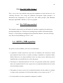
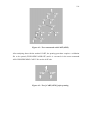
The principle of finding the most compatible partition is based on the construction of a
lattice graph with the following shape :
Fig 2. Example of a lattice graph
6
On this graph the initial partition S0 is made up of n individuals divided up into n1 points
labelled y1, n2 labelled y2, ... and nm points labelled ym. Using a criterion which will be
presented further on, SIPINA will determine the variable which gives the best possible
discrimination between points y1, y2, ... and ym, which is the same as determining the
variable which gives the most compatible partition with that brought about by the
endogenous variable Y. In this virtual example the variable which gives the best
discrimination is Xj.
SIPINA will now attempt to generate a new partition from that brought about by Xj. This
should be "better" according to the criterion presented below, and will be obtained by
segmenting the set of points for which Xj is equal to using the variable Xp. SIPINA again
attempts to find a new partition which is better than the present one. The chosen partition is
obtained by merge. SIPINA groups together two elements.
Once again, it is attempted to find a new partition. The process stops when no better
partition can be brought about by any process of merge and/or split.
The criterion for finding a new partition was built in accordance with certain mathematical
properties (Zighed, 1992) which it would take too long to present here. The expression of
this criterion is given below : Let St be the partition obtained at stage t and I(St) the value
of the criterion.
k
 n. j
I ( S t ) = ∑α .
j =1
 n
nij + λ 
nij + λ 
mλ
1
−
∑ n + mλ  n + mλ  + (1 − α ) n
i =1 . j


.j
j
m
Where :
- k is the number of elements in St={st1, st2, ..., stj, ..., stk}
- m is the number of modalities of Y
- n = Card(Ω1) = Card(St)
- n.j = Card(stj)
- nij = Card(ω ∈ stj / Y(ω) = Yi)
- α = 0.975 and could fluctuate between [0;1[ (Fusinter method)
and α=1 corresponds to the Fusbin method
- λ = 1 and could fluctuate between [0;+∞ [
The new partition St+1
St. That means
7
brought about by the process described above should be better than
I(St+1) < I(St).
For the quantitative variables, the discrimination points are determined based on the
Fusinter or Fusbin method Zighed (1995).
8
1.
General presentation of SIPINA_W

This section describes the SIPINA_W elements you may encounter during a work
session.
 environment
1.1. The SIPINA_W
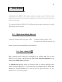
1.1.1.Starting SIPINA_W
To load SIPINA_W you double click on the SIPINA icon in the Windows program
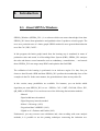
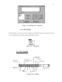
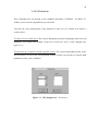
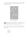
manager. You will see appear the SIPINA environment as shown in figure 1.1.
Figure 1.1 : SIPINA environment
The screen contains different elements that need to be specified. You immediately see the
empty SIPINA sheet which will enable you to store data. Furthermore you see the three
9
icons Graph, Classification Matrix and General Result that may be restored to comment the
results of an analysis.
Before explaining their function we shall describe the menus and, in the same context, the
toolbar.
1.1.2.Menus
1.1.2.1.File Menu
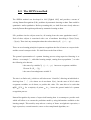
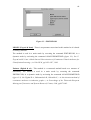
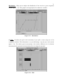
The first menu of the menu bar represents the file menu (figure 1.2).
Figure 1.2 : File menu
New
: Gives a new (empty) sheet.
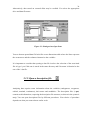
Open
: Loads existing SIPINA files (data files, parameter files and validation files)
stored on disk space through the medium of the dialogue box Open (figure 1.3).
Save
: Saves a file presently open in the SIPINA environment. If no information has
been saved yet the dialogue box Save As appears on the screen.
Save_As : Saves the file in use with the option that you may change the file name in the
dialogue box (figure 1.4).
Close
10
: Closes the open file. SIPINA eventually asks if the modifications of the file
should be saved or not.
Figure 1.3 : Dialogue box ‘Open Data’
Figure 1.4 : Dialogue box ‘Save As’
Import
: Loads files of type DBASE IV, Paradox and Lotus 1-2-3 through the
medium of the dialogue box Open Data.
Printer Setup : Specifies the configuration of the printer.
Print
: Prints the content of the selected element.
Exit
: Quits SIPINA and eventually asks if the modifications of the file should
be saved or not.
11
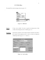
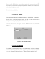
1.1.2.2.Edit Menu
The menu Edit is used to manage a data set (figure 1.5).
Figure 1.5 : Edit Menu
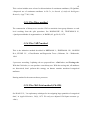
NewVar
: Creates a new variable. You have to specify the characteristics of that
variable in the dialogue box New Variable (figure 1.6).
Parameters
: Specifies the parameters of the analysis and the constraints associated to
the calculus of the production rules as well as to their use during the
validation procedure (figures 1.7, 1.8 and 1.9).
Figure 1.6 : New Variable
12
Figure 1.7 : Parameters / General
Figure 1.7 : Parameters / General
• Title : enables to give a title to your work session.
• Size : specifies the minimum size of a vertex. This constraint prohibits a partition
involving vertices with a size of observations below the chosen number. If you do not
select any size SIPINA_W proceeds with a default size = 5.
• Poisson Test, p-level : Specifies the use of a ‘stopping rule’ in the construction of the
tree. The aim of this test is to verify that the leaf can not be considered as a random
draw of the initial vertex. Pay attention by using it, it indicates more a gap to the
homogeneity that a causality (see Rakotomalala R., Zighed A., Rabaséda S.,
« Validation of rules issued from induction graph », in Procceedings of The Information
Processing and Management of Uncertainty in Knowledge-Based Systems - IMPU’96,
pp.1259-1264, Grenade, Juillet 1996).
• Chi-square test (split), p-level : it is the Quinlans stopping rule described in « Induction
of Decision trees », in Machine Learning, 1(1), pp81-106, 1986. The decision to split
occurs when the independence between modes of attributes and classes is rejected. It
13
seems that to insure the existence of a link, it is necessary to fix a weak critical risk (<=
0.001).
• Chi-square test (distribution), p-level : it is a test to insure that distribution of classes in
a leaf is different to the distribution in the whole learning sample. This test is used by
Clark and Niblett to avoid highly specific rules in the CN2 induction (see Clark P. and
Niblett T., « The CN2 induction algorithm » , in Machine Learning, 3(1), pp261-283,
1989).
Figure 1.8 : Parameters / Process:
Figure 1.8 : Parameters / Process
• Force Lambda to... : Enables to give a value to the parameter lambda which is needed
for the calculus of the ‘quadratic uncertainty measure’ (SIPINA method). If this
characteristic is not forced SIPINA_W optimises its value (see Technical Report
« Sipina Method », D.A.Zighed, R.Rakotomalala, at ftp://eric.univlyon2.fr/pub/publications).
14
• Force Alpha to... : Enables to give a value to the parameter alpha which is needed for
the calculus of the ‘quadratic uncertainty measure’ (SIPINA method with Fusinter
discretisation). If this characteristic is not forced SIPINA_W optimises its value.
• Automatic Pruning : For the C4.5 method, activates the pruning option which makes
you avoid to keep rules that are not reliable.
• p-value for pessimistic error : Specifies the critical p-value necessary to the calculus of
the pessimistic error rate used when including the pruning option in the C4.5 method.
• parameters for WDTaiqm : « Backward pruning » allows you to specify pruning
strategy during induction process. If it is not checked, method uses a stoping rule,
otherwise it performs a hurdling grow before pruning. « Complexity cost » is complexity
bias that you can introduce.
• parameters for MDL : « Theory cost » and « Exceptions costs » allows you to specify
trade-off between accuracy and complexity in Quinlan and Rivest strategy.
Figure 1.9 : Parameters / Rules :
Figure 1.9 : Parameters / Rules
15
• Size : makes SIPINA_W calculate its production rules considering a minimum
number of observations in the vertices.
• Specification threshold : makes SIPINA_W use a specification threshold.
• Only final vertex : This option makes SIPINA_W calculate the rules corresponding
exclusively to the final vertices; otherwise, the rules are generated for all the vertices.
• Intensity of implication : introduces the rules’ validation test based on the LERMAN
statistic, p-level is specified in General page (Poisson-test).
• Distribution gap : is the same as Chi-2 test Distribution. When the distribution of
classes in a node is not significantly different of the distribution in the learning sample,
we consider that rules are irrelevant. The p-level is specified in Distribution test
(General page).
• Digits : specifies the number of digits for the decimals.
• Global min : permits you to fix the minimum value of the intervals of discretisation.
• Selection : This option leaves you the choice which strategy (size, Bayes, jmeasure,
p-value, Bagging) will be used for the validation and the generalisation procedures,
when two or more rules leading to different decision can classify the same case
1. Size : number of examples covered by the rule;
2. Bayes : estimation of accuracy rate;
3. j-Measure : an indicator proposed by Goodman & al. (see GOODMAN R.M.,
SMYTH P.(1988), « Information-theoretic rule induction » , Proceedings of the 1988
European Conference on Artificial Intelligence, Pitman: London.);
4. p-value : corresponds to the intensity of implication. This indicator is derived from
the Lermans statistic (see Poisson-Test);
5. Bagging : it is the bootstrap aggregating predictor developped by L.Breiman. see
« Bagging Predictors », L.BREIMAN, Technical Report 421, Departements of
Statistics, University of California, September 1994. The idea is to choice the class
having the plurality on the rules activated.
16
Copy Data : Copies data to the Windows’ clipboard.
Remark : The commands Copy / Paste may have the attributes data, graph, results and
matrix depending on the active element after an analysis.
Paste Data : Pastes data after a copy data
Delete
: Deletes a Row or a Column in the SIPINA data matrix.
Insert
: Inserts a Row or a Column in the SIPINA data matrix.
Recode
: Specifies the discretisation method that is used if during a work session you
include continuous variables in your model (figure 1.10).
Figure 1.10 : Recode
17
1.1.2.3.Analysis Menu
The analysis menu is used to execute data analysis (figure 1.11).
Figure 1.11 :Analysis Menu
Automatic
: Accomplishes automatically the analysis of your data. In this case,
induction method tries to find the best possible partition.
Split
: Enables a partition in an interactive mode (Figures 1.12 et 1.13).
Merge
: Enables a fusion in an interactive mode (Figures 1.12 et 1.13).
Continue
: In the case of interactive mode this command makes the analysis
switch to automatic mode which finishes the analysis (Figures 1.12 et
1.13).
18
Figure 1.12 : Dialogue box ‘Restrictions’
Figure 1.13 : Dialogue box ‘Restrictions’
Cross-validation : When the available data contains a few cases (less than hundred), it is
more efficient to use cross-validation for evaluate rules. (see for
complete information: Stone M.(1977), « Cross-validation: a review »,
Math. Operationforsch. Statist. Ser. Statist., 9:127-139.). The principle
is simple. The sample is divided in v subsets (L1, ..., Lv). For every j
(j=1..v), (L-Lj) becomes the learning sample on which we apply the
procedure, and the validate file is the Lj_th sample. When you select
this option, a dialog box will appear asking you to fix the number of
subsets and the sampling mode. ‘V-fold’ is the number of data parts
you want and ‘sampling’ reflects the method used to create these parts.
The number of data parts may vary between 1 and 10 (Figure 1.14).
19
It seems that stratification give more accurate results (Breiman and al.
Classification and regression trees , Chapman & Hall, 1984, pp245247). Results are recorded in a summary table indicating: the rate of
well-classified, the size of learning sample, the size of validation
sample and the number of cases unclassified by rules. The knowledge
bases (rules) corresponding to each processing is saved in files
similarly name that the datafile, but with extensions (.K1 ... .Kv).
Figure 1.14 : Dialogue box ‘Cross-validate parameters’
Bootstrap:
This is a method of sampling proposed by B. Efron.
The principle is to make x randrom draw with replication in the
learning sample. On each subset, we apply the induction algorithm,
and produce a knowledge base system (K1..Kx).
One of applications of this strategy is to merge all the knowledge base
[knowledge based system K1..Kx are merged automatically in KBA],
and apply the bagging predictor for generalisation or validation on a
test sample. A dialog box (Figure 1.14b) allows you to specify number
of replication (range : 1..99).
Figure 1.14b : Dialogue box ‘Replication’
20
Multiple test:
This strategy performs several trials on one dataset.
Dataset is divided in learning sample (xx%) and test sample (100xx%). We can repeat m times this process with a fixed randseed value
for each induction methods. So, we obtain a paired sample which
allows us to use a more powerfull test in quantitative comparison of
algorithms (e.g Student's matched paired test).
When we divide dataset, sampling can be stratified (according to class
attribute) or not.
You can fix size of training set, trials and sampling method (Figure
1.14c).
Figure 1.14c : Dialogue box ‘Multiple test parameters’
Pruning
: Enables you to apply the pruning procedure when using the C 4.5 and
CART methods. We note that this procedure corresponds to the learning
step when using C 4.5 and acts on the validation step when working with
CART.
21
Go back to : At the final partition you may decide to delete some executed operations
until you reach a certain level (vertex) where you will continue your analysis
(figure 1.15).
Figure 1.15 : Dialogue box ‘Go Back To…’
Method
: This command is needed to specify the method of analysis and the
discretisation method for SIPINA (Figure 1.16).
Figure 1.16 : Dialogue box ‘Method of analysis’
Stop analysis : Stops the current analysis followed by the deletion of the graph.
22
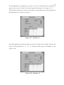
1.1.2.4.View menu
Figure 1.17 : View menu
Path of the individuals : Shows in which vertex an individual is positioned for a given
level (figure 1.18).
Figure 1.18 : Path of Individuals
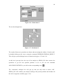
1.1.2.5.Window Menu
In the Window menu you can use the Cascade and Tile commands to rearrange the SIPINA
windows so that all running applications are visible on your desktop. Moreover you can
arrange the application icons and you can switch to one of the four SIPINA applications
(figure 1.19).
23
Figure 1.19 : Window menu
1.1.2.6.Rules menu
The rules menu enables to work on validation and generalisation files (figure 1.20).
Figure 1.20 : Rules menu
File
: Gives the dialogue box to open a rule file.
View
: Shows the rules extracted from the lattice graph (figure 1.21).
Export
: Export rules into another KBS format (Prolog and SelfMind)
24
Compute : Computes the production rules of the work session.
Add
: Enables to add your own rules (Figure 1.22).
Simplify : Simplifies a rules file (full, recover and like C4.5).
Merge
: Merges two or more KBS if these files uses the same variables.
Evaluate : Enables you to calculate the characteristic results of the rules (1-error rate, size,
jmeasure, 1-p-value) when introducing the rules manually.
Validate : Tests the power of the computing production rules.
Generalisation : is used to make forecasts on a data set for which the observations
concerning the endogenous variable are not available.
Copy
Cut
Paste
Print
Figure 1.21 : View Rules
25
Figure 1.22 : Dialogue box ‘Add rules’
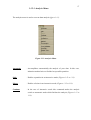
1.1.2.7.Help Menu
The help menu covers most of the explanations described in the user’s manual (Figure
1.23). Furthermore, it is possible to get information by topics.
Figure 1.23 : Help Menu
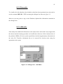
1.1.3.The Toolbar
Information
first vertex
Var Icon :
To create a new
variable
Folder Icon :
To open a file
Disk Icon :
To save a file
Graph pen
Graph brush
Follow Icon :
Path of the
individuals
Split
Merge
Continue
Figure 1.24 : Toolbar
Graph font
26
The toolbar (figure 1.24) enables you an immediate access to some of the SIPINA_W
commands and it incorporates some useful instruments to edit the lattice graph and the
fonts.
The windows presented in the following sections may be activated by choosing one of
them with the command WINDOW or by double clicking on the corresponding icons.
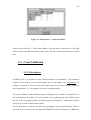
1.2. The sheet
The sheet represents a two dimensional table where data is put (Figure 1.25).
Figure 1.25 : The SIPINA sheet
1.3. The graph
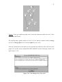
The induction graph (figure 1.26) visualises the results of the learning procedure
concerning the operations that have been executed on the initial population.
Each box reflects a vertex in which the number of cases for the given modalities are
shown. You can also see the address of the vertex at the left of it, i.e. the position of the
vertex in the hierarchy of the constructed induction graph. The address [ i , j ] means that it
is the jth vertex at the ith level.
27
The modalities of the endogenous variables are only shown at the right of the initial vertex.
The links between vertices visualise the evolution from one state of being of the partition
to another. Furthermore, concerning the split operation the name of the variable which
enabled the segmentation of a vertex is shown, as well as the modalities of this variable on
which the vertices below are based upon.
A better visualisation of the graph is possible when moving the vertices with the mouse.
Moreover, the colours of the vertices’ border and background and the character’s font used
in the graph may be modified.
level number
vertex number
size of class one
size of class two
name of the variable used for
operation n°1: Split
state of the variable colour that
enabled the split of vertex 1,1.
Figure 1.26 : Graph Window
28
1.4. The classification matrix
The classification matrix shows you how the SIPINA_W analysis can forecast the
modality of the endogenous variable for an observation. To do so, we must consider the
specification threshold which determines the conclusion in each vertex of the final
partition.
In each final vertex you note the modality that is the most present relatively to the total
number of cases reflected in the vertex.
If this ratio exceeds the specification threshold it is considered that this modality of the
endogenous variable belongs to all observations of this vertex.
On the contrary, if the ratio is below the specification threshold the result of the analysis is
called unclassified, i.e. the procedure could not conclude in a significant result.
The classification matrix shown in the window (figure 1.27) is explained as follows :
• The columns represent the modalities of the endogenous variable forecasted by
SIPINA_W and the possible unclassified characteristic.
• The rows reflect the real observations concerning the endogenous variable.
• In a cell you can see the cases for which SIPINA_W forecasted a certain
modality of the endogenous variable, knowing its real modality.
Above the matrix itself you can see two more results :
29
* The specific accuracy rate reflects the ratio of observations (in %) that were well
classified without considering the unclassified cases.
30
• The unspecific accuracy rate gives an analogous ratio which considers the
unclassified results.
Figure 1.27 : Classification Matrix Window
1.5. The general result
The general result window (figure 1.28) shows each partition resulting from a
SIPINA_W operation (split, merge). The operations are numbered considering their
occurrence and they may be visualised using the scroll bar.
Figure 1.28 : General Result Window
31
For each operation you get information on the following elements:
• The number of the operation
• The operation leading to the partition
• The name of the variable on which has been operated
• The address of the vertex on which has been operated
• The relative gain in uncertainty. This amount is the relative difference (in %)
between uncertainty before operation and uncertainty after executing the
operation.
• The partition resulting from the operation. This is shown as a table giving the
vectors of occurrences (modalities) for each vertex existing after the operation.
These results give you the possibility to reconstruct the SIPINA_W analysis step
by step and to understand the reason for the realisation of an operation.
1.6. Selecting a vertex
You may get more information on a vertex by selecting it (click with left mouse button)
followed by a click with the right mouse button. The dialogue box as shown in figure 1.29
appears:
Vertex : Visualises the vector of the selected vertex, i.e. the number of individuals having
the characteristic Yi of the endogenous variable. This holds for all the modalities
of the endogenous variable (figure 1.29).
32
Figure 1.29 : Dialogue box ‘Information on Vertex - Vertex’
Elements
: Shows the individuals contained in the vertex and their identification
number or identification name (figure 1.30).
Figure 1.30 : The dialogue box Information on Vertex - Elements
Distribution
33
: Helps you to analyse the distribution of the cases for a given exogenous
variable (figure 1.31), numerical informations (average, STD...) are
provided when attributes is continuous.
Figure 1.31 : Dialogue box ‘Information on Vertex - Distribution’
where:
: Copy to the clipboard as a bitmap
: Copy to clipboard as
: Print the chart
: Diagonal bar chart
: Horizontal bar chart
: Vertical bar chart
: Curve
: Smoothed curve
: Switches between 3D and 2D views
: Rotate
: Profoundness
: Edits legend
text
34
: Vertical grid pattern
: Horizontal grid pattern
: Edits title
: Changes police
: Tools
: Changes chart options
Gain : Visualises the gain in the uncertainty if you split a vertex using one of the
exogenous variables. This information is very useful during a ‘step by step’ work
session
(figure 1.32).
Figure 1.32 : The dialogue box Information on Vertex - Gain
35
2.
Data Editor
Analysing data with SIPINA_W requires opening or creating a data set. The first section
of this chapter describes how to open an existing data set. The data set creation is the object
of the second section.
The examples included in SIPINA_W will illustrate the presented explanations, for quick
familiarising with the program.
2.1. Open an existing data set
A data set is characterised by two types of files:
- a data file with the extension *.dat ;
- a description file with the extension *.par.
Starting a work session requests that you open both files.
2.1.1.Open a data file
Data is generally stored in data files, recognisable by the attribute .dat. You can start
SIPINA_W by opening a data file from the SIPINA File menu: File/Open/Data, or by
clicking on the folder icon in the toolbar.
The dialogue box appearing enables you to choose a data file from the listed file names
with the extension .dat (Figure 2.1). File Open relates you automatically to a SIPINA subdirectory: C:\SIPINA\EXAMPLES. If a data file has been placed elsewhere, the subdirectories of C:\ can be freely chosen.
36
Alternatively, data stored on external disks may be recalled. You select the appropriate
drive and data file name.
Figure 2.1: Dialogue box Open Data
You see that an opened data file looks like a two dimensions table where the lines represent
the occurrences and the columns characterise the variables.
It is important to consider that opening a data file involves the selection of the associated
file of type *.par if this one is stored in the same directory and if its name is identical to the
one of the *.dat file.
2.1.2.Open a description file
Analysing data requires some information about the variables (endogenous, exogenous,
ordinal, nominal, continuous), their name and modalities. The description files (*.par)
contain such information, respecting the description file structure (as shown in the syntactic
map). You can open description files by different procedures. Your choice of procedure
depends on what you want to know and/or to do.
37
2.1.2.1.Analysing data needs recalling a description file
Between work sessions, data is stored in data files. When you open a data file, the
associated information enabling analysis have been reinitialised, i.e. you will have to open
the description file after opening the data file to recall the particular information of the
data set. If the associated file is stored in the same directory as the data file and if its name
is the same as the name of the data file, then this action is executed automatically by
SIPINA_W©. You have to select manually a description file after opening a data file if one
of these conditions is not true. To do so, use File/Open/parameters and enter the file
name in the dialogue box (this action is similar to the one concerning File/ Open/ Data).
This will add the name of the variables, as well as the name of the cases (if specified) to the
data set, and establishes the link between the data file and the description file.
2.1.2.2.Content of a description file
You may visualise the content of a description file in a SIPINA data matrix (the syntactic
map) to get information that helps you choose the adequate parameters for your analysis.
You should do this before you open a data file as the result of the visualisation procedure
replaces all contents of the data matrix. After execution of File/Open/Data, you select a
file name (click on that name in the list) and you replace the extension .dat by .par.
Look always out that your data set is saved before opening any other file.
For practical reasons, we suggest a visualisation of the description files in MS-WORD, for
instance.
38
2.1.3.Illustration
! You open the data file EV2.dat by clicking on the folder icon, or by selecting
FILE/OPEN/DATA, followed by a double-click on the file name in the dialogue box. A
data matrix appears, as shown in Figure 2.2.
Figure 2.2 : Data in the Sheet
In this table, the endogenous variable represents a certain type of alcohol (column TYPE)
as Mirabelle, Poire or Kirsch. This variable is qualitative, nominal and is coded as follows :
- KIRSCH=1 ;
- MIRABELLE=2 ;
- POIRE=3.
The exogenous variables characterise different rates of the chemical components of these
three kinds of alcohol. This way you have nine exogenous variables : MEOH, ACET, BU1,
BU2, ISOP, MEPR, PRO1, ACAL, SOM.
39
Once the data appeared, you may immediately realise that the whole set of exogenous
variables is quantitative. Nevertheless, the SIPINA method is compatible with the use of
qualitative exogenous variables.
! It is possible to visualise immediately a subset of information of the description file
once you opened the data file. To do so you double click on the variable name shown in the
first line of the data matrix.
For example, a double click on the variable name MEOH makes appear the dialogue box as
in figure 2.3.
Figure 2.3: Structure of a variable
The information shown tells you that the variable is exogenous, continuous and takes its
values in the interval [0 , 2].
! To strengthen the importance of the description file, you may move the file name with
the extension .par
to another directory before opening the corresponding data file.
Recalling EV2.dat then shows you the same data matrix as in the beginning but without the
variables names. This means you only got the data and you do not have any information
concerning the variables or the parameters.
40
In this case the data file did not find the corresponding description file. You cannot
perform any analysis until a description file has been opened. Therefore you have to open
the description file EV2.par; this will add the missing information.
2.2. Create a data set
Data you want to analyse do not always appear in «ready for use» files. It happens that you
have to create your own file if, for example, data work with only exists on paper reports. In
this case, SIPINA_W enables you to create a data set and you can store it in a file. Of
course, this action may be executed by some other editors and the files (containing data)
may be imported by SIPINA_W (see section 2.3.).
2.2.1.SIPINA_W Editor
As data analysis in SIPINA_W requires data with a certain structure, using this editor to
create a data set involves that this condition is verified.
The first step of creating a data set is characterised by the necessity of an empty data sheet.
The command FILE/NEW makes appear such a sheet, as shown in figure 2.4.
The creation of a data set in SIPINA_W is explained in four more steps: structure
definition, variables status, data input and case identification.
Figure 2.4: FILE/NEW
41
2.2.1.1.Structure of a data set
2.2.1.1.1.Giving a title to your analysis
The structure of a data set is defined by two elements. First, you may give a title to your
analysis on the data set. This information is a complement to basic information but it is not
necessary. This means if you do not specify a title your analysis will not be altered at all.
As the title helps you defining the data set, it appears in the description file, respecting the
syntax of the syntactic map.
When creating a data set you may specify a title by activating the command
EDIT/PARAMETERS (showing a dialogue box as in figure 2.5) where you enter the title
name in the TITLE field.As you can realise this dialogue box contains above all
information on the parameters required for the analysis. The function of these will be
explained in chapter 3.
Figure 2.5: EDIT/PARAMETERS
2.2.1.1.2.Defining your variables
The second element characterising the structure of the data set is of course reflected by the
variables definition. When analysing data you want to explain a specific feature and to do
so you need to consider some other features. This places us in the case of modelisation
42
where
43
the information you want to explain is called the endogenous variable and the variables that
may be conclusive in the explanation are defined as exogenous. At this level the difference
of these types of variables, or the variable status will not interfere in this section. The only
interest here lies in the statement whether a variable is qualitative or quantitative.
Some variables generally define a state of being as, for instance, the sex of a person is
either male or female. We characterise them as qualitative variables.
A qualitative variable may also represent a classification of a quantitative variable, i.e.
its respective states are, for example: below 5°C, between 5°C and 25°C and finally higher
than 25°C. The qualitative variable in this example just regroups all the cases of the
respective quantitative variable. Moreover you may define these states as cold, medium and
hot.
In SIPINA_W, such states are called modalities.
You may also use quantitative variables in your analysis; these variables reflect the result
of a measure. To get back to the temperature example, the quantitative variable includes all
the different observations of temperature. This kind of variables can be used because
SIPINA_W
 automatically discretises them when executing its analysis. Furthermore,
you may apply such a discretisation in SIPINA_W before any analysis; discretisation
means grouping a number of classes.
Figure 2.6: EDIT/NEWVAR
44
45
Defining variables in SIPINA_W is achieved by the command EDIT/NEWVAR which
provides the means to specify the variable. You may also click on the Var icon.
In the dialogue box (figure 2.6) you see different fields:
"
In the NAME field you have to enter the name of the variable, limited to 255
characters. To do so you can click on the field, or you can move around in the box by using
the Tab, and you type the name.
"
You also have to define sequentially the modalities of the variable, considering the
syntax Modality_name=Value, where the values 1,2,3,…have to be taken. The
corresponding field is the MODALITIES field. Then you click on the ADD button to keep
this modality.
This procedure is executed until you entered all the modalities. To exclude a modality from
the list, you select it with the mouse in your list, then you click on the REMOVE button in
the box.
"
To select the type of the variable, in the TYPE field you click on the corresponding
cell.
" The STATUS field is similar to the type field: See section 2.2.1.2. Variables Status.
Defining the type and the modalities of a variable requires some more explanation on
qualitative and quantitative variables in the context of SIPINA_W
:
" In the case of a qualitative variable it may be ordinal or nominal :
Ordinal : This means the variable has already been grouped into classes and
SIPINA_W decides freely of the union of different classes if they do
not seem to be significant.
46
47
Nominal: As in the example of a persons sex, no grouping is possible. Even if a
class is not significant, SIPINA_W will not try to unify classes.
The ordinal type is set by default in SIPINA_W and for every nominal variable, when
you start a work session, you have to adjust the type position.
" When facing a quantitative variable, you have to define artificially its modalities. This
is done automatically by choosing the continuous type, where MINI=0 and MAXI=999,99.
Of course, you may enter the modalities manually to specify the extremes.
Remark: You should not use MINI or MAXI as modality names of a variable because these
are default expressions for the continuous type in SIPINA_W.
Once you finished the input of the elements necessary for the creation of a new variable
you validate the information by clicking on the OK button. SIPINA_W creates then a
column which has as first line (and not as first case) the name of the variable you defined.
2.2.1.2.Variables status
We explained so far how to define a variable without specifying how to select the status of
the variable. This step is necessary for the creation of a variable.
The aim of this section is to reveal the distinction between an endogenous, an exogenous
and a variable with the status ‘not include’ in the context of SIPINA_W.
"
An endogenous variable is a variable you want to explain. The modalities of this
variable can be forecasted by SIPINA_W which builds a model based on exogenous
48
variables. The endogenous variable has to be qualitative and its modalities, submitted to
the general syntax, have to take the values 1, 2, and so on.
"
An exogenous variable may contribute to determine the behaviour of the endogenous
variable. It can be qualitative or quantitative.
"
Generally, all variables are included in the model but if you assume that a specific
variable does not contribute at all, or marginally to an adequate forecast, you may decide
not to include this variable in the analysis. In this case you select the status option ‘not
include’ in the dialogue box following the command EDIT/NEWVAR (see figure 2.6).
2.2.1.3.Data input
We should now concentrate on how data is entered in the SIPINA sheet. The sheet, as
presented in the beginning of this chapter, is empty and data entry is of course preceded by
the variable definition.
The matrix is in selection mode by default, i.e. no cell is to be altered. The commands
Copy, Paste, Insert and Delete are linked to this mode.
Data entry with the keyboard is possible once you switch to the editing mode. This mode
is activated by pushing F2 or Return, or directly by typing your data in the selected cell.
You use Return to terminate data entry for one cell or you immediately move to the next
cell with the directional arrows.
This recalls automatically the selection mode. You realise that rows are added as long as
you move downwards. If more than one variable are defined you may also move to the
right (left). All the variables have the same number of cases (rows).
49
# Copy and Paste Data: You may however copy data, selected from the SIPINA sheet or
from another program’s spreadsheet to the SIPINA sheet. this procedure is also
applicable to copy data from SIPINA_W to another spreadsheet. A restriction of the copy
command is that the selected cells have to form a rectangular block. Once the data cells
selected (with the mouse or by Shift+Arrows) use the command EDIT/COPY. Then you
choose the cell where you want to place the upper left cell of the block and you use the
command EDIT/PASTE.
# Insert and Delete: Still in selection mode, you may delete rows (columns) [one at the
time] with the command EDIT/DELETE/ROW(COLUMN). Of course one can add rows or
columns with EDIT/INSERT. When you insert a column, however, the variable definition
dialogue box appears automatically.
Both commands take the selected cell as reference for the corresponding row or column.
2.2.1.4.Case identification
SIPINA_W gives a number to every case as its default label (its occurrence).You may
change this label to save more specific information concerning an observation. The new
label appears every time the occurrences are listed.
The appropriate action to change labels is given by double clicking on the cases’ label (in
the very first column). A dialogue box as in figure 2.7 pops up where you enter the new
label.
Figure 2.7: Changing the label of a case
50
You accomplished data entry and to keep all the information you have to save the data set,
using the command FILE/SAVE_AS or by clicking on the disk icon in the toolbar.
2.2.2.Illustration
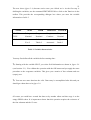
The following table shows a data set we want to analyse (table 1).
- The variable SPOT reflects the state of having skin spots caused by beard growth. The
modalities are: to have skin spots (yes=2), not to have skin spots (no=1).
- The variable HAIR is characterised by the thickness of the hair, (soft=1) and (thick=2).
- The variable GROWTH gives the beard growth in millimetres per day.
- The variable COLOUR points at the fact whether the beard is (bright=1) or (dark=2).
SPOT
HAIR
GROWTH COLOUR
1
1
10
1
1
1
10
1
1
1
10
1
1
1
9
1
1
1
8
1
1
2
1
1
1
2
3
1
2
1
2
1
2
1
8
2
2
2
8
2
2
2
9
1
2
2
10
2
2
2
9
1
2
2
10
2
2
2
9
1
Table 1
51
The new sheet (figure 2.4) becomes active once you clicked on it. As the first step is
defining the variables, use the command EDIT/NEWVAR or click on the Var icon in the
toolbar. This provides the corresponding dialogue box where you enter the variable
information of table 2.
NAME
SPOT
HAIR
GROWTH
COLOUR
STATUS
Endogenous Exogenous
Exogenous
Exogenous
TYPE
Nominal
Continue
Nominal
MODALITIES No=1
Yes=2
Nominal
Soft=1
Thick=2
Bright=1
Automatic
Dark=2
Table 2: Variable characteristics
You may first define all the variables before entering data :
"
Starting with the variable SPOT, you select field information as shown in figure 2.8
(read section 2.1.). You validate the operation with the OK button and you apply the same
procedure to the exogenous variables. This gives you a matrix of four columns and one
(empty) row.
"
You can now enter data into the cells. Data entry is accomplished after this and you
should get a data sheet as in figure 2.9.
Of course you could have created the data set by another editor and then copy it to the
empty SIPINA sheet. It is important to know that this operation requires the existence of
the four columns and the 15 rows.
52
Figure 2.8 : Defining the endogenous variable
Figure 2.9 : SIPINA sheet containing data
Now you can save the data set : FILE/SAVE_AS or click on the disk icon and you choose
the file name, the directory where you want to store it and the drive.
53
2.2.3.Other Editor
You can also create a data set with another editor. Nevertheless you must respect the syntax
of the two files that constitute a data set :
- data file
- description file
This alternative requires however the creation of a text file containing the observations of
the different variables defined in the description file. The file has to look like a two
dimensional table where the rows contain the cases, and the columns characterise the
variables except for the first column representing the case identification. Data
corresponding to the different cells has to be separated by a space or a tab.
2.3. Import files
It is possible to import data from data base software, as for instance Paradox and DBASE.
In this case, we can open the file by activating the menu FILE/IMPORT, but the structure
of the data set has to be defined. To do so, refer to the paragraph create database.
When importing Lotus (*.wks) files, the labels (names) of the variables may be loaded
automatically. Nevertheless, all the variables are loaded as if they were continue variables.
Therefore, you have to redefine the status and the modalities of the non-continuous
variables by double clicking on the variable names in the SIPINA sheet.
54
3.
Learning
3.1. Default method : SIPINA
3.1.1.Basic Elements
In SIPINA_W the default method that is used is the SIPINA method.
As we indicated in the beginning of the user’s manual this analysis technique consists in
dividing the original population in several groups so as to explain the endogenous variable.
To facilitate the control of the analysis the program builds an induction graph which
visualises the production rules generated by SIPINA.
In this way the graph represents the different steps of the analysis and at each level several
vertices are represented. Moreover there exist links between different vertices on different
levels.
A vertex is part of a population partition where observations verifying the same criteria
(relative to the exogenous variables) are assembled, a partition being a gathering of final
vertices, i.e. vertices that are not linked to a lower level vertex.
In a vertex SIPINA gives a vector including the different cases corresponding to the
modality yi of the endogenous variable; this way the vertex represents all the modalities of
the endogenous variable. The aim of SIPINA is to create vertices in which the observations
55
correspond exclusively to one modality of the endogenous variable. We note that every
vertex is identified by its level number, the associated vertex number and its effective.
A vertex that is linked to another one means that the upper level vertex has involved the
lower level by the intermediate of a basic SIPINA operation. The basic operations are
described in the following section. (see Technical Report : D.A.Zighed and
R.Rakotomalala, « Sipina Method » at ftp://eric.univ-lyon2.fr/pub/publications).
3.1.2.Criterion to Optimise and Basic Operations
3.1.2.1.Criterion to Optimise
To bring the analysis to a successful conclusion SIPINA optimises a function which
measures a partition’s homogeneity. This function is the Quadratic Uncertainty Measure :
 n. j
I ( S t ) = ∑ α .
j =1
 n
k
nij + λ 
nij + λ 
mλ
∑ n + mλ 1 − n + mλ  + (1 − α ) n
i =1 . j


.j
j
m
(Fusinter)
or
k n
.j
I ( S t ) = ∑
j =1  n
m
nij + λ 
nij + λ 
1 −

n. j + mλ 
. j + mλ 
∑n
i =1
(for Fusbin, as α=1)
Where :
- k is the number of elements in St={st1, st2, ..., stj, ..., stk}, i.e. the final vertices
- m is the number of modalities of Y
- n = Card(Ω1) = Card(St)
- n.j = Card(stj)
- nij = Card(ω ∈ stj / Y(ω) = Yi)
- α = 0.975 and could fluctuate between ]0;1[
- λ = 1 and could fluctuate between [0; +∞[
56
3.1.2.2.Split
At a given step of the analysis, SIPINA gives you a measure of uncertainty for every final
vertex. The state of the partition will be altered by trying a new partition on the final
vertices.
To do this, you sequentially select the exogenous variables on which this new partition will
be based upon and you keep the split operation corresponding to the variable optimising
the gain of uncertainty; of course you have to be better off than before the operation, unless
you force the operation.
You may use the command split in the following cases:
- Analysis / Split
- Split icon
- Analysis / Automatic
- Analysis / Continue
The constraints you may include in your analysis leave you a large control on the
operations, as for instance the force option.
3.1.2.3.Merge
When merging two groups of individuals these have to be similar final vertices. At this step
of the analysis, considering all the final vertices, we test all the possible unions of these by
pairs.
The union of two final vertices optimising the relative gain in uncertainty is considered as a
merge. You do not execute the command merge if the relative gain is nil or negative.
57
The command may deteriorate the homogeneity of the sub-groups, but you have the
advantage of a limited number of vertices and their size of observations is reinforced.
The resulting production rules become more significant as the size stays relatively large.
You may use the command merge in the following cases:
- Analysis / Merge
- Analysis / Automatic
- Analysis / Continue
The manual command (Analysis / Merge) gives you the opportunity to operate and, at the
same time, to keep control on these operations by considering possible restrictions.
3.1.2.4.Continue
This operation makes SIPINA execute the standard operations automatically from a given
level of your analysis. The standard operations are summarised in the research of :
- merge
- merge-split
- split
This operation is activated by the command Analysis / Continue or during the automatic
running.
58
3.1.2.5.Go back to
This command does not belong to the standard operations of SIPINA. ‘Go Back To’
enables you to test some hypotheses on your model.
You may do so by deleting part of the analysis to start over at a certain level and/or a
certain vertex.
To start over at a certain level: The vertices depending on those belonging to that level will
disappear. You choose the number of the level in the list ‘level’ of the dialogue box
(figure 3.1).
To start over at a certain level and a specific vertex: The vertices depending on this vertex
will be deleted, as well as the corresponding analysis. In this case you have to specify both
parameters of the vertex’s address.
Figure 3.1 : The dialogue box : Go back to...
59
3.1.3.Discretisation methods
When using quantitative variables in your analysis, SIPINA_W discretises the variables.
This procedure is necessary to use them for segmentation. The variables are cut into
classes, creating few modalities and the generated variables classification is depending on
the capacity to explain the endogenous variable.
You can make global discretization, i.e before induction process all continuous attributes
are transformed into categorical variable, or local discretization i.e during tree growing
method searches dynamically best partition.
For global discretization, SIPINA_W gives you six alternatives of multi-valued
discretisation methods. Rules generated by RULE/COMPUTE use discetization
boundaries. The choice of the method is done by using the command EDIT/RECOD,
which shows the dialogue box as in figure 3.2. Some of them are available for dynamic
(local) discretization.
Manual discretisation: You will have to specify the boundaries of discretisation and this
is done in increasing order, separated by semi-colons.
Equal width intervals discretisation: You choose intervals with a similar width and the
parameter you insert is the amount of intervals.
Equal frequency intervals discretisation: Similar to the preceding case, you have to
select the number of observations in each interval.
Chi Merge (Kerber) : This discretisation method uses the Chi2 criterion in its calculus.
The parameter to enter is the critical risk associated to the tests, i.e. for a risk given at 5%
you enter 0.05. The method is used in a static mode by executing the command
EDIT/RECOD, in a dynamic mode by activating the command ANALYSIS/METHOD
(figure 3.3). See R. Kerber « Chimerge discretization of numeric attributes », in AAAI92,
San José, pp.123-128, 1991.
60
Figure 3.2 : EDIT/RECOD
MDLPC (Fayyad & Irani) : There is no parameter associated to this method as it is based
on entropy measure.
The method is used in a static mode by executing the command EDIT/RECOD, in a
dynamic mode by activating the command ANALYSIS/METHOD (figure 3.3). See U.
Fayyad and K. Irani « Multi-Interval Discretization of Continuous Valued Attributes for
Classification Learning », in 13th IJCAI, pp.1022-1027, 1993.
Fusinter (Zighed & al.) : This method is a contextual method based on a measure of
uncertainty. The method is used in a static mode by executing the command
EDIT/RECOD, in a dynamic mode by activating the command ANALYSIS/METHOD
(figure 3.3). See Zighed D.A., Rakotomalala R., Rabaséda S., « A discritization method of
continuous attributes in induction graphs », in Proceedings of the Thirteenth European
Meeting on Cybernetics and Systems Research, Vienna, 1996, pp997-1002.
61
Figure 3.3 : ANALYSIS / METHOD
Fusbin (Zighed & al.) : This method is a contextual method based on a measure of
uncertainty. But unlike Fusinter, Fusbin uses binary splits. This method is used in a static
mode by executing the command EDIT/RECOD. Moreover it is the default discretisation
method used by SIPINA. This option may be modified by the command
ANALYSIS/METHOD (figure 3.3).
Contrast (Van de Merckt) : See Van de Merckt T., « Decision Trees in Numerical
Attributes Spaces »,
in Proceedings of the 15th International Joint Conference on
Artificial Intelligence IJCAI-93, Morgan Kaufmann, 1993.
3.2. Other analysis methods
Parallel to the method SIPINA, there are other segmentation methods that may be used to
analyse a data set. The interest lies in the possibility to compare the results, for instance,
which enables you to apply the most appropriate method on data.
62
However, unlike SIPINA, these methods do not include the merge operation and they
involve their own discretisation techniques for quantitative variables; these techniques may
not be selected freely but are fixed.
We describe these methods here.
3.2.1.The ID3 method
This is the popular Induction Tree method introduced by J.R.QUINLAN : « Induction of
Decision Trees », in Machine Learning, 1, pp.81-106, 1986. You may associate it with a
Chi-square test stoping rule (split) when you have noisy data.
Choose the ID3 method by selecting the command METHOD in the menu ANALYSIS
(figure 3.7).
Figure 3.7 : To choose ID3 method
3.2.2.The C4.5 method
The method C4.5 differs from ID3 as the gain in uncertainty based on the Shannon
criterion is replaced by a gain ratio, and C4.5 proposes a pruning technique (See Quinlan
J.R., « C4.5: Programs for Machine Learning », Morgan Kaufmann Publishers, 1993).
63
This version includes new release for discretization of continuous attributes (J.R.Quinlan,
« Improved use of continuous attributes in C4.5 », in Journal of Artificial Intelligence
Research, 4, pp.77-90, 1996).
3.2.3.The Elisee method
The construction of binary trees uses the Chi2 to maximise inter-group distance at each
level resulting from the split operations. See BOUROCHE J.P., TENENHAUS N.,
« Quelques méthodes de segmentation », in RAIRO, 42, pp.29-42, 1970.
3.2.4.The CART method
This is the induction method described in BREIMAN L., FRIEDMAN J.H., OLSHEN
R.A., STONE C.J., « Classification and Regression Trees », Belmont, CA : Wadsworth,
1984.
2 processes according 2 splitting rule are proposed here : Gini Index, and Twoing rule.
With the Gini index, we can produce a non-binary tree. With the twoing rule, all attributes
are discretized, don’t perform this strategy on dataset contains unordered categorical
attributes.
Pruning method is the same on theses processes.
3.2.5.The Chi2-Link method (ChAID)
See KASS G.V., "An exploratory technique for investigating large quantities of categorical
data", in Applied Statistics, 24(2), 1975. We only use adjusted Chi-Square measure (pvalue).
64
3.2.6.The QR_MDL Method
This is one of the first methods using bayesian foundation to built decision tree. See
« Inferring Decision Trees using the Minimum Description length principle », in
Information and Computation, 80, pp.227-248, 1989. MDL principle (with Minimum
Message Length MML of Wallace ) is now very popular.
3.2.7.
The WDTaiqm method
This method is proposed by Louis Wehenkel. He introduce complexity bias during tree
growing and pruning. See « Decision tree pruning using an additive information quality
measure », in Uncertainty in Intelligent Systems (Bouchon-Meunier, Valverde and Yager,
eds), Elsevier-North Holland, pp.397-411, 1993.
 capacities
3.3. SIPINA_W
The present version of SIPINA_W has several limitations :
• A qualitative variable cannot have more than 10 modalities; this restriction is based
upon statistical criteria. In fact, a variable exceeding 10 modalities is considered ‘badly’
defined. Moreover, too many modalities involve too many vertices which may not be
significant due to an insufficient size of the sub-groups.
• The analysis is technically limited to 25 levels. We generally consider that a partition
that is not completed after 25 levels, is quite close to completion and therefore its results
stay interesting to analyse.
• The number of vertices at one level is technically limited to 50, the number of variables
in a data set has a maximum of 16384 and the number of cases cannot exceed 232 - 1.
• It is not possible to work on quantitative endogenous variables.
65
3.4. The two running modes of SIPINA_W
In SIPINA_W two working modes are available. Actually, you may proceed in your work
session either by the automatic procedure or by the interactive mode which leaves you
some flexibility concerning data manipulation.
3.4.1.Automatic analysis
The automatic running mode corresponds to a simple way of analysing data. To do so you
only need to activate the menu command ANALYSIS/AUTOMATIC and SIPINA_W
will build the entire model.
In fact, this command is identical to a succession of commands CONTINUE until no other
operation is possible, or if you reached the SIPINA_W capacities limit.
Remark: concerning the method SIPINA, the reasoning at each step of an analysis is
reflected by the algorithm shown in Appendix II. It is important to remember that the other
analysis methods do not include the merge of vertices operation.
Moreover, the analysis operation may be aborted by clicking on the button ‘Annuler’ in the
cancel window.
Finally,
to
cancel
an
analysis
you
have
ANALYSIS/STOP_ANALYSIS.
3.4.2.Step by step running
to
use
the
menu
command
66
This second mode of proceeding enables a large control on the operations. Indeed, at each
step of the analysis it is possible to choose the operation to be executed, and this
concerning the vertex and the variable of your choice.
In this way you are able to restrict the range of the study when using the commands
MERGE, SPLIT and CONTINUE. Actually, before executing the operation a dialogue box
appears, which enables you to choose the variable(s) to be activated as well as the final
vertex (vertices) that makes the operation effective.
To visualise the dialogue box enabling a restriction of the range of an analysis you activate
one of the commands MERGE, SPLIT or CONTINUE in the menu ANALYSIS. The same
results are produced when clicking on the corresponding icons in the toolbar (figures 3.8
and 3.9).
Figure 3.8 : Variable restrictions
Figure 3.9 : Vertex restrictions
67
Furthermore, this type of analysis leaves you the possibility to force an operation. This
option makes SIPINA_W execute the operation and optimise the model, even if the
forced operation involves a less good partition.
Remarks:
• All the final vertices and all the variables are active if no restriction has been specified.
• To select several contiguous elements you have to combine ‘Shift + (left) click’; noncontiguous elements require ‘Control + click’.
68
3.5. Results
During the analysis step some results on the data learning process may be visualised. The
different windows are:
- Graph window
- General result
- Classification matrix
- View rules
- Path of the individuals
3.5.1.Graph window
The induction graph (figure 3.10) visualises the results of the learning procedure
concerning the operations that have been executed on the initial population.
Each box reflects a vertex in which the number of cases for the given modalities are
shown. You can also see the address of the vertex at the left of it, i.e. the position of the
vertex in the hierarchy of the constructed induction graph. The address [ i , j ] means that it
is the jth vertex at the ith level.
The modalities of the endogenous variables are only shown at the right of the initial vertex.
The links between vertices visualise the evolution from one state of being of the partition
to another. Furthermore, concerning the split operation the name of the variable which
enabled the segmentation of a vertex is shown, as well as the modalities of this variable on
which the vertices below are based upon.
69
A better visualisation of the graph is possible when moving the vertices with the mouse.
Moreover, the colours of the vertices’ border and background and the character’s font used
in the graph may be modified.
Figure 3.10 : Graph Window
Remark : The window presented in this section may be activated by choosing it with the
command WINDOW/GRAPH or by double clicking on the corresponding icon. If you
execute the analysis this window is automatically opened to show the results.
At last, you may get more information on a vertex by selecting it (click with left mouse
button) followed by a click with the right mouse button. The dialogue box as shown in
figure 3.11 appears:
- Vertex (a)
- Elements (b)
- Distribution (c)
- Gain (d)
70
(a) Vertex: Visualises the vector of the selected vertex, i.e. the number of individuals
having the characteristic Yi of the endogenous variable. This holds for all the modalities of
the endogenous variable (figure 3.11).
Figure 3.11 : Information on one vertex
(b) Elements : Shows the individuals contained in the vertex and their identification
number or identification name (figure 3.12).
Figure 3.12 : Elements of one vertex
71
Distribution : Helps you to analyse the distribution of the cases for a given exogenous
variable (figure 3.13). This graph is most appropriate for continuous variables
Figure 3.13 : Distribution
d) Gain : Visualises the gain in the uncertainty if you split a vertex using one of the
exogenous variables. This information is very useful during a ‘step by step’ work session
(figure 3.14). The relative gain in uncertainty is the relative difference (in %) between
uncertainty before operation and uncertainty after executing the operation.
Figure 3.14 : Gain
72
3.5.2.General result
The general result window (figure 3.15) shows each partition resulting from a
SIPINA_W operation (split, merge). The operations are numbered considering their
occurrence and they may be visualised using the scroll bar.
For each operation you get information on the following elements:
- the number of the operation
- the operation leading to the partition
- the name of the variable on which has been operated
- the address of the vertex on which has been operated
- the relative gain in uncertainty. This amount is the relative difference (in %)
between uncertainty before operation and uncertainty after executing the operation.
- the partition resulting from the operation. This is shown as a table giving the
vectors of occurrences (modalities) for each vertex existing after the operation.
These results give you the possibility to reconstruct the SIPINA_W analysis step by step
and to understand the reason for the realisation of an operation.
Figure 3.15 : General result
73
Remark : The window presented in this section may be activated by choosing it with the
command WINDOW/GENERAL RESULTS or by double clicking on the corresponding
icon
3.5.3.Classification matrix
The classification matrix shows you how the SIPINA_W analysis can forecast the
modality of the endogenous variable for an observation. To do so, we must consider the
specification threshold which determines the conclusion in each vertex of the final
partition.
In each final vertex you note the modality that is the most present relatively to the total
number of cases reflected in the vertex.
If this ratio exceeds the specification threshold it is considered that this modality of the
endogenous variable belongs to all observations of this vertex.
On the contrary, if the ratio is below the specification threshold the result of the analysis is
called unclassified, i.e. the procedure could not conclude in a significant result.
The classification matrix shown in the window (figure 3.16) is explained as follows:
- The columns represent the modalities of the endogenous variable forecasted by
SIPINA_W and the possible unclassified characteristic.
- The rows reflect the real observations concerning the endogenous variable.
- In a cell you can see the cases for which SIPINA_W forecasted a certain modality
of the endogenous variable, knowing its real modality.
Above the matrix itself you can see two more results:
- The specific accuracy rate reflects the ratio of observations (in %) that were well
classified without considering the unclassified cases.
74
75
- The unspecific accuracy rate gives an analogous ratio which considers the
unclassified results.
Figure 3.16 : Classification matrix
Remark : The window presented in this section may be activated by choosing it with the
command WINDOW/CLASSIFICATION MATRIX or by double clicking on the
corresponding icon.
3.5.4.Path of the individuals
This
dialogue
box
(figure
3.17)
is
activated
when
using
the
command
VIEW/PATH_OF_THE_INDIVIDUALS; it shows all possible positions of the cases in the
induction graph. In this way you may see that, at a given moment of the analysis, a certain
observation X is positioned in the vertex i of level j.
76
Figure 3.17 : Path of the individuals
3.5.5.View rules
During a work session the command RULES/VIEW opens a window which contains the
rules that SIPINA_W has in its memory, whether they have been loaded or produced
during this session (figure 3.18).
You may print the rules or copy them to the Windows clipboard. Moreover, these rules
may be submitted to specific manipulations (see chapter 5).
77
Figure 3.18 : View rules
On the right of the rules you observe the first number in # # which reflects the rate of well
classified observations concerning a rule (1 - error rate). The second number between # #
is the number of cases corresponding to a rule (size). The third value between # # shows
the jmeasure that is to be maximised and the fourth value between # # is 1 - p-value
3.6. Illustration
The illustration of the preceding sections makes the object of this section and the examples
are related to the learning data base SPOT.DAT which has been described in chapter 1.
3.6.1.Automatic running
Figure 3.19 : Size = 1
78
Data manipulation is preceded by the specification of the parameters of the analysis. As
explained in section 3.1.4., you activate the menu command EDIT/PARAMETERS.
In this short example we advise you to enter a minimum size equal to 1, not to activate the
option ‘Poisson Test, p-level’ and to force λ=1 and alpha=0.975.
Figure 3.20 : α = 0.975 and λ = 1
Moreover, you enter a global minimum of 1 as the values of the quantitative variable
‘Growth’ are never below 1.
You may give any title you want to this analysis.
These specifications are reflected in the figures 3.19 -3.21.
Figure 3.21 : Global min = 1
Furthermore, this work session will use the software’s default method of analysis, i.e. the
SIPINA method and the discretisation technique FUSBIN.
At this step you may realise data manipulations. To do so you use the menu command
ANALYSIS/AUTOMATIC. The software then searches for the best possible partition. At
the end of the analysis you should see the following graph window:
79
Remark: If you get a different graph result, check the parameters and/or the cases in the
data matrix SPOT.DAT.
The resulting lattice graph contains six levels. You see that the software realised a merge
at level 6, a merge-split at level 4 and two splits at level 2 and 3.
After the visualisation of the graph you may generate the production rules reflected in the
graph. You use the menu command RULES/COMPUTE and the following window will
appear (figure 3.22):
Figure 3.22 : The dialogue box ‘View rules’
80
The first rule has the following meaning: If the colour of a person’s beard is bright (=1) and
if the hair is soft (=1) then we consider a certainty of 83% ( #0.83# ) that this person has no
spot problem. You can also see that this rule is true for 6 cases (# 6 #), the value of the
jMeasure is 0.1669 ( #0.1669# ) and the 1 - p-value is 0.828 ( #0.828# ).
Finally, when visualising the classification matrix and the general result, you get the
results shown below:
a.) Classification matrix (Figure 3.23)
Figure 3.23 : Classification matrix
Here, the ‘1’ in the first column and second row means that a person with no spot problem
has been classified as if he had spots. The specification threshold is 75%.
In our example, 93% of the cases have been classified correctly (as there are no
unclassified cases this is true for the specific and unspecific accuracy rates)
Remark : if the analysis had generated rules all true at 100% the classification matrix
would have been diagonal.
81
If you change the specification threshold (in this dialogue box) to 88% you will obtain the
figure 3.24 below :
Figure 3.24 : Threshold = 88 %
In this case, 7 persons have been classified as not having spots and the other cases got the
status ‘unclassified’. You then get a rate of well classified cases of 100% if the unclassified
cases are neglected (specific accuracy rate).
On the other hand, if you consider the unclassified elements the rate of well classified cases
diminishes to 46%, i.e. (7/15)*100, this result being not very concluding.
b.) General result (Figures 3.25 to 3.29)
In this example the first operation that has been executed on the initial vertex (population)
is a split using the variable ‘Colour’ with a relative gain in uncertainty of 6% (figure 3.25).
The vertex 2,2 (dark beard) includes 4 cases having spots and the vertex 2,1 (bright beard)
is composed by 7 persons without spots and 4 persons having spots.
If you visualise the dialogue box ‘Path of the individuals’ you can see that the vertex 2,2
concerns the cases 9,10,12,14 and the vertex 2,1 contains the other cases. The same result
is sequentially obtained if you select the vertex, click on the right mouse button and you
click on the folder ‘elements’.
82
Figure 3.25 : partition n°1
The second partition concerns the vertex 2,2 (dark beard) and the vertices 3,1 and 3,2
(bright beard - soft hair and thick hair) which were created by the split of vertex 2,1 using
the variable ‘Hair’; the relative gain in uncertainty is 8% (figure 3.26).
In the vertex 3,1 you have five persons without spots and one with a spot problem. The
vertex 3,2 contains 3 cases with spots and 2 cases without spots. At this level the vertex 2,2
has not been altered.
Figure 3.26 : Partition n°2
83
The third partition is resumed by the vertices 3,1 and 4,1 which has been created after a
merge of the vertices 2,2 and 3,2; the relative gain in uncertainty is 33% (figure 3.27).
This partition only has two vertices and it shows an uncertainty that is lower than that of
the partition at level 2 (also two vertices).
Figure 3.27 : Partition n°3
The fourth partition is got after the split of vertex 4,1 based on the variable ‘Growth’: the
vertices of this partition are 3,1 , 5,1 , 5,2 and the relative gain in uncertainty is 16%
(Figure 3.28).
Figure 3.28 : Partition n° 4
84
Finally, in figure 3.29, this partition contains the vertices 5,2 and 6,1 (after a merge of
vertices 3,1 and 5,1) and its relative gain in uncertainty is 31%.
Figure 3.29 : Partition n°5
3.6.2.Step by step running
A better comprehension of the analysis described in section 3.6.1. is possible if you try to
reproduce the lattice graph step by step. To do so we advise you to cancel the preceding
analysis by activating the menu command ANALYSIS/STOP_ANALYSIS.
You begin the step by step analysis with a split of the initial vertex. This may be done
when using the command ANALYSIS/SPLIT or you may click on the corresponding icon (
).
You then will see appear the ‘restriction’ dialogue box. You only need to click on the ‘OK’
button and the software searches automatically for the best possible partition generated by
the use of one of the active exogenous variables (figure 3.30).
85
Figure 3.30 : Partition n°1
You realise that SIPINA_W chose the variable ‘Colour’ to split the population into two
sub-populations (vertices):
- the cases with the characteristic ‘bright hair’ are situated in vertex 2,1;
- the cases corresponding to ‘dark hair’ are in vertex 2,2.
In the beginning of the analysis, data was represented by one sample of 15 cases in which 7
persons have spot problems and 8 persons do not have spots. As you have two sub-samples
now it is interesting to see if the split operation succeeded (more or less) in separating the
cases which have a different modality concerning the endogenous variable.
The visualisation of the classification matrix (figure 3.24), or the selection of the ‘Vertex’
folder in the dialogue box ‘Information on Vertex i of level j’ in both vertices, gives you
the following information: the first sub-sample includes the cases characterised by ‘bright
hair’, i.e. 11 persons where 7 cases do not have spots (figure 3.31); the second one contains
the observations corresponding to the characteristic ‘dark hair’, i.e. 4 persons and all of
them have spots (figure 3.32).
Figure 3.31 : Information on Vertex 1 of level 2
86
Figure 3.32 : Information on Vertex 2 of level 2
In this way SIPINA_W shows the relation between the colour of the beard and the
presence of spots, although this partition is not optimal. The conclusion may be
ameliorated, which requires a more detailed inspection of the vertices (left click on a vertex
to select and right click to get information).
Concerning the vertex 2,1 , the result in the folder ‘Gain’ makes you conclude that the use
of the variable ‘Hair’ diminishes uncertainty (figure 3.33):
Figure 3.33 : The dialogue Box ‘Information on Vertex 1 of level 2 / gain’
In an analogous way, if you analyse the distribution (folder ‘distribution’) of the variable
‘Hair’ in this vertex you see that modality 1 of the variable ‘Hair’ (soft hair) involves a
sub-sample in which almost all the persons do not have spots (figure 3.34).
87
Figure 3.34 : The dialogue Box ‘Information on Vertex 1 of level 2 / Distribution’
At this level of the analysis we invite you to produce the split operation on vertex 2,1 using
the variable ‘Hair’ (
).
The command ANALYSIS/SPLIT makes appear the dialogue box ‘Restrictions’ and you
choose the folder ‘Variables’ in which you click (select) on the variable name ‘Hair’
(figure 3.35). After that, you choose the folder ‘Vertices’ and you select level 2 and vertex
1, followed by a click on the ‘Add’ button (figure 3.36). This will give you the result
shown in figure 3.37 and the operation only acts on vertex 2,1.
Figure 3.35 : Restrictions 1
88
Figure 3.36 : Restrictions 2
The tree has changed into :
Figure 3.37 : Partition n°2
The results of these two operations are shown when activating the window ‘General result’
by double-clicking on the icon or using the command WINDOW/GENERAL_RESULT.
This will give you the dialogue boxes as shown in the figures 3.25 and 3.26.
At this level you may leave the rest of the analysis to SIPINA_W that executes the
operations to get the best possible partition. to do so you use the command
ANALYSIS/CONTINUE or you click on the corresponding icon (
).
The ‘restrictions’ dialogue box will pop up and you only need to choose ‘OK’.
SIPINA_W will continue your analysis starting at the present partition and includes all
the active exogenous variables (figure 3.38).
89
Figure 3.38 : Graph
You realise that SIPINA_W chose the operation merge. It acted as if the vertices 2,2 and
3,2 lead to the same conclusion and therefore one vertex (instead of two) should be
sufficient.
Finally, you may accomplish the graph creation using the automatic analysis mode by
activating the command ANALYSIS/AUTOMATIC and you will get the complete graph
as shown in section 3.6.1. As before, the lattice graph reflects the production rules that you
may generate. Of course, the rules have to be identical to those described in section 3.6.1.,
as well as the comments concerning the classification matrix.
4.
Rules, validation and Cross-Validation
4.1. Rules
As you noticed during the preceding sections one of the most important aims of
SIPINA_W is to generate production rules out of a data set.
Therefore this software includes methods which tolerate the management of knowledge
bases (KBA’s).
Before describing the different methods a section is explaining the syntax of the produced
rules.
4.1.1.Rules syntax
The syntax generally used for the production rules resulting from a work session is:
Variable = Modality AND ... AND Variable = Modality THEN Endogenous = Modality
WITH < 1-error rate # size # j-measure # 1-p-value >,
where :
Variable reflects the denominations of the exogenous variables included in the
analysis.
Modality represents the different modalities of the used variables; if a continuous
variable appears in a rule its modalities are intervals produced by the
discretisation.
Endogenous is the name of the endogenous variable.
91
1-error rate represents the strength of the rule, with a possible maximum of 1.00
(100%).
Size is the number of observations corresponding to the rule during the learning
procedure.
j-measure is a strength criterion of the rule, which value should be as large as
possible.
1 - p-value : p-value is the critical risk when using the Poisson test specifying the
‘stopping rule’ in the construction of the induction graph.
In the rules mode of SIPINA_W, it is possible to :
- Choose file
- Generate rules
- View rules
- Add rules
- Merge two rules files
- Simplify rules
4.1.2.Choose rules file
Figure 4.1 : Dialogue box ‘Open rule file’
92
To test the rules produced by SIPINA_W, it is necessary to choose a rules file. To do so
you have to activate the menu command RULES / CHOOSE which makes appear the
dialogue box as shown in figure 4.1.
Specific case : If you have generated the production rules and you want to validate them
during the same work session, you do not need to choose the rules file.
4.1.3.Generate rules
At the end of an analysis you may generate the rules reflected by the induction tree: you
use the menu command RULES / COMPUTE. The production rules will be saved
automatically in a text file of the type *.kba and its name is identical to the file containing
the data set (*.dat).
In this way working on the data set SPOT.dat as in chapter 4, the command
RULES/COMPUTE should show you the dialogue box as in figure 4.2.
Figure 4.2 : Dialogue box ‘View Rules’
93
4.1.4.View rules
To visualise the rules that have been loaded (or that have been generated) you just need to
use the command RULES / VIEW activating the dialogue box shown in figure 4.2.
Moreover you may print or copy on the Windows clipboard the information contained in
the dialogue box.
4.1.5.Add rules
If the analyst has additional information on the subject that is dealt with it may happen that
the data set and the learning procedure are insufficient to discover all the characteristics of
the problem. SIPINA_W leaves you the possibility to include supplementary information in
the rules file. Therefore information has to be entered like decision rules using the
appropriate rules syntax.
Figure 4.3 : Dialogue box ‘Add Rules’
94
By activating the menu command RULES / ADD a dialogue box pops up and allows you
to create new rules that will be added to the rules file (*.kba) after validating with the OK
button (Figure 4.3).
As the structure of the rules is relatively rigid you may leave the formalisation of a rule to
the software, i.e. you click on the corresponding buttons in the dialogue box to describe the
additional phenomenon.
It is important to notice that when adding new rules only existing designations of the
variables are accepted. This excludes the possibility to introduce variables or modalities
which are not present in the data set and consequently would be uncontrollable.
4.1.6.Merge two or more rules files
It may happen that different users work on different but analogous data. When working on
the same subject it is interesting to assemble the knowledge produced on each data set to
realise a unique rules file aiming at a generalisation of the problem.
Figure 4.4 : Dialogue box ‘Merge KBS’
This may be done by the intermediate of the option MERGE RULES FILE in the menu
RULES. You need to choose two or more existing rules files you want to join, followed by
95
the input of the name of the new general rules file. The procedure is executed with the help
of the dialogue boxes shown in figure 4.4.
4.1.7.Evaluate rule
The menu command RULES/EVALUATE enables you to evaluate the rules by an analysis
on the learning sample when you enter the rules manually; this is done to calculate their
characteristics (1 - error rate, jmeasure, size, 1 - p-value).
Once this command is activated the dialogue box as shown in figure 4.6. pops up.
4.1.8.Simplify rules
SIPINA_W enables three types of production rules simplification:
- Simplify recover
- Full simplification
- Like C4.5
96
4.1.8.1.Simplify recover
This first level of simplification consists in the removal of redundancies and in the testing
of intersections of rules.
The command RULES / SIMPLIFY RECOVER activates a dialogue box initiating the
simplification (figure 4.6).
Figure 4.6 : Dialogue box ‘Simplify Rules File’
In the example of SPOT.dat the simplification produces the rules appearing in figure 4.7.
Figure 4.7 : Dialogue box ‘View Rules’
The results may be saved independently in a text file with a different file name.
97
4.1.8.2.Full simplification
The second option offers more powerful performances but has the inconvenient of
relatively long calculus time, especially when you are working on rules that include
quantitative variables with multiple discretisation boundaries. In this case a ‘Cancel’ box
enables you to stop calculus at any time.
The command RULES / SIMPLIFY / FULL activates a dialogue box initiating the
simplification (figure 4.6).
For technical information, see Rabaséda-Loudcher S., Rakotomalala R., «Rules extracted
automatically by induction », in Proceedings of IPMU’96, Granada, July 1996. (available
at ftp://eric.univ-lyon2.fr/pub/publications).
4.1.8.3.Like C4.5
The menu command RULES/SIMPLIFY/LIKE_C4.5 uses Quinlan’s simplification
algorithm which consists in the research, by successive approximations, of the premise that
minimises the pessimistic error rate. (See J.R.Quinlan, « C4.5: Programs for Machine
Learning », Morgan Kaufmann Publishers, 1993.)
4.2. Validation
SIPINA_W also leaves you the opportunity to verify the strength of the generated rules.
This may be done by the intermediate of a data set called validation file.
SIPINA_W then will test the production rules resulting from the learning procedure on
the cases of the validation file. This operation is called inference. Finally you only need to
compare the conclusions of the inference procedure of SIPINA_W with the actual
observations of the endogenous variable.
98
4.2.1.Open an existing Validation File
To open an existing validation file you only active the command FILE / OPEN /
VALIDATE and choose your data set (Figure 4.8).
Figure 4.8 : Dialogue box ‘Open Validate File’
4.2.2.Creation of a Validation File
To create a validation file you first have to reinitialise the data editor by activating the
command FILE / NEW. To keep the same structure as before you open the parameter file
by using the command FILE / OPEN / PARAMETER. This action is followed by the input
of the data on which you want to test the rules.
Once you entered data you save the matrix as usually using the command FILE / SAVE
AS, but the extension *.val has to define the type of the file instead of *.dat.
You confirm this action and a second dialogue box appears asking you to save the
parameters. It is advised to select the NO button.
99
4.2.3.Inference
To realise this procedure you first open the data set (filename with the extension *.dat),
complete the learning procedure and compute the rules.
It is necessary after that to open the associated validation file: FILE/OPEN/VALIDATE.
The validation step is terminated when you apply the menu command RULES /
VALIDATE.
Remarks :
• After completion of the analysis on the learning file, if you did not generate the
associated production rules it is necessary to activate the menu command
RULES/COMPUTE before executing the command RULES/VALIDATE.
• When an observation may be classified by two different rules leading to
different conclusions, it is possible to specify a criterion to be maximised in
SIPINA_W, which permits to hold one of the two rules. This requires the
selection
of
the
criterion
by
the
command
EDIT/PARAMETERS/RULES/SELECTION_RULE.
• The method CART enables you to use the pruning technique (see section 6.1.).
4.2.4.Validation results
When the operations described in sections 4.2.1 and 4.2.2 have been executed a dialogue
box showing the confusion matrix is popping up. This matrix gives detailed information on
the validation.
100
In this matrix, the columns reflect the cases of the endogenous variable forecasted by
SIPINA_W, as well as the unclassified cases; and the rows show the real observations of
this variable. In each cell you see the number of cases for which SIPINA_W concluded
that they had the modality Yi of the endogenous variable, knowing the actual characteristics
of these cases. You can see that the matrixmxm itself only contains the observations which
are associated to a conclusion of the chosen rules.
Furthermore, the rate of the cases that are well classified (in %) is calculated without
considering the unclassified cases.
4.2.5.Illustration
In the example of the spot problems, you may create a validation file using, for instance,
the data contained in the table below.
Spot Hair Growth Colour
2
1
8
2
1
1
10
1
2
2
9
1
1
1
10
1
1
1
9
1
Once the validation file constituted and the operations concerning the inference executed
you should see the confusion matrix as in figure 4.9.
101
Figure 4.9: Dialogue box ‘Confusion Matrix’
In the selected cell, the ‘3’ reflects the number of persons that we classified as if they did
not have spots and which really do not have spots. The rate of well classified cases is 100%
here.
4.3. Cross-Validation
4.3.1.Description
In SIPINA_W it is possible to work with the method ‘cross-validation’. This technique
consists in the division of the initial sample into V sub-samples and, sequentially, the
analysis is repeated V times on each sub-sample (used as test sample for the validation)
involving that the V-1 sub-samples are used as learning samples.
The cross-validation command makes appear a dialogue box in which it is possible to see,
for each analysis, the number of well classified cases (neglecting the unclassified cases),
the size of the test samples and the learning samples, the number of ‘unclassified’ and the
average rate of well classified observations.
You are then able to recall the rules files corresponding to each executed analysis. To do so
you only need to activate the command RULES/FILE(*.kba) and change the *.kba into
102
*.k* (in the ‘edit file name’ field) which will show you the whole list of the rules files.
You may merge them into one Knowledge Based System for generalisation.
Remark : the user is free to choose between a random segmentation and a stratified
segmentation of the initial sample when working with the cross-validation method.
4.3.2.Illustration
If you execute a cross-validation by splitting the data set SPOT.DAT (figure 4.10) into two
sub-samples, you see a dialogue box as in figure 4.11.
Figure 4.10 : Dialogue Box ‘Cross-validate parameters
103
Figure 4.11 : Dialogue Box ‘Cross-validation results’
In our example, the first analysis leads to a rate of well classified cases equal to 57% and
the second one gives a rate of 50%; this makes you get an average rate of well classified
observations of 53%. Results may be copied into clipboard.
4.4.
Bootstrap
4.4.1.Description
Bootstrap is introduced by Bradley EFRON (see B.Efron and R.Tibshirani, «An
introduction to the bootstrap», Chapman and Hall, 1993). It consists in make repeated
drawing into learning sample, so we obtain an empirical distribution about calculated
indicator.
Leo BREIMAN uses bootstrap replicates of the training set to try to improve a learning
algorithm’s performance (see L.Breiman, « Bagging predictors », University of California,
Dept. of Statistics, TR 421, 1994). It seems it works well when classifiers are unstable (like
Induction graphs).
104
4.4.2.
Illustration
Take a dataset (e.g EV2.DAT) and an induction method (e.g C4.5). If we run induction
process (ANALYSIS/AUTOMATIC), compute rule and validate on EV2.VAL, we obtain the
following confusion matrix (Figure. 4.12).
Figure 4.12 : Confusion matrix on EV2.VAL after C4.5 process
Let’s try Bootstrap aggregating strategy. Be sure that « Bagging » is the active rule
selection method (EDIT/PARMETERS, Figure 4.13). So you may run
ANALYSIS/BOOTSTRAP
and
choose number of replication (Figure 4.14). I think 20 is sufficient (range 1..99). Rules
bases are automatically generated and merged.
Figure 4.14 : Number of replication
105
Figure 4.13 : Rule selection method
When we validate on EV2.VAL, we obtain the following accuracy rate (Figure 4.15).
Figure 4.15 : Confusion matrix on EV2.VAL after Bagging (C4.5)
106
4.5.
Multiple test
4.5.1.
Description
To appreciate and compare induction performance, one trial where we learn on training set
and validate on test set is not satisfactory because we can’t evaluate sampling and method
variability. So, SIPINA_W proposes an option that allows you to perform several trials.
You have to specify sampling strategy (a stratified drawing according class attributes or
not) and dataset division (training vs test).
There is no strict principle into dataset division. In Machine Learning litterature, authors
recommend 67% vs 33%, but I think it depends on concept complexity, number of classes
and number of examples available. For example on VOTE problem, 20% vs 80% is
sufficient to estimate « true » accuracy rate. But on WAVE problem, if we use this splitting
up we obtain an accuracy rate of 61%, and for 80% vs 20% we find 66%. Therefore we
know that classical induction trees can reach 74% on WAVE problem (see Breiman’s
CART monography), so divide a dataset of 300 examples into training and test set is not
relevant here.
4.5.2.
Illustration
Take VOTE problem, run ANALYSIS/MULTIPLE TEST using C4.5 method. A dialog box appears,
you may specify trials, dataset division, and sampling method (Figure 4.16).
107
Figure 4.16 : Dialog box ‘Multiple test’
Results are showed into a grid indicating sample size and accuracy rate on each trial
(Figure 4.17).
Figure 4.17 : Multiple test results
108
5.
Generalisation
The generalisation procedure is important, once validation accomplished, because its goal
is to forecast the unknown results of an endogenous variable of a data set (containing the
observations of the exogenous variables and blanks for the endogenous variable).
Generalisation requires three steps of manipulation :
- generalisation file ;
- inference ;
- results of generalisation.
5.1. Generalisation file
A generalisation data set need two elements:
- a structure ;
- data.
In this context you may open an existing generalisation file or create one in SIPINA_W,
methods that are verifying both conditions mentioned above.
109
5.1.1.Open an existing generalisation file
To load an existing generalisation data matrix it is necessary that a ‘learning’ data file
(*.dat) is open as its data structure will be duplicated to the generalisation file.
You open the generalisation file using the command FILE/OPEN/VALIDATE, after
finishing the learning procedure on the data file.
5.1.2.Create a generalisation file
To create a generalisation file it is advised to do this using the SIPINA editor mode, just as
if it was a usual data set.
First you check that no file with the extension *.val is open. If this is the case you close
it.
You activate the menu command FILE/NEW to get an empty data sheet. The creation of a
generalisation file does not require an open data set but you need to use an existing data
structure.
To
associate
the
structure
with
your
data
sheet,
you
use
the
command
FILE/OPEN/PARAMETER. In this way the generalisation file will have the same structure
as the data file.
Finally you only need to input data in the empty matrix as you did for the creation of a data
file. Nevertheless you should pay attention to leave empty the column of the endogenous
variable.
You save your generalisation data set by activating the command FILE/SAVE_AS: you
give a name to the file and specify the extension *.val.
110
111
Watch out not to use a file name that already exists for a validation file, otherwise you will
be asked to replace the existing file.
5.2. Inference
The generalisation procedure works with the rules coming from the learning procedure of a
data set. Therefore you have to load the data associated to a given problem which
modelisation will enable you the practice of inference.
Once the data file opened you proceed as explained in chapter 2 to get the production rules.
After that the command FILE/OPEN/VALIDATE lets you choose a generalisation file.
Finally, the command RULES/GENERALISATION finishes the inference procedure, as it
gives you the estimations of the missing endogenous variables.
Remark : You should remember that you may change the name of an observation row
(default=1,2,…) by double clicking on it (see section 2.2.1.4)
5.3. Generalisation results
After realising a generalisation operation a dialogue box appears in which you can see the
names of the observations in the first column and the corresponding estimations of the
endogenous variable in the second column.
112
You should know that if the second column is empty, this means that SIPINA was not able
to conclude with the used production rules.
5.4. Illustration
The description of the preceding sections is based on the example of SPOT.dat.
"
To create a generalisation file (as commented in section 5.1.2.) you input the data
shown in the table below and conclude by saving it as a generalisation file (for instance
spottest.val) :
Spot Hair Growth Colour
1
10
1
2
3
1
2
8
2
"The next steps are that you load the learning data file SPOT.dat, you realise an analysis,
you compute the production rules and then you get the generalisation file by using the
command FILE / OPEN / VALIDATE.
Remark: If you want to change the name of the cases by double clicking on the existing
names, you should see the dialogue box as in figure 5.1.
113
Figure 5.1 : Change name
To get the results of the generalisation procedure you activate the command RULES/
GENERALISATION showing the box as in figure 5.2.
Figure 5.2: Generalisation
114
6.
Pruning and rules selection
As it has already been mentioned in the first chapter of this manual, the methods that may
be used in this software enable the creation of an induction graph which may involve the
extraction of the production rules.
The production rules have to verify two criteria :
• The rule has to be precise enough, i.e. it should predict the modalities of the endogenous
variable with a small error rate.
• The number of observations associated to the rule has to be sufficiently important. That
is why the authors of the methods CART & C4.5 developed the pruning techniques
which permit to generate more precise rules associated to the induction graph, these
techniques being added to the validation and the simplification procedures.
Moreover, still aiming at the same idea, there exists a statistical validation technique of the
production rules when working with SIPINA_W.
115
6.1. Pruning with CART (BREIMAN et al.)
The principle of the pruning procedure on an induction graph is justified, according the
supporting opinions, by the fact that the sequential partitions do not necessarily involve a
diminishing gain in information.
It is possible, indeed, that a partition leads to a marginal gain in information but it may
enable the development of vertices on which the gains in information, consequent to other
partitions, are more important.
In this way, the pruning strategy, first, consists in the construction of a partition, of the
initial sample, as subtle as desired. The following step is to move backward in the tree and
to eliminate the vertices that lead to conclusions that are not very reliable.
That is why Breiman & al. (1984) proposed a pruning method that enables you to define a
sequence of overlapping sub-trees, where the solution to keep is the one which minimises
the error rate concerning a separate sample. This sample is called test sample, i.e. the
validation sample.
We notice that the major inconvenient of this procedure is the necessity to split the initial
population into two samples; one is used for the learning steps and the other is needed to
execute the test (validation procedure).
Moreover, if the number of cases is too small, the authors advise you to apply the V-fold
cross-validation technique (cf. chapter 4) where the pruning operation becomes automatic,
but more complex.
116
Figure 6.1 : Tree constructed with CART (GINI)
After analysing data with the method CART, the pruning procedure requires a validation
file to be opened (FILE/OPEN/VALIDATE) and it is executed via the menu command
ANALYSIS/PRUNING/CART. We use the 0-SE rule.
Figure 6.2 : Tree [ CART (GINI) ] after pruning
117
6.2. Pruning with C4.5 (QUINLAN)
This method, proposed by Quinlan in 1992, is based upon a statistical criterion.
In each vertex of the induction graph the adopted conclusion for a rule is the modality of
the class including the majority of cases. Therefore, it is possible that a certain portion of
the observations, that does not correspond to the majority class, is misclassified. This
portion may be considered as an estimator of the error rate associated to the rule.
Nevertheless, the author claims this estimator being too optimistic. That is why he
proposes to calculate the superior limit of the confidence interval of this estimator, if we
accept the principle that the misclassified portion follows a binomial distribution (as each
case may be well or ‘badly’ classified). This superior limit is defined as the pessimistic
error rate associated to a rule.
Finally, the pruning algorithm executes a verification on each last but one vertex. If the
pessimistic error rate of the vertex is smaller than the weighted average of the pessimistic
error rates of its direct descendants, SIPINA_W uses the pruning procedure (backwards
in the tree). Therefore the pruning technique may reduce considerably the size of the
induction tree.
To work with this technique you select the menu command EDIT/PARAMETERS and
click on the field ‘Automatic Pruning’ in the folder ‘Process’. Furthermore, you have to
specify the critical p-value used in the calculus of the pessimistic error rate. The pruning
procedure is then executed automatically during the learning step.
118
6.3. Rules selection with SIPINA
The philosophy of the SIPINA method is quite original in comparison with the two
methods described above.
The introduction of the operations merge and merge-split, combined to an uncertainty
measure of the whole partition, involves that the cases may not be too scattered, by the fact
that the number of vertices is restricted, and that the analysis may not get stuck in a local
optimum.
The construction of the induction tree is not penalised by the use of an ‘stop growing rule’
which is defined by the absence of gain in uncertainty in relation with the size of the subgroups. Furthermore, the minimum size of the vertices may be fixed by using the command
EDIT/PARAMETERS before executing an analysis.
In this way, the validation procedure when working with the method SIPINA consists in
testing if the distribution of the cases related to a rule (and also the distribution of the
observations not concerned by the premise) is significantly different from the distribution
of the cases which are contained in the initial vertex; you get the modality portions, to be
compared with, by a simple random draw on the initial sample.
The rules selection is done by holding the significant rules only. A rule is said to be
significant if the critical risk corresponding to S (number of misclassified cases) in the test
sample is lower than the critical value selected, ex ante, by the user.
119
Remarks : The number of cases in a vertex not affected by the premise (S) is supposed to
follow the Poisson law, where λ=(Nr * Nce) / N is defined by the learning sample.
with: Nr is the number of cases concerned by the rule;
Nce is the number of cases excluded by the rule;
N is the size of the learning sample;
S ≡ Poisson (λ).
The critical risk can be found in the Poisson statistics table, but these values are
automatically calculated by SIPINA_W when selecting the option ‘Poisson test, p-level’
in the folder ‘Process’ involved by the command EDIT/PARAMETERS.
Example : For a given non-initial vertex, if the critical risk is 0.014 and the value ex ante is
1%, the rule is not significant.
The evident advantage of this procedure is that a vertex corresponding to a significant
conclusion may be hold even if it has been created by an operation on a sub-group that
reflects a non-significant rule.