Download User`s Manual for the LCDMV Software (Calculation

P. Dubreuil, C. Dillmann,
M. Warburton, J. Crossa,
J. Franco and C. Baril
April 2003
First Edition
Apdo. Postal 6-641, CP 06600. Mexico D.F, MEXICO
www.cimmyt.org
TABLE OF CONTENTS:
Introduction………………………………………………………………………………1
A. General Presentation and Organization of the Manual…………………………...1
B. Input file
format……………………………………………………………….s……..2
B. 1 The CULTIVARS file…………………………………………………………2
B. 2 The MARKERS file…………………………………………………………...4
B. 3 The FREQUENCES file………………………………………………………7
C. Analyses performed by the program………………………………………………..8
C.1 Genetic diversity measurements……………………………………………..8
C.2 Principal Components Analyses (PCA)…………………………………… 9
C.3 Estimation of the genetic distances and precision of the estimates…………10
C.4. Hierarchical Classification………………………………………………..15
D. Installation of LCDMV and practice session……………………………………..16
F. References…………………………………………………………………………...21
ii
Introduction:
LCDMV (in English, known as the Calculation Software of Molecular Distances between
Varieties) is a computer program developed in the SAS language (SAS Institute Inc., version
6.12), with the help of the modules SAS-STAT, and SAS-IML. It was written to analyze
biochemical markers (isozymes) or molecular markers (RFLP, STS, SSR, RAPD, AFLP)
obtained on homogenous or heterogeneous varieties. Its main function is to estimate genetic
distances between varieties, and to analyze the structure of the genetic makeup of a given
collection of OTU’s (Operational Taxonomic Units).
A. General Presentation and Organization of the Manual
The structure of the OTUs and the type of markers used are the main determining factors of the
analysis method used by the program. We define two types of OTU structure: homogenous
varieties, represented by clonal varieties, inbred lines and single cross hybrids, and heterogeneous
varieties including double cross hybrids, three way crosses, and synthetic and traditional
populations.
The markers were also classified into two distinct types: co-dominant markers, (isoenzymes,
RFLPs, and SSRs) and dominant markers (RAPD and AFLP). In the first case, the marker bands
can be defined to specific alleles, while in the second case, the allelic relationship between the
markers is unknown. This program is designed to most efficiently use the information provided
by each marker type in order to calculate distances most correctly. However, in order to
standardize analyses as much as possible, dominant markers have been assumed in some cases to
be co-dominant. In these cases, each marker (band) is assumed to be a dominant allele of a biallelic locus. Data entry for this program uses three structured files. Two of the files describe the
OTUs (cultivars) and the markers, while the third file contains the marker data in a matrix of N
lines and P columns; N being the individuals or populations (OTUs) analyzed, and P the number
of genetic markers run on the collection of OTUs. Each line of the matrix consists of allelic
frequencies of the markers of a given individual.
The program realizes a pre-determined series of calculations, depending on type of OTU and
marker (dominant vs. co-dominant). In the case that markers are mixed (both dominant and codominant), all will be treated as dominant. The program can then be used to:
1
•
Analyze the frequencies of alleles or bands in the collection of OTUs.
•
Perform Principal Components Analysis (PCA). This will display the OTUs graphically
either as populations or, if the populations were characterized with several individuals
analyzed separately, they can be displayed individually on the graph.
•
Choose the most appropriate estimator of genetic distance based on OTU/marker type
combination.
•
Estimate genetic distance between every pair of OTU in the study and the confidence
interval for every estimate using either an analytic approach or an empirical approach
using re-sampling (bootstrapping) if an analytical calculation is not possible.
•
Display the histogram of genetic distances between all pairs of OTUs in the study, and a
graph representing only pairs of OTUs for which the distance is lower than a threshold
distance (as defined by the user)
•
Perform a cluster analysis using the distance matrix and the method chosen by the user,
and calculate the robustness of the dendrogram by bootstrapping if requested by the user.
•
Create a chart of mapped loci that differ between two pure lines.
Generate a report file showing the polymorphic markers in the study, including information
such as allele richness and diversity , as well as the estimated distances between every pair of
OTUs and the confidence interval associated with those estimates.
B. Input file format
The LCDMV program uses 3 files saved in a text format:
a. The CULTIVARS file, giving a description of the OTUs.
b. The MARKERS file, giving the description of the markers.
c. The FRQUENCY file with the matrix of allele frequencies for each OTU.
B. 1 The CULTIVARS file
The CULTIVARS file describes the observations characterized in the FREQUENCES file, and
contains 3 columns of variables:
•
statut
•
nom_var
•
echant (without accent)
Note: These variables must be declared at the top of the file (on the first line) separated by at least
one space or a tab. Spelling and case of the names must be consistent.
2
The STATUT variable is an alpha numeric variable allowing the precise specification of the
cultivars (ie. reference or candidate). In the default version, the program does not use this
variable, but it can be used in response to the future needs of the users who will choose to restrict
the genetic distance calculations to the pairs (reference-reference) and (reference-candidate) for
example, to limit the program's execution time, and to reduce the number of given results.
The NOM_VAR variable is an alpha-numeric variable used to identify the cultivars OTUs for
analysis, either by commercial denomination, or by a code specified by the user. This variable is
essential and must not be left blank. The name of an OTU may appear more than once in the file.
In this case, the program treats each repetition as the same cultivar (or of the same data of a given
cultivar) and the index automatically follows the order of this declaration. In example 1(below),
the cultivar L3 is observed twice in the file (lines 4 and 7). Therefore, the first observation (line
4) will be given the suffix -1, while the second (line 7) will be given the suffix -2. The ECHANT
variable is a numeric variable allowing the user to specify the number of individuals analyzed to
characterize a heterogeneous cultivar. If the number of observations in the CULTIVARS file is
equal to the number of observations in the FREQUENCES file, this variable is not required and
left at the default, and the program automatically begins a chain of calculations suitable for
homogenous varieties (pure lines or single cross hybrids). If on the other hand, the number of
observations in the CULTIVARS file is less than to the number of observations in the
FREQUENCES file, then the ECHANT variable is used to notify the program of the number of
individuals to be analyzed for each of the cultivars (see example 2). This structure supposes that
only one individual will suffice to correctly characterize the molecular profile of a homogenous
variety, even if in practice, such homogenous varieties are generally characterized using several
individuals separately or bulked.
Note: The data must be separated by at least one space or tab.
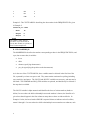
Example 1: A CULTIVARS file describing the observations of the FREQUENCES file.
statut
nom_var
echant Å Name of the variables in file head
r
L1
1
r
L2
1
r
L3
1
r
L4
1
r
L5
1
r
L3
1
r
L7
1
3
r
L8
1
r
L9
1
r
L10
1
Example 2: The CULTIVARS file describing the observations in the FREQUENCES file given
in Example 2.
Statut nom_var echant
.
Barlet
10
.
Barpolo
8
.
Barylou
6
The variable “statut” must be
specified. If you do not wish to
specify this variable, use periods, as
shown in the example here.
B. 2 The MARKERS file
The MARKERS file describes the markers corresponding to those in the FREQUENCES file, and
up to, but no more than, 4 variables:
•
locus
•
allele
•
chromo (specifying chromosome)
•
pos_chr (specifying the position on the chromosome)
As in the case of the CULTIVARS file, these variables must be declared in the first line of the
file, separated by at least one space or tab. They must remain consistent for spelling (including
case sensitivity) and spaces. The LOCUS and ALLELE variables are necessary, and must not be
left blank. The CHROMO and POS_CHR variables are optional, and should only be declared if
the map data is available.
The LOCUS variable is alpha-numeric and identifies the locus of various markers (bands or
alleles). In cases where the allele relationship between the markers is known, the identifier of a
given locus should appear in the first column as many times as there are indexed alleles. In
Example 1 below, the locus header ADH2-H is repeated 8 times to indicate each of its alleles,
named 1 through 8. In cases where the allelic relationships between markers are unknown, each
4
individual marker is identified by the locus variable, as if it were a separate locus (see Example 2
below).
The variable ALLELE identifies the alleles at each locus, by a number, a letter or by molecular
weight (see Example 2). The variable CHROMO is a numeric variable used to identify the
linkage group or chromosome of the analyzed locus. The variable POS_CHR is also numeric,
and indicates the position of the locus on the linkage group or chromosome in centimorgans,
compared to neighboring loci.
Note: The data must be separated by at least one space or tab.
Example 1: A MARKERS file describing the columns indicated in the FREQUENCES file given
in Example 1 above, and assuming co-dominant loci with defined alleles.
Known map position
locus allele chromo pos_chr ÅName of the variables in file head
ADH2-H 1 4 9.7
ADH2-H 2 4 9.7
ADH2-H 3 4 9.7
ADH2-H 4 4 9.7
ADH2-H 5 4 9.7
ADH2-H 6 4 9.7
ADH2-H 7 4 9.7
ADH2-H 8 4 9.7
C10-H B 3 54.3
C10-H C 3 54.3
C10-H A 3 54.3
C102-E 1 3 61.4
C102-E 2 3 61.4
C102-E 3 3 61.4
C102-E 4 3 61.4
C102-E 5 3 61.4
5
Unknown map position
locus allele Å Name of the variables in file head
ADH2-H
1
ADH2-H
2
ADH2-H
3
ADH2-H
4
ADH2-H
5
ADH2-H
6
ADH2-H
7
ADH2-H
8
C10-H
B
C10-H
C
C10-H
A
C102-E
1
C102-E
2
C102-E
3
C102-E
4
C102-E
5
Example 2: A MARKERS file describing the columns indicated in the FREQUENCES file given
in Example 2, above, and assuming dominant loci (i.e., allelic relationships between bands do not
exist or are not known).
locus
allele
Gen01
72
Gen02
77
Gen03
83
Gen04
91
Gen05
10
Gen06
108
Bar29
277
Bar30
280
Bar31
284
Bar32
289
6
AFLP Marker name
Molecular weight of the bands
B. 3 The FREQUENCES file
The FREQUENCY file contains as many observations (lines) as there are individuals (OTUs)
analyzed to characterize a population, as described in the CULTIVARS file. This value will be
one, if it is a pure line cultivar or single cross hybrid. It also contains as many variables
(columns) as the number of markers (described in the MARKERS file) characterizing these
OTUs. Each line corresponds to the frequency profile of the markers of each given individual.
Notice that these frequencies are discrete: 0, 0.5 or 1 in each diploid individual; 0, 0.25, 0.5, 0.75
or 1 in each tetraploid individual, etc. for higher ploidy levels.
Note: The data must be separated by a space or a tab, and missing data indicated by a period (.).
The first record should start on the second line, and the first line is reserved for a description of
the file (origin and type of data), written as a SAS comment, that is, beginning with the /*
symbols
and ending with the */ symbols
Example 1: FREQUENCES file of 10 homogenous varieties (10 pure line OTUs) characterized
by 3 loci having 8, 3 and 5 alleles each (with a total of 16 variables). Note that the frequencies of
the alleles at each locus within an individual must sum to 1. Because these are pure lines, only
homozygous states (0 or 1) are recorded in this example.
Example 2: FREQUENCES file for 3 heterogeneous varieties characterized by 10 AFLP
markers; numbers of individuals (lines) per population were defined in the CULTIVARS file
showed in example 2.
7
--Line reserved for comments1
1
1
0
1
1
1
1
0
1
1
1
1
0
1
1
1
1
0
1
1
1
1
1
1
1
1
1
0
1
1
0
1
0
1
1
1
1
0
1
1
1
1
0
1
1
1
1
0
1
1
0
1
0
1
1
1
1
0
1
0
1
1
0
1
1
1
1
1
1
1
1
1
1
0
1
1
1
0
1
1
1
1
1
1
1
1
1
0
1
1
1
1
1
1
1
1
1
1
1
1
1
1
0
1
1
1
1
0
1
1
1
1
1
1
1
1
1
0
1
1
1
1
0
1
0
1
1
0
1
0
1
1
0
1
1
1
1
0
1
1
1
1
0
1
1
1
1
0
0
1
1
1
0
1
1
1
1
0
1
0
1
1
0
1
1
1
1
0
1
1
1
1
0
1
1
1
1
1
0
1
1
0
1
1
1
1
1
1
1
1
1
1
1
1
1
1
1
1
1
1
1
1
0
1
1
0
1
1
1
1
1
0
0
1
1
1
1
0
1
1
1
1
0
1
1
1
1
0
1
1
1
1
0
1
1
1
1
1
1
Variety 1 (10 indivuals)
C. Analyses performed by the program
C.1 Genetic diversity measurements
Regardless of the type of OTU, the program estimates:
1. in the case that the molecular information can be classified as <<locus-allele>>
•
The number of alleles per locus in this study
•
Nei’s diversity index for populations in panmixis over all loci in the study.
Al
( )
H = 1 − ∑ Pˆal
l
e
8
a =1
2
(Nei, 1973),
Variety 2 (8 individuals)
Variety 3 (6 individuals)
The data is separated
by tabs.
Where Al equals the total number of alleles for locus l, and P̂al , the estimated frequency of allele
a at locus l in the current study.
2. in the case that molecular information can be classified as « bands »,
•
The frequency of the markers (bands) in the study.
•
The PIC (Polymorphism Information Content) of the markers, which is equivalent to Nei
diversity estimate for biallelic loci:
PIC = 2 pˆ m (1 − pˆ m ) ,
Where P̂m is the estimated frequency of the marker m in the study.
If the collection is composed of heterogeneous varieties, the program estimates:
•
The average number of individuals characterized by locus and by variety.
•
The mean number of alleles within each variety over all loci in the study.
•
The Nei diversity index (markers « locus-alleles ») or PIC value (markers « bands »)
within each variety in the study:
( )  (Nei, 1978),
Al
1 L  2nl 
1 − ∑ Pˆali
H = ∑
L l =1  2nl − 1  a =1
i
e
2

Where L is the total number of loci characterized for variety i, nl is the number of individuals
characterized for locus l, and P̂al is the estimated frequency of allele a at locus l for variety i.
C.2 Principal Components Analyses (PCA)
1. Homogenous Varieties:
The program will perform a PCA on the matrix of genetic distances calculated from the
frequencies of the markers (alleles or bands) stored in the FREQUENCES file. Missing data is
replaced by the frequency of the markers within all varieties in the study .
The quality of the graphical representation of an OTU is estimated by the square of the cosine of
the angle θ between the original vector in the space represented by the centered and reduced
9
variables (bands or alleles) and its projection on the principal axis (under 2 spatial dimensions).
This approaches one as the area between the 2 vectors becomes very small ( Cos 2θ → 1 when
θ → 0 ). It is graphically symbolized by a circle (centered on the variety).
2. Heterogenous Varieties:
The program performs two different Principal Components Analyses for heterogeneous varieties:
▪
A PCA on the correlation matrix of the frequencies of the markers (alleles or bands)
estimated within each population. The graphical output is calculated and represented as in
C.2.1, homogenous varieties.
▪
A PCA on the correlation matrix of the frequencies of the markers with the individuals of
each population analyzed separately (individual data of the FREQUENCES file). The
missing data are estimated as in C.2.1. The Euclidian center of the cloud of points formed by
the individuals in each population is calculated, and represented in a graphic with together all
of the individual points.
C.3 Estimation of the genetic distances and precision of the estimates
1. Homogenous variety – «locus-allele» markers:
Squared Modified Rogers (1972) distance estimator is used by the program:
D Rij =
(
1 L Al i
Pal − Palj
∑∑
2 L l =1 a =1
)
2
,
Where L is the total number of loci characterizing the i and j varieties being compared; Al,, is the
number of observed alleles at locus l in the collection; and Pali ( Palj ), the frequency of allele a
of locus l in the variety I (j). In the case where i and j are pure lines, the Squared Modified
Rogers distance estimates the percentage of the loci for which the lines differ.
The sampling variance of the Squared Modified Rogers distance is estimated by:
Var ( DRij ) =
▪
DRij (1 − DRij )
L
(Dillmann, 1997).
If the collection of OTUs is made up of simple hybrids, or the varieties are incompletely fixed
lines (ie, residual heterozygosity for at least one locus in at least one line) the approximate
10
boundaries of the Squared Modified Rogers distance confidence intervals are estimated by
assuming a normal distribution of the distance:
Inf ( DRij ) = DRij − uα Var ( DRij ) , and
Sup ( DRij ) = DRij + uα Var ( DRij ) ,
with uα , the Z-value by the normal standard table for a chosen probability level α.
▪
If the collection of OTUs to be analyzed is solely made up of pure line varieties (ie,
homozygous for all the loci in all the lines), and if we assume that the loci are independent
and unlinked, the Rogers distribution follows the binomal distribution B ( L, DRij ) . In this
case, the exact boundaries of the Squared Modified Rogers distance confidence interval is
calculated according to Collett, (1991) :
Inf ( DRij ) =
Sup ( DRij ) =
▪
[(
LD Rij + L 1 − DRij
LD Rij
, and
+ 1 F(1−α / 2) [2[L (1− D ij ) +1]; 2 LD ij ]
) ]
R
R
LD Rij + 1
LD Rij + 1 + L 1 − DRij F(α / 2 )[2 L (1− D ij ); 2( LD ij +1) ]
(
) (
)
R
R
If the varieties are pure lines, and the CHROMO and POS_CHR variables of the MARKERS
file have been given for at least a part of the locus (Cf. B.3), the program estimates in
addition to the Squared Modified Rogers distance, the BLUE (Best Linear Unbiaised
Estimator) of the Squared Modified Rogers distance (Dillmann et al. 1997) estimated from
the mapped loci:
(
)
−1
~
DBij = 1'V −11 (1'V −1 ) DRij
Where 1 is the dimension identity of the vector (L*,1) ; DRij (={0,1}),the Squared Modified
Rogers distance vector estimated for L* individual locus between the i and j varieties; and V is the
variance-covariance of the Squared Modified Rogers distance for the individual locus, estimated
by the map distance between locus.
11
~
The D Bij variance is estimated by:
−1
~
Var ( DBij ) = (1'V −11) .
The approximate boundaries of the confidence intervals of the Squared Modified Rogers
~
distances observed are estimated under the normality hypothesis of D Bij :
~
~
~
Inf ( DBij ) = DBij − uα Var ( DBij ) and,
~
~
~
Sup ( DBij ) = DBij + uα Var ( DBij )
2. Homogenous variety – «band» markers:
This distance estimator used in this case is that of Nei and Li (1979):
DNij = 1 −
2 N ij
,
Ni + N j
Where Nij is the number of common bands between varieties i and j; and Ni (Nj), the number of
bands for the variety i (j). For information only, the distance of Jaccard (1900; 1908) is deducted
from the distance of Nei&Li:
DJij =
2 DNij
(Snijders et al., 1990)
1 + DNij
The variance of the Nei and Li distance is estimated by:
(
)
 N ij 1 − 2 N ij / m v( N ij ) 2 
Var ( DNij ) ≈ 4 
+
 , (Dillmann, 1999; pers. com.)
m2
m4 

Where m is the average and v is the variance of the total number of bands present within every
pair of varieties within the study.
m=
v=
nV nV
2
(
N i + N j ) , and
∑∑
nV (nV − 1) i =1 j >i
(
nV nV
2
Ni + N j
∑∑
nV (nV − 1) i =1 j >i
)
2
− m2
Where nV equals the number of varieties in the study.
12
This estimate assumes that N ij follows a binomial distribution with N and P calculated as:
N=
E( N i + N j ) m
N ij 2 N ij
≈ , and P =
≈
2
2
N
m
The approximate confidence interval of the Nei and Li distance is estimated as:
Inf ( DNij ) = DNij − uα Var ( DNij ) , and Sup ( DNij ) = DNij + uα Var ( DNij ) .
If requested by the user, the program will estimate the confidence interval using the values
observed following repeated sampling with replacement (the bootstrap procedure). This method
is recommended, as the analytical estimation can become very imprecise for small sample sizes.
3. Heterogenous varieties – «locus-allele» markers:
Two types of distances can be used by the program: Squared Modified Rogers distance (1972)
and Sanghvi (Foulley and Hill, 1999).
The Squared Modified Rogers distance estimate is calculated by:
(
1 L Al ˆ i ˆ j
~
DRij =
∑∑ Pal − Pal
2 L l =1 a =1
ˆi ˆi
ˆj ˆj
) − 21L ∑∑  PN P− 1 + NP P− 1  ,
L
2
Al
l =1 a =1
a '> a

al a 'l
i
al a 'l
j

Where L is equal to the number of loci characterizing the varieties i and j, P̂ali ( P̂alj ), is the
estimated frequency of allele a at the locus l in the variety i (j), and Ni (Nj) is the number of
individuals in the variety i (j).
The confidence interval is estimated using the values observed following repeated sampling with
replacement (the bootstrap procedure). To remove bias from the estimation of the distance which
can occur in this resampling of individuals within varieties, the distance is recalculated as:
(
1 L Al ˆ i* ˆ j*
~**
DRi j =
∑∑ Pal − Pal
2 L l =1 a =1
)
2
*
*
*
*
1 L Al  Pˆali Pˆai'l Pˆalj Pˆaj'l Pˆali Pˆai'l Pˆalj Pˆaj'l 
,
−
+
+
+
∑∑
2 L l =1 a =1  N i − 1 N j − 1 N i − 1 N j − 1 
a '> a
*
*
Where Pˆali ( Pˆalj ) is the estimated frequency allele a has at the locus l in the bootstrap values
of i* (j*) for the variety i (j).
13
The Sanghvi distance estimate is calculated by:
Dˆ Sij =
(
L Al
Pˆali − Pˆalj
1
∑∑ Pˆ
A+ − L l =1 a =1
al
)
2
,
Where A+ is equal to the total number of alleles on the sample of the L loci analyzed, and P̂al ,
the estimated frequency of allele a at the locus l in the variety sampled.
The variance of the Sanghvi distance estimate is calculated according to Foulley and Hill (1999):
Var ( DSij ) =
1
( A+ − L )2
∑ 2( A − 1)(Dˆ
L
l =1
l
ijl
S
)
2
+ 1/ N ,
Where D̂Sijl is the estimated Sanghvi distance for locus l between the varieties i and j, and N is the
harmonic average of the number of individuals in the varieties i and j. N is calculated by :
N=
1
1 
 1
2 i + j 
N 
N
.
4. Heterogenous varieties – «band» markers:
These distances are calculated using Rogers (1972) calculation, which estimates distance as:
1
~
DRij =
M
∑(
M
m =1
Pˆmi − Pˆmj
)
2
1
−
M
(
)
(
)
 Pˆmi 1 − Pˆmi
Pˆmj 1 − Pˆmj 
+

 (Ghérardi and al., 1998),
∑
N i −1
N j −1 
m =1 
M
Where M is equal to the total number of markers (bands), P̂mi ( P̂mj ) is the estimated frequency of
the marker m within the variety i (j), and Ni (Nj) is the number of individuals in the variety i (j).
Note: this distance is estimated under the hypothesis that every marker (band) is a dominant allele
of a biallelic locus. This hypothesis is acceptable in the case of dominant marker types, such as
RAPD or AFLP. Use of this distance estimator will be incorrect in the cases of codominant
markers scored merely as present or absent, because knowledge of the genetic relationships
among alleles will be missing from the program. In these cases, the Squared Modified Rogers
distance calculated here will overestimate the distance between varieties.
The confidence interval is estimated using the values observed following repeated sampling with
replacement (the bootstrap procedure). To remove bias from the estimation of the distance that
can occur in this resampling of individuals within varieties, the distance is recalculated as:
14
~** 1
DRi j =
M
∑ (Pˆ
M
m =1
i*
m
− Pˆ
j*
m
)
2
1
−
M
(
)
(
)
(
)
(
ˆ j 1 − Pˆ j Pˆ i* 1 − Pˆ i* Pˆ j* 1 − Pˆ j*
 Pˆmi 1 − Pˆmi
P

+ m j m + m i m + m j m
∑
i

N −1
N −1
N −1
N −1
m =1 
M
) ,


Where M is equal to the total number of markers, P̂mi ( P̂mj ) is the estimated frequency of the
marker m in the initial sample of the variety i(j), and P̂mi ( Pˆmj ), the frequency of the marker m in
*
*
the resampling of the variety i (j).
C.4. Hierarchical Classification
To visualize the results of the distances in the matrices, the program will perform a hierarchical
classification, using four different methods for the user to choose from. Details of the methods
can be found in Bouroche and Saporta, (1980). Formulas to calculate the distances between
groups formed in the preceding steps and any given element k using the following four methods:
•
UPGMA (Unweighted Pair Group Average Method)
d [k , (i ∪ j )] = pi d (i, k ) + p j d ( j , k ) ,
where
pi = ni /(ni + n j ) (weights assigned to group i) and,
p j = n j /(ni + n j ) (weights assigned to group j).
•
Ward (minimum variance within groups)
d [k , (i ∪ j )] = ( pk + pi )d (k , i ) + ( pk + p j )d (k , j ) − pk d (i, j ) ,
where
pk = nk /(nk + ni + n j ) (weights assigned to group k),
pi = ni /(nk + ni + n j ) (weights assigned to group i), and
p j = n j /(nk + ni + n j ) (weights assigned to group j).
•
Minimum (nearest neighbor)
d [k , (i ∪ j )] = min[d (k , i ), d (k , j )]
•
Maximum (furthest neighbor)
d [k , (i ∪ j )] = max[d (k , i ), d (k , j )]
If the user requests it, a bootstrap procedure will be used by the program to test the stability of the
junctions in the original dendrogram. The stability of these junctions or join points is estimated
by the percentage of times where the varieties joined by this junction in the original dendrogram
are grouped together in the dendrograms calculated by each resample during the bootstrap
procedure:
15
Rdc =
(100 N dc* )
N d*
’
Where Rdc is the stability of the junction c in the original dendrogram d, N dc* is the number of
times where junction c is preserved among the trees produced in each resample, and N d * is the
total number of resampling done in the bootstrap.
Note: the calculations of stability of the junctions are considered only for dendrograms
constructed using Rogers and Nei and Li distances.
D. Installation of LCDMV and practice session
To use LCDMV, you must have a recent version of SAS (later than version 6.10) running on a PC
or Unix, installed with the IML (Interactive Matrix Language). The complete LCDMV software
package contains:
1. A catalog of macros called Sasmacro.Sc2
2. A catalog of devices called Devices.Sc2
3. A permanent SAS file called Varstore.Sd2
4. A SAS program called Lcdmv.sas
These four elements are required, and must be stored in the same folder (for example,
c:\logiciel\Lcdmv). When these elements have been copied to the folder of your choice, you
must open the program Lcdmv.sas (menu Spins-orders Open) in interactive method (the windows
PROGRAM EDITOR, OUTPUT, and LOG must be accessible) as below, and replace MONREP
by the name of the path and folder under which you have saved the four elements of the LCDMV
program (formerly : C: \logiciel\Lcdmv).
Note: Modifying any other part of this file could result in errors or loss of function.
16
In order to use the C:\logiciel\lcdmv path as the default path you must do the next changes:
/*---------------------PROGRAMME LCDMV---------------------*/
/*++++++++++++++++++++++++++++++++++++++++++*/
options nosource Mstored sasmstore=logiciel;
Libname logiciel 'C:\logiciel\lcdmv';';
Libname logiciel 'C:\logiciel\lcdmv';
%global DdisP DdisL DimpP DimpL;
%let DdisP=WINdisP; %let DdisL=WINdisL;
%let DimpP=CLJPSA4P;
%let DimpL=CLJPSA4L;
17
%Prog_P;
/*++++++++++++++++++++++++++++++++++++++++++*/
Save the modification that you have made (menu Spins – orders Knows; or by clicking the save
button) and run the program with the Submit command from the Local menu or by clicking the
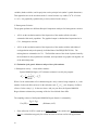
following icon:
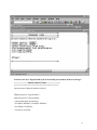
When the program has finished running successfully, you should see the FILES window appear
within a few seconds:
Indicate the following:
1.
The complete path under which you saved the three files necessary to run the
software (for example: C: \logiciel\lcdmv\files\maïs\RAPD),
2.
the name of the 3 entry files (for example, V_rapd. dat, M_rapd. dat, and
P_rapd.dat),
3.
The complete path under which you wish the resulting files to be stored (for
example: C:\logiciel\lcdmv\results\maïs\RAPD), and
4.
the prefix that you wish to give the results file, to distinguish them from the input file
(for example, RAPD).
18
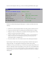
Upon successful completion of this step, you will see the following OPTIONS window appear:
You then can validate the data using the default options or continue to modify the data by the
following:
•
Perform a PCA, while specifying the number of axes that you wish to examine (up to five ).
•
Change the classification method to something other that UPGMA (Ward, for example).
•
Display the varieties on a different scale, for example to show them grouped more closely
together by specifying a larger distance threshold.
•
Calculate a confidence interval on the genetic distance estimates, or test the robustness or
stability of the join points of the dendrogram by performing a bootstrap analysis and
specifying the number of resampling to use.
•
Choose the confidence level of the confidence interval of the estimated genetic distances.
Upon choosing one of these analysis options, the program begins calculations and progressive
editing of the output. The output graphic will depend on the analysis chosen, and the
combination of variety type and marker type, as identified by the program and specified by your
input files. During the execution of the program, you may wish to move to the GRAPH window
to see the output. If you wish to examine in detail or to modify an output graph (for example, to
change the legend), you can use the command Edit Graph from the Edit menu or by clicking on
following icon:
19
The End command of the Spins menu (graphic editor) allows you to return to the GRAPH
window. You then can decide to print the graph or to save it to a file. To do so, go to the Spins
menu and chose the Print command. Export the file to be printed; by default, the graphs are in a
postscript (.ps) format. Only printed postscript copies can guarantee you the same format; using
other options may give random results and you will need to check the settings on your printer.
However, by Exporting the file, you will have different options for saving the graphics.
To verify the results of the analyses performed by the program, check the file created by the
program (it will be named “prefix.out” where prefix is the name of your input file). You will find
3 to 4 text files corresponding to the files specifying variety type of the cultivars analyzed and the
type of marker used. The prefix you use in naming the files is followed by a number in order of
their creation; ie, RAPD_1, RAPD_2, …).
Without exiting the SAS program, you can recall the program Lcdmv.sas (Local menu – Recall
text command) which will place you in the PROGRAM EDITOR window. This will relaunch the
execution of the program. Because files are edited progressively as you work and saved
sequentially in the folder WORK.GSEG that already contains the graphs created in the first
session, you will soon have many files in this folder. However, these files are automatically
destroyed the moment you exit the SAS program. You must remember to print or save the graphs
you wish to keep using the Print or Export commands from the Spins menu.
20
F. References
Bouroche JM et G Saporta (1980) L’analyse des données. Que sais-je. PUF.
Collet D (1991) Modeling binary data. London : Chapman & Hall, pp. 23-25.
Dillmann C., A. Charcosset, B. Goffinet, JSC Smith et Y. Dattée (1997) Best linear unbiased
estimator of the molecular genetic distance between inbred lines. Advances in Biometrical
Genetics. Proceedings of the Tenth Meeting of EUCARPIA Section Biometrics in plant
Breeding, Posnań, 14-16 May 1997, P. Krajewski and Z. Kaczmarek (eds.), pp. 105-110.
Foulley JL et WG Hill (1999)A propos de l’estimation de la précision d’estimation de la distance
génétique. XXXI Journées de Statistiques. 17-21 Mai 1999, Grenoble. Session Biométrie et
Génome.
Ghérardi M, B Mangin, B Goffinet, D Bonnet, T Huguet (1998) A method to measure genetic
distance between allogamous populations of alfalfa (Medicago sativa) using RAPD
markers. Theor. Appl. Genet. 96 :406-412.
Jaccard P (1900) Contribution au problème de l’immigration post-glaciaire de la flore alpine.
Bulletin de la Société Vaudoise des Sciences Naturelles 37 :547-579.
Jaccard P (1908) Nouvelles recherches sur la distribution florale. Bulletin de la Société Vaudoise
des Sciences Naturelles 44 :223-270.
Nei M (1973) Analysis of gene diversity in subdivided populations. Proc Natl Acad Sci USA
70 :3321-3323.
Nei M (1978) Estimation of average heterozygosity and genetic distance from a small number of
individuals. Genetics 89 :583-590.
Nei M et WH Li (1979) Mathematical model for studying genetic variation in terms of restriction
endonucleases. Proc Natl Acad Sci USA 76 :3269-3273.
Rogers JS (1972) Measures of similarities and genetic distances. Studies in genetics VII. Univ
Texas Publ 7213 :145-153.
Snijders TAB, M Dormaar, WH van Schuur, C Dijkman-Caes et G Driessen (1990) Distribution
of some similarity coefficients for dyadic binary data in the case of associated attributes. J
Clas 7 :5-31.
21
P. Dubreuil, C. Dillmann,
M. Warburton, J. Crossa,
J. Franco and C. Baril
April 2003
First Edition
Apdo. Postal 6-641, CP 06600. Mexico D.F, MEXICO
www.cimmyt.org