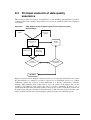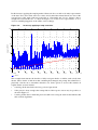
1
Good Practice Guide for Air Quality
Monitoring and Data Management 2009
This report may be cited as:
Ministry for the Environment. 2009. Good Practice Guide for Air Quality Monitoring and
Data Management 2009. Wellington: Ministry for the Environment.
Published in April 2009 by the
Ministry for the Environment
Manatū Mō Te Taiao
PO Box 10362, Wellington 6143, New Zealand
ISBN: 978-0-478-33166-0 (print)
978-0-478-33167-7(electronic)
Publication number: ME 933
© Crown copyright New Zealand 2009
This document is available on the Ministry for the Environment’s website:
www.mfe.govt.nz
Acknowledgements
The Ministry would like to thank the following people and organisations for contributing to the
development of this guide:
•
Clean Air Society of Australia and New Zealand, represented by Paul Baynham
•
National Air Quality Working Group members
•
National Institute of Water and Atmospheric Research Limited
•
regional council air quality scientists
•
the practitioners who attended a consultation workshop in December 2008:
− Teresa Aberkane, Environment Canterbury
− Robert Chauval, QEMS Ltd
− Brian Cheyne, Taranaki Regional Council
− Ross Glubb, Environment Canterbury
− Sally Gray, National Institute of Water and Atmospheric Research Limited (NIWA)
− Shane Iremonger, Environment Bay of Plenty
− Nick Kim, Environment Waikato
− Brian Mills, BECA
− Deborah Mills, Otago Regional Council
− Tamsin Mitchell, Greater Wellington Regional Council
− Janet Petersen, Auckland Regional Council
− Jozua Taljaard, Watercare Services Ltd.
Good Practice Guide for Air Quality Monitoring and Data Management 2009
iii
Abbreviations
µg/m³
micrograms per cubic metre
µm
micrometre
AAQG
Ambient Air Quality Guidelines
AS/NZS
Australian / New Zealand Standard
BAM
beta attenuation monitor
BaP
benzo(a)pyrene
BS EN
British Standards Institution European Norm standard
CFR
United States Code of Federal Regulations (40 CFR 51 is the same as Title 40, Part 51 of the
CFR)
CO
carbon monoxide
DAS
data acquisition system/datalogger
FDMS
filter dynamics measurement system
H2S
hydrogen sulphide
Hi-vol
high-volume sampler
mg/m³
milligrams per cubic metre
NAQWG
National Air Quality Working Group
NES
national environmental standards
NIWA
National Institute of Water and Atmospheric Research Limited
NMHC
non-methane hydrocarbon
NO
nitric oxide
NO2
nitrogen dioxide
NOx
oxides of nitrogen (eg, nitrogen dioxide and nitrous oxide)
NZST
New Zealand Standard Time
O3
ozone
PAH
polycyclic aromatic hydrocarbon
PM2.5
particulate matter with an aerodynamic diameter of 2.5 microns or less
PM10
particulate matter with an aerodynamic diameter of 10 microns or less
PMT
photomultiplier tube
ppb
parts per billion
ppm
parts per million
RMA
Resource Management Act 1991
SO2
sulphur dioxide
TEOM
tapered element oscillating microbalance
TSP
total suspended particulate
USEPA
United States Environmental Protection Agency
UV
ultraviolet
VOC
volatile organic compounds
WHO
World Health Organization
iv
Good Practice Guide for Air Quality Monitoring and Data Management 2009
Contents
Acknowledgements
iii
Abbreviations
iv
1
Introduction
1
1.1
1.2
1.3
1.4
1.5
1.6
1
1
2
3
3
4
2
3
Why Monitor? – Monitoring Programme Objectives
6
2.1
2.2
2.3
2.4
2.5
6
6
7
8
9
Monitoring for standards and guidelines
Meteorological monitoring
How to Monitor? – Monitoring Methods
4.1
4.2
4.3
4.4
4.5
4.6
4.7
4.8
4.9
5
Regional policies and plans
Regional monitoring objectives
Developing an air quality monitoring programme
Desktop assessments
Types of monitoring
What to Monitor? – Choosing Contaminants
3.1
3.2
4
Purpose of the Guide
Background
Who will use this Guide?
Status of recommendations
What this Guide covers
What this Guide doesn’t cover
Using appropriate monitoring methods
Using existing monitoring for national environmental standards
Choosing appropriate monitoring equipment
Methodology types
Mandatory ambient air monitoring methods
Recommended ambient air monitoring methods
Open-path monitoring systems
Meteorological monitoring
Monitoring agencies and training
Particulate Monitoring
5.1
5.2
Monitoring for different fractions
Methods for particulate monitoring
Good Practice Guide for Air Quality Monitoring and Data Management 2009
11
11
14
15
15
16
17
18
19
22
25
25
26
28
28
30
v
6
Where to Monitor? – Selecting Monitoring Sites
6.1
6.2
6.3
6.4
6.5
6.6
7
The Australian / New Zealand Siting Standard
Site classification
Considerations for site selection
Representativeness of monitoring sites
Further monitoring considerations
Long-term viability of sites
Equipment Calibration and Maintenance
7.1
7.2
7.3
7.4
7.5
7.6
8
Overview
Equipment calibration
Equipment maintenance
Procedures and documentation
Training
Recommended equipment calibration methods for NES for air quality
contaminant monitoring
Data Management Protocols
8.1
8.2
8.3
8.4
8.5
8.6
8.7
8.8
8.9
8.10
9
Data quality assurance
Documentation and procedures
Principal elements of data quality assurance
Data adjustment
Data validation
Negative data
Missing data
Monitoring site metadata
Monitoring units
Conversion factors
Reporting Monitoring Results
9.1
9.2
9.3
9.4
Time formats
Reporting data formats
Significant digits and rounding protocols
Summary statistics
References
vi
Good Practice Guide for Air Quality Monitoring and Data Management 2009
35
35
35
36
38
39
41
42
42
42
48
49
51
52
56
56
58
59
61
66
67
68
69
71
72
75
75
75
76
77
79
Appendices
Appendix A: Time Averages (NES for Air Quality, Schedule 1)
Appendix B: Wind Speed Conversions and Presentation of Wind Speed Data
Appendix C: Sample Filter Characteristics and Applications
Appendix D: Particulate Monitoring Instruments Commonly Used in New Zealand
Appendix E: Examples of Routine Check-sheets for a BAM Instrument and a CO
Analyser
Appendix F: Example of a Maintenance and Calibration Record for an FH62
Instrument
Appendix G: Quick Reference Conversion Tables
Appendix H: Summary of Recommendations
81
82
83
84
85
88
91
92
Tables
Table 1:
National environmental standards for ambient air quality
12
Table 2:
Ambient air quality guidelines (2002)
13
Table 3:
New Zealand monitoring site classification and scales
36
Table 4:
Example of table showing PM10 summary statistics
77
Figures
Figure 1.1: Applications of the Ministry for the Environment’s air quality good practice
guides
5
Figure 7.1: Example of calibration results tracking for a CO analyser
45
Figure 8.1: Process elements that provide data quality assurance
57
Figure 8.2: Flow diagram of the acceptance process for routine air quality
measurements
59
Figure 8.3: Response curves used to calculate actual concentrations from recorded
instrument response R(x) at time T(x)
62
Figure 8.4: Example of baseline drift in CO data
63
Figure 8.5: Example of a sudden change in data baseline
63
Figure 8.6: Incorrectly applying a ramp correction
64
Figure 8.7: Extrapolating a calibration
65
Figure 9.1: Example of box plot showing contaminant distribution at different monitoring
sites
78
Figure 9.2: Example of figure showing the proportion of PM10 samples belonging to
different air quality categories
78
Good Practice Guide for Air Quality Monitoring and Data Management 2009
vii
1
Introduction
1.1
Purpose of the Guide
The Good Practice Guide for Air Quality Monitoring and Data Management 2009 provides
guidance to help achieve accurate and representative ambient air quality monitoring, using
nationally consistent monitoring methods and reporting formats. The Guide also aims to make
air quality monitoring information accessible by being a quick reference of methods and new
developments.
This document replaces the Good Practice Guide for Air Quality Monitoring and Data
Management published by the Ministry for the Environment in 2000. It does so by incorporating
the significant developments (see section 1.2) that have occurred since the 2000 Guide was
published.
This Guide aims to provide guidance for air quality monitoring and data management to ensure
these are:
•
correct – air quality monitoring is of high quality and free from errors
•
representative – spatial/temporal variations and the extent of human exposure are
considered when designing monitoring networks
•
consistent – air quality data is recorded, analysed, processed, reported and archived
following best-practice principles
•
accessible – suppliers and users of air quality data have quick and easy access to methods,
procedures and new developments.
1.2
Background
The Resource Management Act 1991 (RMA) requires regional councils / unitary authorities to
monitor air quality and the state of the environment. In response, councils have prepared
regional air quality plans, which contain objectives for air quality in the region together with
policies and rules to achieve them.
Historically, information on New Zealand’s air quality was limited to data from a small number
of monitoring sites. In recent years, many councils have designed and established air quality
monitoring programmes of varying scales and complexities, and since 1993 the number of air
quality monitoring sites in New Zealand has increased significantly (Ministry for the
Environment, 2003a).
As monitoring programmes were established and existing ones expanded, concerns have been
raised about data quality, reliability and comparability. In particular, data gathered by different
techniques or to varying levels of quality assurance prevented the development of a reliable
picture of air quality across New Zealand. To address these concerns, the Good Practice Guide
for Air Quality Monitoring and Data Management (2000) was developed by the Ministry for the
Environment in close collaboration with air quality specialists.
Good Practice Guide for Air Quality Monitoring and Data Management 2009
1
The objective of that guidance was to provide robust, good-quality monitoring and reporting
practices that would ensure:
•
the effectiveness of different air quality management options could be evaluated
•
the comparability of air quality data between sites and regions
•
clear communication of information about air quality and its effects within a region and
nationally (eg, through regional and national state of the environment reports).
Since the publication of the 2000 Guide there have been a number of developments.
•
Eight additional contaminants have been identified in the Ambient Air Quality Guidelines
(AAQG) (Ministry for the Environment, 2002), updating the original 1994 document.
•
New Zealand’s first suite of national environmental standards in the Resource Management
(National Environmental Standards Relating to Certain Air Pollutants, Dioxins and Other
Toxics) Regulations 2004 (the regulations) was introduced on 6 September 2004. The
regulations include the first ambient air quality standards in New Zealand, covering carbon
monoxide (CO), nitrogen dioxide (NO2), ozone (O3), particulate matter (PM10) and sulphur
dioxide (SO2).
•
The Foundation for Research Science and Technology (FRST) programme, Keeping Our
Air Clean, provided research and tools to help implement the national environmental
standards (NES) for air quality. Specific outputs from this programme have provided
additional guidance and resources for monitoring air quality, which are included in this new
Guide.
•
The national Air Quality Database, developed by the National Institute of Water and
Atmospheric Research Limited, was discontinued.
•
Annual, web-based national-level reporting of PM10 in monitored airsheds was introduced
in 2005. This includes data on concentration, methodology and exceedences, together with
straight-line-path information. This is a web-based update that can be accessed at the
Ministry for the Environment’s website
(www.mfe.govt.nz/state/reporting/air/nes/index.html).
These developments have led the Ministry to produce this updated guide, Good Practice Guide
for Air Quality Monitoring and Data Management 2009, to replace the 2000 Guide. The
Ministry intends to review and update the Guide as further developments occur (eg, the release
of new standards from Standards Australia and Standards New Zealand).
1.3
Who will use this Guide?
The Guide is primarily intended to be used by councils, agencies, consultants and researchers
when planning and carrying out:
•
regional air quality monitoring programmes
•
monitoring programmes to collect data for air quality models.
In addition, the Guide will be helpful for agencies planning and carrying out:
•
desktop assessments and screening surveys
•
various air quality research projects
•
other monitoring programmes.
2
Good Practice Guide for Air Quality Monitoring and Data Management 2009
1.4
Status of recommendations
The recommendations in this Guide represent best-practice approaches based on expert advice
from experienced air quality scientists in New Zealand. They should be used wherever possible.
However, the recommendations are not legislative requirements under the RMA or any other
legislation.
The recommendations should be closely followed when collecting monitoring data for
comparison with standards and guideline values or data from other locations. The methods are
consistent with those recommended for use in the NES for air quality and by Standards
Australia and Standards New Zealand. Different monitoring techniques may be useful when
monitoring for other purposes, such as screening surveys.
1.5
What this Guide covers
The Guide provides best-practice guidance for undertaking air quality monitoring for various
purposes. It also covers the statutory requirements for compliance monitoring and guidance for
monitoring other contaminants listed in the Ambient Air Quality Guidelines (AAQG). It deals
specifically with ambient air quality monitoring.
The Guide also covers the management of air quality data and includes guidelines for the
collection, review, storage and dissemination of such data.
Although the focus is on air quality contaminants, some discussion on meteorological
monitoring is included given that it plays a major role in the analysis and interpretation of air
quality monitoring data.
The Guide is structured as follows.
•
Chapter 1 (this chapter) describes the aims of the Guide and sets its scope. It provides
information on how the Guide was developed and explains the status of recommendations
contained in the Guide.
•
Chapter 2 contains guidance on developing an air quality monitoring programme and
discusses some types of monitoring.
•
Chapter 3 provides information on the contaminants included in the NES for air quality and
the AAQG and explains the difference between a standard and a guideline. It also briefly
discusses meteorological monitoring.
•
Chapter 4 discusses the different methodologies used in monitoring air quality. It lists the
required methods for compliance monitoring and the recommended methods for monitoring
AAQG contaminants.
•
Chapter 5 focuses on particulate monitoring. It describes the different particle size fractions
and the most common particle monitoring methods used in New Zealand.
•
Chapter 6 contains guidance on the siting of monitoring stations based on the latest
Australian / New Zealand standard (AS/NZS 3580.1.1:2007).
•
Chapter 7 discusses equipment calibration and maintenance procedures and provides
recommendations on proper documentation.
Good Practice Guide for Air Quality Monitoring and Data Management 2009
3
•
Chapter 8 contains guidance on data quality assurance at all stages of data management.
Guidance is also provided for data adjustment and dealing with negative and missing data.
•
Chapter 9 provides recommendations on data reporting formats to promote nationally
consistent air quality reporting.
1.6
What this Guide doesn’t cover
The Guide aims to provide information and recommendations that are neither too specific nor
too general. The scope of this Guide does not include:
•
equipment-specific guidance – readers are advised to consult the user’s manual or contact
the equipment vendor for detailed information
•
information on monitoring methods already covered by an Australian / New Zealand
Standard (AS/NZS), or other relevant standard – readers are advised to refer to the relevant
standard
•
emissions testing for individual source discharges – information about compliance
monitoring and emission testing can be found in the Ministry’s Compliance Monitoring and
Emissions Testing of Discharges to Air (1998)
•
monitoring odour – information on this can be found in the Ministry’s Good Practice Guide
for Assessing and Managing Odour in New Zealand (2003).
Figure 1.1 shows the full suite of the Ministry for the Environment’s air quality good practice
guide publications and their applications.
4
Good Practice Guide for Air Quality Monitoring and Data Management 2009
Figure 1.1:
Applications of the Ministry for the Environment’s air quality good
practice guides
Emission sources
Monitoring
Home
heating
Traffic
emissions1
3,
4
PM10
CO
NO2
O3
SO2
Air toxics
PM2.5
Dust5
Odour6
Visibility7
Industry2
Assessment
Emissions
inventory8
Monitoring
data3
Dispersion
modelling9
Natural
contribution
Photograph sources: Ministry for the Environment, Taranaki District Council and Tasman District Council
1
Good Practice Guide for Assessing Discharges to Air from Land Transport (2008)
2
Good Practice Guide for Assessing Discharges to Air from Industry (2008)
3
Good Practice Guide for Air Quality Monitoring and Data Management 2009 (2009)
4
Compliance Monitoring and Emission Testing of Discharges to Air (1998)
5
Good Practice Guide for Assessing and Managing the Environmental Effects of Dust Emissions (2001)
6
Good Practice Guide for Assessing and Managing Odour in New Zealand (2003)
7
Good Practice Guide for Monitoring and Management of Visibility in New Zealand (2001)
8
Good Practice Guide for Preparing Emissions Inventories (2001)
9
Good Practice Guide for Atmospheric Dispersion Modelling (2004)
Good Practice Guide for Air Quality Monitoring and Data Management 2009
5
2
Why Monitor? – Monitoring
Programme Objectives
The fundamental objective of air quality monitoring is to collect data that can be used to make
informed decisions to best manage and improve the environment. This section describes an
approach for developing an air quality monitoring strategy.
2.1
Regional policies and plans
Monitoring programmes should be closely linked to the main issues of concern within a region,
as specified in its regional plan. Air quality monitoring provides evidence on the current levels
of contaminants and provides policy-makers with information on how to better manage air
quality in their regions.
Air quality data is continuously collected to provide information to aid policy development and
evaluation. After a regional plan has been put in place, monitoring can confirm if targets are
being met and if the rules implemented are producing the anticipated results.
Compulsory monitoring requirements were also introduced when the NES for air quality were
implemented in 2004. Regional councils should consider these requirements when drafting their
regional plans and monitoring programmes.
2.2
Regional monitoring objectives
To quantify ambient air quality in a region and note spatial and temporal variations, the
monitoring should:
•
provide comprehensive data to judge the significance of actual and perceived regional
issues
•
be related to the issues, objectives and methods of implementation specified in the regional
air plan
•
supply sufficient data to determine geographical patterns in air quality over various time
scales (eg, seasonally)
•
lead to an understanding of whether national or regional air quality standards, guidelines,
objectives and environmental outcomes are being met, and whether areas of concern are
being identified
•
develop a picture of representative concentrations in areas of high population density where
air quality is known, or suspected, to be poor
•
provide sufficient data to determine trends in air quality over time and the background
levels of contaminants
•
supply enough information to determine the population at risk from exposure to poor air
quality in order to evaluate the potential and actual health effects in a region (eg, personal
exposure assessments).
6
Good Practice Guide for Air Quality Monitoring and Data Management 2009
2.3
Developing an air quality monitoring
programme
The intended use of data from a monitoring site should be identified before a site is established.
Usually, the general objective of an ambient air quality monitoring programme is to determine
air quality in a region to assess its effects on human health. However, programmes may have
different specific objectives (eg, to establish long-term trends and patterns, or validate
dispersion modelling).
There are many factors to consider in developing a monitoring programme, but the following
are of fundamental importance.
•
Why monitor?
Why is monitoring being undertaken? What is the expected outcome of the monitoring?
Establishing a monitoring objective is the fundamental step in developing a monitoring
programme because all subsequent decisions will be based on why the monitoring is being
undertaken. The most common reasons for monitoring include:
− determining the level of contaminants in an airshed to compare with standards and
guidelines
− reporting on the state of the environment
− obtaining exploratory data
− conducting air quality research
− obtaining data for air quality modelling
− providing air quality information for policy or strategy development
− assessing the effectiveness of policy based on air quality trends.
•
Which species to monitor?
In many cases this may be obvious, based on known emission sources in the area, but in
other cases it merits careful consideration. Once the target contaminant has been identified,
in what form should it be monitored? For example, total hydrocarbons or individual
(speciated) hydrocarbons? Total particulate matter or a specific size fraction? Is further
analysis required?
•
How to sample?
Both the type of sampling and the analytical end method need to be considered. Method
selection involves an appraisal of cost versus performance; the latter includes the limits of
detection, sensitivity, speed of instrument response, susceptibility to interfering species and
the overall uncertainty of the measurement. Consider the aim of monitoring and choose
appropriate methods and equipment. When using a screening method for exploratory
testing, is the level of accuracy and precision suitable to measure contaminant levels?
•
Where to sample?
The decisions around where to locate a monitoring site are based on the objectives of
monitoring. The siting of an air quality monitor has a profound effect on the resulting
measurements of contaminant levels and on achieving monitoring objectives. Will the site
measure peak or background concentrations? What atmospheric reactions affect the
formation/destruction of the contaminant to be monitored?
Good Practice Guide for Air Quality Monitoring and Data Management 2009
7
•
How to calibrate and maintain equipment?
Calibration and maintenance of monitoring equipment is an important part of every
monitoring programme. How frequently should calibration be undertaken? What
documentation is required? What procedures will ensure the efficient and smooth operation
of monitoring equipment?
•
What data management protocols should be used?
It is important to ensure that air quality data is properly validated and managed after it is
obtained. What data quality assurance processes are in place? What supplementary data
needs to be collected? Other information may be relevant to the study (eg, meteorological
conditions, process data and traffic flows). Meteorological conditions are important in
assessing the impacts of sources on surrounding areas because they dictate the transport and
dispersion of contaminants in ambient air.
•
How will data be stored and reported?
What time format should be used? How will exceedences be determined and reported?
Following the recommended format in the reporting of monitoring results is a step towards
achieving national consistency in air quality reporting.
These factors are discussed in greater detail in the following chapters.
2.4
Desktop assessments
In the early stages of establishing a regional monitoring programme little may be known about
the air quality of the area under investigation. Initially, it will be necessary to assess where air
quality in the region is likely to be at risk of exceeding standards for each contaminant. This can
often be done by a desktop assessment.
The following factors need to be investigated to determine areas at risk within a region:
•
emissions sources (eg, domestic, industrial, transport, agricultural and natural) and the
contaminants emitted
•
meteorology (eg, areas prone to temperature inversions)
•
topography
•
geography
•
population centres (especially where domestic fires and traffic emissions occur)
•
historical monitoring data (where available)
•
areas with high natural environmental values (eg, in and around natural parks, forests,
wilderness areas and wetlands)
•
the location of sensitive areas particularly vulnerable to air pollution (eg, hospitals, schools,
child- and aged-care facilities)
•
areas planned for development (eg, to get a picture of background concentrations)
•
any public complaints or issues of concern relating to air pollution
•
any epidemiological studies on air quality effects on health already carried out.
8
Good Practice Guide for Air Quality Monitoring and Data Management 2009
This information should provide a good basis to determine which contaminants should be
monitored and where contaminant levels may be elevated. Should any risks be identified,
preliminary screening surveys may need to be established to better identify risk areas and
potential contaminant levels, particularly if no historical monitoring data is available. Even with
a well-established regional monitoring programme, emission sources within an air quality
management area can change significantly over time (requiring an efficient approach to
updating emission inventories), and may result in the need for further screening surveys.
2.5
Types of monitoring
2.5.1
Screening surveys
Screening surveys using local knowledge and simple monitoring techniques can provide a quick
and cost-effective picture of contaminant concentrations over a wide spatial distribution. They
are usually intended to assess air quality at a particular location to determine indicative ambient
concentrations and identify whether more permanent monitoring is needed. Screening surveys
can include non-standard methods such as passive samplers for gases and volatile organic
compounds (VOCs) and low-volume gravimetric samplers for PM10. However, the use of
standard methods housed in a mobile air quality monitoring station may be more appropriate
where decisions on establishing permanent sites (at considerable financial investment)
are involved.
Consideration should be given to ensuring the monitoring period is representative of pollution
levels throughout the year. Screening should ideally be undertaken for at least a six-month
period to include summer and winter conditions. Screening surveys should cover particular
seasons in which contaminant peak levels occur.
2.5.2
Continuous monitoring
Screening programmes should only be used to provide an indication of where detailed
monitoring is required. Data derived from screening surveys must not be used to determine
whether an airshed complies with the NES for air quality or air quality guidelines. When there is
an indication that national standards are likely to be breached, it will be necessary to select sites
where contaminants will be monitored using the methods in Schedule 2 of the NES for air
quality. This is likely to require commitment to a long-term site in order to measure the effects
of management strategies in the airshed.
Two examples of continuous monitoring sites are:
•
permanent ambient site – a site established for long-term monitoring of contaminant levels
and trends using standard monitoring methods
•
compliance monitoring site – a site established for long-term monitoring of contaminant
levels and trends over time for the purposes of determining compliance with the NES for
air quality in a particular airshed. The use of standard monitoring methods is compulsory.
Good Practice Guide for Air Quality Monitoring and Data Management 2009
9
2.5.3
Monitoring for research purposes
Air quality monitoring is often undertaken for research purposes to address specific issues such
as local dispersion characteristics using tracer gases, or the collection of particle samples for
speciation analyses and source apportionment work. This work is usually carried out using nonstandard methods and specialised sampling equipment.
10
Good Practice Guide for Air Quality Monitoring and Data Management 2009
3
What to Monitor? – Choosing
Contaminants
This chapter describes the ambient air quality standards and guidelines and discusses how air
quality monitoring fits into the regulatory framework.
New Zealand has national environmental standards for five air contaminants as well as
15 ambient air quality guidelines. Guidelines that apply over the same averaging period for a
particular contaminant have been effectively superseded by the standards. This is not simply a
change in designation from guideline to standard. The following summarises the basic
differences between standards and guidelines.
•
Ambient air quality standards are concentration limits set to protect New Zealanders’
health. They have the force of regulation under the Resource Management Regulations
2004 and have mandated monitoring methods and reporting requirements. Some ambient
air quality standards incorporate a specified number of allowable exceedences in any
12-month period.
•
Ambient air quality guidelines are concentration limits recommended to protect human
health and the environment under the Resource Management Act 1991 (RMA). They may
be incorporated into regional plans as objectives or targets. The ambient air quality
guidelines do not specify allowable exceedences.
Note: Guidelines for contaminants not covered by standards still apply. Guidelines should be
followed as closely as possible for the sake of good practice and national consistency.
From a regulatory viewpoint, regional air quality plans are statutory instruments under the RMA
and have equal status with the standards. If the air quality objectives in a regional air quality
plan are more stringent than the NES for air quality, then the regional plan takes precedence.
Regional air quality objectives, however, cannot be more lenient than the NES for air quality
(Ministry for the Environment, 2008).
3.1
Monitoring for standards and guidelines
The term ‘airshed’ as used in the regulations is more akin to an ‘air quality management area’
rather than being a strictly science-based concept of an airshed (although in many instances the
two are equivalent). These airsheds were designated through recommendations made by
regional councils and unitary authorities to the Minister for the Environment. They extend
upwards from ground level, including coastal marine areas, and have no specified upper limit.
In most cases they represent areas that are known, or likely, to exceed the fine particle ambient
standard. The exception to this is the Marsden Point airshed, which is based on its likely or
known breaches of the sulphur dioxide standard.
Good Practice Guide for Air Quality Monitoring and Data Management 2009
11
3.1.1
National environmental standards (NES) for ambient air
quality
The NES for air quality apply at any place in the open air where a person might reasonably be
expected to be exposed to the contaminant over the relevant averaging period. This does not
include tunnels, indoor areas or outdoor workplace sites, whose emissions are covered by
Occupational Safety and Health regulations.
The standards are based on the ‘no observable adverse effect’ level or ‘lowest observable
adverse effect’ level in relation to human health. Where epidemiological studies and
international guidelines have been unable to determine such a threshold, a judgement has been
made as to what constitutes an ‘acceptable’ health risk.
Table 1 shows the airborne contaminants included in the NES for air quality which are
considered to be of greatest concern and most likely to exist in New Zealand.
Table 1:
National environmental standards for ambient air quality
Contaminant
Carbon monoxide (CO)
Threshold concentration
10 mg/m
3
Time average
Permissible excess per year
Running 8-hour mean
1
Nitrogen dioxide (NO2)
200 µg/m
3
1-hour mean
9
Ozone (O3)
150 µg/m
3
1-hour mean
0
50 µg/m
3
24-hour mean
1
3
1-hour mean
1-hour mean
9
0
PM10 (fine particles)
Sulphur dioxide (SO2)
350 µg/m
3
570 µg/m
The ambient standards came into effect on 1 September 2005. The standards include
permissible exceedences for CO, NO2, PM10 and the 350 µg/m3 SO2 standards. There are no
permitted exceedences for O3 or the 570 µg/m3 SO2 standards.
Certain human activities are associated with the emission of particular groups of contaminants.
Emissions from domestic fires monitored at a neighbourhood site may require the monitoring of
CO in addition to PM10. In areas where high sulphur content solid fuel is burnt, SO2 may be
another contaminant to monitor.
Refer to appendix A for Schedule 1 of the NES for air quality.
3.1.2
Ambient air quality guidelines
The Ambient Air Quality Guidelines (AAQG) are health-based guidelines that set the minimum
requirements that outdoor air quality should meet in order to protect human health and the
environment.
Table 2 outlines the existing 15 ambient air quality guidelines for a range of contaminants. This
includes guidelines with different values and time averages to the standards for carbon
monoxide (CO), nitrogen dioxide (NO2), ozone (O3), particulate matter (PM10), and sulphur
dioxide (SO2). These guidelines have not been superseded by standards because they measure a
different time average, and therefore provide an indication of human exposure on a different
time scale. It is important to assess air quality in terms of both short-term (eg, peak) exposure
and long-term exposure (eg, annual averages).
12
Good Practice Guide for Air Quality Monitoring and Data Management 2009
Table 2:
Ambient air quality guidelines (2002)
Contaminant
Guideline value
Carbon monoxide
30 mg/m
3
Nitrogen dioxide
100 µg/m
3
Ozone
100 µg/m
3
PM10
20 µg/m
Sulphur dioxide
b
Hydrogen sulphide
Lead
7 µg/m
d
Time average
1-hour mean
3
120 µg/m
c
a
24-hour mean
8-hour mean
Annual mean
3
24-hour mean
3
1-hour mean
0.2 µg/m
3
3-month rolling mean (calculated monthly)
3
Benzene (2002)
Benzene (2010)
10 µg/m
3
3.6 µg/m
Annual mean
Annual mean
1,3-butadiene
2.4 µg/m
3
Annual mean
Formaldehyde
100 µg/m
Acetaldehyde
30 µg/m
Benzo(a)pyrene
3
30-minute mean
3
Annual mean
0.0003 µg/m
d
3
Mercury (inorganic)
Mercury (organic)
d
0.33 µg/ m
3
0.13 µg/ m
Chromium IV
d
Chromium metal and chromium III
d
Arsenic (inorganic)
d
Arsine
3
Annual mean
Annual mean
Annual mean
0.0011 µg/m
3
0.11 µg/m
3
Annual mean
Annual mean
0.0055 µg/m
3
0.055 µg/m
3
Annual mean
Annual mean
Notes:
o
a
All values apply to the gas measured at standard conditions of temperature (0 C) and pressure (1 atmosphere).
b
The sulphur dioxide guideline values do not apply to sulphur acid mist.
c
The hydrogen sulphide value is based on odour nuisance and may be unsuitable for use in geothermal areas.
d
The guideline values for metals are for inhalation exposure only; they do not include exposure from other routes
such as ingestion. These other routes should be considered in assessments, where appropriate.
Monitoring PM2.5 is recommended if resources are available (see section 5, Particulate
Monitoring, for further details). Results may be compared with the World Health Organization’s
annual PM2.5 guideline of 10 µg/m3 (World Health Organization, 2006) or the monitoring
guideline of 25 µg/m3 (24-hour average) stated in the AAQG.
Additional guidance and information on the NES for air quality and the AAQG can also be
found in the following documents.
•
The Updated User’s Guide to Resource Management (National Environmental Standards
Relating to Certain Air Pollutants, Dioxins and Other Toxics) Regulations 2004 (Including
Amendments 2005) (Ministry for the Environment, 2005) is aimed at practitioners in local
government implementing the first suite of national environmental standards. Chapter 3 of
the User’s Guide deals with ambient air quality standards from an air quality management
and consent perspective.
•
Ambient Air Quality Guidelines (Ministry for the Environment, 2002) pre-dates the
introduction of the NES for air quality and includes guideline values for contaminants not
covered by the standards. Chapter 2 contains useful information on health effects and
sources of airborne contaminants. Although the NES for air quality has mandatory
considerations for the processing of resource consents, chapter 3 of the guidelines still
provides useful general guidance on regional air quality management.
Good Practice Guide for Air Quality Monitoring and Data Management 2009
13
3.2
Meteorological monitoring
Weather has a profound influence on contaminant dispersion and concentrations. For example,
meteorological effects such as temperature inversions can dramatically increase contaminant
levels. It would not be possible to gain a clear picture of the air quality in an area without
meteorological monitoring. Good-quality meteorological data is necessary, and may require a
number of stations depending on topography. Basic meteorological monitoring at some air
quality monitoring sites may prove very useful, especially when trying to assess the validity of
data. Meteorological data is also critical in the use of dispersion modelling.
A detailed set of guidelines for meteorological monitoring has been prepared by the United
States Environmental Protection Agency (USEPA, 2000). The Australian standard, AS
2923:1987, Measurement of horizontal wind, provides guidance on the measurement of wind
speed and direction. Additional guidance can also be sourced from the Guide to Meteorological
Instruments and Methods of Observation (World Meteorological Organization, 1996).
14
Good Practice Guide for Air Quality Monitoring and Data Management 2009
4
How to Monitor? – Monitoring
Methods
This chapter describes a range of methods for monitoring ambient air quality and outlines the
level of precision required for different monitoring purposes. Required methods for ambient air
quality standards and recommended methods for ambient air quality guidelines are discussed.
The chapter also includes a brief section on meteorological monitoring.
4.1
Using appropriate monitoring methods
A wide variety of methods are available for measuring contaminants in ambient air, with an
equally wide variation in cost and precision. Specific monitoring methods should be chosen
taking into consideration the purpose, objectives and budget of the monitoring programme.
Monitoring for the purposes of national environmental standards can only be carried out with
the high-precision instrumental methods in accordance with Schedule 2 of the regulations.
High-precision instrumental methods would also be generally used for research studies or other
specific investigations, where there is a need to understand the ways in which contaminant
levels fluctuate over short time periods (hours or days).
Ambient air quality guidelines carry recommended monitoring methods that should be used for
the assessment of the contaminants covered by the guidelines. These are based on Australian /
New Zealand and USEPA standards.
There is still a place for monitoring methods that fall outside the specifications for standards and
guideline assessments. Methods that involve lower resolution instruments can be used for an
initial screening survey, where a detailed study is not warranted. These may be used as a prelude
to more detailed monitoring. If contaminant levels are found to be low, then the same method(s)
could be used for repeat surveys over subsequent years. Low resolution methods are also useful
for prioritising a number of different areas that have already been selected for detailed
monitoring programmes.
It should be stressed that screening methods cannot be used to determine compliance with
national standards or guidelines. A screening method is any non-standard method that is used
on an exploratory basis and provides indicative data for a particular contaminant. Despite this,
the method still needs to have a level of accuracy and precision suitable for the purpose of
monitoring (eg, Occupational Health and Safety equipment is not suitable for ambient air
quality monitoring).
Screening methods are purely indicative methods and any results must be treated with caution.
For example, a one-day-in-three monitoring regime of PM10 may indicate that there have been
no breaches of the ambient air standard. However, this does not necessarily mean that
exceedences were not occurring during the two days that were not sampled. A number of
exceedences detected by this method would indicate detailed monitoring for national
environmental standards is warranted.
Good Practice Guide for Air Quality Monitoring and Data Management 2009
15
Recommendation 1: Screening methods
Screening methods cannot be used to determine compliance with the NES for air quality
or to establish whether an airshed meets the ambient air quality guidelines. They may,
however, be used to provide indicative data for other monitoring purposes.
A screening method’s level of accuracy and precision must be suitable for the purpose of
monitoring (eg, occupational health and safety equipment is not suitable for ambient air
quality monitoring).
4.2
Using existing monitoring for national
environmental standards
Regional monitoring programmes conducted since the introduction of the RMA should, at least
in the case of PM10, provide a good indication of where national environmental standards are
likely to be breached. However care must be taken when considering whether such ambient air
quality monitoring can be used for the regulatory requirements of national environmental
standards. The following points should be considered:
•
Is the data capture sufficient and is there an appropriate time average?
•
Are monitoring methods appropriate for standards?
•
Are the appropriate contaminants being monitored?
•
Is it at an appropriate location?
Earlier PM10 monitoring in New Zealand traditionally adopted a one-day-in-three or one-day-insix approach. This approach is not suitable for national environmental standards because
continuous monitoring of 24-hour averages from midnight to midnight is required. It may be
found that some analysers that require manual filter changes are not practical for midnight
changeovers, unless these analysers can have automated samplers retrofitted. Regional councils
have shifted to continuous monitors since the NES for air quality came into effect.
It is not only necessary to choose analysers that are compliant with the relevant Australian /
New Zealand standards or USEPA standard; it is also necessary to operate the analyser in
accordance with that standard. Simply ensuring an analyser’s specifications are compliant with
the standard is not sufficient.
A large proportion of PM10 monitoring in New Zealand is conducted at residential
neighbourhood sites (see section 6.2 on site classifications). While these may not exactly align
with the ‘worst location’ requirement in the NES for air quality, careful consideration should be
made concerning relocation of the site. There may be little to gain by relocating a current site
within the same general vicinity of an airshed if it will end a useful record of long-term data.
16
Good Practice Guide for Air Quality Monitoring and Data Management 2009
4.3
Choosing appropriate monitoring
equipment
Choosing the appropriate monitoring equipment is important for achieving the aims of the
monitoring programme. Equipment that does not measure the contaminant in the required
measurement range clearly will not provide useful data.
The following factors should be considered before purchasing monitoring equipment.
•
Purpose of monitoring: ie, screening, compliance monitoring or research. Different
sensitivities may apply to different types of monitors. For example, compliance monitoring
may require a higher level of sensitivity and resolution than a monitor used for screening
purposes.
•
Duration of deployment: if the instrument is to be used for short-term screening surveys
then portability, size, weight and robustness may be factors to consider.
•
Detection limit, precision and measurement range: will the instrument be able to
measure within the required range, based on the monitoring objective?
•
Consumables: how frequently do parts need to be changed or replaced?
•
Ability to conform to relevant monitoring standards: does the instrument conform to
monitoring standards such as those required in the NES for air quality?
•
Frequency of calibration: the time taken to complete automatic zero and span checks, and
operational and multipoint calibrations. Instruments that spend significant time on an
automatic zero and span checks will reduce your percentage data recovery. An instrument
that requires frequent calibration in order to comply with a particular standard will impose
costs on an organisation (time and resources).
•
Ease of use: some instruments can be extremely difficult to operate, which imposes costs
in terms of training and person-hours spent resolving problems.
•
Communication: ideally instruments should have ethernet/IP ports, analogue and RS232
connectivity to allow connection to dataloggers and telemetry.
•
Ability to interface remotely: most modern instruments will allow an operator to remotely
operate an instrument.
•
Environmental requirements: does the instrument require air conditioning, temperature
or humidity control?
•
Cost: consider both the cost of the instrument and the cost of consumables.
•
Reliability: find out who else has operated similar instruments and discuss the pros and
cons with other organisations before committing to a purchase.
•
Memory or on-board storage capacity: determine if memory capacity is sufficient for
your current and future needs (eg, memory expansion features).
•
Instrument parameters that may be recorded in addition to output concentration: can
the instrument record any other parameters (eg, temperature)?
Do your homework before making a purchase. For organisations that make decisions primarily
based on price, consider imposing instrument specifications and/or standards as conditions of
purchase.
Good Practice Guide for Air Quality Monitoring and Data Management 2009
17
4.4
Methodology types
Monitoring methodologies can be divided into three categories according to cost and the level
of accuracy and precision.
•
Continuous monitoring methods
These are high-resolution methods that provide continuous records of contaminant levels.
They can operate over extended periods (weeks or months) with minimal operator
intervention. Remote communication is possible by telemetry. They have a high degree of
measurement precision, and have detection levels around one order of magnitude or more
below typical background levels. As might be expected, these are the most expensive
monitoring methods. A high standard of maintenance, calibration, and operational and
quality control procedures are required for good data quality.
•
Gravimetric particulate methods
In the past, gravimetric particulate methods have formed the mainstay of particulate
monitoring in New Zealand. The implementation of the NES for air quality, however, has
shifted the use of these methods to the analysis of airborne lead, co-location studies and
screening surveys.
Monitoring starts when a known volume of air is pumped through a pre-weighed filter for a
known length of time (typically 24 hours). The filter is reweighed after exposure and a
concentration determined. Most systems used in New Zealand require manual changes of
the sampling filters between each sample, although a number of semi-automated systems
are also available. This can be done on consecutive days. Manually changing filters at
midnight, however, is operationally impractical when compliance monitoring (the
regulations by definition require filter changes to take place at midnight; see Appendix A).
•
Passive monitoring methods (diffusion tubes and badges)
Diffusion tubes work when a contaminant is diffused into a tube containing either an
adsorbent or reactive material. Analysis of the tubes following a known exposure time
(typically two to four weeks) will provide a time-averaged contaminant concentration.
Badges work in a similar way, the difference being the sampler configuration. Badges
typically have higher uptake rates and are used more widely in New Zealand.
Because these methods are simple and cheap, they can provide a good picture of spatial
variation over a large area. They are particularly useful in screening surveys and during the
initial stages of an air quality monitoring programme.
Though a cheap screening tool, there are a number of limitations to this method, such as
lower accuracy and no indication of peak levels. Quality control and assurance during
laboratory analysis must be of the highest standard to attain consistent results. The results
from passive samplers can be used in conjunction with high-resolution instruments to
determine spatial variation across an airshed over a relevant averaging period. This method
can also be useful for comparison with annual guidelines.
Historically, wet chemical methods were used to monitor levels of gaseous contaminants. These
methods are no longer recommended due to interferences and the low resolution of data. Highresolution instrumental methods are now recommended.
18
Good Practice Guide for Air Quality Monitoring and Data Management 2009
Low-level instrumental methods using optical sensors are commonly used for monitoring
occupational exposure. While such analysers may occasionally be useful for incident
investigations, they should not be used for routine compliance monitoring due to their low
sensitivity.
4.5
Mandatory ambient air monitoring methods
The following are mandatory monitoring methods under the NES for air quality. Note that these
Australian / New Zealand and USEPA standards apply to monitoring methods. It is not
sufficient to simply use an analyser that conforms to a standard: it is also necessary to operate
the analyser in accordance with the operational requirements of that standard.
4.5.1
Carbon monoxide (CO)
CO monitoring instruments are predominantly gas filter correlation infrared (GFC-IR)
absorption analysers. This is the recommended CO monitoring method, although AS 3580.7.1
also allows for a non-dispersive infrared gas chromatograph with flame ionisation detector, or
electrochemical sensor systems. These alternative methods, however, suffer from a variety of
interfering species and are considered less robust than GFC-IR analysers.
In a GFC-IR analyser, ambient air is continuously sampled using a pump unit and the CO
concentration in the sample air is measured by the absorption of infrared radiation at 4.5 to
4.9 nanometre (nm) wavelength. A reference detection system is used to alternately measure
absorption due to CO in the ambient air stream and absorption by interfering species. An
infrared detector and amplification system produce output voltages proportional to the CO
concentration. The concentration is derived from the Beer–Lambert relation:
I1 = I0 e-alc
where the sample passes through a cell tube of length ‘l’. The analyser alternately measures the
absorption I0 of the air path with no CO present and the absorption I1 of the ambient sample,
with ‘a’ being the absorption coefficient, to provide the CO concentration, ‘c’.
GFC instruments use a filter wheel to allow alternate measurement of total IR absorption. The
analyser continually displays current CO concentrations, and, depending on the make and model
of analyser, other parameters can be selected as necessary.
NES for air quality: Mandatory method for CO
Australian Standard AS 3580.7.1–1992, Methods for sampling and analysis of ambient
air – Determination of carbon monoxide – Direct-reading instrumental method.
Good Practice Guide for Air Quality Monitoring and Data Management 2009
19
4.5.2
Nitrogen dioxide (NO2)
Nitric oxide (NO) in the sample air stream reacts with ozone (O3) in an evacuated chamber to
produce activated NO2:
NO + O3 → NO2* + O2 → NO2 + O2 + hν
The intensity of the chemiluminescent radiation (hv) produced is measured using a
photomultiplier tube (PMT) or photodiode detector. The detector output voltage is proportional
to the NO concentration. The ambient air sample is divided into two streams; in one, ambient
NO2 is reduced to NO using a molybdenum catalyst before reaction. The molybdenum converter
should be at least 95 per cent efficient at converting NO2 to NO. This gas stream gives total
NOx. The second stream measures NO directly by not passing through the molybdenum
converter.
Separate measurements are made of total oxides of nitrogen NOx (= NO + NO2) and NO. The
ambient NO2 concentration is calculated from the difference (NO2 = NOx – NO). This is an
important point to remember, because the contaminant of interest (NO2) is actually measured by
inference rather than directly, and the efficiency of the molybdenum converter should be
checked on a regular basis.
In a chemiluminescent analyser, ambient air is drawn through the system via a pump and
permapure drier unit. NOx analysers are equipped with either a single or a double reaction
chamber and PMT system. A solenoid valve is used to alternately switch between NO and NOx
measurements, typically at 15-second intervals. The analyser continuously displays current NO,
NO2 and NOx concentrations, and, depending on the make and model of analyser, other
parameters can be selected as necessary.
NES for air quality: Mandatory method for NO2
Australian Standard AS 3580.5.1–1993, Methods for sampling and analysis of ambient
air – Determination of oxides of nitrogen – Chemiluminescence method.
4.5.3
Ozone (O3)
In an O3 analyser, ambient air is continuously sampled using a pump unit. O3 concentrations are
calculated from the absorption of ultraviolet (UV) light at 254 nanometres (nm) wavelength.
The absorption is measured using a UV detector. An O3-removing scrubber is used to provide a
zero reference intensity. The concentration is calculated using the Beer–Lambert equation:
I1 = I0 e-alc
where the sample passes through a cell tube of length ‘l’, and the analyser alternately measures
the absorption I0 of the air with no O3 present and the absorption I1 of the ambient sample, with
‘a’ being the absorption coefficient (at 254 nm), to provide the O3 concentration, ‘c’.
The analyser continually displays current O3 concentrations, and, depending on the make and
model of analyser, other parameters can be selected as necessary.
20
Good Practice Guide for Air Quality Monitoring and Data Management 2009
NES for air quality: Mandatory method for O3
Australian Standard AS 3580.6.1–1990, Methods for sampling and analysis of ambient
air – Determination of ozone – Direct-reading instrumental method.
4.5.4
PM10
The USEPA standard is described as a reference method (eg, gravimetric); 40 CFR Part 53
(www.epa.gov/ttn/amtic/criteria.html) contains a full list of equivalent methods. The most
commonly used methods for the measurement of PM10 in New Zealand are discussed further in
chapter 5.
NES for air quality: Mandatory methods for PM10
Australian/New Zealand Standard AS/NZS 3580.9.6:2003, Methods for sampling and
analysis of ambient air – Determination of suspended particulate matter – PM10 highvolume sampler with size selective inlet – Gravimetric method.
or
United States Code of Federal Regulations, Title 40 – Protection of Environment,
Volume 2, Part 50, Appendix J – Reference method for the determination of particulate
matter as PM10 in the atmosphere.
Note: The following Australian / New Zealand standards were released after 2000 for the
continuous monitoring of PM10.
Continuous sampling in accordance with AS 3580.9.8-2008, Methods for sampling and
analysis of ambient air – Determination of suspended particulate matter – PM10
continuous direct mass method using a tapered element oscillating microbalance
analyser.
Australian / New Zealand Standard AS/NZS 3580.9.11:2008, Methods for sampling and
analysis of ambient air – Determination of suspended particulate matter – PM10 beta
attenuation monitors.
4.5.5
Sulphur dioxide (SO2)
SO2 monitoring instruments are predominantly molecular UV fluorescence analysers. This is the
recommended SO2 monitoring method. AS 3580.4.1 also allows flame photometric detector and
electrochemical sensor systems.
UV fluorescence systems operate on the principle that an ambient air sample stream exposed to
UV light excites SO2 molecules in the sample to higher, but unstable, excited states. These
excited states decay, giving rise to the emission of secondary (fluorescent) radiation:
SO2 + hν → SO2* → SO2 + hν (fluorescence)
Good Practice Guide for Air Quality Monitoring and Data Management 2009
21
The fluorescent radiation is detected by a PMT, causing an output voltage proportional to the
SO2 concentration. A permeable membrane ‘kicker’ is used to remove interfering hydrocarbons
(aromatic hydrocarbons also fluoresce) before reaction. Ambient air is drawn through the
system via a pump unit, and the analyser continuously displays current SO2 concentrations.
Depending on the make and model of analyser, other parameters can be selected as necessary.
NES for air quality: Mandatory methods for SO2
Australian standard AS 3580.4.1–2008, Methods of sampling and analysis of ambient air
– Determination of sulphur dioxide – Direct reading instrumental method.
The above standard supersedes Australian standard AS 3580.4.1-1990, Methods for
sampling and analysis of ambient air – Determination of sulphur dioxide – Direct-reading
instrumental method.
4.6
Recommended ambient air monitoring
methods
The following methods are recommended for the measurement of contaminants for comparison
with the New Zealand ambient air quality guidelines.
4.6.1
Hydrogen sulphide (H2S)
The recommended method is based on the Australian standard method for sulphur dioxide, with
the addition of a catalyst to convert H2S to SO2.
Recommendation 2: Hydrogen sulphide
The recommended method for hydrogen sulphide is fluorescence monitoring, in
accordance with AS3580.4.1–2008, Methods of sampling and analysis of ambient air –
Determination of sulphur dioxide – Direct reading instrumental method.
4.6.2
Lead content of PM10
Recommendation 3: Lead content of PM10
The recommended method for lead content of PM10 is high-volume gravimetric sampling
in accordance with United States Code of Federal Regulations, Title 40 – Protection
of Environment, Volume 2, Part 50, Appendix J and Appendix G.
22
Good Practice Guide for Air Quality Monitoring and Data Management 2009
4.6.3
Benzene and 1,3-butadiene
Recommendation 4: Benzene and 1,3-butadiene
The recommended methods for benzene and 1,3-butadiene are:
USEPA method TO-1 – Method for the determination of VOCs in ambient air using
Tenax® adsorption and gas chromatography / mass spectrometry (GC/MS)
USEPA method TO-14A – Determination of VOCs in air using specially prepared
canisters with subsequent analysis by gas chromatography
USEPA method TO-15 – Determination of VOCs in air collected in specially prepared
canisters and analysed by gas chromatography / mass spectrometry (GC/MS)
USEPA method TO-17 – Determination of VOCs in air using active sampling onto
sorbent tubes
BS EN 14662-1:2005 – Ambient air quality – Standard method for measurement of
benzene concentrations – Pumped sampling followed by thermal desorption and gas
chromatography
BS EN 14662-2:2005 – Ambient air quality – Standard method for measurement of
benzene concentrations – Pumped sampling followed by solvent desorption and gas
chromatography
BS EN 14662-3:2005 – Ambient air quality – Standard method for measurement of
benzene concentrations – Automated pumped sampling with in situ gas chromatography
BS EN 14662-4:2005 – Ambient air quality – Standard method for measurement of
benzene concentrations – Diffusive sampling followed by thermal desorption and gas
chromatography
BS EN 14662-5:2005 – Ambient air quality – Standard method for measurement of
benzene concentrations – Diffusive sampling followed by solvent desorption and gas
chromatography.
4.6.4
Formaldehyde and acetaldehyde
Recommendation 5: Formaldehyde and acetaldehyde
The recommended method for formaldehyde and acetaldehyde is USEPA method
TO-11A – Determination of formaldehyde in ambient air using adsorbent cartridge
followed by high performance liquid chromatography (HPLP).
Good Practice Guide for Air Quality Monitoring and Data Management 2009
23
4.6.5
Benzo(a)pyrene (BaP)
Recommendation 6: Benzo(a)pyrene
The recommended methods for BaP are:
USEPA method TO-13A – Determination of polycyclic aromatic hydrocarbons (PAHs) in
ambient air using gas chromatography / mass spectrometry (GC/MS)
BS EN 15549:2008 – Air quality – Standard method for the measurement of the
concentration of benzo(a)pyrene in ambient air.
4.6.6
Mercury, chromium and arsenic
Recommendation 7: Mercury, chromium and arsenic
The recommended method for mercury, chromium and arsenic is:
PM10 sampling in accordance with 40CFR Part 50, Appendix J, followed by analysis
using atomic absorption spectroscopy or an equivalent method.
For mercury:
Method IO-5 (Sampling and analysis for vapour and particle phase mercury in ambient
air utilising cold vapour atomic fluorescence spectrophotometry)
BS EN 15852 – Ambient air quality – Standard method for the determination of total
gaseous mercury.
The monitoring methods for the above air contaminants are based on procedures recommended
by Standards Australia, the USEPA and the British Standards Institution (BSI). Detailed
specifications for these methods can be obtained from the following websites:
•
Standards Australia publications site (http://www.standards.org.au)
•
USEPA site (http://www.epa.gov/ttn/amtic)
•
BSI site (http://www.bsi-global.com).
More information on recommended monitoring methods for hazardous air contaminants can
also be found in the reports prepared for the review of the AAQG. These reports are available
from the Ministry’s website (http://www.mfe.govt.nz/publications/air/11-hazardous-airoct00.pdf).
24
Good Practice Guide for Air Quality Monitoring and Data Management 2009
4.7
Open-path monitoring systems
Open-path monitoring systems measure a range of contaminants based on absorption of a light
beam transmitted over distances of up to several kilometres. As such, they are totally different
from most other monitoring methods in common use. The main difference is that the open-path
system records the average concentration simultaneously for a number of contaminants over the
full measured distance rather than at a specific point. The measured results will therefore be
lower than those at some points along the path and higher than at others. This method is
particularly suitable for measuring along site boundaries of industrial processes, but is not often
used for measuring ambient air quality at discrete points. In New Zealand, these methods are
usually only used for research purposes.
One of the main attractions of the open-path systems is that they can be used for a wide variety
of different contaminants, including most of the volatile organics. The main disadvantage is
their cost, which is typically three to five times the cost of any of the more traditional
instruments. Furthermore the concentration of a particular contaminant is averaged over the
beam length, which can underestimate the ground-level concentration where there are one or
more point sources of contamination present.
4.8
Meteorological monitoring
As mentioned in section 3.2, it is important to monitor meteorological conditions at the air
quality monitoring site since weather is a significant factor which influences air contaminant
concentrations. Measurements of wind speed, wind direction and air temperature are the
minimum meteorological parameters to be monitored. Additional measurements that would
provide an improved picture of weather conditions during monitoring are: relative humidity,
solar radiation, rainfall, and a temperature profile at two heights.
Wind direction, by convention, is the direction the wind is blowing from and is quoted with
reference to true north (not magnetic north). An exception to this is meteorological data
collected for oceanographic monitoring purposes. In this case, the wind is recorded in the
direction it is blowing towards. Care should be taken to determine the meteorological wind
convention when using data collected from the marine environment.
Wind speeds are often quoted in different units. The preferred reporting unit is metres per
second (m/s). A wind speed conversion table is show in Appendix B.
Good Practice Guide for Air Quality Monitoring and Data Management 2009
25
Recommendation 8: Meteorological monitoring
The minimum monitoring required is as follows:
•
mast, 6 m minimum, 10 m preferable
•
wind speed (resolution 0.1 m/s, accuracy ± 0.2 m/s, start-up 0.2 m/s)
•
wind direction (resolution 1°, accuracy ± 2°, referenced to true north)
•
air temperature (resolution 0.1°C, accuracy 0.2°C)
•
automated logging system, reliable power, with battery back-up.
The use of the Cartesian coordinate system is recommended, whereby data is converted
to its x and y components. This data can then be accumulated in a vector form. This
solves averaging and unweighted direction problems. Results may subsequently be
converted to polar coordinates, if required.
Desirable measurements are:
•
humidity (or dew point) (resolution 1% relative humidity (rh), accuracy ± 5% rh)
•
solar radiation (for stability estimates) (resolution 1 W/m2, accuracy 10 W/m2)
•
rainfall (resolution 1 mm)
•
temperature profile (T at two heights, 1.5 m and 10 m, needs 0.1°C accuracy)
using identical sensors at both heights.
Specific siting requirements:
Must be free of influence of trees, buildings, structures – should be at least two times the
height away from the obstacle, and for wind sensors it should be at least 10 times the
height away from obstacles (refer to Part I, sections 5.9.2 and 6.2 of the Guide to
Meteorological Instruments and Methods of Observation (World Meteorological
Organization, 1996; Oke TR, 2006).
Required time resolution:
•
data should be collected at the same minimum time resolution as air quality data
•
resolution should be at least hourly.
Period of monitoring:
For atmospheric modelling and trend analysis, a minimum of one year’s data is
recommended.
4.9
Monitoring agencies and training
4.9.1
Monitoring agencies
Air monitoring services are provided by a number of environmental consultancies, Crown
research institutes and universities. A number of regional councils also carry out monitoring in
their own regions, as do many industries. Other organisations have taken the option of
purchasing their own equipment but contracting consultants to run it. Equipment can also be
leased from a number of suppliers. Names of suppliers and consultants can often be found in
journals and magazines or by talking to other councils.
26
Good Practice Guide for Air Quality Monitoring and Data Management 2009
It is strongly recommended that agencies/firms undertaking ambient air quality monitoring for
assessing compliance with the NES be accredited by an independent and approved accreditation
organisation such as International Accreditation New Zealand (IANZ) or the Joint Accreditation
System of Australia and New Zealand (JAS-ANZ). As a minimum, accredited staff should be
used to audit and verify the data collection, validation and quality assurance processes at least
every two years. For more information on the accreditation process, visit www.ianz.govt.nz or
www.jasanz.com.au
4.9.2
Training
Local training courses in ambient air quality monitoring are periodically offered in New
Zealand by the Clean Air Society of Australia and New Zealand (CASANZ). More frequent
training is held in Australia. Information on upcoming courses can be obtained from CASANZ
(www.casanz.org.au). If equipment is being purchased, the manufacturer should provide initial
training in its use. Conferences also provide a useful opportunity to view and discuss monitoring
equipment with suppliers.
The National Air Quality Working Group (NAQWG) convenes biannually to discuss air quality
issues from a regional council perspective. Presentations are given on various initiatives being
undertaken by regional councils in air quality management and research.
Recommendation 9: Independent accreditation
Accreditation of agencies/firms undertaking air quality monitoring by an independent and
approved accreditation organisation is strongly recommended.
Good Practice Guide for Air Quality Monitoring and Data Management 2009
27
5
Particulate Monitoring
This chapter describes the wide range of methods available for particulate monitoring and
provides guidance on the suitability of methods for different purposes.
5.1
Monitoring for different fractions
There are a number of approaches and methods for measuring particulates in the air, and many
of these have been used in New Zealand. Different approaches measure different properties of
atmospheric particulates, and therefore care must be taken before selecting a monitoring method
or attempting to compare the results of different methods.
5.1.1
PM10
PM10 is atmospheric particulate matter less than or equal to 10 micrometres (µm) in diameter.
This is the fraction of atmospheric particulates that are small enough to penetrate deep into the
human lung. To monitor PM10, the sample air enters a size-selective inlet which has at least 50
per cent efficiency cut-off at a 10 µm aerodynamic diameter. The resulting air stream contains
particulate matter generally less than 10 µm (with a small proportion of particulate matter
greater than 10 µm).
PM10 can arise from a wide range of sources, but can generally be separated into three
categories:
•
primary combustion particulates – produced directly from combustion, such as domestic
heating, road transport, power stations and industrial processes
•
secondary particulates – aggregates in the atmosphere following their release as gases
(include nitrates and sulphates)
•
coarse particulates – from non-combustion sources such as re-suspended road dust,
construction work, mineral extraction, wind-blown dust and soil, and sea salt.
5.1.2
PM2.5
PM2.5 is particulate matter less than or equal to 2.5 µm in diameter. PM2.5 is emitted from
primary combustion processes and requires the appropriate size-selective inlet for sampling.
Current research indicates that it has a greater effect on health than PM10. The AAQG include a
monitoring guideline of 25 µg/m3 as a 24-hour average for PM2.5. This is equivalent to the
World Health Organization (WHO) ambient air quality guideline for PM2.5 as a 24-hour
average. WHO further provides an ambient air quality guideline of 10 µg/m3 as an annual
average for PM2.5.
28
Good Practice Guide for Air Quality Monitoring and Data Management 2009
Standards for monitoring PM2.5 include:
•
AS/NZS 3580.9.10:2006, Methods for sampling and analysis of ambient air –
Determination of particulate matter – PM2.5 low volume sampler – Gravimetric method
•
US Code of Federal Regulations Title 40, Part 50 Appendix L, Reference method for the
determination of fine particulate matter as PM2.5 in the atmosphere.
Systems complying with the US specification are notified in the Federal Register, v. 63,
p. 18911, 16 April 1998, and v. 63, p. 31991, 11 June 1998. These cover a variety of 24-hour
average, low-volume systems fitted with a PM2.5 inlet. Some of the units are fitted with
automated filter-changing systems, which allow for unattended operation over extended periods
of time.
5.1.3
Total suspended particulate (TSP)
TSP can be considered as anything smaller than 100 µm in diameter. A considerable quantity of
inhaled TSP can be removed quite effectively from the human body, although only particles
smaller than 10 µm (eg, PM10) achieve any significant degree of lung penetration. For this
reason TSP concentrations are not suited to monitoring in relation to health effects, but are more
suited to the appraisal of dust nuisance. A detailed approach to monitoring dust nuisance can be
found in the Good Practice Guide for Assessing and Managing the Environmental Effects of
Dust Emissions (Ministry for the Environment, 2001) and Amenity Effects of PM10 and TSP
Concentrations in New Zealand (Ministry for the Environment, 2003b).
5.1.4
Dust deposition
Deposited dust can cause significant nuisance effects at locations close to sources such as
unpaved roads, railways, site works, quarries and various industrial sites. Simple deposition
gauges usually measure it, with results presented as deposited mass per unit area per time period
(usually grams per square metre per 30 days). Monitoring methods used in New Zealand include
the AS/NZS 3580.10.1:2003 Methods for sampling and analysis of ambient air – Determination
of particulate matter – Deposited matter – Gravimetric method.
Deposition monitoring is a cheap and easy method for monitoring dust nuisance. However, the
results can be difficult to interpret because of the poor time resolution of the method (typically
30 days). There is usually too much variation in weather conditions and other factors such as
source emissions over this time to allow any sensible correlation with the monitoring results.
The method is best used as a means of comparing overall nuisance dust levels in different
locations.
There are several variants to the deposition gauge, including:
•
directional gauges
•
frisbee gauges
•
alternative dust measurement techniques (eg, dust deposition (soiling) meter and the use of
sticky plates).
More information about methods for monitoring ambient dust is provided in the Ministry’s
Good Practice Guide for Assessing and Managing the Environmental Effects of Dust Emissions
(Ministry for the Environment, 2001). This report can be downloaded from the Ministry’s
website: http://www.mfe.govt.nz/publications/air/dust-guide-sep01.pdf
Good Practice Guide for Air Quality Monitoring and Data Management 2009
29
5.2
Methods for particulate monitoring
The USEPA categorises particulate monitoring methodologies as either reference or equivalent
methods. Reference methods are gravimetric (eg, direct measurement by weight), and
equivalent methods are alternative methodologies that have been granted (following stringent
inter-comparison studies) equivalency to the reference methods.
5.2.1
Beta attenuation monitor (BAM)
Particle mass density is measured using beta radiation attenuation. A pump draws ambient air
through a paper-band filter and the reduction in intensity of beta radiation measured at the
detector is proportional to the mass of particulate deposited on the filter. As the mass of PM10
increases, the beta count is reduced. The relationship between the decrease in count and
particulate mass is computed according to a known equation (the Beer–Lambert law, as for CO
and O3).
Monitors can be set to operate for 15-minute to 24-hour cycles, with intermediate averages if
selected. Some samplers will automatically take a measurement and feed the filter tape if the
filter loading reaches a predetermined level.
This method allows for unattended operation over extended periods of time, with a time
resolution of about 0.5 to 2 hours. The response of the instrument depends on the beta
absorption coefficient of the particulate, and this can vary with chemical composition. As with
the tapered element oscillating microbalance (TEOM, see section 5.2.2), the requirement to heat
the air inlet also results in the loss of some semi-volatiles. However, because the collected
material does not remain on the filter for long periods before being measured, the volatile loss is
not normally as significant as for the TEOM.
Under-reporting of approximately 23–24 per cent at 50 µg/m3 has been recorded by BAM
monitoring at Taupo and Tokoroa when compared with gravimetric results.1 Most comparisons
were under-reporting by around 6 per cent when compared with gravimetric methods at
50 µg/m3. The variation in semi-volatile components, both across an airshed and even within an
airshed on a seasonal basis, means that correcting data to gravimetric equivalent is not presently
recommended.
1
30
Minutes from the Beta Attenuation Monitor Workshop, Hawke’s Bay Regional Council, Napier, 17 March
2008.
Good Practice Guide for Air Quality Monitoring and Data Management 2009
Recommendation 10: Operation of a beta attenuation monitor
•
Enclosure temperatures should be maintained at 25°C ± 3°C to avoid moisture
collecting on filter paper.
•
Regular maintenance in accordance with the operation manual is critical. Irregular
and/or inadequate maintenance can result in up to 20 per cent variation.
•
The sample heater should be switched off for at least one hour before calibration.
•
The condition of the radioactive source should be checked twice a year (R2 count).
It may be necessary to adjust after two to three years due to decay in the
radioactive source.
•
Inlet temperature should be set to 40°C.
•
Equipment should be maintained in accordance with the operation manual (refer
also to AS/NZS 3580.9.11:2008).
•
Data correction to gravimetric equivalent is not generally recommended.
•
Where possible, humidity should be logged along with appropriate meteorological
data.
5.2.2
Tapered element oscillating microbalance (TEOM)
The TEOM is a proprietary system that determines particulate concentration by continuously
weighing particles deposited on a filter. The filter is attached to a hollow tapered element, which
vibrates at its natural frequency of oscillation, ‘f’. The frequency changes by an amount
proportional to the mass deposited, ‘m’, as particles progressively collect on the filter:
m = k/f2
where k is a constant determined during calibration of the TEOM. The mass measurement
system is also known as the mass transducer. The flow rate of air through the system is
controlled using thermal mass flow controllers and automatically measured to determine mass
concentration. The TEOM analyser consists of a sample inlet head attached to the sensor unit, a
control unit containing the mass flow controllers and system software, and a carbon vane pump.
The total flow of 16.67 litres per minute through the sampling head is divided using a flow
splitter to give 3 litres per minute through the filter cartridge and an auxiliary flow of 13.67
litres per minute. This provides direct mass measurement (USEPA, 2002) and, in conjunction
with measured flow rate, concentration can be calculated, providing 10-minute averages.
The mass concentration, oscillation frequency, filter loading, flow rates, temperature and other
diagnostic information can be displayed on the controller’s liquid crystal display (LCD) screen.
In addition, mass concentration and filter loading, and possibly other parameters, are output to
the datalogger as analogue voltages or through the RS232 interface.
The system allows for continuous unattended monitoring over extended periods of time, and has
a high level of precision. It is classified as an equivalent method for PM10 monitoring (but not
PM2.5) when operated in accordance with 40 CFR Part 50, Appendix J. Alternatively, TEOMs
can be operated in accordance with AS/NZS 3580.9.6:2003 (Methods for sampling and analysis
of ambient air – Determination of suspended particulate matter – PM10 high volume sampler
with size selective inlet – Gravimetric method).
Good Practice Guide for Air Quality Monitoring and Data Management 2009
31
Comparative studies of the TEOM against gravimetric methods have shown that the heated
inlet, designed to remove unwanted water vapour from the sample, inadvertently causes the loss
of volatile particulates (such as ammonium nitrate), both in the sample train and on the filter
itself. This effect can be reduced by operating the sampler at 40°C instead of 50°C. This is
standard recommended practice in New Zealand.
For the measurement of PM10 a high-volume sampler should be co-located with the TEOM for
one year to establish an adjustment factor for volatile loss. The difference between TEOM and
gravimetric methods varies with season and location. Greater differences are likely to occur
where wood smoke comprises a large portion of the PM10. Wood smoke contains a significant
fraction of low molecular weight volatile organic compounds, which are volatilised by the
TEOM’s heated inlet.
It is not necessary to determine an adjustment factor if the TEOM is fitted with an FDMS (filter
dynamics measurement system). In simple terms, the FDMS alternates between sampling
aerosol-laden and aerosol-purged air. Any decrease in filter mass as a result of being purged of
aerosols is added back to the unpurged mass to take account of the volatilised component.
It is strongly recommended that TEOMs be fitted with FDMS when used for compliance
monitoring. FDMS can be retrofitted to Series 1400a analysers. Data should be annotated to
show that it is from a TEOM-FDMS monitor. Alternatively, the TEOM could be used without
the FDMS by using a correction factor. This factor is determined by co-locating the TEOM with
a gravimetric monitor for at least one year.
Recommendation 11:
microbalance (TEOM)
Operation
of
a
tapered
element
oscillating
It is recommended that TEOMs be fitted with a filter dynamics measurement system
(FDMS) when monitoring for national standards.
Alternatively, TEOMs can be used without the FDMS by using a correction factor that is
determined by co-locating the TEOM with a gravimetric monitor for at least one year.
5.2.3
Partisols
Partisols are available as sequential gravimetric samplers with size-selective inlets that can
monitor different particle size fractions (PM10 and PM2.5). Some partisols have reference method
designation (USGPO, 1998a and 1998b) making them suitable for compliance monitoring.
Other samplers may be used when operated in accordance with US 40 CFR Part 50, Appendix J.
Partisols operate with either a hub (and satellite) or filter cassette system. Hub systems
incorporate two or more filters and can switch sample flow to a new filter to allow daily
sampling. The filter cassette system is capable of loading up to 16 filters, which are changed
automatically at a predetermined time (AEA Technology plc, 2003). The conditioning of the
filters and calculation of results is the same as for a hi-vol sampler (see below). This system can
be left unattended up to two weeks and its progress can be monitored remotely by telemetry.
Some samplers are also able to store meteorological parameters such as average ambient
temperature, pressure and relative humidity.
32
Good Practice Guide for Air Quality Monitoring and Data Management 2009
5.2.4
High-volume (hi-vol) gravimetric method
A hi-vol sampler draws ambient air at a constant flow rate (66–68 m3/hour) onto a glass-fibre
filter, which has been pre-weighed after being conditioned at constant relative humidity and
temperature for at least 24 hours. The filter is exposed for a 24-hour period and then reweighed
after being conditioned again under the same conditions of relative humidity and temperature.
The total volume of air sampled is determined from the flow rate and the sampling time. The
mass concentration is calculated as the mass of the sample collected, divided by the volume of
air sampled.
Hi-vols either have a mass flow controller or volumetric flow control, which maintains a
constant flow rate as the filter loading increases during sampling. Care must be taken to use
appropriate filters that will not become overburdened during the sampling period. For the
purposes of PM10 monitoring a size-selective inlet is required.
Under Schedule 1 of the NES for air quality, a 24-hour mean is calculated every 24 hours at
midnight for the preceding 24 hours. While hi-vols can be used for compliance monitoring
when operated in accordance with US 40 CFR Part 50, Appendix J, the requirement to manually
change filters at midnight makes this impractical.
Recommendation 12: The importance of filter conditioning
Manual methods for particulate monitoring are all based on weighing material collected
on a filter. It is therefore important to recognise that the pre- and post-conditioning of the
filter and the filter weighing techniques are just as important as the selection and use of
the sampling equipment.
Most filters will absorb moisture from the atmosphere, so filter weight will vary in
accordance with the surrounding humidity. Particulate matter collected on the filters will
also behave in the same way. It is therefore essential that the filters be carefully
conditioned and weighed under conditions of constant temperature and humidity, both
before and after sampling.
Detailed procedures for filter handling, conditioning and weighing are given in the relevant
standard method specifications. For example, the USEPA recommends that filters be
conditioned for at least 24 hours at a humidity between 20 to 45%, ± 5%, and a
temperature of 15 to 30°C, ± 3°C (40 CFR Part 50, Appendix J).
Appendix C lists various types of sampling filters and their applications.
5.2.5
Light-scattering instruments
Light-scattering instruments have been available for many years, but mainly for use in
monitoring workplace dust exposures. Over the past few years some of these instruments have
been adapted for ambient monitoring, with variable degrees of success. The ‘workplace’ units
are relatively cheap and portable, and give a direct readout of particle concentrations. Their
measurement precision and sensitivity, however, are not appropriate for compliance monitoring
(see section 4.1). As such, they are more suitable for research or low-level survey work.
Good Practice Guide for Air Quality Monitoring and Data Management 2009
33
The main limitation with light-scattering instruments is that the instrument response depends on
both the size distribution and the number of particles, rather than the total mass of airborne
particulate. This can be overcome to some extent by carrying out periodic calibrations using
manual filter sampling.
Ultimately, there is no direct relationship between light scattering and mass, and the method is
not suitable for compliance monitoring. Some light-scattering instruments also give an
indication of particle size distributions, which may be of value in specific investigations.
5.2.6
Low-volume (low-vol) gravimetric method
There are a number of low-vol methodologies available. These are designed with specific flow
rates sufficient for the size-selective inlet to collect the particle size fraction being monitored.
Low-vol systems include:
•
minivol (with a flow rate of 5 litres/minute)
•
microvol (with a flow rate of 3 litres/minute).
Minivols and microvols do not comply with US 40 CFR Part 50, Appendix J, and are not
suitable for compliance monitoring. However, they are useful screening tools, being small,
portable, battery powered and easy to deploy. It should be noted that special care needs to be
taken when handling the particulate filters for minivol and microvol samplers. The weighing of
these filters requires a five decimal place microbalance, and it may also be necessary to install
vibration isolators and take special anti-static precautions. At low concentrations (below
15 µg/m3), it is not unusual for minivol samplers to be ± 50 per cent of the reported
concentration (Northland Regional Council, unpublished).
Appendix D summarises the widely used particulate monitoring instruments in New Zealand.
34
Good Practice Guide for Air Quality Monitoring and Data Management 2009
6
Where to Monitor? – Selecting
Monitoring Sites
Monitoring sites are established for different reasons based on the monitoring objectives.
Improperly located sites will provide unsuitable results for the intended purpose of monitoring
and will in turn lead to incorrect decisions.
This chapter provides good-practice guidance on properly siting monitoring equipment. This
Guide recommends the use of the Australian / New Zealand siting standard (AS/NZS
3580.1.1:2007, Methods for sampling and analysis of ambient air – Guide to siting air
monitoring equipment) when establishing monitoring sites.
6.1
The Australian / New Zealand Siting
Standard
The AS/NZS 3580.1.1:2007 is the new siting standard released in August 2007. It has
superseded AS2922 – 1987, Ambient air – Guide for the siting of sampling units. The new
standard provides useful guidance on siting individual monitoring stations.
AS/NZS 3580.1.1 recommends minimum distances of sites from roads so that the site is not
unduly influenced by roadside emissions. It also recommends heights of sample inlets for
monitoring specific contaminants at different site classifications. The importance of these
considerations is discussed in section 6.3.
6.2
Site classification
This Guide recommends a combination of New Zealand, Australian and USEPA (USGPO,
2008) site classifications. The purpose of the site classification system is to distinguish between
different types of monitoring sites and to allow data sets to be compared nationally and
internationally.
The site classification should be recorded in the site metadata (see section 8.8). Site
classifications are described in Table 3.
Good Practice Guide for Air Quality Monitoring and Data Management 2009
35
Table 3:
New Zealand monitoring site classification and scales
Recommended site
category
Site scale equivalent
Typical area
Traffic
Peak (metres to 10s of metres)
Typically very close to high-traffic-use roads and
intersections. Site should be between 2 to 5 m from the
roadside.
Industrial
Peak (metres to 10s of metres)
or
Peak – close to one large point source or fugitive
emissions. Typically used for compliance monitoring.
Neighbourhood (10s of metres
to 0.5 km)
Neighbourhood – with large and varied point source
industry emissions and high population density. Such
areas may contain heavy commercial and processing
industries.
Peak (metres to 10s of metres)
or
Peak – a monitoring site located somewhere not truly
representative (so it is not neighbourhood scale) but
does not exactly fit the ‘traffic’ or ‘industrial’ peak site
descriptions.
Neighbourhood (0.5 to 10s of
kilometres)
Neighbourhood – suburban areas in larger cities with a
relatively high population density, but not in the
immediate vicinity of congested roads or industry. This
category also includes residential areas in smaller towns
in rural areas.
Regional (10s to 100s of
kilometres)
Airsheds that are distinct in their geographical,
meteorological and emissions characteristics. Included
are the effects of any point sources or urban plumes on
the regional air quality. Could include places where
natural emissions are significant (eg, Rotorua), in which
case the category would be Special (Geothermal).
National
National background sites that contribute to the global
network; eg, Special (National).
Residential
Special (site
description)
6.3
Considerations for site selection2
Various factors can severely affect the validity of data from a monitoring site. The following
issues should be thoroughly considered before selecting a site.
•
Sites with restricted air flows in the vicinity of the sample inlet
Sites should not be adjacent to walls, buildings or trees that impede or distort the air flow.
AS/NZS 3580.1.1 recommends a minimum clear sky angle of 120 degrees. The site must
not be under overhanging foliage. In some cases, such as monitoring in urban canyons,
these issues may prove difficult to avoid.
•
Sites prone to the effects of absorption and adsorption
Some building materials may absorb some of the contaminant being monitored. Deposition
of PM10 may occur on nearby leafy vegetation.
•
Sites where chemical interference may occur
It is prudent not to monitor for ozone at roadside sites due to the possible interference of
motor vehicle emissions with ozone measurements – unless their effect is what you are
wanting to measure. Ammonia from refrigeration plants may interfere with sulphur dioxide
monitoring.
2
36
Reproduced from AS/NZS 3580.1.1:2007 with the permission of Standards New Zealand under Licence
000713.
Good Practice Guide for Air Quality Monitoring and Data Management 2009
•
Sites where physical interference can occur
Avoid overhead high-voltage cables to prevent electrical interference with sampling
equipment.
•
Sites affected by extraneous local emissions
Do not choose sites where emissions from other sources will affect monitoring (eg, standby
generators, unsurfaced roads, nearby boiler).
•
Sites that are vulnerable to vandalism
This can be a major restriction to the available sites. Sample inlets are often the most
vulnerable (since ideally they should be at breathing height to best assess exposure). The
fabrication of a wide-gauge steel mesh enclosure with a lockable mesh lid for maintenance
can be an effective way around this problem. If space is available, putting up a security
fence is another option.
•
Sites that have poor access
Consideration must be given to easy transportation of calibration cylinders, instrument
repair and the movement of other bulky equipment to and from the site. Schools are often
ideal sites in terms of security and power supply, but arrangements may be necessary to
ensure access when the school is closed. This can pose problems during holidays.
•
Locating a suitable power supply
This can be another obstacle, particularly with roadside sites. Sometimes it is possible to
use a power supply from a nearby streetlight, running armoured cable under the pavement.
Public safety is paramount when routing cables.
•
Changes around the monitoring site
Demolition or construction activities, road works resulting in diversion of traffic or
congestion can all have a considerable effect on data. A record of these events should be
kept, including the date/s and intensity of the activity. It may be necessary to consider
whether data during these periods is valid and representative.
If the nature of a site becomes permanently changed, it may be necessary to consider a new
location (if the site is no longer representative of the monitoring objectives). Another thing
to take into account for long-term sites is the presence of small trees close to the site, which
could grow to be very large over the period of monitoring.
Site selection for compliance monitoring should follow the Australian / New Zealand standard
(AS/NZS 3580.1.1:2007) as far as possible. This is particularly important for regional and
neighbourhood sites. A detailed list of site selection considerations for these sites can be found
in the AS/NZS standard. Peak sites can deviate from the standards where necessary, but any
non-conformity to standard requirements should be clearly detailed in the site metadata.
Good Practice Guide for Air Quality Monitoring and Data Management 2009
37
6.4
Representativeness of monitoring sites
6.4.1
Spatial representativeness
It is particularly important to select a site that is representative of the location being
investigated. This can only be done if the objectives of the monitoring have been clearly
identified. The site should not be unduly influenced by sources that are not being investigated.
For example, it would be preferable not to locate a site intended to monitor PM10 from domestic
heating near a busy road (another source of PM10).
The NES for air quality stipulate that monitoring must be undertaken where people may be
exposed and where the standard is breached by the greatest margin or most frequently.
As an example, a site located in the centre of a residential area primarily for the purpose of
monitoring ‘worst case’ PM10 emissions from domestic heating may be considered
representative of exposure of the entire residential area. Alternatively, a busy roadside site for
the purpose of monitoring carbon monoxide may be considered representative of public
exposure in that area. Table 3 (see section 6.2) identifies spatial scales adapted from USEPA 40
CFR 58, Appendix D.
Existing air quality monitoring data, emissions inventories and atmospheric dispersion
modelling are useful tools and should be used wherever possible when determining worst
locations. Regional exposure (eg, how many people may be exposed) should also be taken into
consideration when determining the ‘worst’ location.
In the absence of dispersion modelling information, additional guidance can be found in
AS/NZS 3580.1.1:2007, Methods for sampling and analysis of ambient air – Guide to siting air
monitoring equipment, and the US CFR 58, Appendix D.
6.4.2
Temporal representativeness
Ambient air monitoring should also take into account temporal variations in contaminant
concentrations. The NES for air quality and AAQG specify time averages for particular
contaminants (see section 3.1.1). Meteorological conditions during monitoring should also be
considered, as these conditions change with time.
As an example, monitoring benzene continuously for four months (January to April) would not
give a temporally representative result if the objective of monitoring is to determine seasonal
variations. Monitoring continuously for one month in each of the four seasons would provide
better seasonal data.
38
Good Practice Guide for Air Quality Monitoring and Data Management 2009
Recommendation 13: Representativeness of monitoring
The use of existing air quality monitoring data, emissions inventories and atmospheric
dispersion modelling is recommended when determining ‘worst’ locations.
Regional exposure should also be taken into consideration when determining the ‘worst’
location.
Ambient air monitoring should take into account temporal variations in contaminant
concentrations.
6.5
Further monitoring considerations
6.5.1
Distances from sources
It is recommended that monitoring at peak traffic sites should be no less than 5 metres away
from the source. In the case of roadside monitoring, the distance between kerbside and building
façade is often less than 5 metres. For this reason monitoring at the building façade is practical,
since the monitoring station is less likely to create an obstruction to pedestrians and will
represent air quality where people are likely to be exposed for longer periods of time.
Monitoring should not be conducted at road intersections (unless the intersection is a specific
objective of the monitoring), but instead mid-way along a block. Air quality at intersections is
generally unrepresentative, and may be better or worse than the rest of the road, depending on
congestion and air flows.
In contrast, monitoring at neighbourhood and background sites needs to ensure that the effects
of roadside emissions are not monitored (otherwise they will become peak sites).
AS/NZS3580.1.1:2007 includes a table that recommends minimum distances from roads,
specific for each contaminant, and takes account of different road flows.
To determine locations for peak industrial sites it is often necessary to use dispersion modelling.
Such modelling would require local meteorological data.
6.5.2
Monitoring for multiple contaminants
Emissions from a source usually include a number of contaminants, and so it is often desirable
to house a number of analysers together. The housing should be large enough to carry out
routine calibration and basic repairs to the equipment.
The temperature inside instrument enclosures should remain constant (ideally around 25 degrees
Celsius or at a temperature specified by the instrument manufacturer) and will require an airconditioning unit with heat and cool cycles. A constant temperature is important as most
analysers are temperature sensitive, with moderate variations in temperature affecting data.
Smaller housings suffer temperature drops during winter calibrations, when their doors have to
remain open for long periods. Walk-in housings do not suffer these problems but can be harder
to locate and represent a higher level of expenditure.
Good Practice Guide for Air Quality Monitoring and Data Management 2009
39
Monitoring for multiple contaminants can help in assessing the validity of peak pollution levels.
An unusually high level of PM10 at a roadside site, in association with high levels of NOx and
possibly CO, would indicate a genuine event rather than an isolated set of anomalous PM10
values.
Recommendation 14: Instrument enclosure temperatures
The temperature inside instrument enclosures should remain constant (ideally around
25ºC or at any other temperature stated in the instrument’s user manual).
Installation of an air-conditioning unit with heat and cool cycles inside instrument
enclosures is recommended to prevent variations in temperature.
6.5.3
Sample inlet considerations
Inlet heights should be sited at the breathing zone in order to represent human exposure. This is
often not possible, because inlet heights have to be compromised to avoid the risk of vandalism
or to accommodate the specific requirements of particular instruments. AS/NZS 3580.1.1:2007
provides guidance on acceptable inlet heights for different contaminants at different types of
sites. Table 2 of this standard should be used to assess the acceptable range of parameters where
it is not possible to monitor at, or near, the breathing zone.
Some considerations include:
•
keeping the inlet at least 20 metres away from tree drip-lines
•
ensuring an unrestricted airflow of 270 degrees around the sample inlet (or 180 degrees if at
the side of a building)
•
ensuring a clear sky angle of 120 degrees.
6.5.4
Relevant averaging periods
It is important to use the specified averaging periods when reporting for the NES for air quality
(such as an eight-hour running mean for CO, one-hour mean for NO2, and 24-hour mean for
PM10). The averaging period for the contaminant should be considered when choosing a site.
For example, the eight-hour average for CO is based on the known health effects of exposure
above the threshold concentration for periods of eight hours or more, so it is appropriate to site
the monitoring in locations where people are likely to be exposed to elevated CO over this
averaging period.
Schedule 1 of the NES for air quality provides a concise definition of the averaging periods (see
Appendix A). It should be noted that the 24-hour mean for PM10 runs from midnight to
midnight.
40
Good Practice Guide for Air Quality Monitoring and Data Management 2009
6.6
Long-term viability of sites
Relocating monitoring sites is not desirable if the monitoring objective is to obtain long-term
monitoring data for trend analysis. If this cannot be avoided, then it is important to choose an
alternative site that will be available in the long term. Areas not subject to future development
or change in ownership are potential long-term monitoring sites.
Where equipment must be moved to a new site, efforts should be made to:
•
select a site with similar sources and meteorology
•
have overlapping data between the old and new sites.
At least one year of simultaneous data recording from both sites is recommended. This data will
be needed when trends in air quality are assessed over the period of site relocation.
Recommendation 15: Site selection
Regional, neighbourhood and compliance sites should follow the Australian / New
Zealand standard (AS/NZS 3580.1.1.2007).
Peak sites can deviate from the standards when necessary.
Whenever site locations do not meet the standard requirement, this should be clearly
detailed in the site metadata.
A minimum co-location period of one year is recommended when relocating monitoring
sites.
Good Practice Guide for Air Quality Monitoring and Data Management 2009
41
7
Equipment Calibration and
Maintenance
7.1
Overview
Instrument calibration and maintenance are an integral part of operating an air quality
monitoring site and are vital for data quality assurance. Accurate and reliable monitoring results
are crucial for data analysis, particularly when the monitoring results are to be compared with
the relevant standards or guidelines for compliance purposes, or for population exposure and
health risk assessments. Where such analyses lead to air quality policy formulation and air
pollution mitigation strategies, the quality of the original data is especially important.
This chapter outlines the basic requirements for the calibration and maintenance of air quality
monitoring instruments based primarily on standard monitoring methods. Precedence is given to
Australian / New Zealand Standards for ambient air quality monitoring, where relevant, as these
are the methods recommended by the AAQG and the methods required by the NES for air
quality.
Monitoring agencies should develop their own detailed calibration and maintenance
programmes appropriate to their data quality assurance goals. Guidance is provided on various
associated technical topics, including calibration frequency and a framework for compiling
operating procedures manuals. Specific guidance on data quality assurance is given in chapter 8,
which should be read in conjunction with this chapter.
Recommendation 16: Monitoring records
Agencies operating monitoring instruments need to keep detailed records of visits and
maintenance, preferably in electronic form.
7.2
Equipment calibration
The calibration of an analyser establishes the relationship between instrument response (such as
output voltage) and known contaminant concentrations. This response/contaminant
concentration relationship is then used to convert analyser response to corresponding ambient
pollution concentrations. To meet data quality objectives, most air quality monitoring
equipment has to be calibrated at regular intervals to:
•
compensate for baseline and span drift
•
check the linearity of instrument response.
Note that meteorological instruments also require calibration. Calibration requirements vary
depending on instrument type and manufacturer. Detailed operation and service manuals should
be requested and supplied with any instrument purchase.
42
Good Practice Guide for Air Quality Monitoring and Data Management 2009
As a general rule, instrument calibration and maintenance should follow the recommendations
and requirements of the appropriate standard method and the manufacturer’s instructions. The
use of Australian / New Zealand standards (AS/NZS) is recommended. In the absence of an
AS/NZS, other appropriate standards may be used, such as the USEPA or British Standards. For
the purposes of compliance monitoring, the use of specified standard monitoring methods is a
statutory obligation.
7.2.1
Use of standard monitoring methods
A range of standard methods for the sampling and analysis of ambient air are available from
various agencies such as Standards Australia, Standards New Zealand, USEPA, British
Standards and the International Organisation for Standardisation (ISO). Standard monitoring
methods set out the basic principles of operation, instrument performance requirements,
apparatus and set-up, calibration procedures, and the calculation and expression of results. It is
essential that the equipment is then operated according to that standard at all times.
Monitoring instruments that are designated as reference methods or equivalent by organisations
such as the USEPA are usually accompanied by detailed calibration and service manuals
produced by the instrument manufacturer, which describe how a particular instrument is to be
operated to meet the requirements of that designation. Checking whether a particular instrument
complies with a standard monitoring method should be made at the time of purchase.
7.2.2
Calibration of gas analysers
The calibration of monitoring instruments for gaseous contaminants requires a calibration gas, a
‘zero’ air supply and some means of delivering a known calibration gas concentration to the
instrument being calibrated, as well as calibration of flow, temperature and pressure sensors.
Calibration gas mixtures should be traceable back to standard reference materials.
A gas analyser is only calibrated when the instrument response settings are actually physically
changed to agree with a known concentration of supplied analyte gas. During the calibration
process, zero air is produced by scrubbing any traces of the contaminant gas (as well as
interfering species and moisture) from a stream of atmospheric gas. An analyser is ‘zeroed’ by
adjusting the instrument’s response (contaminant concentration output) to read zero while this
scrubbed zero air is fed through the system. The instrument is ‘spanned’ by supplying a known
concentration of gas (at the ‘span’ concentration of around 75 to 80 per cent of the full scale
range) and altering the instrument response to read the correct concentration. This procedure
establishes the instrument’s response/concentration relationship and in most cases will be a
straight-line equation.
It is crucial that the zero air supply is as free of analyte (and interfering species) as possible and
that the supply of span gas is known accurately and delivered with precision. During the
calibration process, zero air and span gases must be treated in exactly the same manner as the
ambient sample air flow, and this is usually achieved by passing calibration gases through the
sample inlet.
All other types of calibration, such as multi-point calibrations and auto-calibrations, can be
regarded as checks to see if the instrument response is performing within defined parameters.
The instrument may or may not need adjusting following these checks depending on the
specifications contained in the relevant standard or manufacturer’s instructions.
Good Practice Guide for Air Quality Monitoring and Data Management 2009
43
Calibration frequency
Calibration frequency is a key consideration for a calibration and maintenance programme.
There are three types of standard method calibration requirements for gaseous contaminants.
1.
Initial calibration: where zero air and calibration gas atmospheres are supplied and any
necessary adjustments are made to the analyser. Once this is done, calibration gas
concentrations are required at approximately 20, 40, 60 and 80 per cent of the full
measurement range of the instrument, and the instrument response is required to agree
within 2 per cent of the calculated reference value. Alternatively, when actual concentration
is plotted against expected concentration, the slope of the best-fit line should be within
1.00 ± 0.01, with a correlation coefficient of at least 0.999. This is also referred to as a
linearity or multi-point check.
2.
Operational precision checks: where the zero and span responses of the instrument are
checked for drift on a regular basis. The recommended frequency is daily, but in any case it
is recommended that precision checks be undertaken at least weekly to adjust or correct for
zero and span drift. The drift tolerances given by the standards vary with each contaminant.
In some standards this is also called an operational recalibration.
3.
Operational recalibration: where zero and span gases are supplied, as for an initial
calibration. It should be done when the analyser drift exceeds the instrument performance
requirements, or after six months since the last calibration. Multi-point checks should be
carried out every six months.
It is recommended that gas analysers be calibrated (or recalibrated):
•
upon initial installation
•
following relocation
•
after any repairs or service that might affect its calibration
•
following an interruption in operation of more than a few days
•
upon any indication of analyser malfunction or change in calibration
•
at some routine interval (see below).
The routine periodic calibrations should be balanced against a number of other considerations,
including the:
•
inherent stability of the analyser under prevailing conditions of humidity, temperature,
pressure, mains voltage stability and the like
•
costs and time involved in carrying out calibrations
•
amount of ambient data lost during calibrations
•
data quality goals
•
risk of collecting invalid data due to a problem with the analyser not discovered until the
calibration is performed.
The periodicity of regular calibrations can be set operationally by noting the adjustments (if
any) required after each calibration and by monitoring span and zero drift performance for each
analyser. The requirement for routine instrument servicing and maintenance plus any unforeseen
outages generally makes multi-point calibrations a reasonably regular necessity.
44
Good Practice Guide for Air Quality Monitoring and Data Management 2009
Note that routine maintenance and calibrations should be scheduled in such a way that any
associated data loss is evenly distributed throughout the year, avoiding critical monitoring
times.
Tracking the results of the calibrations on a spreadsheet can help determine the frequency of
calibrations and also draws attention to the trend in the drift. Figure 7.1 shows an example. It
should be noted that some analysers will take a couple of months to settle down when they are
first installed.
Figure 7.1:
Example of calibration results tracking for a CO analyser
COCO
– Span
- Span drift
drift ininppm
ppm
Analyser in ppm
Lower acceptable limit
Upper acceptable limit
43.000
A n alyser co n c in p p m
42.000
41.000
40.000
39.000
38.000
Date/time
Date/Time
Multi-point calibrations
Multi-point calibrations are the key criteria by which the instrument’s accuracy and linearity of
response to a range of known concentrations of a contaminant are assessed (USEPA, 1998). The
multi-point calibration results are also used for preparing calibration curves for the data quality
assurance process (data adjustments – see section 8.4). While a multi-point calibration is
referred to as being only part of an initial calibration by some of the standards (more recent
Australian standards include it with operational recalibration), it is interpreted to include the
following situations:
•
instrument commissioning
•
following any maintenance and servicing where the instrument is turned off or settings
changed
•
at regular operational intervals of not less than six months.
Good Practice Guide for Air Quality Monitoring and Data Management 2009
45
2 8 /0 3 /2 0 0 9 0 0 :0 0
1 8 /1 2 /2 0 0 8 0 0 :0 0
0 9 /0 9 /2 0 0 8 0 0 :0 0
0 1 /0 6 /2 0 0 8 0 0 :0 0
2 2 /0 2 /2 0 0 8 0 0 :0 0
1 4 /1 1 /2 0 0 7 0 0 :0 0
0 6 /0 8 /2 0 0 7 0 0 :0 0
2 8 /0 4 /2 0 0 7 0 0 :0 0
1 8 /0 1 /2 0 0 7 0 0 :0 0
1 0 /1 0 /2 0 0 6 0 0 :0 0
0 2 /0 7 /2 0 0 6 0 0 :0 0
2 4 /0 3 /2 0 0 6 0 0 :0 0
1 4 /1 2 /2 0 0 5 0 0 :0 0
0 5 /0 9 /2 0 0 5 0 0 :0 0
2 8 /0 5 /2 0 0 5 0 0 :0 0
1 7 /0 2 /2 0 0 5 0 0 :0 0
37.000
Zero and span checks
Zero and span checks are performed by introducing zero air and a span gas concentration
through the system but not making any actual adjustments. Recording the instrument response
at zero and span concentrations provides a way to determine instrument reliability and drift over
time, and to assist with the data quality assurance process. The checks can also be used to help
set calibration frequency. In some standards, this type of check is called an ‘operational
precision check’.
Note that ‘as is’ zero and span checks should be performed immediately before any
maintenance, instrument servicing or other shut-down for later quality assurance of the data.
Automated checks and calibrations
Some air monitoring analysers are capable of periodically carrying out automatic zero and span
calibrations and making their own zero and span self-adjustments to predetermined readings.
However, this requires permanent connection to a span gas supply, usually through a different
inlet from the sample inlet and, in the strictest sense, does not meet the requirement that the
calibration gas be treated in the same manner as the sample gas stream. It also requires that
instrument parameters before and after calibration are recorded and that the span and zero are
discernible from data-logger records for subsequent quality assurance assessment. For these
reasons, it is recommended that the auto-calibration function only be used as a zero and span
check, as described in the previous section.
Automatic zero and span checks can be useful for remote sites or large networks as they reduce
the need for weekly inspections by staff. Automated systems generally allow for any userdefined frequency. While daily checks are possible, consideration must be given to the
usefulness of this in terms of data quality assurance, the time of day it is performed (eg, not
during peak pollution periods), and the amount of data loss, as most systems require some time
to stabilise between concentration ranges and after a calibration process. It is likely that at least
one hour’s worth (or 4 per cent of a 24-hour period) of data can be lost through this process.
Equipment configuration for automated systems requires a dedicated supply of span gas, such as
a certified concentration in a cylinder or permeation tubes, dedicated zero air supply (some
instruments include their own scrubber systems), plus the means to switch between different
inputs (usually solenoid valves). This usually adds extra cost to the system set-up for each site.
Concentrations to use for calibration points
The concentrations selected for calibrations and checks should be determined from the
requirements of the analyser (zero and 80 per cent span) and also from the data. For example, if
it is necessary to have a CO analyser range set at 50 ppm to cover an occasional spike but the
usual data maximum is only 15 ppm, then consider doing an additional point at the 15 ppm
level.
A secondary reason for selecting additional points is that the calibration equation is normally a
straight line (as only the zero and span values are used), but some analysers may not be truly
linear. This is why multi-point or linearity checks may be needed.
46
Good Practice Guide for Air Quality Monitoring and Data Management 2009
7.2.3
Calibration of PM10 monitoring instruments
Manual gravimetric methods for PM10 require air flow calibration, while methods such as beta
attenuation, nephelometry or TEOM technology require calibration of flows (and flow sensors),
as well as other components specific to the method.
The calibration frequency for PM10 monitoring equipment varies depending on instrument type
and the manufacturer’s recommendations. As indicated previously, calibration of air flows (and
sensors) is important due to the requirement of maintaining a critical sample flow to achieve the
design cut-point of the size-selective inlet.
Instruments that are more sophisticated require calibration of temperature and pressure sensors,
along with specific items associated with a method (eg, beta particle attenuation checks use
calibrated foils for BAMs and the mass verification is needed for TEOMs). Further discussion
of standard PM10 monitoring methods is provided in chapter 5.
7.2.4
Calibration of meteorological instruments
Meteorological instruments such as cup anemometers, wind vanes, and temperature and relative
humidity sensors generally require more specialised calibration and servicing, such as windtunnel testing, laboratory test atmospheres or calibration against primary standards. This should
not prevent checks against calibrated instruments being done on a regular basis.
Sonic anemometers that measure both wind speed and direction involve a solid state
technology, and they are calibrated and set at the time of manufacture for the lifetime of the
instrument. While they do not require further calibration, they still need regular checks.
7.2.5
Use of traceable standards and equipment in calibration
Calibration is the primary means by which to verify that a gas analyser or particle sampler is
performing as required, so it is important that the equipment or gases used to perform the
calibrations are also certified to be accurate. This includes instruments to measure the following
parameters:
•
temperature
•
pressure
•
flow rates
•
barometric pressure
•
gravimetric balances
•
standard gas mixtures (and their delivery regulators).
Calibration equipment should be purchased on the basis that it is accompanied by a certificate
indicating calibration against a primary standard, or against other standards traceable to a
primary standard. The most common is through the United States National Institutes of
Standards and Technology traceable standards. The calibration equipment is also likely to
require recalibration from time to time, and an expiry date is usually given on the accompanying
calibration certificate.
Good Practice Guide for Air Quality Monitoring and Data Management 2009
47
Gas cylinders should be checked on purchase to ensure the correct concentration has been
supplied and again if contamination is suspected during their use. This can be done by running
gas from comparable cylinders against each other through a calibrated analyser and comparing
the results. Any variation should be within the acceptable tolerances for the supplied gas and
equipment. It may be possible to get gas cylinders recertified once they have reached the end of
their expiry dates to prevent having to waste unused gas.
7.2.6
Calibration of data acquisition systems
Data acquisition systems such as external dataloggers may need calibration periodically if
analogue outputs and inputs are used, because the voltages can vary over time. This can usually
be avoided if digital interfaces are used.
Recommendation 17: Calibration
Calibrations should be carried out in accordance with the manufacturer’s specifications
and the requirements of the standard method.
Span and zero checks are recommended on a daily basis.
Multi-point calibrations should be performed not less than six months apart.
7.3
Equipment maintenance
Maintenance refers to the regular inspection and servicing of monitoring instruments and
ancillary equipment, through to general site maintenance. The efficient and smooth operation of
an air quality monitoring station (along with the reliability and quality of data obtained) is
entirely dependent on the manner in which it is maintained, and a critical element of this is
preventive maintenance.
The following examples highlight some of the types of preventive maintenance and systems
checks to ensure good data quality, but they by no-means constitute an exhaustive list:
•
conduct regular site inspections, including a check of air-conditioning systems and security
•
check instrument diagnostics for normal operation of pneumatics and electronics
•
check sample inlets and filters (service or change as required)
•
check vacuum pumps and pump filters (service as required)
•
ensure datalogger and instrument times are correct (they should be maintained within ±
1 minute of New Zealand Standard Time).
48
Good Practice Guide for Air Quality Monitoring and Data Management 2009
Maintenance is an ongoing process so it is usually incorporated into daily routines, and there are
also monthly, quarterly, six-monthly and annually scheduled activities that must be performed.
The physico-chemical properties measured by air quality monitoring instruments to infer
ambient concentrations are different for each contaminant, so the specific maintenance
requirements for each will also be different. Monitoring agencies should follow the routine
maintenance and service requirements outlined and recommended by the instrument
manufacturer and incorporate these procedures into their own detailed schedules, with sufficient
time allocated accordingly. Note that time allocated for preventive maintenance is separate to
the time that may be required for instrument breakdowns and repairs, but sufficient attention
paid to the former is likely to reduce the time spent on the latter and, most importantly, avoid
instrument down-time and loss of data.
A good preventive maintenance programme should be well documented and include:
•
a short description of each procedure
•
a frequency and schedule for performing each procedure
•
a supply of vital spare parts and consumables in stock
•
documentation showing that the maintenance has been carried out.
Much of this information can be summarised in tabulated form with a check-sheet format. This
can be done for most activities such as site inspections, instrument diagnostics checklists and
(preventive) maintenance schedules.
Recommendation 18: Equipment maintenance
The routine maintenance and service requirement outlined and recommended by the
instrument manufacturer should be followed.
7.4
Procedures and documentation
The measurement of atmospheric gaseous and aerosol contaminants using instrumental methods
is an analytical process that requires careful attention to accuracy and precision. This is
generally assured by following standardised calibration and maintenance procedures specific to
each type of instrument. Monitoring agencies should establish their own detailed procedures
manuals and schedules for instrument maintenance and calibration as a fundamental part of their
air quality monitoring activities. The importance of this for data quality assurance cannot be
overemphasised, particularly where data may be used for assessing compliance with the NES
for air quality, examining trends in air pollution over time, or determining strategies for
emissions reduction.
Following standardised and documented procedures allows for a transparent process that can be
easily audited and provides a level of confidence for end users of the data. Several different
aspects of documentation need to be considered for an operational air quality monitoring site:
•
routine site inspections – schedules and checklists for appropriate parameters
•
instrument calibrations – schedules and procedures for carrying out routine calibrations
•
routine maintenance – schedules and procedures for carrying out routine (preventive)
maintenance on monitoring instruments and ancillary equipment
Good Practice Guide for Air Quality Monitoring and Data Management 2009
49
•
detailed instrument calibration and servicing records – these must be kept as they will
invariably be referred to during the data quality assurance process
•
site logs – it is important to record all visits and activities undertaken at a site, with
reference (where necessary) to the appropriate calibration and servicing records for more
detailed information
•
documentation of instrument types, date of installation and serial numbers for all equipment
at a monitoring site – this allows for easy tracking of instrument replacements and
translocations, as well as for asset management purposes
•
site metadata – consisting of a compilation of information relating to a particular site (refer
to section 8.8 for a list of recommended parameters).
It is recommended as good practice that two copies of all paper records be kept, particularly for
instrument maintenance and site logs (one copy on site and one appropriately filed at the main
office). Electronic records should be filed in an appropriate database that is regularly backed up.
Examples of instrument check-sheets and maintenance record templates are provided in
Appendices E and F.
While it may seem that excessive documentation is required, once the systems are established,
maintaining them is a relatively straightforward matter of regular audits and refinements as
necessary. Systems should be as simple and transparent as possible. Installing and operating an
air quality monitoring station or network is an expensive and labour-intensive process, so it is
essential to have a quality data output. Note that much of the documentation work may already
be done by adopting and incorporating the procedures and recommendations contained in the
standard methods and the detailed operation and maintenance manuals that accompany standard
method-compliant instruments.
Organisations may wish to structure their air quality monitoring documentation and procedures
by incorporating them into a quality management system such as the ISO 9000 series, which
would formalise the tracking and auditing framework. A quality management system is
primarily concerned with what an organisation does to achieve:
•
data end-users’ (such as scientists and policy analysts within an organisation, central
government, research providers and consultants) quality requirements
•
applicable regulatory requirements (NES for air quality and applicable standard methods),
while aiming to enhance customer satisfaction (confidence in monitoring results)
•
continual improvement of its performance (high data quality, low data loss, efficient
operating systems) in pursuit of these objectives.
Regional councils (or their contractors) have to conform to regulatory requirements (NES for air
quality and applicable standard methods), and so appropriate procedures and documentation to
achieve high-quality monitoring data and data capture targets are recommended. The adoption
of a quality management system is a logical step.
Recommendation 19: Calibration and maintenance documentation
As a vital part of data quality assurance it is recommended that detailed procedure
manuals and schedules for instrument maintenance and calibration be established.
50
Good Practice Guide for Air Quality Monitoring and Data Management 2009
7.5
Training
Training of technicians carrying out calibration and maintenance work on air quality monitoring
instruments is vital, as most instruments are a sophisticated combination of pneumatics,
electronics, mechanical components and software. Training should be an integral part of
establishing and operating an air quality monitoring site.
Several types of training should be provided (considered as core competencies) to technical
staff, including:
•
an introduction to fundamental air pollution processes and air pollution monitoring
techniques (eg, Clean Air Society of Australia and New Zealand courses)
•
specific training on instrumentation operation and maintenance (usually through systems
providers)
•
electronics and electrical systems
•
quality systems management and quality assurance in analytical techniques.
Appropriately trained staff could apply for International Accreditation New Zealand (IANZ) or
National Association of Testing Authorities (NATA) accreditation for a monitoring method that
meshes well with a quality management system. IANZ or NATA accreditation recognises and
facilitates competency in specific types of testing, measurement, inspection or calibration.
Another effective method of training and systems improvement is to participate in reciprocal
auditing activities between monitoring agencies. The level of formality of the arrangement is up
to the agencies involved, but is likely to work well at any level. The general approach is for
technicians from one monitoring agency to visit and audit the procedures and methods (such as
calibration and maintenance activities) used at another agency, in relation to both the auditee’s
own systems and documented procedures as well as against accepted industry practices and
standard methods. Both auditee and auditor learn through this exercise, with the ultimate aim of
continual improvement in monitoring systems and data quality.
Recommendation 20: Training
Air quality monitoring technical staff should be provided with basic training on core air
quality monitoring competencies.
Another effective method of training and systems improvement is to participate in
reciprocal auditing activities between monitoring agencies.
Good Practice Guide for Air Quality Monitoring and Data Management 2009
51
7.6
Recommended equipment calibration
methods for NES for air quality contaminant
monitoring
The following sections provide an overview and guidance on the calibration and maintenance of
instruments for specific contaminants covered by the NES for air quality (standard methods
only). It is not intended to be an exhaustive list or a ‘how to’ manual, but has been compiled to
inform organisations intending to set up monitoring systems of some of the operational
requirements and equipment necessary so that they may be included in the budgeting process.
The frequency of inspection and maintenance often depends on the environmental conditions at
a monitoring site location. For example, sample inlets and lines are likely to require more
frequent cleaning or replacement for sites next to busy roads due to higher road-dust and
exhaust emission concentrations. Further detail and guidance are provided in the standards and
instrument manufacturers’ operation and service manuals.
7.6.1
Chemiluminescent NOx analyser AS 3580.5.1-1993
Calibration
•
The analyser is checked or calibrated against the known NO (in N2) concentration diluted
with zero air (see AS3580.2.2) using a mass flow calibrator at least six-monthly or after an
extended power outage, maintenance and servicing.
•
The recommended standard NO calibration gas concentration is 20–100 ppm (for a 0–500
ppb ambient range).
Refer to the manufacturer’s instructions and relevant standard for specific guidance.
Note that there can be considerable lead-time (four to five months) between ordering NO
calibration gas and subsequent delivery.
Maintenance
•
Check the molybdenum converter efficiency three-monthly by gas-phase titration of NO
with O3 (or more often in high NO2 atmospheres) and change as necessary.
•
Clean the reaction cell regularly (refer to the manufacturer’s instructions, as this can be
checked before carrying out maintenance). More frequent maintenance will be required at
locations with higher NOx concentrations (eg, roadside monitoring).
•
Check seals, pneumatic lines etc and replace as necessary (refer to the manufacturer’s
instructions) due to the presence of corrosive O3 in the system.
•
Replace exhaust scrubber (for O3) regularly to protect the vacuum pump.
•
Change the inlet sample line and filter regularly, depending on ambient conditions.
•
Check the system for leaks regularly.
•
Check flows and pressures regularly.
Refer to the manufacturer’s instructions and relevant standard for specific guidance.
52
Good Practice Guide for Air Quality Monitoring and Data Management 2009
7.6.2
Direct reading CO infrared analyser AS 3580.7.1-1992
Calibration
•
Check the analyser or calibrate it against a known CO (in N2) concentration diluted with
zero air (see AS3580.2.2) using a mass flow calibrator at least six-monthly, or after an
extended power outage, maintenance and servicing.
•
The recommended standard CO calibration gas concentration is 0.2 per cent (for a 0–50
ppm ambient range).
•
CO standard gas bottle concentrations (eg, 10 ppm, 40 ppm) are readily available for span
and intermediate checks instead of using a mass flow calibrator.
Refer to the manufacturer’s instructions and relevant standard for specific guidance.
Maintenance
•
•
•
•
Clean the sample cell mirrors regularly (refer to the manufacturer’s instructions).
Check the inlet sample lines and filter and change regularly, depending on local conditions.
Check the system for leaks regularly.
Check flows and pressures regularly.
Refer to the manufacturer’s instructions and relevant standard for specific guidance.
7.6.3
SO2 direct reading instrumental methods AS 3580.4.11990
Calibration
•
Check or calibrate the analyser against a known SO2 (in N2) concentration diluted with zero
air (see AS3580.2.2) using a mass flow calibrator at least six-monthly or after power
outage, maintenance and servicing.
•
The recommended standard SO2 calibration gas concentration is 20–50 ppm (for a 0–500
ppb ambient range).
Refer to the manufacturer’s instructions and relevant standard for specific guidance.
Note that there can be considerable lead-time (four to five months) between ordering SO2
calibration gas and subsequent delivery.
Maintenance
•
Clean the sample cell window regularly (refer to the manufacturer’s instructions).
•
Check the inlet sample lines and filter and change regularly, depending on ambient
conditions.
Good Practice Guide for Air Quality Monitoring and Data Management 2009
53
•
Check the system for leaks regularly.
•
Check flows and pressures regularly.
Refer to the manufacturer’s instructions and relevant standard for specific guidance.
7.6.4
O3 direct reading instrumental method AS 3580.6.1-1990
Calibration
•
Due to its reactivity, O3 has to be generated in situ for calibration purposes. Most
commercially available mass flow calibrators include the option of an O3 generator (also
used for gas-phase titration of NOx instruments). Note that this is known as a secondary
(transfer) reference standard and that it will require periodic calibration against a primary
reference standard, as described in the O3 standard method.
•
Check or calibrate the analyser against known O3 concentrations generated with zero air
using a mass flow calibrator at least six-monthly or after power outage, maintenance and
servicing.
Refer to the manufacturer’s instructions and relevant standard for specific guidance.
Maintenance
•
Check the inlets, sample lines and filter for cleanliness and replace as necessary (refer to
the manufacturer’s instructions), as O3 is reactive and will be removed from the sample
stream before detection.
•
Clean the absorption tube/cell regularly.
•
Check the system for leaks regularly.
•
Check flows and pressures regularly.
Refer to the manufacturer’s instructions and relevant standard for specific guidance.
7.6.5
PM10 monitoring instruments
The following subsections provide guidance on calibration and maintenance for standard PM10
monitoring methods.
PM10 by gravimetry
With respect to standard methods, the following instrumentation calibration and maintenance
frequencies should be met:
•
flow rate after any servicing, maintenance or moving of samplers
•
flow rate every two months for high-volume samplers
•
flow rate every six months for medium-volume samplers
•
size-selective inlets, seals and impactor plates inspected, cleaned and re-coated as necessary
54
Good Practice Guide for Air Quality Monitoring and Data Management 2009
•
laboratory analytical balance three-yearly (along with more frequent repeatability checks)
•
programmable time clock calibrated annually (or more often as necessary)
•
elapsed time meter (run-hours) calibrated annually (or more often as necessary)
•
temperature and pressure compensation sensors (if fitted) calibrated annually.
Refer to the manufacturer’s instructions and relevant standard for specific guidance.
PM10 by beta particle attenuation
With respect to standard methods, the following instrumentation calibration and maintenance
frequencies should be met:
•
annual calibration by measuring the absorption of a blank filter tape and a calibration
control membrane (calibration foil) with a known absorption coefficient
•
flow rate after any servicing, maintenance or moving of samplers
•
flow rate checked (and calibrated if necessary) every three months
•
beta attenuation calibrated annually
•
size-selective inlets and seals regularly inspected (monthly), and cleaned as necessary
•
temperature and pressure compensation sensors calibrated annually.
Refer to the manufacturer’s instructions and relevant standard for specific guidance.
PM10 by tapered element oscillating microbalance (TEOM)
With respect to standard methods, the following instrumentation calibration and maintenance
frequencies should be met:
•
flow rates and mass transducer verification calibration after any servicing, maintenance or
moving of samplers
•
flow rates checked (and calibrated if necessary) every six months
•
mass transducer verification calibration annually
•
size-selective inlets and seals regularly inspected (monthly), and cleaned as necessary
•
temperature and pressure compensation sensors calibrated annually.
Refer to the manufacturer’s instructions and relevant standard for specific guidance.
Good Practice Guide for Air Quality Monitoring and Data Management 2009
55
8
Data Management Protocols
8.1
Data quality assurance
Quality assurance of monitoring data is intimately linked to the entire air quality monitoring
process, from the choice of site, choice of instrumentation, proficiency of staff, calibration and
maintenance processes, data storage, and retrieval and analysis systems. The final product
(ambient air quality monitoring data) will only ever be as good and reliable as the systems that
produce it.
Figure 8.1 presents a flow chart of the essential elements of the quality assurance process that
ultimately aims to provide quality assured data as the end product. It shows that the quality
assurance process comprises an organisation’s own quality control procedures and factors that
lead to a quality output, such as staff training, standard operating procedures, and the use of
standard methods for monitoring. Internal quality control is complemented by an external
assessment or audit of systems, procedures and processes to provide an appropriate level of
confidence in the data being produced.
Quality control is the overall system of technical activities that measures the attributes and
performance of a process, item, or service against defined standards to verify that they meet the
stated requirements of the output. For air quality monitoring, quality control is used to ensure
measurement uncertainty is maintained within acceptable limits, such as those defined by
standard monitoring methods and a monitoring agency’s own data quality objectives. The
fundamental objectives of a quality assurance/control programme should be as follows.
•
The data obtained from air quality measurement systems is representative of the spatial
scale being investigated.
•
A minimum data capture rate of 95 per cent is achieved (refer to Recommendation 24).
•
A minimum of 75 per cent valid data is collected when calculating averages.
•
Measurements are accurate, precise and traceable.
•
Data is comparable and reproducible. Results from a monitoring network are internally
consistent and comparable with national, international and other accepted standards.
56
Good Practice Guide for Air Quality Monitoring and Data Management 2009
Figure 8.1:
Process elements that provide data quality assurance
Data quality
assurance
External
quality
assessments
Quality
control
Training
Use of
standard
reference
materials
External data
audits
Technical
competence
Internal
audits
External
technical
systems audits
Good
measurement
practices
Ongoing
systems
improvements
Network
reviews
Standard
operating
procedures
Data quality
assessments
Proper
facilities and
equipment
Use of
standard
methods
Instrument
co-location
studies
Calibration
and
maintenance
This chapter outlines the basic process of data quality assurance to achieve an end product of
quality-assured data that is ready for further analysis and reporting.
Good Practice Guide for Air Quality Monitoring and Data Management 2009
57
8.2
Documentation and procedures
There is a basic need to document quality assurance procedures, and this should be developed as
part of establishing an air quality monitoring site. A quality assurance procedures manual
should incorporate the calibration and maintenance documentation discussed in section 7.4 as
well as methods for:
•
data quality acceptance criteria
•
data storage procedures, including file creation and archiving systems
•
data handling and adjustment procedures to correct for calibrations, checks and baseline or
span drift
•
documentation of any data adjustments and excluded or missing records.
A monitoring agency should define overarching data quality objectives that match the intended
use of the data and the purpose of monitoring, such as compliance, air quality research, or
screening monitoring studies.
58
Good Practice Guide for Air Quality Monitoring and Data Management 2009
8.3
Principal elements of data quality
assurance
This section provides an overview of and guidance on data handling and adjustment to produce
a quality assured data set that is then ready to be used for air pollution studies and compliance
assessments.
Figure 8.2:
Flow diagram of the acceptance process for routine air quality
measurements
Reference
material
Sample
Measurement
process
Sample data
Quality
control
Reference
material data
Quality
assessment
Data quality
specification
ACCEPT
Figure 8.2 presents a flow diagram of the basic process for accepting routine data. It shows that
the measurement of a sample to provide a response by an instrument needs to be verified
(calibrated) against the response of that instrument to a known concentration (reference
material). This calibration data is then used to assess the quality of the sample data (are the
measured concentrations real?) before the data is accepted (validated). If data is out of
specification then this must inform the quality control process so that system improvements can
be made and invalid data excluded from the final data set. The following sections describe some
of the essential elements of the data acquisition, quality assurance and validation process.
Good Practice Guide for Air Quality Monitoring and Data Management 2009
59
8.3.1
Data acquisition
Most modern continuous air quality monitoring instruments contain their own data acquisition
system (DAS) or datalogger, as well as provision for analogue or digital output of data to an
external datalogger. As a result, it is possible to utilise an instrument’s DAS followed by
transfer to a laptop to collect and store monitoring data. However, data management becomes
unwieldy if there are a number of instruments and/or a number of monitoring sites. It is
recommended that an external datalogger (purpose-built or PC-based) be used for all
instruments, including meteorological instruments. It is preferable to use digital signals because
analogue voltages can vary over time. Use of an external datalogger ensures that all parameters
have exactly the same date/time stamp (New Zealand Standard Time) for subsequent intercomparisons and analyses.
Continuous monitors should still be configured so that their own DAS is recording data in
parallel to an external datalogger in case of any data loss through a data-logger fault. An
instrument’s internal clock should be synchronised as closely as possible with the external
datalogger to prevent any time disparities. If need be, the two sets of data can also be used to
check that the external datalogger’s programming and averaging algorithms are correct.
It is necessary to have high-resolution raw data files, and the external datalogger should provide
and store, at a minimum, 10-minute averages calculated from finer-resolution instantaneous
measurements (eg, 10 seconds). Monitoring site dataloggers will require downloading
periodically to a central data archive, and the most efficient method for achieving this for
permanent monitoring sites is via a telemetry system, usually several times a day. Newer
general packet radio service systems allow an almost continuous transfer of data over cellular
networks if the sites are within good communication areas. Many monitoring agencies will
already operate a telemetry system for other environmental monitoring data such as hydrology
networks.
Manual downloads of data are an acceptable alternative but involve regular visits to the
monitoring site that take into account the datalogger’s data storage capacity. Manual downloads
still run the risk of missing instrument faults occurring between site visits.
8.3.2
Data storage, archiving and retrieval
All data should be stored in a central database that is regularly backed up. Each monitoring site
and parameter should be assigned a unique identifier that enables easy retrieval. It is preferable
to store data in such a way that incoming data is appended to the archive file so it can be viewed
as a continuous data set. Two parallel data sets should be maintained: one that preserves raw
data in its original form and the other that has been quality assured and is available for further
analysis. Keeping a raw data set archived means that the data can be revisited and re-analysed if
any problems arise with the original quality assurance process (USEPA, 1994).
A variety of software packages are available that can efficiently store air quality data as timedependent variables and provide for data manipulation, including graphical analysis, the
calculation of fixed and moving averages, and exceedence percentiles. Some software also
allows for the incorporation of electronic ‘comment’ files that can be viewed alongside data that
has been through the quality assurance process, providing an audit trail that would otherwise
have to be recorded separately.
60
Good Practice Guide for Air Quality Monitoring and Data Management 2009
8.3.3
Daily data checks
It is essential to screen air quality data by visual examination for spurious and unusual
measurements. The main advantage of regular data transfer by telemetry is that the data can be
checked at least once a day so that instrument faults, systems failures, data spikes, human error,
power failures, interference or other disturbances can be readily identified and promptly
remedied to minimise instrument down time and data loss. It is recommended that daily data
checks be done (and recorded) for each site that is telemetered (or whenever data is downloaded
from untelemetered sites) and notes of events that may affect results (eg, bushfires, dust storms,
roadworks, fireworks) recorded.
8.3.4
Instrument checks, calibrations and maintenance
Regular instrument checks, calibrations and maintenance are vital to data quality assurance,
along with good site logs and technician notes stating exact times and adjustments made, as
these will have to be read alongside archived data when validating or removing suspect data.
Recommendation 21: Data acquisition, storage and data checks
The use of an external datalogger is recommended for all instruments to eliminate one
source of variation using analogue connections.
All data should be stored in a central database that is regularly backed up.
It is recommended that daily data checks be done for each telemetered site (or whenever
data is downloaded from untelemetered sites), and events noted that may affect results.
8.4
Data adjustment
Timely quality assurance of data is important to keep on top of the incoming data stream. It is
recommended that quality assurance be done at least monthly given that the NES for air quality
require public reporting of a breach within 30 days of its occurrence.
8.4.1
Applying manual check or calibration results
The use of the term ‘datalogger response curve’ in this section means the values recorded on an
external datalogger or the instrument’s internal datalogger, whichever is used for the data
processing.
A datalogger’s response curve relates the response of the datalogger to known concentration
units of gas. It can be either linear or non-linear. The response of most analysers and dataloggers
tends to drift with the passing of time. These two conditions must be addressed in the
mechanism that is used to process the raw analyser readings into final concentration
measurements. The theory behind this is discussed below.
Good Practice Guide for Air Quality Monitoring and Data Management 2009
61
The response curve is used to convert the datalogger readings to concentration values and is
defined by an equation (if a linear equation is used, the slope and intercept are the important
components). This curve is updated at each manual check or calibration. Both the unadjusted
and adjusted response readings are required for each point on the curve. Each ambient
concentration is calculated from individual slope and intercept values. This is determined by
linear interpolation between the response curves of the most recent and first subsequent check,
as shown in Figure 8.3.
Figure 8.3:
Response curves used to calculate actual concentrations from recorded
instrument response R(x) at time T(x)
Calibration
curve on day
T- 1
Datalogger
response
(R)
Calibration
curve on day T
Conc = 40 ppm
R(T-1)
R(x)
R(T)
Conc = 40 ppm
T-1
T(x)
T
Time (T)
For a known concentration of 40 ppm, the datalogger will give a response of R(T–1) on the
curve at time T–1 and a response of R(T) from the curve at time T. Therefore, at time T(x) a
concentration of 40 ppm will give a response of R(x) where:
R(x) = slope x time(x) + intercept.
A linear equation is required for all ambient concentrations. Many computer programmes will
automatically calculate out the concentrations from the input of two response curves and take
into account the time between the curves.
8.4.2
Changes in zero or span values
Changes to baselines and other concentrations which happen gradually, as in the example
shown in Figure 8.4, can be resolved by applying the response curve to the raw data, as
described in the previous section. This is usually known as a ‘ramp correction’.
62
Good Practice Guide for Air Quality Monitoring and Data Management 2009
Figure 8.4:
Example of baseline drift in CO data
5
4
CO ppm
3
2
1
0
5-Nov-1999 15-Nov
25-Nov
CO - raw - 10 min in ppm
5-Dec
15-Dec
25-Dec
4-Jan
14-Jan
24-Jan
3-Feb
13-Feb
23-Feb
Another issue arises when there is a sudden baseline change, as shown in Figure 8.5.
Figure 8.5:
Example of a sudden change in data baseline
10
(Item 1 )/1000
8
6
4
2
0
-1
1-Dec-2006
1-Dec-2006
7-Dec
7-Dec
10-Dec
10-Dec
13-Dec
13-Dec
16-Dec
16-Dec
19-Dec
19-Dec
22-Dec
22-Dec
25-Dec
25-Dec
28-Dec
28-Dec
31-Dec 1-Jan
< Untitled >
< Untitled >
Good Practice Guide for Air Quality Monitoring and Data Management 2009
63
In this instance, applying the ramping method discussed above would not be truly representative
of the data. If we just looked at the zero values and assumed the manual check was done at the
start and end of the graph (with zero being 0.2 on 1 December and 2.8 on 1 January), then a
straight line between the two, as shown in Figure 8.6, would not be representative, as it is
obvious something happened on the 15th to cause a change.
Figure 8.6:
Incorrectly applying a ramp correction
10
(Item 1 )/1000
8
6
4
2
0
-1
1-Dec-2006
1-Dec-2006
7-Dec
7-Dec
10-Dec
10-Dec
13-Dec
13-Dec
16-Dec
16-Dec
19-Dec
19-Dec
22-Dec
22-Dec
25-Dec
25-Dec
28-Dec
28-Dec
31-Dec 1-Jan
< Untitled >
< Untitled >
This example demonstrates the benefits of daily zero/span checks or similar, such as daily data
checks. These checks would show that something had changed and prompt the technicians to
physically visit the site to determine what this was. Some options to resolve this situation if
regular checks are done include:
•
removing all the data back to the last good zero/span check
•
if the period is short enough, then extrapolation of the response curves may be possible, as
shown in Figure 8.7
•
lowering all the data to match the previous batch if zero and span check results indicate that
this would be legitimate.
64
Good Practice Guide for Air Quality Monitoring and Data Management 2009
Figure 8.7:
Extrapolating a calibration
10
(Item 1 )/1000
8
6
4
2
0
-1
1-Dec-2006
1-Dec-2006
7-Dec
7-Dec
10-Dec
10-Dec
13-Dec
13-Dec
16-Dec
16-Dec
19-Dec
19-Dec
22-Dec
22-Dec
25-Dec
25-Dec
28-Dec
28-Dec
31-Dec 1-Jan
< Untitled >
< Untitled >
In any of these situations, having a valid reason for data editing is essential before making any
changes. The reasons for any changes made should be recorded with the data.
8.4.3
Data correction
Data correction is not always necessary. If it cannot be avoided, it is recommended that the
following be considered before correcting data:
•
the primary objective of the monitoring programme
•
the reason(s) for making any correction
•
the duration of the co-location data set and the strength of that relationship (minimum
12 months co-location)
•
the complexity of the airshed (eg, emission sources)
•
seasonality
•
the co-location method (eg, hi-vol, TEOM, Partisol).
In any event, a copy of the raw data should be archived. Corrected data should also be clearly
marked as such to inform data users.3
3
Minutes from the Beta Attenuation Monitor Workshop, Hawke’s Bay Regional Council, Napier, 17 March
2008.
Good Practice Guide for Air Quality Monitoring and Data Management 2009
65
Recommendation 22: Data adjustment
Data quality assurance should be subsequent to multi-point calibrations for gases and
done at least monthly given that the NES for air quality require public reporting of a
breach within 30 days of its occurrence.
Applying the response curve to raw data can correct gradual changes to baselines but is
not recommended when there is a sudden baseline change.
A minimum co-location period of one year is recommended before correcting data. A
copy of raw data should be archived, and all corrected data should be marked to inform
data users.
8.5
Data validation
Data validation must be carried out at regular intervals (eg, three- or six-monthly) to ensure it is
reliable and consistent. The data validation process involves a critical review of all information
relating to a particular data set in order to verify, amend or reject the data, and forms the crux of
the quality assurance process. A wide range of inputs need to be considered in the ratification
process. When the data has been validated, it represents the final data set to be used in the
review and assessment process. It is therefore important that the validation process be
undertaken very carefully. Steps in the validation process include:
•
examination of check and calibration records to ensure the correct application of check and
calibration factors
•
examination of data for other contaminants, meteorological data and other monitoring sites
to highlight any anomalies
•
deletion of data known to be spurious (eg, spikes generated by the analyser)
•
removal of data collected during calibration and maintenance, including sufficient time for
instrument stabilisation
•
correction of any analyser / datalogger drift, as indicated by examination of zero and span
check records.
Factors that need to be considered during data validation include:
•
instrument history and characteristics – has the equipment malfunctioned in this way
before?
•
calibration factors and drift – rapid or excessive response drift can make data questionable
•
negative or out-of-range data – is the data correctly scaled?
•
rapid excursions or ‘spikes’ – are such sudden changes in pollution concentrations likely?
•
the characteristics of the monitoring site – is the station near a local pollution sink or source
that could give rise to these results?
•
the effects of meteorology – are such measurements likely under these weather conditions?
•
time of day and year – are such readings likely at this time of day/week/year?
66
Good Practice Guide for Air Quality Monitoring and Data Management 2009
•
the relationship between different contaminants – some contaminant concentrations may
rise and fall together (eg, from the ‘same source’)
•
results from other sites in a network – these may indicate whether observations made at a
particular site are exceptional or questionable
•
occurrence of anomalous events such as bushfires, volcanic eruptions and fireworks
displays during Chinese New Year and Guy Fawkes' night.
A robust understanding of air contaminant chemistry, air pollution meteorology, local emission
sources and instrument calibration processes is required to provide good data validation.
8.6
Negative data
Every instrument has an uncertainty associated with each measurement. This is normally
described as ± a specific value (eg, the FH62 BAM is reported as being ± 9 ug/m3 at a
10-minute average concentration). This means that at very low ambient concentrations, it is
conceivable that the FH62 BAM could report a result of –9 ug/m3 as a 10-minute average.
Likewise, most calibration and datalogging systems will also have an uncertainty measurement.
It is necessary to calculate the total of all the uncertainties for the entire operation to determine
what the overall uncertainty for the data is.
Because there is no such thing as negative PM10 (or a negative gas concentration for that
matter), it can be very tempting to simply delete any result below zero. Unfortunately, removing
all negative data from the data set (or replacing the negative data with zero) will artificially
increase the ambient concentration, although the increase when averaged over 24 hours will
normally be very minor. Instead of deleting negative data, it is recommended to leave negative
data in the data set where such data is within the expected system uncertainty.
Occasionally, large negative spikes may occur due to instrumental error. These negative (and
positive) spikes should be reviewed during the data analysis process to evaluate whether they
are real or spurious. Unless there is good evidence to remove a value, it should be left in and a
comment made in the metadata.
Inadequate or faulty heating of the inlet air on some particulate monitors (most commonly seen
on BAMs) can allow moisture to affect the sample, giving rise to large positive spikes, normally
followed by large negative spikes. In such cases, care should be taken not to remove the large
negative spike and leave the corresponding positive spike, as this will artificially increase the
resulting concentration. Instead, it is recommended that both spikes be removed as invalid data,
the temperature sensors checked for faults, and the inlet temperature set to 40 degrees.
Good Practice Guide for Air Quality Monitoring and Data Management 2009
67
Recommendation 23: Negative data
Negative and positive spikes should be reviewed during the data analysis process to
evaluate whether they are real or spurious. Unless there is good evidence to remove a
value, it should be left in and a comment made in the metadata.
Where negative values are within the expected error of the instrument, they should be
retained within the data set to avoid creating a positive bias in the final result.
Where large negative spikes are observed in the data record from some particulate
monitors, check to see whether a large positive spike is also present. If both a large
positive and a large negative spike are present, then remove both spikes as invalid data
and check the inlet temperature sensors for faults.
8.7
Missing data
No monitoring record is ever complete. There will inevitably be periods of missing data – some
deliberate and necessary, such as calibration periods – but most unforeseen, such as equipment
failures, power outages, bias and drifts. Even in the most diligently operated monitoring
networks it is difficult to reach anything close to 100 per cent valid data for long-term
monitoring.
Note that calculation of data capture normally excludes down time for routine calibrations and
maintenance while the per cent valid data calculation includes this down time. Slight bias, drifts
or calibration shifts can often be dealt with, but complete outages need special consideration.
The diagram below shows an example of a data capture rate and per cent valid data calculation.
valid data
calibration
data lost due to power cut
24-hour average = 24 1-hour averages
If
power cut = 1 hour (1 1-hour average)
calibration = 2 hours (2 1-hour averages)
valid data points = 21 hours (21 1-hour averages)
then
per cent valid data for averaging = 21/24 = 88%
data capture rate = 21/24-2 = 95%
data loss = 1/24 = 4%
68
Good Practice Guide for Air Quality Monitoring and Data Management 2009
valid data
Interpolation or extrapolation to fill in missing data should not be used in the process of
producing a basic quality-assured data set, and the missing data should be left as a gap. If a
gapless data set is required for a specific purpose (eg, dispersion modelling), then it should be
constructed for that purpose alone using whatever interpolation or extrapolation is considered
valid.
Recommendation 24: Per cent valid data and data capture rate
Sites used for compliance monitoring should achieve at least:
• 75% valid data for averaging
• 95% data capture.
Per cent valid data for averaging =
number of valid data points obtained
total number of data points in the averaging period
Data capture rate =
number of valid data points obtained
total number of data points for the period – calibration/maintenance data points
8.8
Monitoring site metadata
Documented site metadata is necessary to interpret air quality monitoring results. This is
because the interpretation of data from any air quality monitoring site needs to take into account
the site situation and its implications. It is also useful to have a general description of the site
characteristics and any local sources of air contamination.
Recommendation 25 lists the type of information that should be recorded about the site that can
influence air quality and monitoring. These lists provide the minimum amount of information
that should be recorded about a monitoring site. Information should be recorded either in hard
copy or in a database.
Good Practice Guide for Air Quality Monitoring and Data Management 2009
69
Recommendation 25: Site metadata
Documented site metadata should be used when interpreting air quality monitoring results.
Metadata should be recorded either in hard copy or in a database.
Parameter
Explanation
Monitoring site metadata
Indicators/contaminants
monitored
List all the contaminants that have been or are being
monitored at the site
Site code
Site code specified by monitoring agency
Site title
Common name of site; eg, Taihape
Location
Street address of site
Region
For example, Southland region
Co-ordinates
New Zealand Mapping Series/Grid reference preferable
(latitude and longitude optional)
Equipment owner’s name/s
Name of party/ies who own the equipment at the site
Land owner’s details
Name/s and contact information of land owner/s
Equipment housing
For example, shed, lab, air conditioning
Housing environment
For example, air conditioning at 25oC
Monitoring objectives
For example, to determine population exposure in highdensity areas where air quality is suspected to be poor
Site topography
For example, there are hills 1 km to the southwest; to the
north are high-rise commercial buildings
Location and description of
major emission sources
This should include information on the nature, location and
distance to predominant sources (eg, roads, factories,
domestic fires)
Site category
See section 6.2
Scale of representation
See section 6.2
Site height above sea level
Electrician and air conditioner
service person contact details
Photographs of the site
Meteorological site metadata
Meteorological variables
measured
For example, wind speed, wind direction, temperature at
height at which they are measured
Meteorological data operator
Person who operates the met station
Location of meteorological site
For example, on site up mast 6 m high, at the neighbouring
airport
Meteorological data
information
Where met data can be obtained (eg, met service, regional
council)
Regional and local
meteorological characteristics
A brief description of met conditions likely to affect air
quality at the site (eg, inversions, prevailing wind direction)
70
Good Practice Guide for Air Quality Monitoring and Data Management 2009
Contaminant metadata
Contaminant
For example, PM10, NO2
Data owner
Name of organisation that actually owns the data recorded
by the equipment
Instrument/s
Name and any other details of the instrument/s (make,
brand, serial number and model). If using more than one
instrument, include both in this section
Period of operation
Dates when equipment was operated (eg, 12.3.2001 to
8.5.2003 or 11.3.2008 ongoing)
Method
Details of the standard method followed to operate the
equipment (eg, USEPA or AS/NZS standard). Also, include
details of any deviation from the standard method (eg,
conditioning and weighing of filters)
Data logging
For example, remote via modem, or not used
Data storage
Describe how the data is stored by the data owner
Sampling period
How often the concentration is sampled and measured
Sampling probe height
Height of probe above ground
Calibration frequency
Summarised details of equipment calibration
Per cent valid data
Amount of data that has passed quality assurance checks
(see Recommendation 24), recorded on a yearly basis
(eg, 2005 – 95%; 2006 – 98%; 2007 – 96%)
Records (description, time and date) should also be kept of any unusual events that may affect
air quality, such as scrub fires, power shortages (resulting in an increase in the use of domestic
fires), weather extremes, volcanic eruptions, factory fires, roadworks, firework displays.
8.9
Monitoring units
It is often necessary to convert measurements between various units, and methods for carrying
this out are discussed in the next section. However, such conversions depend on the temperature
and pressure used. In some applications, the correct specification of an appropriate temperature
and pressure is vital, particularly where compliance with guidelines or standards is being
assessed. Ambient air quality guidelines and standards are specified at a wide range of
temperatures for various historical reasons, and there is little consistency. Some of these are:
•
NES for air quality – not specified
•
AAQG – use 0°C
•
Australian Environmental Protection Measures – use 0°C
•
USEPA – uses 25°C
•
conventional engineering practice (eg, American Society of Heating, Refrigerating and AirConditioning Engineers) – uses 0°C
•
stack testing – often referenced at 0°C
Good Practice Guide for Air Quality Monitoring and Data Management 2009
71
•
WHO – uses 0°C
•
Organisation for Economic Co-operation and Development Indicators guidelines – specify
0°C (Ministry for the Environment, 2000).
For the purposes of monitoring and recording air quality data, it is recommended that the
following units be used:
1.
Gases may be recorded and archived as ppm or ppb, with conversion to mg/m3 or µg/m3 at
0°C for reporting purposes against standards or guidelines as necessary (see section 8.10 for
a discussion of conversion factors).
2.
PM10 should be recorded and archived as µg/m3 at 0°C.
Care should be taken to understand an instrument’s data reporting software protocols and alter
these as necessary. For example, monitoring instruments manufactured in the US are likely to
have a default correction setting of 25°C if mass concentration units are used. Instrument output
in ambient mass concentration units (mg/m3 or µg/m3) is usually calculated using internal
pressure and temperature sensors. This can be avoided by the use of volume units (ppm and
ppb) for gaseous contaminants where the volume ratio (volume contaminant/volume of air) is
constant at all temperatures and pressures.
Recommendation 26: Monitoring units
The recommended units for recording and archiving the monitoring results of gases are
parts per million (ppm) or parts per billion (ppb), with conversion to mg/m3 or µg/m3 at 0oC
for reporting purposes.
PM10 results should be recorded and archived as µg/m3 at 0oC.
8.10 Conversion factors
Concentrations of air contaminants may be measured by volume or mass. Most analysers
measure by volume. Volume measurements, such as parts per billion (ppb) or parts per million
(ppm), are independent of temperature and pressure and are the recommended unit for recording
and archiving gaseous air contaminant data. Concentrations by mass, such as mg/m3 or µg/m3,
refer to the weight of a gas or particulate contaminant in a cubic metre of dry air, and recorded
values are dependent on ambient temperature and pressure at the time.
72
Good Practice Guide for Air Quality Monitoring and Data Management 2009
8.10.1 How mass occupies volume
The Ideal Gas equation is written as:
PV = nRT
where:
P = pressure (kPa)
V = volume (m3)
n = number of moles of gas
R = universal gas constant (8.3144 J/Kmol)
T = temperature Kelvin (K)
and:
n = m/Mr
where:
m = mass of gas (mg or µg – see later)
Mr = relative molecular mass (g/mol).
This gives:
PV = mRT/Mr
which can be rearranged to:
m/V (mg/m3 or µg/m3) = PMr/RT (ppm or ppb respectively).
This allows you to take account of temperature, molecular mass and pressure. Pressure is
usually taken as 101.325 kPa, as it does not markedly change the factor but may need to be
considered at some elevated locations.
8.10.2 Conversion calculations
Mass per unit volume (mg/m3 or µg/m3) is the unit required by the NES for air quality in
reporting contaminant concentrations, and by the ambient air quality guidelines for
recommended ambient concentrations.
Volume per unit volume (mass per unit mass) ppb is either ppbv or ppbm. If not stated, usually
ppbv is used. Most instruments’ output is in ppbv. For gaseous contaminants, the conversion
between the ppb and µg/m3 (or ppm and mg/m3) units depends on the molecular weight of the
gas and temperature of the gas.
Good Practice Guide for Air Quality Monitoring and Data Management 2009
73
1 ppb (vol) of contaminant = 1 litre of contaminant / 109 litres of air
= 1 litre x MW x 109 µg/gm x 10-3
22.41 x 10⁹ litres x (T/273) x 10-3 m3/litre
= MW x 273
22.41 x T
= 0.0409 x MW µg/m3 (at 25°C)
= 0.0416 x MW µg/m3 (at 20°C)
= 0.0423 x MW µg/m3 (at 15°C)
= 0.0431 x MW µg/m3 (at 10°C)
= 0.0446 x MW µg/m3 (at 0°C)
Where MW is the molecular weight of the contaminant, 22.41 is the average molecular volume
for dry air, and T the temperature of the gas in degrees Kelvin. This relationship falls down if
there is significant moisture in the air. Also, only the most common isotopes are assumed.
EXAMPLE – 10 ppb O3
MW = 3 x O = 3 x 16 = 48
at 0°C multiply by 0.0446 x 48 = 2.14
therefore 10 ppb O3 = 21.4 µg/m3.
EXAMPLE – 20 ppb SO2
MW = 1 x S + 2 x O = 32 + 2 x 16 = 64
at 0°C multiply by 0.0446 x 64 = 2.85
therefore 20 ppb SO2 = 57 µg/m3.
Note that these examples have taken a rounded-off figure for the molecular weights. Typically
these are not integers, since the elements are made up of different isotopes with different atomic
weights. In practice, this is a very small (typically less than 1 per cent) difference and can be
omitted, given that the measurement uncertainties are almost certainly larger than this.
Appendix G shows the conversion factors for various gases and temperatures.
74
Good Practice Guide for Air Quality Monitoring and Data Management 2009
9
Reporting Monitoring Results
9.1
Time formats
In September (last Sunday of the month) each year, New Zealand switches to New Zealand
Daylight Time, moving clocks forward one hour. This reverts to New Zealand Standard Time
(NZST) in April (first Sunday of the month), when clocks move one hour back (Department of
Internal Affairs, 2009).
For all air quality data, it is recommended that time and date always be reported in NZST.
Converting to daylight time would upset the averaging processes. It is also recommended that
the midnight hour be labelled as 24.00 instead of 00.00 to avoid time averaging issues.
Recommendation 27: Time format
Times and dates should always be reported in New Zealand Standard Time.
Labelling of the midnight hour should be 24.00 instead of 00.00.
9.2
Reporting data formats
Instruments have different precision levels and those undertaking air quality monitoring use
different instruments. This leads to inconsistencies in reporting data at the national level. To
address this, it is recommended that a uniform format be used for reporting air quality data.
Recommendation 28: Reporting data formats
It is recommended that data from all monitoring sites be reported in the following format:
Contaminant
Data format
Carbon monoxide
Nitrogen dioxide
Ozone
Particulate matter (PM10)
Sulphur dioxide
Lead
3
X.X mg/m
X.X µg/m3
X.X µg/m3
XX µg/m3
X.X µg/m3
X.X µg/m3
Nominal precision
tenth of a mg/m3
tenth of a µg/m3
tenth of a µg/m3
a whole µg/m3
tenth of a µg/m3
tenth of a µg/m3
Good Practice Guide for Air Quality Monitoring and Data Management 2009
75
9.3
Significant digits and rounding protocols
Significant digits are specified in the recommended data format in section 9.2. As an example,
PM10 should be reported as a whole number, while NO2 should be reported up to the first
decimal place. If instrument precision is higher than the recommended data format, it would be
necessary to round off to the significant digit when reporting results.
When the value following the significant digit is equal to or greater than 5, the digit should be
rounded up; otherwise, the digit is retained (National Environment Protection Council, 2001).
Examples:
PM10
49.9 is rounded-off to 50 µg/m3
50.3 is rounded-off to 50 µg/m3
50.5 is rounded-off to 51 µg/m3
50.7 is rounded-off to 51 µg/m3
NO2
199.99 is rounded-off to 200.0 µg/m3
200.04 is rounded-off to 200.0 µg/m3
200.05 is rounded-off to 200.1 µg/m3
200.08 is rounded-off to 200.1 µg/m3
The recommended data format in section 9.2, and the rounding-off protocols above also provide
guidance for the reporting of all exceedences. For all monitoring sites, an exceedence occurs
when the reported concentration is above the standard, after rounding to the significant digit
(see Recommendation 28). For example, a PM10 exceedence is counted once a concentration of
50.5 µg/m3 is obtained.
Recommendation 29: Significant digits and rounding-off protocols
The recommended data format in section 9.2 specifies the significant digits for the
reporting of a contaminant.
When the value following the significant digit is equal to or greater than five, the digit
should be rounded up; otherwise, the digit is retained.
For all monitoring sites, an exceedence occurs when the reported concentration is above
the standard, after rounding to the significant digit.
76
Good Practice Guide for Air Quality Monitoring and Data Management 2009
9.4
Summary statistics
Air quality monitoring can generate substantial amounts of data. Different audiences will be
interested in different levels of detail. Most users, however, like to get high-level information
that describes air quality conditions during a particular period. This is why summary statistics
are useful in reporting air quality data.
It is recommended that the following summary statistics be prepared for each reporting period:
•
maximum and minimum concentrations based on the relevant averaging period
•
mean (arithmetic) and median
•
number of exceedences
•
percentiles (eg, 10th, 25th, 50th, 75th, 99.7th)
•
proportion of results belonging to particular bands (eg, air quality categories).
Table 4 is an example showing summary statistics of 24-hour average concentrations for PM10
in a year. Figure 9.1 shows an example of a graphical representation of summary statistics using
box plots, while Figure 9.2 shows the proportion of results belonging to different air quality
categories.
Table 4:
Example of table showing PM10 summary statistics
3
PM10 (µ
µg/m ) at (airshed name)
Monitoring site: (physical address of site)
Classification: Residential – neighbourhood
From 1 January 2008 to 31 December 2008
Method: BAM
24-hour concentrations (ending at midnight each day)
Per cent valid data: 96%
Jan
Data capture rate: 100%
Feb
Mar
Apr
May
Jun
Jul
Aug
Sept
Oct
Nov
Dec
Minimum
4
3
4
5
8
10
12
11
9
5
4
5
Mean
9
12
10
11
17
19
22
27
25
12
10
8
20
18
16
18
31
54
60
67
55
22
23
22
3
0
0
0
Maximum
Lowest
3
Highest
Number of
exceedences
Annual mean
67
0
0
0
0
0
2
5
8
15
Good Practice Guide for Air Quality Monitoring and Data Management 2009
77
Figure 9.1:
Example of box plot showing contaminant distribution at different
monitoring sites
Maximum
99th percentile
95th percentile
75th percentile
25th percentile
Industrial and roadside target
5th percentile
1st percentile
Minimum
Mean
Urban and rural target
Source: Auckland Regional Council.
Figure 9.2:
Example of figure showing the proportion of PM10 samples belonging to
different air quality categories
100%
% of samples
80%
Action (>100% of standard)
Alert (66–100% of standard)
60%
Acceptable (33–66% of standard)
Good (10–33% of standard)
40%
Excellent (<10% of the standard)
20%
0%
2001
78
2002
2003
2004
2005
2006
2007
Good Practice Guide for Air Quality Monitoring and Data Management 2009
References
AEA Technology plc. 2003. Automatic Urban and Rural Network Site Operator’s Manual. Prepared for
DEFRA and the Devolved Administrations. Retrieved from http://www.airquality.co.uk/
archive/reports/empire/lsoman/lsoman.html (31 March 2009).
Department
of
Internal
Affairs.
2009.
About
Daylight
Saving.
Retrieved
from
http://www.dia.govt.nz/diawebsite.nsf/wpg_URL/Resource-material-Information-We-Provide-AboutDaylight-Saving?OpenDocument#D (31 March 2009).
Ministry for the Environment. 2000. Good Practice Guide for Air Quality Monitoring and Data
Management. Wellington: Ministry for the Environment.
Ministry for the Environment. 2001. Good Practice Guide for Assessing and Managing the
Environmental Effects of Dust Emissions. Wellington: Ministry for the Environment.
Ministry for the Environment. 2002. Ambient Air Quality Guidelines. Wellington: Ministry for the
Environment.
Ministry for the Environment. 2003a. Monitoring of CO, NO2, SO2, Ozone, Benzene and Benzo(a)pyrene
in New Zealand: Air Quality Technical Report No. 42. Wellington: Ministry for the Environment.
Ministry for the Environment. 2003b. Amenity Effects of PM10 and TSP Concentrations in New Zealand.
Wellington: Ministry for the Environment.
Ministry for the Environment. 2005. Updated Users Guide to Resource Management (National
Environmental Standards Relating to Certain Air Pollutants, Dioxins and Other Toxics) Regulations
2004 (Including Amendments 2005). Wellington: Ministry for the Environment.
Ministry for the Environment. 2008. Good Practice Guide for Assessing Discharges to Air from Industry.
Wellington: Ministry for the Environment.
National Environment Protection Council. 2001. National Environment Protection (Ambient Air Quality)
Measure: Technical Paper No. 5: Data Collection and Handling. Retrieved from
http://www.nepc.gov.au/sites/default/files/AAQPRC_TP__05_Data_Collection_200105_Final.pdf. (31
March 2009).
Northland Regional Council. Unpublished. Review of PM10 Monitoring Results Using a 4 Decimal Point
Microbalance. Report reviewing minivol monitoring results in the Northland region.
Oke TR. 2006. Instruments and Observing Methods: Report No. 81: Initial Guidance to Obtain
Representative Meteorological Observations at Urban Sites. Geneva: World Meteorological
Organization. Retrieved from http://www.wmo.ch/pages/prog/www/IMOP/publications/IOM-81/IOM81-UrbanMetObs.pdf (31 March 2009).
Standards Australia and Standards New Zealand. 2007. AS/NZS 3580.1.1:2007. Methods for Sampling
and Analysis of Ambient Air: Part 1.1: Guide to Siting Air Monitoring Equipment. Sydney and
Wellington: Standards Australia and Standards New Zealand.
United States Environmental Protection Agency (USEPA). 1994. Quality Assurance Handbook for Air
Pollution Measurement Systems: Volume I: A Field Guide to Environmental Quality Assurance.
Retrieved from http://www.epa.gov/ttnamti1/files/ambient/qaqc/r94-038a.pdf (31 March 2009).
United States Environmental Protection Agency (USEPA). 1998. Quality Assurance Handbook for Air
Pollution Measurement Systems: Volume II: Part 1. Retrieved from http://www.epa.gov/
ttn/amtic/files/ambient/qaqc/redbook.pdf (31 March 2009).
United States Environmental Protection Agency (USEPA). 2000. Meteorological Monitoring Guidance
for Regulatory Modeling Applications. Retrieved from http://www.epa.gov/scram001/guidance/
met/mmgrma.pdf (31 March 2009).
Good Practice Guide for Air Quality Monitoring and Data Management 2009
79
United States Environmental Protection Agency (USEPA). 2002. Final Report: Innovative Sampler as a
Reference Standard for Measurement of Particulate Matter Mass in Ambient Air. Retrieved from
http://cfpub.epa.gov/ncer_abstracts/index.cfm/fuseaction/display.abstractDetail/abstract/6105/report/F
(31 March 2009).
United States Government Printing Office (USGPO). 1998a. Environmental Protection Agency [FRL–
5997–6]: Ambient air monitoring reference and equivalent methods: Designation of three reference
methods
for
PM
2.5.
Federal
Register
63(73):
18911–12.
Retrieved
from
http://www.epa.gov/ttnamti1/files/cfr/recent/pm25des.pdf (31 March 2009).
United States Government Printing Office (USGPO). 1998b. Environmental Protection Agency [FRL–
6110–4]: Ambient air monitoring reference and equivalent methods: Designation of two reference
methods and two equivalent methods. Federal Register 63(112): 31991–93. Retrieved from
http://www.epa.gov/ttnamti1/files/cfr/recent/frm698.pdf (31 March 2009).
United States Government Printing Office (USGPO). 2008. Appendix D To Part 58 – Network design
criteria for ambient air quality monitoring. Code of Federal Regulations. Title 40 – Protection of the
Environment. Chapter I: Environmental Protection Agency. Part 58: Ambient Air Quality Surveillance:
249–261.
(7–1–08
Edition).
Retrieved
from
http://edocket.access.gpo.gov/cfr_2008/julqtr/
pdf/40cfr58d.pdf (31 March 2009).
World Health Organization. 2006. Air Quality Guidelines: Global Update 2005: Particulate Matter,
Ozone,
Nitrogen
Dioxide
and
Sulfur
Dioxide.
Retrieved
from
http://www.euro.who.int/Document/E90038.pdf (31 March 2009).
World Meteorological Organization. 1996. Guide to Meteorological Instruments and Methods of
Observation. Geneva: World Meteorological Organization.
80
Good Practice Guide for Air Quality Monitoring and Data Management 2009
Appendix A: Time Averages (NES for Air
Quality, Schedule 1)
1-hour mean
a) a mean calculated every hour on the hour for the preceding hour; and
b) in relation to a contaminant at a particular location for a particular hour, means the
mean of not more than 10-minute means, collected not less than once every
10 seconds, for the contaminant at that location during that hour
24-hour mean
a)
a mean calculated every 24 hours at midnight for the preceding 24 hours; and
b)
in relation to a contaminant at a particular location for a particular 24-hour period,
means
i)
the mean level at which the contaminant is recorded in the air, by continuous
sampling of the air at that location, throughout that 24-hour period; or
ii) the mean of the 1-hour means for that contaminant at that location for the
preceding 24 hours
running 8-hour mean
a)
a mean calculated every hour on the hour for that hour and the preceding 7 hours to
give 1 running 8-hour mean per hour; and
b)
in relation to a contaminant at a particular location for a particular hour, means the
mean of the 1-hour means for that contaminant at that location for that hour and the
preceding 7 hours.
Good Practice Guide for Air Quality Monitoring and Data Management 2009
81
Appendix B: Wind Speed Conversions
and Presentation of Wind Speed Data
Wind speed conversions
82
1 knot
= 1.000 knot = 0.514 m/s
= 1.853 km/hr
= 1.151 mph
1 m/s
= 1.944 knot = 1.000 m/s
= 3.600 km/hr
= 2.236 mph
1 km/hr = 0.540 knot = 0.278 m/s
= 1.000 km/hr
= 0.621 mph
1 mph
= 1.610 km/hr
= 1.000 mph
= 0.869 knot = 0.447 m/s
Good Practice Guide for Air Quality Monitoring and Data Management 2009
Appendix C: Sample Filter
Characteristics and Applications
Type
Characteristics
Application
Glass-fibre
High flow rates, high efficiencies, low pressure
drops, high solids capacity, good wet strength.
Can withstand very high temperatures. Fragile:
care must be taken in handling for gravimetric
work. Levels of background contaminants vary
according to grade/type. Relatively inexpensive.
Gravimetric measurements,
particularly with high-flow samplers.
Binder-free glass-fibre filters used for
sampling and analysis of organics (eg,
polycyclic aromatic hydrocarbons
(PAHs)). Grades with low acid-soluble
contaminant levels used if metals
analysis required. Quartz type used for
sulphate or nitrate analysis.
Mixed cellulose ester,
cellulose nitrate or
cellulose acetate
Low levels of metal contaminants. Easily oxidised
and destroyed during extraction and digestion.
Can be cleared for optical microscopy
examination. Susceptible to moisture. Relatively
inexpensive.
Chemical analysis of metal content of
particulates by atomic absorption
spectroscopy, auger emission
spectroscopy, fluorescence, infrared
and X-ray diffraction analysis.
Determination of airborne fibre (eg,
asbestos) concentrations.
Polyvinyl chloride
Low moisture pick-up. Resistant to concentrated
acids and alkalis.
Gravimetric analysis. Sampling of
particulates for analysis of silica,
quartz, carbon black.
Polytetrafluoroethylene
Naturally hydrophobic but some grades treated to
render hydrophilic. Relatively inert and unreactive.
Resistant to most chemicals, including highperformance liquid chromatography (HPLC)
solvents. Expensive.
Sampling of particulates for ultraviolet
or HPLC analysis. Sampling of PAHs.
Nylon
Resistant to many chemicals, including organic
solvents. Flexible, durable and tear-resistant.
Sampling of gaseous species (eg,
hydrogen chloride).
Silver membrane
High collection efficiency, uniform pore size.
Expensive.
Sampling of crystalline substances for
analysis by X-ray diffraction. Sampling
of gaseous species (eg, halogens).
Cellulose
High flow rates, low pressure drops, collection
efficiencies of some grades poor. Low impurity
levels. Ashless grades available. Cheap.
Ashing of samples to determine
organic content. Washing of samples
on filter to determine water-soluble
component.
Polycarbonate
Some grades virtually transparent: no clearing
necessary for optical microscopy. Nonhygroscopic: equilibrium with water vapour not
necessary before weighing. Resistant to many
solvents. Low ash content.
Sampling of particulates. Examination
by optical microscopy. Ashing of
samples to determine organic content.
Good Practice Guide for Air Quality Monitoring and Data Management 2009
83
Appendix D: Particulate Monitoring
Instruments Commonly Used in
New Zealand
Instrument
Sampling
Features
Beta attenuation
monitor (BAM)
Sampler fitted with PM10 or PM2.5
selective inlet. Some instruments
fitted with dichotomous sampler to
allow simultaneous monitoring of
PM10 and PM2.5. Air is passed
through the paper tape for a fixed
time (a few minutes to 24 hours).
Absorbance of ß–radiation by particles on paper tape.
Tapered element
oscillating
microbalance
(TEOM)
Partisol
Hi-vol
Instrument calibrated to give direct reading of the particle
3
mass concentration in µg/m .
Automated method. Continuous monitor suitable for
unattended operation. Accuracy of measurements
depends on geometry of the measuring head, strength of
the beta source, and uniformity of thickness of the filter
tape.
Ambient air (heated to 40–50°C to
prevent condensation) is drawn
onto a filter through a standard
PM10 sampling head. The filter is
attached to the top of a vibrating,
tapered glass tube. If required, the
PM10 sampling head can be
replaced with either a PM2.5 or PM1
head.
Particles collected on the surface of the filter reduce the
frequency of oscillation. Instrumental measurements of
frequency are converted to mass. May be supplemented
with a filter cartridge collection unit if subsequent
chemical analysis required.
Sequential air sampler that could
monitor different particle size
fractions. A built-in pump draws
ambient air through the sample
inlet. The air passes through the
filter for a specified period. Filters
are automatically changed and
stored.
Gravimetric determination: the mass of particles
collected is determined by the difference between the
weight of the filter before and after exposure.
Hi-vol sampler fitted with sizeselective inlet. Multi-stage cascade
impactor inlets can also be used to
determine the full particle-size
distribution.
Gravimetric determination: the mass of particles
collected is determined by the difference between the
weight of the filter before and after exposure. Membrane
or glass fibre filters can be used depending on whether
gravimetry alone or further analysis is required.
The measurements are made sequentially, giving
continuous data. Measurements are usually made over a
sampling average period of 15 minutes. Some semivolatile particulates could be lost at the operating
temperature. Relatively expensive. Main applications in
well-funded and long-term air quality monitoring
networks.
Filter cassettes can hold up to 16 filters. Continuous and
unattended monitoring can be done for a period of up to
two weeks. Has an RS232 interface for data retrieval
and remote operation.
Continuous monitoring is possible but compliance
monitoring requirements (changing of filters at midnight)
may present operational difficulties. Some samplers can
be connected to a datalogger and programmed to
start/stop under specific wind directions and/or speeds.
Many can be configured for either PM2.5 or PM10 fractions
by changing the inlet head.
Light scattering
method: optical
particle counters
84
Technique requires an appropriate
flow rate to avoid erroneously low
results. Most instruments operate
at about 1 L/min. Examples are
Casella APM950 Ambient
Particulate Monitor, SKC Ltd HazDust II and Grimm GmbH Series
1.200 Ambient Particle Size Dust
Monitor.
Light striking a particle within the measurement cell is
scattered. The photomultiplier tube output is proportional
to the size of the particle; also affected by shape, colour
and the refractive index of the particle. Results obtained
relate only to equivalent polystyrene spheres (used for
calibration) giving the same magnitude of light pulses
and should be referred to as equivalent optical particle
sizes rather than true particle sizes. Some operate using
infrared light or laser light.
Good Practice Guide for Air Quality Monitoring and Data Management 2009
Appendix E: Examples of Routine
Check-sheets for a BAM Instrument and
a CO Analyser
FH62 C14 Particulate Monitor Check-sheet
Instrument serial number:
Site name:
Grid reference:
Date installed:
Indicate value or short comment as items are completed.
Date
Person’s initial
Instrument date
Instrument time
Status
Error
3
PM concentr (0–5000 ug/m )
3
PM concentr (0–5000 ug/m )
Mass µg
Air flow
Air flow (1000 ± 10 L/hr)
Vol head (1000 ± 10 L/hr)
Norm 273K (1000 ± 10 NL/hr)
3
Mean values in µg/m
½ hr
1 hr
3 hr
24 hr
Radon content
Concentr: Bq/m
3
Natural activity Bq
Status
stabilisation
Error status
plateau-shift
0000 0000
0000 0000
0000 0000
0000 0000
0000 0000
0000 0000
0000 4000
0000 0000
Good Practice Guide for Air Quality Monitoring and Data Management 2009
85
Error status messages
0000 0000
0000 0000
0000 0000
0000 0000
0000 2000
0000 2000
0000 4000
0000 4000
Readings after
Readings before
Readings after
Readings before
foil cal
foil cal checks
foil cal checks
annual service
Temperatures status
T1 (ambient temperature)
T2 (dust chamber temperature)
T3 (filter temperature)
T4 (sample tube temperature)
P1 (differential pressure)
P2 (low pressure suction chamber)
P3 (ambient pressure)
Q1 (air flow rate at pm10 hd)
Air flow status
REG %
NOM
ACT
General checks
Pump checked
Tubings checked
Filter tape checked
Calibration
NOTES
86
Good Practice Guide for Air Quality Monitoring and Data Management 2009
Good Practice Guide for Air Quality Monitoring and Data Management 2009
87
Appendix F: Example of a Maintenance
and Calibration Record for an FH62
Instrument
FH62 C14 PM10 ANALYSER MAINTENANCE RECORD
Site name:
Performed by
Instrument make / model:
Ref no:
Date
Instrument serial number:
Time (NZST)
Date installed:
Person’s initial
Maintenance / Calibration Overview
Maintenance type
Completed?
2-monthly
6-monthly
Annually
Repair
Other
DUE
DONE
Pass
Fail
DUE
DONE
Pass
Fail
DUE
DONE
Pass
Fail
DUE
DONE
MAINTENANCE AND CALIBRATION
2-monthly
Task
PM 10 head cleaning
Action
Value / Limit
Cleaning
Dust free
Performed?
3-monthly
Task
Action
Complete 2-monthly
Value / Limit
Performed?
Completed
Check filter tape
Check
Position/length
Particle mass check
check
± 5%
Check air flow rate
Check
1000 + 60 L/hr
6-monthly
Task
Action
Complete 3-monthly
Pump carbon filter
Value / Limit
Performed?
Completed
Cleaning
Dust free
Check filter tape
Check
Position/length
Check air flow
Check
1000 + 60 L/hr
Yearly
88
Good Practice Guide for Air Quality Monitoring and Data Management 2009
TEST AND CALIBRATION
Complete 6-monthly
Action
Value / Limit
Performed?
Pass
Fail
Completed
Mass calibration
Foil set #
Zero
Offset %
Span
Count rate
Span value
Mass value
Amplification
Old
New
New value?
Air flow calibration
Flow meter #
Measured flow rate
L/h
Reference flow rate
L / min
(l/min x 60 min)
Air flow calibration
Temperatures
T1
Ambient temperature
(T room ± 1˚C)
T2
Temperature over filter tape
(T room ± 1˚C)
T3
Temperature under filter tape
(T room ± 1˚C)
T4
Temperature of the tube heater
(T room ± 1˚C)
L /h
deltaCal #
0
Adjusted
Temp meter #
deltaCal #
Reference reading
BAM reading
Adjusted ?
Reference reading
BAM reading
Adjusted?
Reference reading
BAM reading
Adjusted?
Reference reading
BAM reading
Adjusted?
Good Practice Guide for Air Quality Monitoring and Data Management 2009
89
PRESSURES
Pres meter #
Reference reading_Zero
BAM reading_Zero
P1
Differential pressure
_orifice
Calibrated?
Reference reading_Span
(± 2 kPa)
BAM reading_Span
Calibrated?
Pres meter #
Reference reading_Zero
BAM reading_Zero
P2
Pressure under filter
(± 2 kPa)
Calibrated?
Reference reading_Span
BAM reading_Span
Calibrated?
Pres meter #
P3
Barometric pressure
Reference reading
BAM reading
(± 2 kPa)
Adjusted?
Zero check
(< 2 µg)
24 ± 2 h with zero
< 2 µg
Particle filter
Pump carbon vanes
Replace
Dust/air passage
Cleaning
Particulate filter tape
Replace
Measurement chamber
Cleaning
Repair
STATUS
ACTION
NOTES
90
Good Practice Guide for Air Quality Monitoring and Data Management 2009
DONE
Appendix G: Quick Reference
Conversion Tables
To convert ppb to µg/m3, multiply by:
*
0 oC
10oC
15oC
20oC
25oC
64
2.85
2.76
2.71
2.66
2.62
NO
30
1.34
1.29
1.27
1.25
1.23
Nitrogen dioxide
NO2
46
2.05
1.98
1.95
1.91
1.88
NOx (90:10 ratio)
NOx
31.6
1.41
1.36
1.34
1.31
1.29
Ozone
O3
48
2.14
2.07
2.03
2.00
1.96
Carbon monoxide
CO
28
1.25
1.21
1.18
1.16
1.15
Carbon dioxide
CO2
44
1.96
1.90
1.86
1.83
1.80
Hydrogen sulphide
H2S
34
1.52
1.47
1.44
1.41
1.39
Methane
CH4
16
0.714
0.690
0.677
0.666
0.654
*NMHC (light)
C6
72
3.21
3.10
3.05
3.00
2.94
*NMHC (heavy)
C12
144
6.42
6.21
6.09
6.00
5.89
0 oC
10oC
15oC
20oC
25oC
Contaminant
Symbol
Sulphur dioxide
SO2
Nitric oxide
Molecular
weight
Non-methane hydrocarbon
To convert µg/m3 to ppb, multiply by:
*
Contaminant
Symbol
Molecular
weight
Sulphur dioxide
SO2
64
0.350
Nitric oxide
NO
30
0.747
Nitrogen dioxide
NO2
46
0.487
NOx (90:10 ratio)
NOx
31.6
Ozone
O3
Carbon monoxide
0.363
0.369
0.376
0.382
0.788
0.801
0.813
0.504
0.514
0.523
0.532
0.710
0.734
0.748
0.761
0.775
48
0.467
0.484
0.493
0.501
0.510
CO
28
0.801
0.829
0.844
0.859
0.870
Carbon dioxide
CO2
44
0.510
0.527
0.537
0.546
0.555
Hydrogen sulphide
H2S
34
0.659
0.682
0.700
0.707
0.719
Methane
CH4
16
1.401
1.950
1.478
1.502
1.529
*NMHC (light)
C6
72
0.311
0.322
0.328
0.334
0.340
*NMHC (heavy)
C12
144
0.156
0.161
0.164
0.167
0.170
0773
Non-methane hydrocarbon
Good Practice Guide for Air Quality Monitoring and Data Management 2009
91
Appendix H: Summary of
Recommendations
Number Recommendation
Screening methods
1
Screening methods cannot be used to determine compliance with the NES for air quality or to establish
whether an airshed meets the ambient air quality guidelines. They may, however, be used to provide
indicative data for other monitoring purposes.
A screening method’s level of accuracy and precision must be suitable for the purpose of monitoring (eg,
occupational health and safety equipment is not suitable for ambient air quality monitoring).
Hydrogen sulphide
2
The recommended method for hydrogen sulphide is fluorescence monitoring, in accordance with
AS3580.4.1–2008, Methods of sampling and analysis of ambient air – Determination of sulphur dioxide –
Direct reading instrumental method.
Lead content of PM10
3
The recommended method for lead content of PM10 is high-volume gravimetric sampling in accordance
with United States Code of Federal Regulations, Title 40 – Protection of Environment, Volume 2,
Part 50, Appendix J and Appendix G.
Benzene and 1,3-butadiene
The recommended methods for benzene and 1,3-butadiene are:
®
USEPA method TO-1 – Method for the determination of VOCs in ambient air using Tenax adsorption
and gas chromatography / mass spectrometry (GC/MS)
USEPA method TO-14A – Determination of VOCs in air using specially prepared canisters with
subsequent analysis by gas chromatography
USEPA method TO-15 – Determination of VOCs in air collected in specially prepared canisters and
analysed by gas chromatography / mass spectrometry (GC/MS)
USEPA method TO-17 – Determination of VOCs in air using active sampling onto sorbent tubes
4
BS EN 14662-1:2005 – Ambient air quality – Standard method for measurement of benzene
concentrations – Pumped sampling followed by thermal desorption and gas chromatography
BS EN 14662-2:2005 – Ambient air quality – Standard method for measurement of benzene
concentrations – Pumped sampling followed by solvent desorption and gas chromatography
BS EN 14662-3:2005 – Ambient air quality – Standard method for measurement of benzene
concentrations – Automated pumped sampling with in situ gas chromatography
BS EN 14662-4:2005 – Ambient air quality – Standard method for measurement of benzene
concentrations – Diffusive sampling followed by thermal desorption and gas chromatography
BS EN 14662-5:2005 – Ambient air quality – Standard method for measurement of benzene
concentrations – Diffusive sampling followed by solvent desorption and gas chromatography.
Formaldehyde and acetaldehyde
5
The recommended method for formaldehyde and acetaldehyde is USEPA method TO-11A –
Determination of formaldehyde in ambient air using adsorbent cartridge followed by high performance
liquid chromatography (HPLP).
Benzo(a)pyrene
The recommended methods for BaP are:
6
USEPA method TO-13A – Determination of polycyclic aromatic hydrocarbons (PAHs) in ambient air
using gas chromatography / mass spectrometry (GC/MS)
BS EN 15549:2008 – Air quality – Standard method for the measurement of the concentration of
benzo(a)pyrene in ambient air.
92
Good Practice Guide for Air Quality Monitoring and Data Management 2009
Number Recommendation
Mercury, chromium and arsenic
The recommended method for mercury, chromium and arsenic is:
7
PM10 sampling in accordance with 40CFR Part 50, Appendix J, followed by analysis using atomic
absorption spectroscopy or an equivalent method.
For mercury:
Method IO-5 (Sampling and analysis for vapour and particle phase mercury in ambient air utilising cold
vapour atomic fluorescence spectrophotometry)
BS EN 15852 – Ambient air quality – Standard method for the determination of total gaseous mercury.
Meteorological monitoring
The minimum monitoring required is as follows:
• mast, 6 m minimum, 10 m preferable
• wind speed (resolution 0.1 m/s accuracy ± 0.2 m/s, start-up 0.2 m/s)
• wind direction (resolution 1º, accuracy ± 2º, referenced to true north)
• air temperature (resolution 0.1ºC, accuracy 0.2ºC)
• automated logging system, reliable power, with battery back-up.
The use of the Cartesian coordinate system is recommended, whereby data is converted to its x and y
components. This data can then be accumulated in a vector form. This solves averaging and unweighted
direction problems. Results may subsequently be converted to polar coordinates, if required.
8
Desirable measurements are:
• humidity (or dew point) (resolution 1% relative humidity (rh), accuracy ± 5% rh)
2
2
• solar radiation (for stability estimates) (resolution 1 W/m , accuracy 10 W/m )
• rainfall (resolution 1 mm)
• temperature profile (T at two heights – 1.5 m and 10 m, needs 0.1ºC accuracy) using identical
sensors at both heights.
Specific siting requirements:
Must be free of influence of trees, buildings, structures – should be at least two times the height away
from the obstacle, and for wind sensors it should be at least 10 times the height away from obstacles
(refer to Part I, sections 5.9.2 and 6.2 of the Guide to Meteorological Instruments and Methods of
Observation (World Meteorological Organization, 1996; Oke TR, 2006).
Required time resolution:
• data should be collected at the same minimum time resolution as air quality data
• resolution should be at least hourly.
Period of monitoring:
For atmospheric modelling and trend analysis, a minimum of one year’s data is recommended.
Independent accreditation
9
Accreditation of agencies/firms undertaking air quality monitoring by an independent and approved
accreditation organisation is strongly recommended.
Operation of a beta attenuation monitor
10
•
Enclosure temperatures should be maintained at 25°C ± 3°C to avoid moisture collecting on filter
paper.
•
Regular maintenance in accordance with the operation manual is critical. Irregular and/or inadequate
maintenance can result in up to 20 per cent variation.
•
The sample heater should be switched off for at least one hour before calibration.
•
The condition of the radioactive source should be checked twice a year (R2 count). It may be
necessary to adjust after two to three years due to decay in the radioactive source.
•
Inlet temperature should be set to 40°C.
•
Equipment should be maintained in accordance with operation manual (refer also to AS/NZS
3580.9.11:2008).
•
Data correction to gravimetric equivalent is not generally recommended.
•
Where possible, humidity should be logged along with appropriate meteorological data.
Operation of a Operation of a tapered element oscillating microbalance (TEOM)
11
It is recommended that TEOMs be fitted with a filter dynamics measurement system (FDMS) when
monitoring for national standards.
Alternatively, TEOMs can be used without the FDMS by using a correction factor that is determined by
co-locating the TEOM with a gravimetric monitor for at least one year.
Good Practice Guide for Air Quality Monitoring and Data Management 2009
93
Number Recommendation
The importance of filter conditioning
Manual methods for particulate monitoring are all based on weighing material collected on a filter. It is
therefore important to recognise that the pre- and post-conditioning of the filter and the filter weighing
techniques are just as important as the selection and use of the sampling equipment.
12
Most filters will absorb moisture from the atmosphere, so filter weight will vary in accordance with the
surrounding humidity. Particulate matter collected on the filters will also behave in the same way. It is
therefore essential that the filters be carefully conditioned and weighed under conditions of constant
temperature and humidity, both before and after sampling.
Detailed procedures for filter handling, conditioning and weighing are given in the relevant standard
method specifications. For example, the USEPA recommends that filters be conditioned for at least
24 hours at a humidity between 20 to 45%, ± 5%, and a temperature of 15 to 30°C, ± 3°C (40 CFR
Part 50, Appendix J).
Representativeness of monitoring
13
The use of existing air quality monitoring data, emissions inventories and atmospheric dispersion
modelling is recommended when determining ‘worst’ locations.
Regional exposure should also be taken into consideration when determining the ‘worst’ location.
Ambient air monitoring should take into account temporal variations in contaminant concentrations.
Instrument enclosure temperatures
14
The temperature inside instrument enclosures should remain constant (ideally around 25ºC or at any
other temperature stated in the instrument’s user manual).
Installation of an air-conditioning unit with heat and cool cycles inside instrument enclosures is
recommended to prevent variations in temperature.
Site selection
Regional, neighbourhood and compliance sites should follow the Australian / New Zealand standard
(AS/NZS 3580.1.1.2007).
15
Peak sites can deviate from the standards when necessary.
Whenever site locations do not meet the standard requirement, this should be clearly detailed in the site
metadata.
A minimum co-location period of one year is recommended when relocating monitoring sites.
Monitoring records
16
Agencies operating monitoring instruments need to keep detailed records of visits and maintenance,
preferably in electronic form.
Calibration
17
Calibrations should be carried out in accordance with the manufacturer’s specifications and the
requirements of the standard method.
Span and zero checks are recommended on a daily basis.
Multi-point calibrations should be performed not less than six months apart.
Equipment maintenance
18
The routine maintenance and service requirement outlined and recommended by the instrument
manufacturer should be followed.
Calibration and maintenance documentation
19
As a vital part of data quality assurance it is recommended that detailed procedure manuals and
schedules for instrument maintenance and calibration be established.
Training
20
Air quality monitoring technical staff should be provided with basic training on core air quality monitoring
competencies.
Another effective method of training and systems improvement is to participate in reciprocal auditing
activities between monitoring agencies.
Data acquisition, storage and data checks
21
The use of an external datalogger is recommended for all instruments to eliminate one source of
variation using analogue connections.
All data should be stored in a central database that is regularly backed up.
It is recommended that daily data checks be done for each telemetered site (or whenever data is
downloaded from untelemetered sites), and events noted that may affect results.
94
Good Practice Guide for Air Quality Monitoring and Data Management 2009
Number Recommendation
Data adjustment
22
Data quality assurance should be subsequent to multi-point calibrations for gases and done at least
monthly given that the NES for air quality require public reporting of a breach within 30 days of its
occurrence.
Applying the response curve to raw data can correct gradual changes to baselines but is not
recommended when there is a sudden baseline change.
A minimum co-location period of one year is recommended before correcting data. A copy of raw data
should be archived, and all corrected data should be marked to inform data users.
Negative data
Negative and positive spikes should be reviewed during the data analysis process to evaluate whether
they are real or spurious. Unless there is good evidence to remove a value, it should be left in and a
comment made in the metadata.
23
Where negative values are within the expected error of the instrument, they should be retained within the
data set to avoid creating a positive bias in the final result.
Where large negative spikes are observed in the data record from some particulate monitors, check to
see whether a large positive spike is also present. If both a large positive and a large negative spike are
present, then remove both spikes as invalid data and check the inlet temperature sensors for faults.
Per cent valid data and data capture rate
24
Sites used for compliance monitoring should achieve at least:
• 75% valid data for averaging
• 95% data capture.
Per cent valid data for averaging =
Data capture rate =
number of valid data points obtained
total number of data points in the averaging period
number of valid data points obtained
total number of data points for the period – calibration/maintenance data points
Site metadata
Documented site metadata should be used when interpreting air quality monitoring results.
Metadata should be recorded either in hard copy or in a database.
Parameter
Explanation
Monitoring site metadata
Indicators/contaminants monitored
List all the contaminants that have been or are being monitored at
the site
Site code
Site code specified by monitoring agency
Site title
Common name of site; eg, Taihape
Location
Street address of site
Region
For example, Southland region
Co-ordinates
New Zealand Mapping Series/Grid reference preferable (latitude
and longitude optional)
Equipment owner’s name/s
Name of party/ies who own the equipment at the site
Land owner’s details
Name/s and contact information of land owner/s
Equipment housing
For example, shed, lab, air conditioning
Housing environment
For example, air conditioning at 25 C
Monitoring objectives
For example, to determine population exposure in high-density
areas where air quality is suspected to be poor
Site topography
For example, there are hills 1 km to the southwest; to the north
are high-rise commercial buildings
Location and description of major
emission sources
This should include information on the nature, location and
distance to predominant sources (eg, roads, factories, domestic
fires)
Site category
See section 6.2
Scale of representation
See section 6.2
25
o
Good Practice Guide for Air Quality Monitoring and Data Management 2009
95
Number Recommendation
Site height above sea level
Electrician and air conditioner
service person contact details
Photographs of the site
Meteorological site metadata
Meteorological variables measured
For example, wind speed, wind direction, temperature at height at
which they are measured
Meteorological data operator
Person who operates the met station
Location of meteorological site
For example, on site up mast 6 m high, at the neighbouring airport
Meteorological data information
Where met data can be obtained (eg, met service, regional
council)
Regional and local meteorological
characteristics
A brief description of met conditions likely to affect air quality at
the site (eg, inversions, prevailing wind direction)
Contaminant metadata
25
Contaminant
For example, PM10, NO2
Data owner
Name of organisation that actually owns the data recorded by
equipment
Instrument/s
Name and any other details of the instrument/s (make, brand,
serial number and model). If using more than one instrument,
include both in this section
Period of operation
Dates when equipment was operated (eg, 12.3.2001 to 8.5.2003
or 11.3.2008 ongoing)
Method
Details of the standard method followed to operate the equipment
(eg, USEPA or AS/NZS standard). Also, include details of any
deviation from the standard method (eg, conditioning and
weighing of filters).
Data logging
For example, remote via modem, or not used
Data storage
Describe how the data is stored by the data owner
Sampling period
How often the concentration is sampled and measured
Sampling probe height
Height of probe above ground
Calibration frequency
Summarised details of equipment calibration
Per cent valid data
Amount of data that has passed quality assurance checks (see
Recommendation 24), recorded on a yearly basis (eg, 2005 –
95%; 2006 – 98%; 2007 – 96%)
Monitoring units
26
The recommended units for recording and archiving the monitoring results of gases are parts per million
3
3
(ppm) or parts per billion (ppb), with conversion to mg/m or µg/m at 0ºC for reporting purposes.
3
PM10 results should be recorded and archived as µg/m at 0ºC.
Time format
27
Times and dates should always be reported in New Zealand Standard Time.
Labelling of the midnight hour should be 24.00 instead of 00.00.
96
Good Practice Guide for Air Quality Monitoring and Data Management 2009
Number Recommendation
Reporting data formats
It is recommended that data from all monitoring sites be reported in the following format:
Contaminant
Data format
Carbon monoxide
28
X.X mg/m
3
Nitrogen dioxide
X.X µg/m
3
Ozone
X.X µg/m
3
Particulate matter (PM10)
Sulphur dioxide
Lead
XX µg/m
3
Nominal precision
tenth of a mg/m
3
tenth of a µg/m
3
tenth of a µg/m
3
a whole µg/m
3
X.X µg/m
3
tenth of a µg/m
3
X.X µg/m
3
tenth of a µg/m
3
Significant digits and rounding-off protocols
The recommended data format in section 9.2 specifies the significant digits for the reporting of a
contaminant.
29
When the value following the significant digit is equal to or greater than five, the digit should be rounded
up; otherwise, the digit is retained.
For all monitoring sites, an exceedence occurs when the reported concentration is above the standard,
after rounding to the significant digit.
Good Practice Guide for Air Quality Monitoring and Data Management 2009
97