Download Computer Control of a Horn Antenna and Measuring the Sun at 11

Computer Control of a Horn Antenna and
Measuring the Sun at 11 GHz
University of Groningen
Kapteyn Astronomical Institute
Netherlands Institute for Space Research
Supervisors:
Dr. J. P. McKean
Prof. Dr. A. M. Barychev
Dr. R. Hesper
Second Reader:
Prof. Dr. M. C. Spaans
Author:
Frits Sweijen
S2364883
Abstract
This thesis presents the work I have done as part of a project to build a radio telescope to
observe the CMB at 11 GHz. It covers some basic radio astronomy theory and the weather
conditions in Groningen. After this it focusses on controlling the telescope and its measuring equipment through a Raspberry Pi. It will conclude with observations of the Sun and
a satellite to verify the beam size. This was found to be 12.07 ± 0.13 ° using the Sun and
12.61 ± 0.19 ° using a satellite, in agreement with expectations.
Contents
1 Introduction
3
2 Radio Astronomy Theory
2.1 Antenna Temperature . . . . . . . . . . . . . . . . . .
2.2 Noise and System Temperature . . . . . . . . . . . . .
2.2.1 Johnson-Nyquist Noise . . . . . . . . . . . . .
2.2.2 Propagation of Noise . . . . . . . . . . . . . .
2.3 Sensitivity and Integration Time . . . . . . . . . . . .
2.4 Applying the Theory to the Kapteyn Radio Telescope
.
.
.
.
.
.
6
6
7
7
8
9
10
.
.
.
.
15
15
15
18
23
.
.
.
.
.
.
.
.
.
.
.
.
24
24
24
25
25
27
29
30
30
32
33
35
35
.
.
.
.
37
37
38
40
43
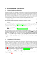
6 Measurements of other Sources
6.1 Galactic Synchrotron Radiation . . . . . . . . . . . . . . . . . . . . . . . . . . .
6.2 Astrophysical Radio Sources . . . . . . . . . . . . . . . . . . . . . . . . . . . . .
6.3 Non-Astrophysical Sources . . . . . . . . . . . . . . . . . . . . . . . . . . . . . .
44
44
44
45
3 Weather Conditions in Groningen
3.1 Data Aquisition . . . . . . . . .
3.2 Atmospheric Temperature . . .
3.3 Cloud Coverage . . . . . . . . .
3.4 Situation in Groningen . . . . .
.
.
.
.
.
.
.
.
.
.
.
.
.
.
.
.
.
.
.
.
4 Controlling the Telescope
4.1 Computer Control . . . . . . . . . . . . .
4.1.1 Arduino vs Raspberry Pi . . . . .
4.2 Controlling the Motor . . . . . . . . . . .
4.2.1 Stepper Motors . . . . . . . . . .
4.2.2 Communicating with the Motor .
4.3 Measurement Hardware and Control . .
4.3.1 Power Meter . . . . . . . . . . .
4.3.2 Temperature Monitor . . . . . . .
4.3.3 Communicating with the Devices
4.4 Operating the Telescope . . . . . . . . .
4.4.1 Connecting to the Telescope . . .
4.4.2 Observing with the Telescope . .
.
.
.
.
.
.
.
.
.
.
.
.
.
.
.
.
.
.
.
.
.
.
.
.
.
.
.
.
.
.
.
.
.
.
.
.
.
.
.
.
.
.
.
.
.
.
.
.
.
.
.
.
.
.
.
.
.
.
.
.
.
.
.
.
.
.
.
.
.
.
.
.
.
.
.
.
.
.
.
.
5 Measurements of the Sun
5.1 Solar Emission . . . . . . . . . . . . . . . . . . . .
5.2 Observing the Sun . . . . . . . . . . . . . . . . . .
5.3 Verifying the Beam Pattern . . . . . . . . . . . . .
5.4 Measuring the Brightness Temperature of the Sun
1
.
.
.
.
.
.
.
.
.
.
.
.
.
.
.
.
.
.
.
.
.
.
.
.
.
.
.
.
.
.
.
.
.
.
.
.
.
.
.
.
.
.
.
.
.
.
.
.
.
.
.
.
.
.
.
.
.
.
.
.
.
.
.
.
.
.
.
.
.
.
.
.
.
.
.
.
.
.
.
.
.
.
.
.
.
.
.
.
.
.
.
.
.
.
.
.
.
.
.
.
.
.
.
.
.
.
.
.
.
.
.
.
.
.
.
.
.
.
.
.
.
.
.
.
.
.
.
.
.
.
.
.
.
.
.
.
.
.
.
.
.
.
.
.
.
.
.
.
.
.
.
.
.
.
.
.
.
.
.
.
.
.
.
.
.
.
.
.
.
.
.
.
.
.
.
.
.
.
.
.
.
.
.
.
.
.
.
.
.
.
.
.
.
.
.
.
.
.
.
.
.
.
.
.
.
.
.
.
.
.
.
.
.
.
.
.
.
.
.
.
.
.
.
.
.
.
.
.
.
.
.
.
.
.
.
.
.
.
.
.
.
.
.
.
.
.
.
.
.
.
.
.
.
.
.
.
.
.
.
.
.
.
.
.
.
.
.
.
.
.
.
.
.
.
.
.
.
.
.
.
.
.
.
.
.
.
.
.
.
.
.
.
.
.
.
.
.
.
.
.
.
.
.
.
.
.
.
.
.
.
.
.
.
.
.
.
.
.
.
.
.
.
.
.
.
.
.
.
.
.
.
.
.
.
.
.
.
.
.
.
.
.
.
.
.
.
.
.
.
.
.
.
.
.
.
.
.
.
.
.
.
.
.
.
.
.
.
.
.
.
.
.
.
.
.
.
.
.
.
.
.
.
.
.
.
.
.
.
.
.
.
.
.
.
.
.
.
.
.
.
.
.
.
.
7 Future Improvements and Conclusion
7.1 Code Efficiency and Speed . . . . . . .
7.2 Reading Results from the Power Meter
7.3 Motor Power and Control . . . . . . . .
7.4 More Powerful Hardware . . . . . . . .
7.5 Conclusion . . . . . . . . . . . . . . . .
.
.
.
.
.
.
.
.
.
.
.
.
.
.
.
.
.
.
.
.
.
.
.
.
.
.
.
.
.
.
.
.
.
.
.
.
.
.
.
.
.
.
.
.
.
.
.
.
.
.
.
.
.
.
.
.
.
.
.
.
.
.
.
.
.
.
.
.
.
.
.
.
.
.
.
.
.
.
.
.
.
.
.
.
.
.
.
.
.
.
.
.
.
.
.
.
.
.
.
.
.
.
.
.
.
.
.
.
.
.
.
.
.
.
.
47
47
47
47
48
48
8 Acknowledgements
49
A Average Temperatures for June
52
B Average Cloud Coverage for June
57
C Telescope Server
62
D GPIB Communication
65
E Stepper Motor Control
68
F DNS Configuration
71
2
1
Introduction
A Short History of Radio Astronomy
Electromagnetic radiation can exist at any frequency. We are able to see signals coming from
high energy gamma or X-ray radiation all the way down to low energy radiation from radio
waves. Over time radio astronomy has come a long way and underwent a lot of changes.
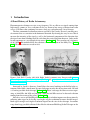
The first astronomical radio observation was made by Karl Jansky. He used a rotating array
of antennas that was sensitive in the horizontal direction. By rotating the array he was able to
measure the intensity of the signal as well as the horizontal component of the direction that
the signal came from. Nothing could be said about the vertical direction however. Janksy made
his measurements at a wavelength of 14.6 meters [Jansky, 1982]. This translates to a frequency
of 20.5 MHz1 . He concluded that the radiation came from a region of the Milky Way [Jansky,
1982]. His observation was made in 1933.
Figure 1: Left: Karl G. Jansky, 1905-1950. Right: Jansky’s antenna array. Images credit: https:
//en.wikipedia.org/wiki/Karl_Guthe_Jansky and http://www.nrao.edu/whatisra/
hist_jansky.shtml
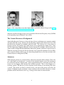
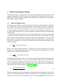
Interested by Jansky’s discovery, Grote Reber also started working in the field of radio astronomy. Reber built a much more advanced telescope to make his observations with. He built
a 9.5 meter parabolic dish telescope [Reber, 1944]. Reber’s telescope had three receivers operating at 3300 MHz, 900 MHz and 160 MHz. With the 160 MHz receiver he detected radiation
coming from the center of the galaxy [Reber, 1944].
Nowadays we are still building new radio telescopes to further improve our observations by
collecting more signal or by having even higher angular resolution for more detailed images.
Both signal strength and angular resolution depend on the size of the telescope. Inventions
range from large parabolic reflector dishes like the 100 meter Effelsberg Radio Telescope or the
1 Using
c = 299792458 m s−1
3
Figure 2: Left: Grote Reber, 1911-2002. Right: Reber’s parabolic reflector. Image credit: http:
//www.nrao.edu/whatisra/hist_reber.shtml
300 meter Arecibo telescope to large arrays of antennas like the Low Frequency Array (LOFAR)
or the upcoming Square Kilometer Array (SKA).
The Cosmic Microwave Background
After the Big Bang the Universe was hot and dense. Matter and photons were strongly coupled
and light could not escape. Minutes after the Big Bang atomic nuclei formed, but it was still
too hot for the electrons to recombine with the nuclei. The Universe was a hot plasma of
charged particles and photons and would remain so for approximately 380000 years. After
this the temperature dropped sufficiently for the electrons to recombine with the nuclei and
atoms to form: the Epoch of Recombination. Before this, photons could not escape because of
Thomson scattering, but now that the free electrons were captured the photons were less likely
to be scattered and they could escape. It is these first photons that we see when we look at the
Cosmic Microwave Background (CMB).
Antennas
When charged particles are accelerated they emit electro magnetic (EM) radiation. This is the
way radio signals are broadcasted. A current in the emitting antenna causes the electrons to
be accelerated and emit radiation with a power proportional to the acceleration squared. The
reverse can also happen. EM radiation can accelerate particles. This is what happens in a
receiving antenna. The EM wave causes electrons in the antenna to start moving and create
a current. This current can then be recorded and is a measure of the power received by the
antenna. With high angular resolution a source could be resolved and the radiation at various
positions could be measured to create e.g. an image of the source in radio emission.
4
The Project
The ultimate goal of this bachelor project is to measure the temperature of the CMB. To do this
we built a computer controlled horn antenna. Measurements will involve making sweeps of the
sky to measure the power as a function of elevation. The project was done by four students,
each of them focussing on some aspect of the telescope. The design of the horn was done by
Bram Lap [Lap, 2015]. Next Maik Zandvliet [Zandvliet, 2015] was in charge of constructing the
mount and mechanics of the telescope and for designing the back end where the electronics are.
I am responsible for the control of the telescope. I wrote the software necessary to both move
the telescope and provide a means to collect the data and I carried out observations of the Sun.
Finally Willeke Mulder [Mulder, 2015] focussed on calibration of the telescope to look into the
stability of the system and receiver temperature, which is crucial to know if we are going to
measure the CMB for which she also did the observations.
Summary
This thesis will present my contribution to the project. The first two chapters will cover material
that is not directly related to controlling the telescope, since during this time it was still under
construction. The material presented here is general information that is useful to know. In
Chapter 2, I will first look into some basic theory behind radio astronomy to see what kind
of signal we are actually receiving when doing observations and how the error in this signal
comes to be. Chapter 3 will next look into the weather conditions in Groningen and the effect
observing conditions have on the measurements. The fourth chapter will be a more practical
section about the electronics and the software for operating the telescope. Chapters 5 and
6 will present observations of the Sun and discuss the possibility of detecting other sources
respectively at 11 GHz. Lastly Chapter 7 will have a discussion about possible improvements
for the control of the telescope and about the results of the observations.
5
2
Radio Astronomy Theory
This chapter will give an explanation of what signal the telescope will receive and how it will
propagate through the system. The signal that comes in will be changed both due to atmospheric effects and noise effects within the receiver. For the best detection we want to minimize
these effects as much as possible.
2.1
Antenna Temperature
Measuring a received power is quickly done, however the data is unusable until it is calibrated
to a standard scale. In radio astronomy the signals are often calibrated against a temperature.
From a body with a known physical temperature we can measure the power it emits and use it to
set a scale for other measurements. The power received can now be related to a temperature, the
so-called antenna temperature. The antenna temperature is thus not the physical temperature
of the antenna.
The received power comes from all over the sky including other sources and even ground
emission. To get the total power we need to account for all of these contributions by taking
into account the power pattern of the antenna and the observed brightness of the sky. The
power pattern is a measure of how sensitive the antenna is to power from a certain direction.
To get the total power that is received we should thus convolve the observed brightness with
the power pattern:
Z
Ae
B (θ, φ)Pn (θ, φ) dΩ.
Pν =
2 4π ν
Here Pν is the received spectral power, Ae the effective area of the telescope, Bν the Planck
function, Pn the normalized power pattern and Ω the solid angle. The integration is over the
whole sky. As a temperature this becomes
Z
1
TA =
T (θ, φ)Pn (θ, φ) dΩ K,
ΩA 4π b
which follows from the fact that Pν = kT (see next section) and the Rayleigh-Jeans approximation of the Planck function Bν . Here TA is now the antenna temperature, ΩA the beam solid
angle, Tb the brightness temperature in some direction (θ, φ) and Pn the normalized power pattern in that direction. Finally, using the definition for the beam solid angle we get the following
expression for the antenna temperature [Wilson et al., 2013]:
R
Tb (θ, φ)Pn (θ, φ) dΩ
TA = 4π R
.
(1)
P
(θ,
φ)
dΩ
n
4π
The antenna temperature can be interpreted as the weighted average of the power received from
all over the sky. The sky brightness distribution is contained in Tb , the brightness temperature.
The power received from a certain position on the sky is now multiplied by the value of the
6
normalized power pattern Pn at that position. The normalized power pattern is 1 at its maximum
and decreases for the sidelobes. Sidelobes are positions outside of the main beam where the
response of the antenna is non-zero. The maximum is usually located in the center of the beam.
Therefore most of the power will come from the main beam. It is not possible to know from
what direction what power was received unless the observer knows there is a source at a certain
position. Therefore ideally we would want all of the power to come in through the main beam so
that we know exactly where the power is coming from. Hence reducing the sidelobes as much
as possible is a major part of designing a radio telescope to ensure the antenna temperature
incorporates only the signal of the source we want to measure and nothing else. For measuring
the CMB we will consider three components for the antenna temperature: the CMB itself, the
atmosphere and possible ground pickup. This results in a total antenna temperature of
TA = TCMB e−τ + Tatm (1 − e−τ ) + Tground [Mulder, 2015].
2.2
(2)
Noise and System Temperature
We consider all measured sources as noise sources. The telescope will thus measure a total
noise power Pν with associated noise temperature Tsys . Not all of the noise however comes
from external sources. Besides the power received by the antenna, there is also noise power
generated in the receiver itself with noise temperature TRx . The total noise temperature will
then be the receiver, TRx , temperature plus the antenna temperature,
(3)
Tsys = TA + TRx .
Here TA can include contributions from any noise source one can think of.
Tsys = TCMB + Tatm + Tsource + Tground + Tgalaxy + Tsun + · · · + TRx .
As we will see later on, for our observations we will only consider the CMB and the atmosphere
contribution of Eqn. 2. To eliminate the ground contribution the horn was designed with minimal sidelobes. Even if we were to pick up some ground, its contribution is negligibly small in
our case [Mulder, 2015]. In Chapter 6 we will see that the galaxy is also negligible. To relate this
system temperature to the measured power it is insightful to look at the origin of the receiver
noise, in particular that of the amplifiers.
2.2.1
Johnson-Nyquist Noise
The noise of the amplifiers in the back end comes from random thermal motions of electrons
inside the components. The random nature of this motion means that the average displacement
is zero, but the mean square displacement is not. Moving charges will
D Ecreate currents so the
motion of the electrons causes a small current I with hIi = 0, but I 2 , 0 to start flowing.
Higher temperatures will make the electrons move faster and thus the noise goes up. Cooling
the amplifiers properly can therefore reduce the produced noise. Because of its nature, this noise
is called thermal noise or Johnson-Nyquist noise after the two people that played an important
role in discovering and explaining this type of noise.
7
To find a relation between the measured power and the corresponding noise temperature
lets look at a resistor. Theoretically we can replace the noisy resistor with a noise source followed by a noiseless resistor. The noise power can be determined by loading a resistor R with
another resistor RL . The power that R puts into RL is then given by
D E
Pν = I 2 R = 4kT
RRL
[van Schooneveld, 1990].
(R + RL )2
This power is maximum when the loads are matched, i.e. R = RL . Now all factors except for
kT cancel out. We have now found a relation between power and temperature:
(4)
Pν = kTe .
Here Te is the effective temperature of the component. This can be equal to its physical temperature, but generally is not. It is important to note that this relation only holds for the spectral
power Pν . The power that the telescope will measure will be changed by both the bandwidth
and the gain. To convert this into a temperature we will need to correct for these before using
the above relation.
2.2.2
Propagation of Noise
Our telescope uses two amplifiers [Zandvliet, 2015]. Adding more amplifiers naturally adds
more noise which can get hard account for as the number of amplifiers increases. However, we
only have to consider the noise coming from the first amplifier. This has to do with where in the
chain the amplification happens. Consider a chain of n amplifiers with effective temperatures
Te,n and gains Gn . The output of an amplifier is Tout = G(Tin + Te ) [van Schooneveld, 1990].
The total noise temperature for n amplifiers is given by Friis formula[Wilson et al., 2013],
Te = Te,1 +
Te,3
Te,n
Te,2
+
+ ··· +
.
G1 G1 G2
G1 G2 · · · Gn−1
(5)
For a system consisting of two amplifiers this gives an effective temperature of
Te,sys = Te,1 +
Te,2
.
G1
Physically this means the following. The noise added by later amplifiers is with respect to an
already amplified signal. This implies that the true noise added by this amplifier is its noise
temperature divided by the gain of the previous amplifiers. From Eqn. 5 it becomes clear that
this rapidly makes the noise added by later amplifiers negligible. If amplification in the first
stage is high enough we can even consider the noise of the second amplifier to be negligibly
small, because of this only the noise of the first amplifier is important.
8
2.3
Sensitivity and Integration Time
In the previous section we saw that a radio telescope measures a total temperature Tsys at its
output given by Eqn. 3. This temperature has a RMS uncertainty, σT , associated with it given
by
Tsys
.
σT = √
∆ν t
(6)
The quantity σT is called the sensitivity of the telescope, ∆ν is the receiver bandwidth and t the
integration time, i.e. how long signals are collected for a measurement. The smallest signal that
can be detected is a signal that is σT higher than these RMS fluctuations. Sources of interest
are often weaker than the noise sources, so good sensitivity is a major plus for an observation.
Looking at Eqn. 6 we see that we can increase the sensitivity in three ways.
• Decrease System Temperature: Creating a system that has a low noise level will lower
Tsys and make the system more precise.
• Increased Bandwidth: With a large bandwidth the telescope will receive power from
a wider spectrum and therefore sensitivity is increased.
• Longer Integration Time: By observing the source for a longer time more signal is
collected, increasing precision.
To get an understanding of how Eqn. 6 comes to be we look at what σT actually is. The
system temperature Tsys can be seen as a noise temperature with all signals to be coming from
noise sources. The random nature of this signal results that we are in fact measuring the vari2
ance of a random
√ signal with noise. Measuring the variance σ of random samples has an
uncertainty of 2σ . This gives the first part of the equation,
√
σT = 2Tsys .
For the denominator we need the Shannon sampling theorem and the Central Limit Theorem. The sampling theorem provides the minimum frequency one needs to sample a signal at
in order to completely reconstruct it. It states that if a signal has a frequency f then one can
reconstruct this signal completely by sampling it at a rate 2f [Jerri, 1977]. Suppose an incoming signal with a bandwidth ∆ν. The theorem then implies this signal needs to be sampled at
2∆ν. After a time t we will have collected a number of samples
√ N = 2∆νt. Finally the Central
Limit Theorem tells us that the uncertainty in Tsys drops as N , with N being the number of
measurements. This will give
√
2Tsys
σT = √
,
2∆νt
thus yielding Eqn. 6.
9
2.4
Applying the Theory to the Kapteyn Radio Telescope
The horn is a Pickett-Potter horn design about 30 cm in length. The receiver is built to receive
signals at 11 GHz with a bandwidth of 1.05 GHz, going from 10.45 to 11.5 GHz. This means we
are looking at signals with a wavelength of 2.7 cm [Lap, 2015; Zandvliet, 2015]. This section
will apply the theory discussed above to the telescope to get a feeling for the quantities we will
be dealing with.
Antenna Temperature and CMB Brightness
The main purpose of this telescope was to be able to measure the temperature of the CMB. The
CMB is a near perfect black body radiating at a temperature of TCMB = 2.72548 ± 0.00057 K
[Fixsen, 2009]. For designing the back end it is important to know what order of power we are
receiving. Black body radiation is characterized by the Planck spectrum,
1
2hν 3
,
Bν (T ) = 2
c exp(hν/kT ) − 1
(7)
where h is Planck’s constant; ν is the observing frequency; c is the speed of light; k is the
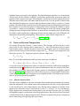
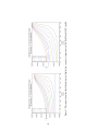
Boltzmann constant and T is the temperature of the black body. Figure 3 shows the spectrum
of the CMB. The peak of the signal lies at a frequency of ν = 160 GHz. At this frequency the
CMB has a brightness of Bν = 3.88 · 10−16 W Hz−1 m−2 sr−1 . The available hardware however
will limit us to a range of frequencies between 4 and 11 GHz. In Fig. 3 we see that this range is
at the faint end of the CMB spectrum. Therefore, we chose the highest possible frequency of 11
GHz. This gives a brightness of Bν = 9.29 · 10−18 W Hz−1 m−2 sr−1 . The atmosphere will both
attenuate the CMB signal and add to the signal [Mulder, 2015]. This will result in an antenna
temperature of
(8)
TA = TCMB e−τ + Tatm (1 − e−τ )
Assuming TCMB = 2.72584 K, Tatm = 283 K and τ = 0.05 (see Mulder [2015]) when looking
at zenith we can make an estimate of the antenna temperature and the received power. Using
Eqn. 8 the antenna temperature is TA ≈ 16.4 K. The incoming power follows from multiplying
Eqn. 4 with the bandwidth. The effective temperature now is a combination of the antenna
temperature and the receiver temperature.
P = k(TA + TRx )∆ν
If we assume a receiver temperature fo TRx = 200 K this gives an incoming power of P =
3.13 · 10−12 W or P = −85.03 dBm using k = 1.3807 · 10−23 J K−1 and ∆ν = 1.05 GHz. The
measuring range of the power meter extends from −70 dBm to +20 dBm [Agilent Technologies,
2013a]. Our system uses two amplifiers of around 30 dB each [Zandvliet, 2015]. If we assume the
system gain comes only from the amplifiers and is 60 dB this results in a signal of approximately
−25.03 dBm.
If the optical depth decreases to τ = 0.01 the antenna temperature drops to 5.5 K. Using the
same value for the receiver temperature and gain the power becomes P = −25.26 dBm. The
10
Figure 3: Top: the brightness Bν of the CMB as given by the Planck function for TCMB =
2.72584 K. Bottom: a zoom of the available frequency range, showing the expected Bν ∝ ν 2
property of the Rayleigh-Jeans law.
final signal will be somewhat different because of effects of the other components, cables, the
horn and changes in both atmospheric and receiver temperature, but it will be around these
values.
Noise and System Temperature
We assumed before that the noise produced by the second amplifier is negligible. Here we show
this is not the case. The noise temperature of the second amplifier, ALMA2, has an average value
of 127.35 K [Zandvliet, 2015]. Using Eqn. 5 its final contribution would then be 4.25 K. The
noise temperature of the first amplifier, MITEQ, is 110.90 K. Since the CMB has a temperature
of 2.7 K, a noise of 4 K on 110 K is in this case not negligible. This is all taken in however in
the measurement of the receiver temperature. The noise temperature of the back end will thus
lie close to the noise of the two amplifiers combined. The noise temperature of the back end is
measured by Zandvliet [2015].
11
Sensitivity and Integration Time
The noise temperature of the system allows us to make a prediction of our sensitivity. If we
want to be able to measure the temperature of the CMB to 10% accuracy, the upper limit on
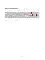
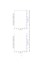
the sensitivity will be as follows. Thus, the limit is set on 0.2 K. Eqn 6 depends linearly on
Tsys . As the receiver temperature fluctuates, so will the sensitivity. We measured the receiver
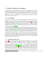
temperatures ranging from around 180 K to around 200 K. Looking at Fig. 4 and Fig. 5 we see
that for a sensitivity of 0.2 K the integration time will be of the order of milliseconds. Even in
bad conditions with high optical depths this is still the case. The low integration times tell
us that our measurements will not be limited by the system noise. Instead the limiting factors
will be how well we can determine the other quantities like the atmospheric temperature, the
opacity and the receiver temperature.
12
13
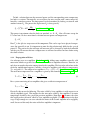
Figure 4: The sensitivity as function of integration time for a receiver temperature of 180 K (left) and 200 K (right).
14
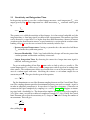
Figure 5: The integration time for different optical depths for a receiver temperature of 180 K (left) and 200 K (right).
3
Weather Conditions in Groningen
Despite being able to reach our requirements even in relatively bad circumstances, we still
want the observing conditions to be as good as possible. In Groningen we have two main
concerns: the atmospheric temperature and the cloudiness. In this chapter an estimate of what
is approximately the best observing moment in Groningen will be made. It is not insightful to
pinpoint an exact date, so we will limit the investigation to find an approximate best time of
the year and time of day to observe.
3.1
Data Aquisition
To be able to get a good overview of the weather in Groningen we need data that spans over
multiple years. To do this we use data from the KNMI, the institute that monitors the weather
throughout the Netherlands. These data are publicly available on the website2 . It is also possible
to request the data through a script, which is the way it was done here. With the available data
it is possible to go all the way back to the previous century. In this case we will use the data
from 2007 till 2015. Since there is no weather station in Groningen we will use the data from
the nearby station in Eelde [KNMI].
The data from the KNMI is available in either daily measurements or hourly measurements.
We used the hourly measurements to have the greatest flexibility. The KNMI tracks all sorts of
data such as windspeed, sunshine, precipitation, cloud coverage and temperatures. For us only
the cloud coverage and temperature data are important. When reading data from their database
it should be taken into account that all the temperatures are presented in units of 0.1 °C and
hence needs to be converted to units of 1 °C first. Cloud coverage is expressed in special units
of oktas or octants. This unit indicates how many eights of the sky are covered in clouds. It
ranges from 0 to 8, with 0 octants meaning clear skies and 8 octants meaning a sky completely
covered in clouds. In some situations the sky may not be visible at all, such as with dense fog.
In this case the cloud coverage gets a 9.
3.2
Atmospheric Temperature
Equation 8 for the antenna temperature shows that the atmosphere increases the signal with
unwanted noise and does so inverse exponentially. With e−τ = 0.95 for τ = 0.05 the contribution from the atmosphere may seem small, but because the atmospheric temperature is high
relative to the CMB and other sources, the Tatm (1 − e−τ ) term still contributes significantly,
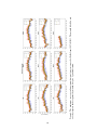
typically ranging from 3-10 K [Mulder, 2015]. We therefore aim for an atmospheric temperature that is as low as possible. In Fig. 6 we have plotted the minimum, average and maximum
temperature for every day of the year. The distribution looks roughly the same every year. We
can see that the highest and lowest temperatures are during the summer and winter months
respectively. For a more clear view we calculated the minimum, average and maximum temper-
2 http://www.knmi.nl/klimatologie/uurgegevens/selectie.cgi (hourly) or http://www.knmi.nl/klimatologie/daggegevens/download.h
(daily).
15
16
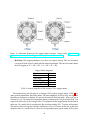
Figure 6: The minimum, average and maximum temperature as measured at Eelde from 2007 till 2015. The month labels do not
exactly separate the data points by month, but give a good indication.
17
Figure 7: Minimum (blue crosses), average (yellow dots) and maximum (red crosses) temperatures for each month separated by
year. The errorbars give the standard deviation of the average.
Minimum
Average
Maximum
2007
9
16.98
30.1
2008
4.3
16.25
29.4
2009
2.7
14.73
25.9
2010
2.7
15.15
28.3
2011
4.0
15.57
31.3
2012
4.8
14.18
25.6
2013
6.8
14.48
28.4
2014
4.2
15.59
26.6
Table 1: Minimum, average and maximum temperatures in June per year in °C.
ature per month. This is shown in Fig. 7. From these plots we can see that the coldest months
are January, February and March.
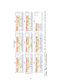
We will be doing our observations in June however. Table 1 shows the minimum, average
and maximum temperatures of June for the past years. The average temperature is around 1516 °C, but the minimum and maximum are far apart. For a better view of how the temperature
is spread across the day we will look at different parts of the day separately. We define night
(00:00-06:00), morning (06:00-12:00), afternoon (12:00-18:00) and evening (18:00-00:00). Figure 8
shows this for June 2014. For the other years see App. A.
Hourly the temperatures can fluctuate strongly and this varies on a daily basis, however
from these figures we do see that in general the night time is the coolest part of the day. Temperature wise observing conditions are best during the night.
3.3
Cloud Coverage
Even more important than the atmospheric temperature is the cloud coverage. When there is
a cloud in the field of view of the telescope the opacity of that area can increase dramatically.
For larger optical depth the factor e−τ becomes increasingly smaller. This reduces the signal
from the CMB and increases that of the atmosphere. For comparison, the contribution of the
atmosphere is 2.97 K for τ = 0.01 while it is 14.53 K for τ = 0.05, assuming Tatm = 298 K.
Besides increasing the opacity, clouds will also make it non-uniform over the area of the beam.
This adds another complication in accounting for the contribution from the atmosphere.
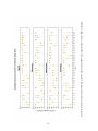
In Fig. 9 we see the cloud coverage as measured by the station in Eelde. We see that the data
is spread out through the plot filling the entire 0 to 9 scale. It does however seem to tend to the
higher cloud coverage values on average.
To get a better view of the data we took the average per month. The results of this are
shown in Fig. 10. This confirms the earlier statement of higher overall cloud coverage. Even
in the months that were good in terms of atmospheric temperature, the sky is still covered in
clouds for the most part. This is not completely unexpected. Even if there would be days of
little to no cloud coverage these are averaged out by days of high cloud coverage. It would be
quite rare for an entire month to have a low cloud coverage.
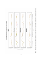
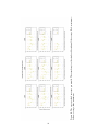
Finally we split the data by part of the day like for the temperature to see if it changes
significantly. Figure 11 demonstrates this, but the results are inconclusive. Appendix B has the
plots for the other years but they do not give usable information either.
18
19
Figure 8: Temperatures of June 2014 separated by part of the day. From top to bottom: night, morning, afternoon and evening.
20
Figure 9: Cloud coverage in octants for all days of the year. The month labels are not exact but give a good indication. Red:
maximum; Yellow: average; Blue: minimum.
21
Figure 10: The average cloud coverage per month. The errorbars give the standard deviation of the average. Red: maximum;
Yellow: average; Blue: minimum.
22
Figure 11: Cloud coverage of June 2014 separated by part of the day. Red: maximum; Yellow: average; Blue: minimum.
3.4
Situation in Groningen
The two most important factors of the weather are atmospheric temperature and cloud coverage. It turns out we have limited control over the first one. We can make a rough estimate
of when the temperatures will be lowest and hence best for observing. This is in the winter
months January, February and March. Further, breaking it down and looking at the time of
day, we also saw that night time has the lowest temperatures. The best observing date and
time would therefore be sometime in the winter during the night (i.e. 00:00 - 06:00). We will be
observing in June, but the night time will still have the lowest temperatures. Cloud coverage on
the other hand is beyond our control. Due to its changing nature we cannot make an estimate of
a best observing moment. The best moment for this would need to be decided by the observer
by checking the weather conditions.
Although this analysis has given some insight in the weather conditions, it still remains
difficult to find reliable correlations between observing time and cloud coverage. For the best
observing time it comes down to checking the weather forecast or the weather outside directly
to see if conditions are and will stay suitable.
23
Arduino Uno
Processor
ATMega328
Voltage
5V/7-12V
CPU Speed 16 MHz
SRAM
2 kB
Raspberry Pi B+
Processor
Broadcom BCM2835 SoC
Voltage
5V
CPU Speed 700 MHz
SDRAM
512 MB
Table 2: Arduino Uno and Raspberry Pi B+ specifications.
4
Controlling the Telescope
4.1
Computer Control
Our measurements will involve moving the telescope over a strip in the sky in elevation. To
make a reliable measurement we decided to mount the horn on a frame and control the telescope with a computer. The telescope moves with a motor and power is read digitally from a
powermeter. This gives us a couple of advantages. First of all the mount will ensure that we
start and end in the same strip of the sky. This way we only have to worry about the received
power as function of elevation, easing the data reduction later on. Secondly we will control
the speed factor. Using a motor controlled by a computer ensures that each measurement will
be taken in the same amount of time. This way data collection is consistent for every measurement. Lastly it makes determining the received power at a certain angle easier and more
reliable. A full computer would be too large to fit into our build so we opted to go for something
smaller. This gives us the choice between an Arduino and a Raspberry Pi.
4.1.1
Arduino vs Raspberry Pi
The telescope will be rotated by a stepper motor. Controlling the motor is a simple task and
can be done by a simple system, but maybe expansions are desired in the future needing a more
advanced system. To make a decision we compared the two devices with each other. Table 2
lists the specifications of the Arduino Uno and Raspberry Pi B+ respectively.3 It immediately
shows that a Raspberry Pi (from here on "Pi") is much more powerful than an Arduino. This
is because there is a key difference in how they operate. The Arduino has a microcontroller. It
has no OS, it just runs its code when told to do so. The Pi however is a full computer complete
with OS.
Programming the Arduino would (in principle) require programs in C and the programming
would be indirect. One would write the code and upload it to the microcontroller. It would then
be able to do the one thing the program was written for. Programming the Pi can be done in
Python on the machine itself. This has multiple advantages. For one, Python is a flexible and
easy to use programming language, making developing with it much more convenient. Being
able to program on the device itself is also a plus for quickly making small changes later on.
3 Arduino specifications are taken from http://www.arduino.cc/en/Products.Compare.
ifications are taken from https://www.adafruit.com/datasheets/pi-specs.pdf
24
Raspberry Pi spec-
Finally the Pi is the most future proof should upgrades, e.g. more sensors, be desired in the
future. It is for these reasons that the telescope will be controlled by a Raspberry Pi B+.
4.2
Controlling the Motor
4.2.1
Stepper Motors
To control the elevation of the horn we used a stepper motor. A stepper motor divides a full
rotation into a number of steps of equal size. Applying an electrical pulse moves the motor
one step. This allows for the precise control of the position of the motor. Since it moves in
discrete steps we can determine its position simply by counting the number of pulses we sent
to it. This eliminates the need of external tools for measuring the position. There will be an
error associated with the angle moved due to the possibility of missed steps. A great property
of stepper motors is that this error is non-cumulative. One step will therefore have the same
error as a million steps [Ericsson]. We will not account for this error in the position. The reason
for this is that we tested the motor multiple times by letting it move to various angles and then
return to the park position many times. It had not missed any steps during the tests, so the
error is negligible.
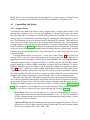
A stepper motor consists of two parts: a stator and a rotor. Figure 12 shows this basic
structure. The stator is the outer ring consisting of electromagnets with teeth. Each pair of
opposing poles of electromagnets is called a phase. Most common is the 2-phase stepper motor.
Adding more phases will give a higher resolution, i.e. a smaller angle per step. Recently, 5-phase
stepper motors have achieved higher resolutions and more steps per revolution. A 2-phase
motor has four poles per phase, while a 5-phase motor, for example, has two poles per phase.
In Fig. 12 we see a 2-phase and a 5-phase motor with the phases labeled. It might seem that the
2-phase motor actually has four phases, but this is because it are actually two motors together.
For 2-phase motors the coils usually have a center tap, which allows for easy reversing of the
magnetic poles without switching the current direction. This is called a unipolar motor.
The rotor is the inner disk. This disk has magnetized teeth, all coming in north-south pairs.
Once a phase is turned on some of these teeth on the rotor will be out of alignment with those
on the stator. Magnetic forces will now pull the rotor in alignment with the stator: the step.
To move the motor the phases are turned on and off in a certain sequence [Orientalmotor,
2015]. These sequences are determined by so-called drive methods. There are three main drive
methods: wave drive or 1-phase full step, 2-phase full step and half step [Ericsson].
• Wave Drive: Wave drive has one phase on at a time. It is the simplest way to drive a
stepper motor and the coil activation scheme would be A → B → Ā → B̄. The downside is
that for a unipolar motor this way does not give maximum torque because only a quarter
of the coils is used at any time.
• 2-phase Full Step: For maximum torque the 2-phase full step scheme is better. This way
two phases are on at all times, using half of the available coils. The coil activation scheme
for this drive method is AB → BĀ → ĀB̄ → B̄A.
25
Figure 12: Schematic drawing of the stepper motor structure. Image credit: http://www.
orientalmotor.com/technology/articles/2phase-v-5phase.html
• Half Step: Half stepping combines wave drive and 2-phase driving. This way the motor
can rotate half the angle it would with the other two methods. The coil activation scheme
for half stepping is A → AB → BĀ → Ā → ĀB̄ → B̄ → B̄A
Stepper Motor Properties
Type
Unipolar
Phases
2
Step Angle
1.8°
Holding Torque
9 N cm
Operating Voltage 12 V
Steps per Rev.
200
Table 3: General properties of the Astrosyn Y129 stepper motor.
The motor driving the telescope is an Astrosyn Y129 2-phase stepper motor. Table 3 lists
some general information about this motor. The most important is that it takes 200 steps for
the motor to make one revolution. We operate the motor in half step mode. With each step it
will move by 1.8°. To mount the telescope the motor is connected to a larger rotatable disk. Our
supervisor told us that in this setup it takes 72 revolutions of the stepper motor for the disk to
make one. We verified this by marking the disk and then sending 200 · 72 pulses to the motor.
This means with each step our telescope will move 0.025° or 90 arcsec on the sky. In between
the pulses there is a small delay of 2 ms or 1.3 ms depending on the speed setting. If the pulses
26
arrive too fast the motor will not have time to respond and it will hang. It takes the horn 80
seconds to do a measurement with a 1 degree step and 32 seconds with a 13 degree step both
at the fastest mode.
4.2.2
Communicating with the Motor
To control the motor we use the General-Purpose Input/Output (GPIO) pins on the Raspberry
Pi. The stepper motor controller we use has a 15-pin connector, but we only need three pins:
ground, step and direction. These pins are connected to a ground pin and two GPIO pins on
the Pi respectively. We cannot however directly connect the motor controller to the Pi, as the
GPIO pins run at 3.3 V while the controller needs 5 V. If the 5 V would flow into these pins the
Pi could possibly get damaged. To prevent this from happening we made a special connector
with Zener diodes connecting the step and direction pins to ground. A Zener diode allows
current to flow backwards once a certain breakdown voltage is exceeded. The connector has
two 3.3 V Zener diodes. If the voltage over the Zener diode now exceeds 3.3 V the current will
flow towards ground. The schematic for the socket is shown in Fig. 13. These three wires are
then connected to the following pins on the Pi: 29, 31 and 30 for direction, step and ground
respectively. The pins on the Pi can be set either high (3.3 V) or low (0 V). For movement, we
set the direction pin either high or low to move forwards or backwards. Next the step pin is
continuously switched between high and low. Every time the step pin is powered the motor
will move one step. After testing with a prototype of loose wires, a custom cable was made
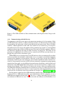
which can be seen in Fig. 14.
Figure 13: Schematic for the connector connecting the motor controller to the Pi. The connector
is a 15 pin female D-Sub connector.
27
28
Figure 14: The cable connecting the motor controller box to the Raspberry Pi. Left: the inside of the connector showing the
wires and the Zener diodes. Right: the complete cable with aluminium case and connector for the GPIO pins.
4.3
Measurement Hardware and Control
To measure the power received by our telescope we use an Agilent E4412A power sensor connected to a Agilent E4418B power meter. These devices are shown in Fig. 15. To measure
temperatures we use a Lakeshore 218S Temperature Monitor for reading out the sensor, see
Fig. 16. To save the measurements we have to set up a connection between the Pi and the
devices so we can read out values and store them.
Figure 15: The equipment used for measuring the power. Left: power meter. Right: power
sensor. Image credit: http://www.sglabs.it/ and http://www.us-instrument.com/
Figure 16: The Lakeshore 218S Temperature Monitor used for reading out the sensor. Image credit: http://www.lakeshore.com/products/cryogenic-temperature-monitors/
model-218/pages/Overview.aspx
29
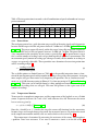
Table 4: The integration time in seconds as for all combinations of speed and number of averages
per measurement.
Speed
1
0.05
0.025
0.005
20
40
200
4.3.1
2
0.1
0.05
0.01
4
0.2
0.1
0.02
Readings Averaged
8
16
32
64
0.4 0.8 1.6 3.2
0.2 0.4 0.8 1.6
0.04 0.08 0.16 0.32
128
6.4
3.2
0.64
256
12.8
6.4
1.28
512
25.6
12.8
2.56
1024
51.2
25.6
5.12
Power Meter
The used power meter has a wide detection range capable of detecting signals with frequencies
between 100 kHz up to 110 GHz and powers between -70 dBm and +44 dBm [Agilent Technologies, 2013a]. The power sensor falls nicely within this range, being able to measure frequencies
between 10 MHz and 18 GHz and powers between -70 dBm and +20 dBm. The power meter is
a key component in the sensitivity of our system as given by Eqn. 6. The power meter is set to
take a certain number of readings and average them together to produce a measurement. The
measurement speed (amount of readings per taken per second) and the number or readings to
average are separately adjustable. These quantities now determine what our integration time
will be according to Eqn. 9.
τ=
readings averaged
measurement speed
(9)
The available options are limited however. Table 4 lists the possible integration times as function of the measurement speed and the number of readings averaged for a measurement. Averaging
more samples will give lower noise levels improving the precision. For an absolute measurement it is ±0.02 dB when measuring in dBm or 0.5% when measuring in W [Agilent Technologies, 2013a]. This error can be brought down by taking multiple measurements, i.e. changing
the number of readings that are averaged. The error will go down as the square root of the
number of readings.
4.3.2
Temperature Monitor
To measure the atmospheric temperature and the temperature of the hotload we use a Pt1000
sensor. It operates between -50°C and +150°C with tolerance class 2B. This means the sensor
has an accuracy given by
σ = ±(0.6 + 0.005|t|) [Heraeus, 2013].
(10)
Note that t should be in °C. Outside this range the sensor still functions but the uncertainty
becomes larger and it might damage the sensor due to material stresses. To connect the sensor
to the temperature monitor another cable was made which can be seen in Fig. 17.
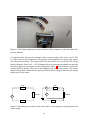
The temperature is determined by measuring the resistance of the sensor. This introduces
a problem: wires have resistance. If we were to construct a circuit as in the left of Fig. 18
30
Figure 17: The Pt1000 temperature sensors with the cable to connect it to the Lakeshore temperature monitor.
we would not only measure the resistance of the sensor, but that of the wires as well. This
is a direct error in the measurement. The solution to this problem is to separate the current
and voltage measurements. The current will be the same since it is a series circuit. The voltage
however drops by Ohm’s law V = IR. To eliminate the wire resistance one should only measure
the voltage drop over the sensor as in the right picture of Fig. 18. This is known as four-wire
sensing or Kelvin sensing. The wires to the voltmeter only carry a tiny current. The voltage
drop caused by them can therefore be neglected. The measured voltage is now only the voltage
drop caused by the sensor.
wire
A
Pt1000
wire
V
Pt1000
Ω
wire
wire
Figure 18: Measuring the resistance of the sensor (left) vs. measuring the voltage drop over the
sensor (right).
31
Figure 19: The GPIB controller to allow communication with the power meter. Image credit:
Prologix
4.3.3
Communicating with the Devices
To communicate with the power meter and temperature monitor we had two options: RS232
or GPIB. The Pi does not have an RS232 interface, but there are USB converters so that would
be no problem. Our supervisors advised against RS232 for two main reasons. First of all RS232
would be a difficult protocol to work with. One would have to account for e.g start/stop bits,
the number of data bits sent or the number of bits transmitted per second. A second problem
would arise when using an RS232 to USB converter. The name by which the computer addresses
the USB device depends on the order in which all devices are plugged in. The names are not
persistent, so if multiple devices will be used we cannot be sure that the next time devices are
plugged they will have the same names again.
GPIB or IEEE-488 was developed in 1974 by HP for devices that can automatically test other
devices or perform measurements automatically. It was an attempt to standardize communication between computers and instruments. With the General Purpose Interface Bus (GPIB) all
instruments would have the same connector. Later with the introduction of the Standard Commands for Programmable Instruments (SCPI) all devices obtained a common basic programming
command set along with a set of guidelines for manufacturers should they wish to include new
commands. Using GPIB multiple measuring devices can easily be used and is as simple as daisy
chaining them together. This is because each device has its own address for communication.
Two limitations should be considered however. Each device can have an address between 0 and
30, but a driver can only drive 14 devices at a time. Second, the cable length should not exceed
20 m in total or 2 m between devices for maximum data transfer rates. ICS Electronics [2009]
For this project it turned out that GPIB connection would be the easiest to work with. The
Pi does not have a GPIB connector either, so to communicate with the equipment we use a
GPIB-Ethernet controller shown in Fig. 19. This acts as a bridge converting signals received
over ethernet to GPIB and vice versa. To read out results one connects to the controller via an
32
ethernet cable. Before commands can be sent we need to set up a connection with the controller.
This is done by setting up a TCP connection at port 1234 at the controllers IP address [Prologix,
2013]. In Python this is easily done using sockets in the socket module. The details can be seen
in Appendix C. The equipment can now be read out by sending the appropriate commands
over the socket. When talking to a device two things should be accounted for. Commands
should always be terminated by the newline character \n. This indicates you are done sending
the command and that it can start processing it. The second is the way sockets work. In the
Python documentation they warn the user that when sending or receiving a message, you may
not send or receive the entire message in one call. It is the users responsibility to make sure
everything is sent or received. Sending the entire message can be done with the socket module
itself by using the socket.sendall method. Commands are then sent to the controller which
processes them and queries the power meter for a response. However there is no such method
for receiving. To make sure we receive everything the power meter sends us we keep querying it
for more data until it returns None indicating there is nothing more to send. The code governing
communications with the GPIB controller and the powermeter can be found in GPIBComm.py
in Appendix D. The fact that we can use ethernet influenced the decision on how to operate
the telescope. This is discussed in the next section.
4.4
Operating the Telescope
There are many question as to how the telescope can be operated. Should the measurements be
automatic to eliminate user error? Should the operator have input? If so, to what extent? How
will the user interface look like? What preliminary knowledge does the user need to have?
These are all questions to consider when thinking about the interface to the telescope. The
telescope will possibly be used for the astronomy bachelor course Radio Astronomy in the third
year. Thus it will mainly be students operating the telescope.
The Pi has four USB ports and an HDMI port so the first idea was to simply have a monitor,
keyboard and mouse. During the frame design however (see [Zandvliet, 2015]) it became clear
this would not be ideal. It has too many downsides. Having many peripherals would mean one
would need to access the Pi frequently for connecting and disconnecting and we would need a
way to handle all the cable work. It also meant carrying many things alongside the telescope.
This would compromise portability a lot. Furthermore the whole setup would become just too
bulky. All these situations make the setup less user friendly, so we discarded this idea.
Thinking about the portability led us to consider the operator controlling the telescope
from his or her own laptop. The only problem was then how the communication between the
Pi and the laptop would work. The only ethernet port was taken by the GPIB controller and
there are no other connections. Connecting everything by ethernet does solve the problem of
not knowing what device has what name, since everything gets an IP address. We thought of
setting up a small LAN network depicted in Fig. 20. The network would consist of the following
components:
• Raspberry Pi
• GPIB-Ethernet controller
33
Figure 20: The LAN network connecting all devices in the telescope with each other.
34
• User laptop
• Network switch or router
The switch or router will provide the ethernet ports to connect everything together. The Pi will
take care of communication between the user’s laptop and the system.
4.4.1
Connecting to the Telescope
To operate the telescope the user will connect a laptop to the router or switch. To deal with the
IP addresses we have two choices: configure the Pi to handle them or use a router. While the
router might save us some work, we chose to configure the Pi to act as a DHCP server and hand
out the IP addresses. To do this we used the dnsmasq tool, a free DNS forwarder and DHCP
server. The configuration file is in Appendix F. The network was set up in such a way that the
Pi and the GPIB controller have a static IP so that we know for sure they are at those addresses.
The address of the laptop is not important as we do not need to address it. The user should
now establish an SSH connection to the Pi. The IP addresses are set as 192.168.0.15 for the Pi
and 192.168.0.142 for the GPIB controller. The Pi now automatically assigns addresses between
192.168.0.20 and 192.168.0.100 to other connecting devices. All scripts are executed on the Pi.
They should therefore either be written on the Pi or be transferred to it beforehand. Normal
observers should connect to the Pi with the observer account with password observer.
4.4.2
Observing with the Telescope
Once logged in the user should change directories to the Desktop folder where the main script
for controlling the telescope is located: ScopeServer. This script should be run with the sudo
command otherwise control through the GPIO pins is not possible. When run, the script will
try to have all GPIB connected devices identify themselves to make sure all the required devices
are there. If you see a None response it means a command did not receive a response and the
connection should be checked. Once the identifiation finishes you will see a prompt starting
with >>> . From here the user can either control the telescope directly or run a script. The
commands for direct control are listed in Table 5.
When making a sweep of the sky it is not ideal to simultaneously measure the power and
the atmospheric temperature. Measuring simultaneously will interrupt often the sweep and
therefore cause the motor to stop or even miss a step. When the motor misses a step the angle
of the horn will be off and the data becomes unusable. Instead it should be measured at one of
the loads or set the temperature monitor to log the data and retrieve it later on.
35
Table 5: A list of commands available to the observer for manual control.
Command
!calib
park
prep
rot h±angi
!rot h±angi
run hscripti
speed hrpsi havgsi
speed?
turbo h0|1i
Description
Forces recalibration of the zero position.
Returns the telescope to its zero position.
Points the telescope to the cold load.
Rotates the telescope by the given amount of degrees. Will give an error
when attempting to move out of bounds (i.e. below 0 or above 180 degrees).
The same as rot but it ignores the limits. Use this with caution.
Executes the script. Name should be given without the .py extension.
Changes the setting of the power meter. rps sets the readings per second.
avgs sets the number of readings averaged for a measurement.
Queries the current speed setting.
Switches speed settings for rotation.
36
5
Measurements of the Sun
The ultimate goal of this telescope is to measure the temperature of the CMB. It is nice to check
though if we could observe more sources with it. The Sun for example is a near, bright source
so it would be nice to see if we are able to measure it with our telescope. We also look into the
possibility of detecting some of the brightest radio sources in the sky besides the Sun.
5.1
Solar Emission
Emission from the Sun has multiple origins. Charged particles accelerated in the Sun’s magnetic
field will emit radiation via mechanisms such as synchrotron radiation, free free emission or a
form of gyro radiation. This is mainly important for sunspots however. The conditions in these
areas allow for gyro-resonant emission which is an efficient emission mechanism coming from
electrons rotating around the magnetic field lines [Lee, 2007]. Another part of the emission
comes from thermal radiation. If we consider the Sun to be a black body with a temperature
equal to its surface temperature, it will radiate according to Planck’s law (Eqn. 7) with T =
5778 K.4
Sunspots are part of the active Sun, while the thermal emission comes from the quiet Sun.
Fig. 21 shows spectra of different sources. We see that at 11 GHz the contribution of the active
Sun and quiet Sun are nearly equal and becomes a straight line. The plot is in log scale so a
straight line means a power law relation. In the Rayleigh-Jeans limit (hν kT ) the Planck
function reduces to a power law resulting in a line with slope 2,
Bν (T ) =
2kT ν 2
c2
(11)
The radiation we measure with our telescope is thus mostly that of the quiet Sun. Based on its
temperature we can estimate the brightness of the Sun and the power that we will receive. To
find the power we receive from an object, we multiply the brightness (Bν ) with the solid angle
of the object (∆Ω), the effective area of the telescope (Ae ) and the bandwidth (∆ν) giving
(12)
P = Bν ∆ΩAe ∆ν.
The estimated brightness is Bν = 2.15 · 10−16 W Hz−1 m−2 sr−1 . The solid angle of the sun
can vary slightly, so we use its size at a distance of 1 AU: 1919 arcsec.4 This gives a solid
angle of ∆Ω = 6.8 · 10−5 sr. The effective area of our telescope is 0.023516 m2 [Lap, 2015]
and our bandwidth is 1.05 GHz. This gives an expected power of P = 3.61 · 10−13 W or
P = −94.42 dBm. Combined with the CMB and the atmosphere mentioned earlier in Chapter
2, we expect a total power of P = −84.55 dBm arriving at the antenna when pointing at the
Sun with an optical depht of τ = 0.05. The gain of the telescope is around 60 dBm so this will
be well within the observable range and we are able to measure the Sun. By measuring the Sun
we can do two interesting experiments. We can try to measure properties ofthe main beam and
we can try to determine the brightness temperature of the Sun.
4 NASA
Sun Fact Sheet: http://nssdc.gsfc.nasa.gov/planetary/factsheet/sunfact.html
37
Figure 21: Spectral distributions of various radio sources. Image credit: Tools of Radio Astronomy.
5.2
Observing the Sun
We had an unofficial first light at June 8, 2015 to see if everything worked. During this observation we tried to measure the Sun. This was in a phase where the hot and cold load were still
under construction so the full range of 0 to 180 degrees was measured. It also means that the
system is uncalibrated. Therefore we cannot draw conclusions from the received power itself.
The beam size however is independent of calibration. Two data sets of this observation can be
seen in Fig. 22.
38
Figure 22: Data from the unofficial first light. Top: data from 13:08 with no clouds. The little
peak around 20 degrees is our supervisor John McKean standing in the beam. Bottom: data
from 13:12.
39
5.3
Verifying the Beam Pattern
As mentioned before, we can determine the main beam size through observations of the Sun.
This is possible due to the fact that we are able to consider the Sun as a bright and isolated
point source. In the middle of the main beam, the point source would give the highest power
peak and when the source is moving out of the main beam, the signal will decrease. Therefore,
moving the beam of the antenna over the point source, the Sun, will map out the main beam.
Determining the beam size requires a few steps:
1. Starting with the whole sky observation of 13:08, which is the data set where there were
no clouds present. We only need the data where the radiation from the Sun is measured.
The Sun is represented by the second peak in Fig. 22. Therefore, from now on we only
consider the data in the range of 100 < angle < 150.
2. The data representing the Sun also involves a moving baseline and background radiation.
To remove all the data except for the peak caused by the Sun, a function can be fitted on
the background data. This is done by using the SciPy function scipy.optimize.curve_fit.
The peak extends over the region from 115° to 145°. Fitting a polynomial to the data on
the angles 100 to 115 and 145 to 150, will induce the green plot in Fig. 23a.
3. Subtracting the fit for the background from the original data will leave the data representing only the Sun. The main beam has got a Gaussian shape. Therefore, to correct for
possible side lobes and interferences, a Gaussian model is fitted for the data. This model
will represent the main beam of the antenna. Figure 23b shows this fit, again in green.
4. To say something about the resolution of the antenna, we need to determine the Full
Width Half Maximum (FWHM) of the main beam, also known as the Half Power Beam
Width (HPBW). The FWHM is specified to be the limit of the antenna beam width and
therefore equals the resolution. It can be determined by plotting a line at half of power of
the maximum power in the Gaussian model and intersect with the model itself. The difference in angles at these intersection points represent the FWHM. The relation√between
the FWHM and the standard deviation σ of a Gaussian function is FWHM = 2 2 ln 2σ .
Looking at Fig. 23c we can state that the FWHM of the antenna equals 11.99 ± 0.094 °.
This is somewhat off from the FWHM of 12.78° measured by Lap [2015].
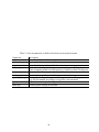
For a better estimate we need to take more measurements. We observed the Sun again at June 30
multiple times. The FWHM was then calculated the same way as above for each measurement.
The results are listed in Table 6. Averaging these values yields a beam size of 12.07 ± 0.13 °.
The error is calculated according to
v
u
t
N
1X
σ=
(xi − x̄)2 .
N
i=1
This is still off from the measured value in the lab. Most likely this is because pointing the telescope such that the sun passes exactly through the middle of the beam is difficult to do, causing
us to measure a smaller FWHM. This may also explain the spread in the values themselves.
40
(a) The signal of the Sun enlarged. In green is the fit for the background.
(b) The Gaussian fit for the main beam (in green).
(c) Indication of the FWHM of the main beam. The value comes down to
11.99°.
41
Table 6: Sun observations June 30
Time (hh:mm:ss)
12:01:32
12:03:18
12:04:58
12:07:01
12:15:58
12:17:53
12:19:52
HPBW (deg)
12.09
12.23
12.08
12.25
11.99
11.92
11.91
42
Error (deg)
0.071
0.073
0.073
0.085
0.082
0.087
0.087
5.4
Measuring the Brightness Temperature of the Sun
If we have calibrated data, we can relate the power from the Sun to a brightness temperature.
This can be determined by calculating the antenna temperature of the Sun. This is most easily
done with the system temperature,
Tsys = TCMB e−τ + Tatm (1 − e−τ ) + Tb, e−τ .
(13)
To determine the brightness temperature we thus need to know the gain of the telescope to
convert the incoming power to a temperature and the optical depth of the atmosphere such
that we can invert the above relation to obtain
Tb, = [Tsys − TCMB e−τ − Tatm (1 − e−τ )]eτ .
(14)
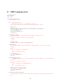
Due to unforeseen complications with the cold load that emerged at the final stages, we unfortunately were not able to correctly calibrate the measurements. Hence it is not possible to
determine the brightness temperature of the sun at this moment.
43
6
6.1
Measurements of other Sources
Galactic Synchrotron Radiation
Electrons in the Milky Way and cosmic ray electrons are accelerated in the magnetic field thus
producing synchrotron radiation. To see if the galaxy’s synchrotron radiation will affect our
measurements we need to know how strong it is with respect to the CMB at 11 GHz. Since
this radiation is frequency dependent we need to know how it scales with ν, which in turn
depends on how the energy is distributed among the electrons. The energy spectrum of cosmic
ray electrons follows a power law relation, giving the energy distribution given by
(15)
N (E)dE ∝ E −δ dE.
This means the brightness temperature will follow the power law given by
(16)
T (ν) ∝ ν −β
with β = (δ+3)/2 being the spectral index for synchrotron radiation. In the range of 1.42−14.9
GHz this spectral index is β = 3.0 [Platania et al., 1998]. The relative intensity of the galactic
synchrotron radiation with respect to the intensity of the CMB is given by
Isync
ICMB
∝ ν β−3 (ehν/kTCMB − 1) [Readhead and Lawrence, 1992].
(17)
I
sync
For a spectral index of 3.0 only the exponential part remains. This results in ICMB
∝ 0.21. This
relation is proportional to, but we can calculate an approximate contribution to the antenna
temperature assuming this ratio and a gain of 60 dB. The power from just the CMB would
be PCMB = −85.03 dBm as seen in chapter 2. If the synchrotron radiation contributes 20%
of this power this changes to PCMBS = −84.19 dBm. This will result in a change of antenna
temperature of ∆TA = 0.046 K. Contribution of synhrotron radiation is therefore most likely
negligible in our case.
6.2
Astrophysical Radio Sources
Besides the Sun the sky houses many other radio sources. I have chosen four sources to investigate: Cassiopeia A, Cygnus A, Taurus A and Virgo A. Cas A is a well known supernova
remnant and is one of the brightest radio sources in the sky. Cygnus A is also a strong radio
source. It is a radio galaxy with two large lobes on either side. Taurus A or the Crab Nebula
is one of the most well known supernova remnants. In it’s center is a pulsar emitting radio
waves. Lastly Virgo A or M87 is an elliptical galaxy with an radio emitting AGN at its center.
Table 8 lists the flux density and the resulting contribution to the antenna temperature of these
sources. The flux densities are calculated according to Baars et al. [1977] who use
log10 S [Jy] = a + b log10 ν [MHz] + c log210 ν [MHz]
(18)
for calculating the flux density of these sources. The parameters for this equation of each source
are listed in Table 7.
44
Source
Cassiopeia A
Cygnus A
Taurus A
Virgo A
a
5.745
7.161
3.915
5.023
b
-0.770
-1.244
-0.299
-0.856
c
0
0
0
0
Table 7: Selected sources with their parameters for the flux density equation.
Source
Cassiopeia A
Cygnus A
Taurus A
Virgo A
Flux Density (Jy)
322.29
135.99
508.89
36.61
Antenna Temperature (K)
0.0054
0.0023
0.0086
0.00062
Table 8: Flux density of the selected sources at 11 GHz and antenna temperature for τ0 = 0.01.
To be able to measure these sources the fluctuations in Data Set HPBW (deg)
Tsys need to be smaller than their respective contribution. 021432
12.27
This means that we need a sensitivity of 0.0086 K or lower 021643
12.48
to detect Taurus A, the brightest of the sources. From the 022009
12.31
available power meter settings we need to use an integra- 025854
12.69
tion time of 0.8 seconds giving a sensitivity of 0.0069 K. 030052
12.78
With an integration time of 1.6 seconds we should be able 030245
12.83
to detect Cassiopeia A with a sensitivity of 0.0049 K. To de- 030443
12.73
tect Cygnus A we need to use the 12.8 second integration 030706
12.57
time to obtain a sensitivity of 0.0017 K. To detect Virgo A 030908
12.66
we need a much longer integration time. The longest in- 031439
12.77
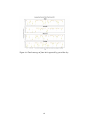
tegration time possible is 51.2 seconds. This gives a sensitivity of 8.6·10−4 K. This is larger than the signal of Virgo Table 9: Measurements containing
A and fluctuations of this order are in the regime of fluc- the satellite and the corresponding
tuations caused by the Allan time. Therefore, we are not HPBW from that dataset.
able to detect this source with our telescope. As for the
other sources, any measurement of the brightness temperature will most likely not possible.
Theoretically it should be possible to make a detection of these sources by making a lot of measurements and then stacking them. This way the noise will be reduced compared to the signal
of the source. However, this is based on the radiometer equation which in our case does not
give the limiting sensitivity. Detection of other sources is therefore most likely not possible.
6.3
Non-Astrophysical Sources
The sky is also home to man made objects such as sattellites. We discovered a sattellite by
accident when trying to find a clear piece of sky. When viewing the data we saw a large peak
that was approximately 3.5 dBm higher than the background. This rules out the Sun as it is much
45
weaker. It is also unlikely to be an astronomical source. The peak is located at 150° meaning
it is 30° above the horizon. Checking the sky for possible sources at this location revealed that
there are geostationary satellites at this location. These satellites are used for communications
and emit high power radio signals. As the satellite is an even stronger point source than the
Figure 24: The mysterious signal. The left peak is the signal from the Sun and the right peak is
from the satellite.
Sun it is an ideal object to check the size of the beam. We use the measurements from June 30
to do this. The results are listed in Table 9. From these measurements we obtain an average
HPBW of 12.61 ± 0.19 °.
46
7
Future Improvements and Conclusion
Performance of the telescope is not yet optimal on the software and measuring side. Possible
points of improvement are:
• Improve the overall speed and efficiency of the code.
• Change the way results are read from the power meter and temperature monitor.
• Use a more powerful motor or implement more advanced motor control.
• Use a more powerful version of the Pi or split the system into multiple components.
7.1
Code Efficiency and Speed
The code to control the telescope is self written. Something that can almost certainly be improved is the code itself. Certain routines can be optimized or special libraries designed for
speed could be used. For even better performance we could switch to a compiled language
such as C instead of Python, an interpreted language. This will however require a complete
rewrite of the control code and it will reduce the flexibility of possible measurements. The performance gain from this switch will not be of great importance either as the other components
in the system become the limiting factors. The code can still be optimized, but it will not give
a significant improvement.
7.2
Reading Results from the Power Meter
The major bottleneck as of now is reading the power from the power meter. Due to the way it
is done now this can take up to a second. This interrupt causes the telescope to wait after each
step instead of moving continuously. Attempts have been made to get around this interrupt
problem by running movement and measurement in parallel. It turned out however that the
CPU on the Pi is not fast enough to handle this. The only way to change this is to use a different
method of reading from the device. There is a specific setup for the GPIB controller and the
power meter that makes it respond as soon as it has something to respond when asked for it.
With this, response times should drop to nearly instantaneously.
7.3
Motor Power and Control
A stepper motor, like any motor, has a maximum load it can drive. Stepper motors in particular
are limited by the amount of torque they can produce. The highest torque is gotten from the
lowest rotation speeds. The faster it spins, the less torque it can generate. This means it might
not be able to start at full speed. More advanced control schemes with, for example, acceleration
towards maximum speed can solve this. A more powerful motor can generate more torque and
would therefore be able to drive the horn at higher speeds right from the start.
Another option would be to implement more advanced control of the motor. The motor
has a recommended operating voltage, but it can endure much higher voltages when moving.
47
Applying a higher voltage gives the motor an increased torque allowing it to start faster. The
downside to this is that higher voltages also induce higher currents and hence increase heat
output. If the motor becomes too hot it can potentially damage or kill it. This can be circumvented by having the voltage gradually increase as the motor gains speed and decrease as it
slows down.
7.4
More Powerful Hardware
The last and most profound changes can be made at hardware level. The Pi is now the main
unit that both controls all devices and processes all signals. To reduce the load on the system
the control could be split up across multiple units. An example would be to use separate units
for moving the motor and for reading the power meter and temperature sensors. These would
then still be controlled from the Pi to coordinate everything, but the load would be spread over
multiple devices allowing for smoother operation.
7.5
Conclusion
During this project I was responsible for control of and acquiring data from the telescope. While
there is still room for improvement, it is in a well usable state for observations. The observations
that I carried out had varying results. The brightness temperature of the Sun could not be
determined due to unforeseen complications, however verifying the beam size was successful
with both the Sun and the satellite. The Sun yields a beam size of 12.07° and the satellite one of
12.61°. The latter is closest to the beam size determined in the lab. This is not surprising since
the satellite was a much stronger source than the Sun.
48
8
Acknowledgements
I would like to thank John McKean for providing this project. It was a great opportunity to
actually apply some of the theory learned in the Radio Astronomy course to a real life problem
of building a radio telescope. My share in this project would not have been possible without all
the help from the electronics department of SRON and the help of other people. I would like to
thank Andrey Barychev, Andrey Kudchenko, Ronald Hesper, Henk Ode and Duc Nguyen for
their help in constructing the electronics, acquiring measurement devices, trouble shooting and
overall help.
49
References
(2012). AstroBaki. Referenced on May 10th, 2015.
Agilent Technologies (2013a). Agilent E4418B Power Meter User’s Guide.
Agilent Technologies (2013b). Programming Guide E4418B/E4419B Power Meters.
Baars, J. W. M., Genzel, R., Pauliny-Toth, I. I. K., and Witzel, A. (1977). The absolute spectrum
of CAS A - an accurate flux density scale and a set of secondary calibrators. AAP, 61:99–106.
Bernard F. Burke, F. G.-S. (2010). An Introduction to Radio Astronomy. Cambridge.
Committee on Radio Astronomy Frequencies (2005). CRAF Handbook for Radio Astronomy.
European Science Foundation, 3 edition.
Ericsson. Industrial circuits application note: Stepper motor basics. Last referenced 10-06-2015.
Fixsen, D. J. (2009). The Temperature of the Cosmic Microwave Background. The Astrophysical
Journal, 707(2):916.
Heraeus (2013). Housed Platinum Resistance Temperature Detector SOT223.
ICS Electronics (2009). IEEE 488 Application Bulletin: GPIB 101 - A Tutorial about the GPIB
Bus.
Jansky, K. G. (1982). 1933, Electrical Disturbances Apparently of Extraterrestrial Origin, page 23.
Article in the book Classics in Radio Astronomy.
Jerri, A. (1977). The shannon sampling theorem #8212;its various extensions and applications:
A tutorial review. Proceedings of the IEEE, 65(11):1565–1596.
J.J. Condon, S. R. Essenstial radio astronomy. Last referenced on 17-05-2015.
KNMI. Data aquisition from a script. Last referenced 06-06-2015.
Lap, B. (2015). Design of a pickett-potter horn to measure the cmb at 11 ghz.
Lee, J. (2007). Radio emissions from solar active regions. Space Science Reviews, 133(1-4):73–102.
Mulder, W. (2015). Calibration of a 11 GHz Pickett-Potter Horn and Measurements of the Cosmic
Microwave Background.
Orientalmotor (2015). Stepper motor basics.
Platania, P., Bensadoun, M., Bersanelli, M., Amici, G. D., Kogut, A., Levin, S., Maino, D., and
Smoot, G. F. (1998). A determination of the spectral index of galactic synchrotron emission
in the 1-10 ghz range. The Astrophysical Journal, 505(2):473.
50
Prologix (2013). GPIB-Ethernet Controller User Manual.
Readhead, A. C. S. and Lawrence, C. R. (1992). Observations of the isotropy of the cosmic
microwave background radiation. Annual Review of Astronomy and Astrophysics, 30(1):653–
703.
Reber, G. (1944). Cosmic Static. Astrophysical Journal, 100:279.
van Schooneveld, C. (1990). Ruis.
Wilson, Kristen Rohlfs, S. H. et al. (2013). Tools of Radio Astronomy. Springer.
Zandvliet, M. (2015). The back-end and mechanics of a pickett-potter horn at 11 ghz.
51
A
Average Temperatures for June
52
Figure 25: Temperatures of June 2007 separated by part of the day.
Figure 26: Temperatures of June 2008 separated by part of the day.
53
Figure 27: Temperatures of June 2009 separated by part of the day.
Figure 28: Temperatures of June 2010 separated by part of the day.
54
Figure 29: Temperatures of June 2011 separated by part of the day.
Figure 30: Temperatures of June 2012 separated by part of the day.
55
Figure 31: Temperatures of June 2013 separated by part of the day.
56
B
Average Cloud Coverage for June
57
Figure 32: Temperatures of June 2007 separated by part of the day.
Figure 33: Cloud coverage of June 2008 separated by part of the day.
58
Figure 34: Cloud coverage of June 2009 separated by part of the day.
Figure 35: Cloud coverage of June 2010 separated by part of the day.
59
Figure 36: Cloud coverage of June 2011 separated by part of the day.
Figure 37: Cloud coverage of June 2012 separated by part of the day.
60
Figure 38: Cloud coverage of June 2013 separated by part of the day.
61
C
Telescope Server
#!/usr/bin/env python
##########################
# Regular Python modules #
##########################
from __future__ import division
import numexpr as ne
import datetime as dt
import errno
import os
import readline
import sys
try:
import RPi.GPIO as GPIO
except RuntimeError:
print ’Error importing GPi.GPIO. Try running as root.’
###########################
# Radio telescope modules #
###########################
import StepperMotor as sm
import GPIBComm as gc
##################################
# Server constants and functions #
##################################
YELLOW_BOX_IP = ’192.168.0.142’
PORT = 1234
label_m
funct_m
label_c
funct_c
=
=
=
=
(’calib’, ’rot’, ’park’, ’prep’, ’turbo’)
(m.calibrate, m.rot, m.park, m.prep, m.set_turbo)
(’measure’, ’speed’, ’speed?’, ’send’, ’unit’)
(c.measure, c.set_measurespeed, c.get_measurespeed, c.send, c.units)
CMD_CTRL = dict(zip(label_c, funct_c))
CMD_MOTR = dict(zip(label_m, funct_m))
def call(func, device, *args):
’’’ Processes the commands given to the server prompt.
Call functions specific to a certain device. Currently available devices are: controller, motor.
Args:
function func - the function to execute.
str device - name string of which type of device to address.
misc args - additional arguments to the function.
Returns:
None
’’’
if device == ’controller’:
if args is not None:
CMD_CTRL[func](*args)
else:
CMD_CTRL[func]()
elif device == ’motor’:
if args is not None:
CMD_MOTR[func](*args)
else:
CMD_MOTR[func]()
else:
print ’Unknown device.’
####################
# Telescope server #
62
####################
# Server startup. Clear the terminal and check if everything is ok.
os.system(’clear’)
print ’=== Kapteyn Radio Telescope Server ===’
try:
# See if the yellow box is alive.
c = gc.GPIB_Controller(YELLOW_BOX_IP, PORT)
c.send(’++ver’)
c.read()
# Ask the power meter to identify itself.
c.send(’++addr 14’); c.read(prnt=False)
c.send(’*idn?’)
c.read()
c.send(’SENS:AVER:COUN:AUTO OFF’)
c.read(prnt=False)
# Aks the temperature monitor to identify itself (it responds by itself).
c.send(’++addr 10’); c.read()
# Default to powermeter.
c.send(’++addr 14’); c.read(prnt=False)
c.units(’dbm’)
except:
print ’An error occured. Is the Raspberry Pi connected to the switch and are the devices turned on?’
sys.exit(-1)
# Initate a motor and calibrate it to zero.
m = sm.StepperMotor(31, 29, 200, 72)
m.calibrate()
# Set up a directory on the users desktop to store measurements in.
try:
os.makedirs(os.path.expanduser(’/home/’+os.environ[’SUDO_USER’]+’/Desktop/’+dt.datetime.now().isoformat()
[:10].replace(’-’, ’’)))
except OSError as e:
if e.errno != errno.EEXIST:
raise
try:
# Enter the main loop.
while 1:
# Ready the input.
inp = raw_input(’>>> ’).lower()
cm = inp.split()
if len(cm) > 1:
cmd = cm[0]
args = cm[1::]
elif len(cm) == 1:
cmd = cm[0]
args = []
else:
cmd = inp
# Process input.
if cmd == ’quit’:
c.quit()
m.quit()
break
elif cmd == ’run’:
# User wants to run his/her own script.
f = args[0]
try:
execfile(’./’+f+’.py’)
except Exception as e:
print e
print ’Failed to execute script’
elif cmd in CMD_CTRL:
63
if len(args) > 0:
call(cmd, ’controller’, *args)
else:
call(cmd, ’controller’)
elif cmd in CMD_MOTR:
if len(args) > 0:
#call(cmd, ’motor’, *[float(a) for a in args ])
call(cmd, ’motor’, *[float(a) if a.strip().isdigit() else a for a in args])
else:
call(cmd, ’motor’)
# Special commands starting with !.
elif cmd.startswith(’!rot’):
m.rot(float(cm[1]), override=True)
elif cmd.startswith(’!calib’):
m.calibrate(override=True)
else:
c.send(inp)
c.read()
except KeyboardInterrupt:
pass
finally:
GPIO.cleanup()
64
D
GPIB Communication
#!/usr/bin/env python
import readline
import socket
class GPIB_Controller(object):
’’’ GPIB_Ethernet Controller.
’’’
def __init__(self, ip, port):
’’’ Initialize a new connection to a GPIB-Ethernet Controller.
Sets up a TCP connection to the controller at the specified ip address and port.
’’’
self.ip = ip
self.port = port
self.sock = socket.socket(socket.AF_INET, socket.SOCK_STREAM, socket.IPPROTO_TCP)
self.sock.connect((ip, port))
self.sock.settimeout(1)
# Initalize to the power meter.
self.addr = 14
def address(self, addr):
’’’ Change the address to the specified value. The address can range from 0 to 30.
Args:
int addr - address of the device to communicate with.
Returns:
None
’’’
self.addr = addr
self.send(’++addr %d\n’ % addr); self.read(prnt=False)
def measure(self):
’’’ Query the power meter to return a measurement. Assumes the address is set to the power meter.
Args:
None
Return:
str res - the answer of the power meter.
OR
None - if the address is wrong.
’’’
self.send(’FETC?\n’)
res = self.read(prnt=False)
return res
def measure_temp(self, sens):
’’’ Query the temperature monitor to return a measurement. Assumes the address is set to the temperature
monitor.
Args:
str sens - the sensor to read out
Returns:
str res - the answer of the temperature monitor.
OR
None - if the address is wrong.
’’’
sensors = {’hot’:1, ’cold’:2, ’atm’:4}
self.send(’KRDG? %d\n’%sensors[sens])
res = self.read(prnt=False)
return res
def read(self, prnt=True, maxiter=2):
’’’ Read responses from the buffer. Keep looping until we receive None to make sure we have the response
.
Args:
65
bool prnt - print the output to the console (default is True).
int maxiter - number of secondary attempts to make when response is None (default is 2).
Returns:
str data or None - response of the GPIB controller.
’’’
data = None
itr = 0
# Keep reading until we have everything.
while (data is None) and (itr < maxiter):
try:
# Query the yellow box to speak to us.
self.sock.send(’++read \r\n’)
# Read from the socket; strip all whitespace (spaces, LF, CR etc.) on the right end.
data = self.sock.recv(4096).rstrip()
except socket.timeout:
# No response or empty lines.
pass
finally:
itr += 1
if prnt:
print data
return data
def send(self, cmd):
’’’ Send a command to the GPIB controller.
Args:
str cmd - command to send.
Returns:
bool True/False - success or failure of sending the command.
’’’
try:
self.sock.sendall(cmd+’\n’)
return True
except:
return False
def set_measurespeed(self, rps=20, avg=1):
’’’ Sets the integration time of the telescope by specifiying the readings per second and the number of
averages taken for a measurement.
Args:
int rps - readings per second. Available: 20, 40 or 200.
int avg - number of averages for a measurement. Available: 1, 2, 4, 8, 16, 32, 64, 128, 256, 512,
1024.
Return:
None
’’’
rp = [20, 40, 200]
av = [2**i for i in range(11)]
rps = int(rps); avg = int(avg)
if (rps not in rp) or (avg not in av):
print ’Invalid value in measure speed.’
return
else:
self.send(’SENS:AVER:COUN %d’ % avg)
self.send(’SENS:SPE %d’ % rps)
def get_measurespeed(self, p=True):
’’’ Requests the averaging rate and readings per second.
Args:
bool p - print the values to the terminal or not.
Returns:
int read - readings per second.
int aver - the number of averages taken for a measurement.
’’’
self.send(’SENS:SPE?’)
66
aver = self.read(prnt=p)
self.send(’SENS:AVER:COUN?’)
read = self.read(prnt=p)
return read, aver
def units(self, un):
’’’ Set the units of measurement. Possible units are ’W’ or ’dBm’.
Args:
str un - unit to return.
Return:
None
’’’
u = un.lower()
if u == ’w’:
self.send(’UNIT:POW W’)
self.read(prnt=False)
elif u == ’dbm’:
self.send(’UNIT:POW DBM’)
self.read(prnt=False)
else:
print ’Invalid unit.’
def quit(self):
’’’ Correctly close the connection to the controller.
Args:
None
Return:
None
’’’
self.sock.close()
if __name__ == ’__main__’:
YELLOW_BOX_IP = ’192.168.0.142’
PORT = 1234
c = GPIB_Controller(YELLOW_BOX_IP, PORT)
c.send(’++ver’)
c.read()
c.send(’*idn?’)
c.read()
while 1:
cm = raw_input(’>>> ’)
if cm == ’quit’:
c.quit()
break
else:
c.send(cm)
c.read()
67
E
Stepper Motor Control
#!/usr/bin/env python
from __future__ import division
import numexpr as ne
import readline
import time
try:
import RPi.GPIO as GPIO
except RuntimeError:
print ’Error importing GPi.GPIO. Try running as root.’
class StepperMotor(object):
’’’ Stepper motor.
’’’
def __init__(self, pdir, pstep, stprev, revdisk):
###############################
# Raspberry Pi GPIO pin setup #
###############################
self.PIN_DIR = pdir
self.PIN_STEP = pstep
# Set pin numbering as on the pi
GPIO.setmode(GPIO.BOARD)
# Set pins as output pins.
GPIO.setup(pdir, GPIO.OUT)
GPIO.setup(pstep, GPIO.OUT)
####################
# Motor constants #
####################
self.REV_DISK = revdisk
disk revolution.
self.STEP_STPM = stprev
self.STEP_DISK = self.STEP_STPM * self.REV_DISK
self.SLEEP_TIME = 0.002
self.TURBO = False
self.PARK_POS = 0
self.ANGLE = 0
self.CALIBRATED = False
self._rotating = False
# Number of stepper revolutions required for one
#
#
#
#
#
#
#
Number of steps per stepper motor revolution.
Number of steps per disk revolution.
Number of seconds to sleep between steps.
Shorter sleep time hence faster movement.
Parking position.
Tracks telescope position.
Check for calibration.
def calibrate(self, override=False):
’’’ Calibrate the telescope to the parking posistion.
Args:
float cal_ang - set the current angle to the parking angle.
bool override - override the existing calibration.
Returns:
None
’’’
if (not self.CALIBRATED) or (self.CALIBRATED and override):
# Set the current angle to this position.
self.ANGLE = 0
self.CALIBRATED = True
else:
print ’System already calibrated.’
@property
def is_rotating(self):
’’’ Returns wether the motor is rotating or not.
’’’
return self._rotating
68
def park(self):
’’’ Return the telescope to park position.
Args:
None
Returns:
None
’’’
self.rot(-self.ANGLE)
def prep(self):
’’’ Prepare the telescope for calibration starting from zero point.
This points the horn to the cold load at -15 degrees from the horizontal.
Args:
None
Returns:
None
’’’
self.rot(-15, override=True)
def rot(self, ang, override=False):
’’’ Rotate the disk by a given amount of degrees.
There are built in safety limits so that the telescope will not move below 0 or over 180 degrees. This
protection should not be overridden unless you know what you are doing. In general it should not be
necesarry to do this.
Args:
float ang - rotation angle in degrees.
bool override - override the safety limits. Use carefully!
Return:
None
’’’
self._rotating = True
# Update the telescope position.
if (((self.ANGLE + ang) > 180) or ((self.ANGLE + ang) < 0)) and not override:
print ’Going too far! Aborting.’
return
self.ANGLE += ang
# Set forwards or backwards.
if ang < 0:
self.set_direction(True)
else:
self.set_direction(False)
# Calculate the number teps needed.
steps = (abs(ang) / 360) * self.STEP_DISK
istep = 0
while istep < steps:
self.step()
istep += 1
self._rotating = False
def set_direction(self, direction):
’’’ Set the movement forwards or backwards.
Args:
bool direction - True: backwards, False: forwards.
Return:
None
’’’
GPIO.output(self.PIN_DIR, direction)
def set_turbo(self, x):
’’’ Change the delay between switching pin states.
If turbo is on the torque produced by the motor will be lower.
Args:
69
int x - 0 or 1 for turbo on or off.
Return:
None
’’’
if x:
#self.TURBO = True
self.SLEEP_TIME = 0.0013
else:
#self.TURBO = False
self.SLEEP_TIME = 0.002
def step(self):
’’’ Make the stepper motor do one step.
Sleep occurs _after_ state change. This means the following cycle: high, sleep, low, sleep. This means
movement is slower by a factor of two w.r.t to the sleep time.
Args:
None
Return:
None
’’’
GPIO.output(self.PIN_STEP, True)
time.sleep(self.SLEEP_TIME)
GPIO.output(self.PIN_STEP, False)
time.sleep(self.SLEEP_TIME)
def quit(self):
’’’ Properly exit the motor controls.
Args:
None
Return:
None
’’’
GPIO.cleanup()
if __name__ == ’__main__’:
mot = StepperMotor(38, 40, 200, 72)
while True:
cmd = raw_input(’>>> ’).lower()
com = cmd.split(’ ’)
if len(com) == 2:
command = com[0].lower()
arg = com[1]
if command == ’rot’:
deg = ne.evaluate(arg)
mot.rot(deg)
if command == ’!rot’:
deg = ne.evaluate(arg)
mot.rot(deg, override=True)
elif cmd == ’calib’:
mot.calibrate()
elif cmd == ’!calib’:
mot.calibrate(override=True)
elif cmd == ’park’:
mot.park()
elif cmd == ’quit’:
break
else:
print ’Invalid command.’
GPIO.cleanup()
70
F
DNS Configuration
# Set up for the ethernet port of the Pi.
interface=eth0
# Give out IP addresses betweeon 0 and 100 with 1 hour lease time.
dhcp-range=192.168.0.20,192.168.0.100,255.255.255.0,1h
# Logs
log-facility=/var/log/dnsmasq.log
log-async
log-dhcp
71