Download "user manual"

ABSTRACT
This thesis reasons on dynamic wireless sensor networks (WSN) analyzing
different models and architectures. The main goal of all the work is the
development of a tool designed to fulfill the needs of real on-field research,
especially applied to indoor environment such as houses and hospitals. The
idea was born from my last university thesis where alongside the original
project of a remote controlled surgical room arose the need to monitor the
hospital's patients and surgeons. In that occasion we were forced, for many
reasons, to use a sort of batch system consisting of RFID tags and sensors
with memory, whose data were downloaded after many hours or days, or
simply sensors directly connected to computers. Instead a set of wireless
sensors have allowed a real-time interaction with the remote controlled
system.
My thesis first shows a background of the wireless sensor network theory,
technologies and security issues and shows how the work was developed.
In the first period of time a developer starter kit was chosen from many
available, evaluating different properties, including costs, open source or
free IDE and the possibility of modify the base library supplied.
An initial project was developed using this kit, modifying the nodes to
install the required sensors. Following the main requests of the team, the
network was created balancing the energy consumption and the reliability.
The developing work was supported by field tests on real research scenarios
of increasing complexity. The initial test results on the original project,
developed with the supplied library, revealed weaknesses in battery life,
nodes connection stability and security thus changes were made
accordingly. An heartbeat system was designed and implemented to create a
fault tolerant system consisting in a couple of devices. Then the security
issues were evaluated in consideration of the increasing number of attack's
techniques designed for the WSNs. A cryptography key protection
mechanism was implemented to protect the AES algorithm itself and the
data, together with a software deletion mechanism, in front of an hardware
read access, to avoid the steal of the initial pass-phrases of the program
itself. Finally some consideration were made on the WSN performance and
study results. In conclusion we can say that our wireless network has been
used successfully, although it has shown limits on stability and data flow
capacity. In most cases the WSN capacity of disappearing and to be
unattended for long time were preferred then the data stream reliability
because of the comfort quality perceived by study’s subjects (i.e. house's
inhabitants or patients).
1
to my beloved Samuela
and all my family
3
4
Contents
ABSTRACT .................................................................................................. 1
CONTENTS.................................................................................................. 5
1
2
INTRODUCTION.............................................................................. 11
1.1
THE STATEMENT ........................................................................... 11
1.2
MOTIVATIONS ............................................................................... 12
1.3
STUDY CONTEXT ........................................................................... 13
1.4
PROBLEMS AND CHALLENGES ....................................................... 14
1.5
THE APPROACH ............................................................................. 15
1.6
ORGANIZATION OF THE THESIS ...................................................... 16
WSN APPLICATIONS ..................................................................... 19
2.1
APPLICATION DOMAINS ................................................................. 19
2.1.1
Industrial control and monitoring............................................ 19
2.1.2
Home automation and consumer electronics........................... 20
2.1.3
Security and military sensing ................................................... 21
2.1.4
Asset tracking and supply chain management ......................... 22
2.1.5
Intelligent agriculture and environmental sensing .................. 23
2.1.6
Health monitoring .................................................................... 23
2.2
NETWORK PERFORMANCE OBJECTIVE ........................................... 25
2.2.1
Low power consumption .......................................................... 25
2.2.2
Low cost ................................................................................... 25
2.2.3
Security..................................................................................... 26
2.2.4
Network type............................................................................. 28
2.2.5
Worldwide availability ............................................................. 28
5
2.2.6
Data throughput ....................................................................... 28
2.2.7
Message latency ....................................................................... 29
2.2.8
Mobility .................................................................................... 29
2.2.9
Size ........................................................................................... 29
2.3
3
WSN CLASSIFICATION AND STANDARDS .............................. 33
3.1
A DEFINITION OF WSN.................................................................. 33
3.2
WSN CLASSIFICATIONS ................................................................. 35
3.2.1
Single-sink single-hop WSN ..................................................... 36
3.2.2
Single-sink multi-hop WSN ...................................................... 37
3.2.3
Multi-sink multi-hop WSN........................................................ 37
3.2.4
Actuators .................................................................................. 39
3.3
3.3.1
3.4
WIRELESS SENSOR NETWORK STANDARDS .................................... 40
The IEEE 802.15.4 low-rate wpan standard............................ 41
PROTOCOL LAYERS ....................................................................... 46
3.4.1
The physical (PHY) layer ......................................................... 46
3.4.2
Packet structure ....................................................................... 50
3.5
THE MEDIUM ACCESS CONTROL (MAC) LAYER ............................. 50
3.5.1
Frame and super-frame structure ............................................ 54
3.5.2
The association request and response command formats........ 59
3.5.3
The Disassociation Notification............................................... 60
3.5.4
Security..................................................................................... 61
3.6
4
WSN APPLICATION TAXONOMY .................................................... 31
ZIGBEE STANDARD ....................................................................... 62
3.6.1
The network layer (NWK APL) ................................................ 62
3.6.2
The application layer ............................................................... 65
3.6.3
ZigBee Versions from 2004 to PRO ......................................... 65
3.6.4
Brief comparison with other protocols .................................... 67
WSN IMPLEMENTATION ASPECTS .......................................... 71
6
4.1
NETWORK FORMATION AND ADDRESS ASSIGNMENT FOR A
HIERARCHICAL (TREE) TOPOLOGY ............................................................ 71
4.1.1
4.2
ROUTING ALGORITHMS FOR A MESH TOPOLOGY ............................ 77
4.2.1
Dynamic source routing........................................................... 78
4.2.2
On-demand distant vector ........................................................ 79
4.2.3
Zigbee Route discovery ............................................................ 79
4.2.4
Route discovery ........................................................................ 84
4.2.5
Route maintenance and repair ................................................. 90
4.3
THE NWK LAYER MANAGEMENT SERVICE .................................... 91
4.3.1
Network discovery.................................................................... 91
4.3.2
Network formation ................................................................... 92
4.3.3
Establishing the device as a ZigBee router.............................. 92
4.3.4
Joining and leaving a network ................................................. 93
4.3.5
Resetting the NWK layer .......................................................... 95
4.3.6
Synchronization........................................................................ 96
4.3.7
The NWK layer frame formats ................................................. 97
4.4
THE APL LAYER ......................................................................... 102
4.4.1
The application framework .................................................... 103
4.4.2
The ZigBee device objects...................................................... 109
4.4.3
The APS sublayer ................................................................... 112
4.5
5
Routing in ZigBee tree topology .............................................. 76
SECURITY .................................................................................... 114
DESIGN AND IMPLEMENTATION OF A WSN....................... 117
5.1
SELECTION OF THE DEVELOPER KITS ........................................... 117
5.2
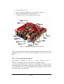
MESHNETICS STARTER KIT .......................................................... 118
5.2.1
Hardware general specification............................................. 120
5.2.2
MeshBean2’s expansion connectors ...................................... 120
5.2.3
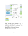
eZeeNet functional diagram................................................... 121
5.2.4
EZeeNet API........................................................................... 124
7
5.2.5
5.3
DEVELOPMENT OF APPLICATION CODE ........................................ 125
5.3.1
General Software Specification and user code limitations .... 126
5.3.2
TinyOS Functions................................................................... 127
5.3.3
Framework Interfaces ............................................................ 129
5.4
DEVELOPMENT OF THE APPLICATION .......................................... 130
5.4.1
Call Sequences ....................................................................... 139
5.4.2
The heartbeat system.............................................................. 145
5.5
BUFFERING.................................................................................. 148
5.6
DATA COMPRESSION ................................................................... 149
5.6.1
Data structure ........................................................................ 150
5.6.2
Data compression validation ................................................. 152
5.6.3
Compression results ............................................................... 153
5.6.4
The software analysis............................................................. 154
5.7
6
State after reset ...................................................................... 125
PRACTICAL OF EXPERIENCES ON MESHNETICS BOARDS .............. 158
5.7.1
The hardware analysis ........................................................... 159
5.7.2
Board changes and additions................................................. 161
5.7.3
Extracting Keys from Second Generation Zigbee Chips........ 163
RESULTS ......................................................................................... 169
6.1
6.1.1
6.2
WSN PERFORMANCE BENCHMARKS ............................................ 169
Application performance........................................................ 170
ON-FIELD TEST APPLICATION I .................................................... 176
6.2.1
The monitoring system ........................................................... 179
6.2.2
Data analysis.......................................................................... 187
6.2.3
The efficiency of the HVAC heat exchanger. ......................... 189
6.2.4
Conclusion of the first on-field study ..................................... 190
6.3
ON-FIELD TEST APPLICATION II................................................... 190
6.3.1
The monitoring system ........................................................... 192
6.3.2
Conclusion of the second on-field study................................ 193
8
6.4
7
THE NETWORK INTRUSION DETECTION SYSTEM (NIDS) ............. 194
CONCLUSIONS AND FUTURE WORKS ................................... 197
7.1
EVALUATION OF RESULTS ........................................................... 197
7.2
DIFFICULTIES ENCOUNTERED ...................................................... 200
7.3
PERSPECTIVES ............................................................................. 201
7.3.1
7.4
MCU Evolution (the third generation devices)...................... 202
OPEN PROBLEMS ......................................................................... 203
BIBLIOGRAPHY .................................................................................... 205
A.
SECURITY ATTACKS AND ATTACKERS ........................... 215
B.
DEVELOPMENT KITS AND MESHNETICS ‘HOW TO’
GUIDE....................................................................................................... 229
C.
DATA COMPRESSION.............................................................. 245
D.
ACRONYMS ................................................................................ 251
ACKNOWLEDGEMENTS..................................................................... 255
9
1
Introduction
1.1 The statement
The wireless sensor networks are rapidly evolving in these years attracting
interest in a number of application domains related with monitoring and
control of phenomena, as they promise to accomplish tasks at low cost and
with ease.
Researchers see WSNs as an “exciting emerging domain of deeply
networked systems of low-power wireless motes with a tiny amount of CPU
and memory, and large federated networks for high-resolution sensing of the
environment” [WMC04].
In a WSN, the sensors have a variety of functions, and capabilities. The
research’s field is now going forward under the push of recent technological
advances and the pull of a plethora of potential applications.
Most of the actual sensor’s networks as the radars system, nation weather
stations, country electrical power grid are all examples of sensor’s networks;
however all these systems use specialized computers and communication
protocols and consequently, are very expensive.
Much cheaper WSNs are now being developed for coming applications in
security, health-care, and commerce. These systems are multidisciplinary
and involves radio signals and networking, signal processing, systems
architectures, database management, resource optimization, power
management algorithms, and platform technology such as operating
systems.
The networking principles and protocols of these systems are relatively
young and are being developed in these years [KEW02].
The recent engineering advances coupled with many other factors as
ubiquity of the Internet or the developments in IT, are opening the door to a
new generation of low-cost sensors that are capable of achieving high-grade
spatial and temporal resolution.
However there are many difficulties in application development that slow
down the adoption of WSN technology.
11
In most cases the developers need to focus at hardware level to solve
problems, requiring a very close knowledge of the operating system used
beyond physical architecture.
According to [Mot06] the technical background needed is seldom found in
high level domain experts and, as a second problem, the programmer
usually loses the general view and application logic.
To simplify the developing without sacrifice the efficiency, a high-level
abstraction is needed and several different solutions and approaches have
been proposed.
In this thesis we study the development of a WSN, evaluating different
approaches and techniques, building a complete system useful in real onfield researches.
1.2 Motivations
The main goal of this work is the development of a tool designed to fulfill
the needs of real on-field research, especially applied to indoor environment
such as houses and hospitals.
The idea of this study of such a WSN system arose during my master degree
thesis [Gad06]. In that project study , started on 2003, we developed a
prototype of a real-time control system of surgical theatres data flows.
While we did not find any particular problem gathering data from the
surgical room programmable logic controller (PLC) and studying a possible
evolution of such PLC, many problems were found trying to analyze the
incoming data from patients and medical staff.
These human data are very valuable to estimate the infections (literature
estimate the patient’s infection probability at more than 40%, with the 10%
of the total with critical infection such as septicemia, (see [Sco09]) or
hypothermia risks (even more dangerous than infections due to its direct
implications to death) of the patient.
It is to underline that each critical infection, as an example, in the 2009
American implications infections cost report are declared to have a mean
cost of over 13 thousands dollars [Sco09].
On the other hand the medical staff comfort, mainly the surgeons, is very
important to reduce staff errors probability, especially in surgery requiring
several hours.
In that study we were forced to use a sort of batch system consisting of
RFID tags, sensors with their own memory and battery (iButton), whose
data were downloaded after many hours or days, or simply sensors directly
12
connected to computers. Instead a set of wireless sensors have allowed a
real-time interaction with the remote controlled system.
The main reasons for such solution were the availability on the market of
only ad-hoc systems with proprietary firmware that were designed to fit one
specific problem and usually with an high cost. For instance the Bluetooth
kit used in [FGM08], (kindly granted for a period from manufacturer at no
cost) as a price of some thousands Euro and has all the typical problems of
the Bluetooth devices: the modules cannot be used simultaneously due to
their Bluetooth configuration and highly suffer the proximity of other
Bluetooth devices (e.g. mobile phone often in the pocket of medical staff
even when in a surgical room), moreover cannot cover areas greater than
few meters (about 10m).
Moreover the Wireless Sensor Networks (WSNs) such as the ZigBee were,
at time of the beginning of my master degree thesis, just at its first
generation devices (a radio device without logic needing a separate MCU to
perform most of the operations), and where considered more a new study
field rather than a support to other projects.
If can be designed a WSN, capable of different kind of measurements,
without interfering with the common patients and medical staff behaviors, it
can be very useful to cover a wide range of applications allowing the
monitoring, even for long periods, of the environments and their living
peoples while they are performing everyday operations.
Finally we can say that literature lacks in these type of studies in many
fields in which, instead, they can help to support or refute a theory.
1.3 Study context
My work was developed at CIAS (Centro Ricerche Inquinamento ambienti
Alta Sterilità - pollution of high sterility environment research center) a
interdepartmental research centre directed by professor S. Mazzacane and
collaborating with different kind of scientists such as engineers, biologists,
medical staff, IT staff, architects and sometimes physicists.
The centre cover many different areas starting with high sterility
environments, such as cleanrooms, and indoor air quality (IAQ), including
thermo-hygrometric and olfactory parameters, to reach issues related to
mental or physical diseases. Sometimes two different areas converge into a
unique research scenario such as in [Gad06] where the pollution and dust
presence in a surgical room (a high sterility environment) controlled by our
system prototype can be correlated to the patients’ infections.
13
The system design, of course, must be aware of this different application
scenarios and needs.
1.4 Problems and challenges
As the project context suggest (see par. 1.3) the system must be designed to
adapt to different situations, it needs to be easily divided into many
networks if there are many concurrent studies or subjects to analyze. Thus,
in our case, it is not suitable a special device that acts as a gateway from the
WSN to a computer, but is much more useful that many devices can
perform such a role. The second need of our system is the flexibility which
means that we can easily:
•
•
•
change the type of sensors, and this operation can be performed by
any researcher. This problem involves both the hardware design, that
can require modifications and the software development, for
example building a modular sensors driver library
change the way the nodes act in the network can be modified
accordingly to their kind of activity (i.e. continuous measurements
sampling or long idle periods). For this properties the application
design must be as dynamic and event/environment driven as
possible.
place the nodes (or the sensors only) in hostile environments such as
wet pipes or unattended locations. Usually we can achieve this goal
protecting the node and choosing the sensors wisely.
The main features of the projected solution must be the non interference
with the living people, this is of great relevance when trying to convince the
potential subject’s of study, as well as the possibility to monitor and interact
with the system remotely, required not only by the cooperating research
centre but also to achieve the non-interference task.
One of the main challenges, instead, come from the device energy
consumption, since it can greatly affect the period of time the WSN can
achieve its task without an external (and invasive) intervention.
Another challenge is the WSN coordinator bottleneck. In fact all network
topologies where a central node exist where most of the traffic (in our case
the data flow) needs to pass through, then this node will be a bottleneck. In
WSNs this node is the gateway device (the WSN coordinator) that connects
the WSN to other networks or to just a single computer.
14
Finally we must consider the node firmware, growing in size each time a
new specifications set is released, taking the most part of the
microcontroller memory (and sometimes computing) resources.
1.5 The approach
We start considering the WSN as part of a system to automatically gather
data. The system required must be used in an inhabited environments with
the less impact possible, avoiding any kind of discomfort to the living
people.
We have studied the taxonomy of our researches and identified the
minimum requirements to satisfy. This system must be flexible to adapt at
many different contexts having the ability to change from a space time
properties of type local/periodic (such as HVAC monitoring) to a much
more intensive application global/event driven (such as environment
condition or people action control-response).
Apart from the environment’s impact, the development time is also
considered a crucial aspect, since most researches cannot wait months to
start gathering data because of a software problem, most of the times,
indeed, even a manual intervention is preferred to an automatic system non
really reliable and inefficient.
We have started from the WSN state of the art [BPC07] to evaluate the best
solution to fit our WSN system, we have chosen the ZigBee WSN as a large
recognized emerging standard with several manufacturer proposals and we
have used one of this proposal to develop our system.
We have finally used our studies as a test-bed field to prove how really
efficient and flexible is the WSN system. To achieve the task of sensor
interchangeability we have designed a modular library that can be reduced
(with only a sensors driver selection) for memory requirements. In this way
the nodes can be configured by a command sent via the WSN coordinator
without the need to change the node firmware itself but just needing a warm
reset (usually the reset request is also sent via the coordinator device).
We have partially redesigned the upper layer (the Network layer) to solve
some communication problems such as isolated nodes, timer malfunctions
and to dynamically change the node role inside the network. To add more
reliability to the application we have also implemented an heartbeat system,
that is not a new idea, but is adapted to a wireless context using the beacons
of the first device as the beat signals and, moreover, saving the battery
energy of the second node.
15
On the test results basis we have, also, improved the WSN reliability and
security covering the weakness found, such has the possibility to read the
AES key from the node memory or the flaw against DOS attack exploiting
the AES-CTR procedure.
Moreover a Network Intrusion Detection System (NIDS) was modified to
use a special WSN node (a network sniffer) and a packet capture library to
gather and monitor ZigBee network traffic.
Finally to improve the WSN performance we have implemented a Huffman
compression algorithm (only the compression with a static table on the
node) due to its simplicity and compression speed, this partially solve the
bottleneck problem when we have a single sensor (e.g. an tri-axial
accelerometer) producing an high data flow (90 values/sec or more), but the
WSN can also be split into many networks since each node can act as the
coordinator.
Part of the system design effort has been directed to the applications
projected to gather the data from the WSN, send the data to the database
server. For performance and memory reasons the application is
multithreaded (and can be executed without problems on a Pentium III PC).
Furthermore a web interface was created to allow the scientists’ remote
access. This actual system shows the data with a delay of few seconds
(typically less than 2 seconds) thus, for the kind of requirements we have, it
can be considered a real-time system.
1.6 Organization of the thesis
Apart from this introduction the following chapter propose an overview of
the Wireless Sensor Networks. In the third chapter are shown the WSN
classification, standards, and protocol layers.
Next are proposed some WSN implementation aspects used while
developing the application such as network formation, routing algorithms
and security issues. It’s also includes some of the ZigBee higher layers
because of their been both accessed and modified during the application
developing.
The fifth chapter aims to describe the author work done starting from the
choice of the devices and their hardware modifications, to the completion of
WSN application.
The subsequent chapter is dedicated to the results achieved by our WSN
system, thus are described the benchmark, throughput and lifetime results
obtained and the on field test applications with their relative gateway
applications.
16
Finally in the last chapter were presented the author’s conclusions and
perspectives for the future works.
17
2
WSN Applications
2.1 Application domains
We can briefly see the main application domains for the WSN as described
in [Cal06]. The environment can be the physical world, a biological system,
or an information technology (IT) framework. And new doors are opening
everyday as a result of the technology improvements.
We must not forget that a stated goal is to develop complete MEMSs–based
sensor (micro-electro-mechanical systems) at a volume of 1 mm3
[WMC04].
2.1.1 Industrial control and monitoring
A industrial facility has a relatively small control room, surrounded by a
large plant. The control room has usually several indicators and displays
that describe the state of the plant (valves, quantity, temperature and
pressure of stored materials, equipment’s condition, and others) and input
devices that control actuators in the plant (heaters, valves, etc.) that affect
the state of the plant itself.
The sensors, their displays, the input devices and the actuators are often
relatively inexpensive compared with the cost of the armored cable that
must be used to communicate in a wired installation.. The information
shown usually changes slowly so the data bandwidth required is relatively
small although a high reliability level is required.
The costs can be significantly reduced if an inexpensive wireless
communication is used instead and a multiple routing network can be used
to maintain the reliability level.
An example of wireless application in an industrial environment [Cal06]
is the control of commercial lighting. A wireless system can be programmed
to control the lights, grouping them with ease to turn on and off
simultaneously, cutting down the expense of all wired switch and can be
much more flexible when a change is needed.
19
The monitoring and control of moving machinery, where wired sensors and
actuators are often unusable, is another area suitable for wireless networks.
Because the wireless networks may implement distributed routing
algorithms and can be self-healing they can proof to be resilient to an
explosion or other serious damage to the industrial plant, providing officials
with critical plant status information under difficult conditions.
To accomplish to such a job it is important that the wireless system be fully
operating for the entire interval between maintenance periods.
This implies, among others the use of a wireless sensor network with very
low energy requirements.
The sensor node often must be small, inexpensive and easy to substitute.
Wireless sensor networks may be of particular use in the prediction of
component failure for aircraft, where these attributes may be used to
particular advantage [Fri01].
Another application in this area for wireless sensor networks is the heating,
ventilating, and air conditioning (HVAC) of buildings.
This is one of the application also of the WSN developed during my thesis
period.
HVAC systems are typically controlled by a small number of thermostats
and humidistat strategically located. Once more the wired connections limit
the possibility and the number of these thermostats and humidistat
To improve the granularity response of a HVAC system wireless handlers
and dampers can be used coupled with wireless thermostats and humidistat
sensors that may be placed around each room to provide detailed
information about the control system. So the HVAC system can fit the need
of the working team, for example reducing the volume dampers for an
empty project-room and opening dampers for the meeting-room while in
use. A wired system usually lacks to accomplish such a task.
2.1.2 Home automation and consumer electronics
There are many possible applications for wireless sensor networks at home.
[Cal02]. Many of the industrial applications, someone described in the
previous paragraph, may be used in a home, for example a HVAC system
exist, and equipped with wireless thermostats, dampers and the right sensors
can keep the rooms of the house comfortable in a way more efficient than a
home equipped with a single and wired thermostat.
However, a lot of other opportunities are available, like the “universal”
remote control, typically a PDA (personal digital assistant) device that can
control not only the TV, CD player, but the lights, any kind of curtains,
locks that are also equipped with a wireless sensor network connection.
20
With this remote control, one may control the house from the comfort of
one's armchair.
One of the most interesting application, however, comes from the
combination of multiple services, such as closing the curtains automatically
when the television is turned on, or automatically muting the entertainment
system when a call is received on the telephone.
Another application in the home is a sensor-based information appliances
that transparently interact and work together as well as with the home
occupant [Pet00]. These networks are an extension of the information
appliances proposed by Norman [Nit06].
Toys represent a large market for wireless sensor networks, they can be
enhanced or enabled by wireless sensor networks in several ways, limited
only by one's imagination.
A particularly interesting field is PC-enhanced toys, which use the
computing power of a nearby computer to add functionality to the toy itself,
for example, speech recognition and synthesis, without placing the
expensive yet limited speech recognition and synthesis circuits in the toy but
using the computing power of the computer. The overall cost of the toy will
be reduced improving its capabilities and performance.
It is even possible to give the toy complex behavior not practical with other
technologies (see http://toys.media.mit.edu/).
Another home application is similar to the Remote Keyless Entry (RKE)
feature found on many cars. With a WSN, wireless locks, door and window
sensors, and wireless light controls, the home owner may have a remote
control similar to a car-key with a button. When the button is pressed, the
device locks all the doors and windows in the home, and additionally can
turns off the programmed indoor lights, turns on outdoor security lights, and
sets the home's HVAC system to nighttime mode.
The user receives an ok sound once this is all done successfully or an error
code if something goes wrong and in this case he can read on the display
where is the source of the problem. Also a full home security system can be
implemented as well to detect a broken window or other troubles.
Outside of the home, the wireless sensor networks are suitable for many of
activities consumer-related, like tourism and shopping [ACK94].
In these contexts WSNs can provide, furthermore, specific information
about the consumer’s behaviors .
2.1.3 Security and military sensing
The security system described in the previous paragraph for the home
environment can be use in industrial security applications.
21
Similar systems have existed for several years [Swa96] employing
proprietary communication protocols.
They can support multiple sensors relevant to security, including magnetic
door opening, infrared, broken glass sensors, smoke and sensors for direct
human intervention.
One of the benefits of using wireless sensor networks is that they can be
used to replace guards and sentries, not only in military field, around
defensive perimeters.
In addition wireless sensor networks can be used to locate and identify
targets for potential attack or to support the attack by locating friendly or
enemy troops and vehicles.
Wireless sensor networks can be camouflaged to look like rocks, trees, or
gravel. These networks, are difficult to destroy in battle, thanks to their
distributed control and routing algorithms [Hew01].
The use of spread spectrum techniques, combined with the burst
transmission format, common to many wireless sensor networks (to
optimize battery life), can give them a low probability of detection by
electronic means.
2.1.4 Asset tracking and supply chain management
A lot of application of wireless sensor networks is expected to be
concerning resource tracking and supply chain management.
One example is the tracking of containers in a port. Such port facilities may
have thousands of containers or even more, some of which are empty,
while others are to be shipped in different destinations and they are stacked,
on land and on ships.
The efficiency of organization is an important factor in the shipper's
productivity so that they can be moved the fewest number of times and with
the fewest errors. [Cal06]
An error in the location record of any container can be very expensive and
the lost container can usually only be found by an exhaustive search.
Wireless sensor networks can be used to improve such required efficiency;
by placing sensors on each container, its location can always be determined.
Similar problems can be found in railways transport system where railroad
cars of different types must be organized, and in the industries of nondurable goods.
The use of wireless sensor networks for the tracking of nuclear materials has
already been demonstrated in the Authenticated Tracking and Monitoring
System (ATMS) [Sch98], [Sch00].
The ATMS profit from wireless sensors (state of the door, infrared, smoke,
radiation, and temperature sensors) within a shipping container to monitor
22
the state of its contents. Notification of events are transmitted within the
shipping container via a wireless system to a mobile processing unit
connected to a GPS receiver and an International Maritime Satellite
(INMARSAT) transceiver. Through the INMARSAT system, the location is
well known and so is the status of each shipment which may be monitored
anywhere in the world.
2.1.5 Intelligent agriculture and environmental sensing
An example of the use of wireless sensor networks in agriculture is the
rainfall measurement. Large farms and ranches may cover several square
kilometers, and they may receive rain only occasionally and only on some
portions of the farm. Thus it is important to know which fields have
received rain, so that irrigation, usually expensive, can be omitted and
which fields have not and must be irrigated.
Such an application is ideal for wireless sensor networks. The amount of
data sent over the network is usually very low (if is of type "yes or no rain"
is just of one bit), and the message latency can be on the order of several
minutes. However costs must be low and energy consumption must be low
enough for the entire network to last an entire season.
The wireless sensor network is capable of much more than just rain soil
measurements because the network can be fitted with a large variety of
chemical and biological sensors.
This type of application is very important in vineyards, where
environmental changes may have vexing effects on the value of the final
product.
The location determination features of wireless sensor networks may be
used in advanced control systems to enable more automation of farming
equipment or in the determination of animals’ position.
Wireless sensor networks may also be used for low-power sensing of
environmental contaminants such as mercury [Bri98].
MEMS sensors may be integrated with a wireless transceiver in a standard
CMOS process, providing a very low-cost solution to the monitoring of
chemical and biological agents.
2.1.6 Health monitoring
“Health monitoring” is usually defined as “monitoring of non-life-critical
health information”, to differentiate it from medical telemetry, and in this
field wireless sensor networks is expected to grow quickly, although WSN
can applied to some telemetry application as well.
23
We can classify health monitoring applications into two general classes
available for wireless sensor networks. The first class is athletic
performance monitoring, for example, tracking one's pulse and respiration
rate via wearable sensors and sending the information to a personal
computer for data analysis [Ber01]. The second class is at-home health
monitoring like personal weight management [Par00].
The patient's data can be wirelessly sent to a personal computer and then be
used, analyzed or just saved. Another example is the remote monitoring of
patients with chronic disorders like diabetics [Lub02].
The use of wireless sensor networks in health monitoring is expected to
increase rapidly due to the development of biological sensors compatible
with conventional CMOS integrated circuit processes [YLH02].
The sensors, which can detect nucleic acids, enzymes, and other biologically
materials, can be very small, enabling their applications in pharmaceuticals
and medical care.
A developing field market is that of implanted medical devices. In the USA,
the Federal Communications Commission (FCC) established rules
governing the Medical Implant Communications Service, "for transmitting
data in support of diagnostic or therapeutic functions associated with
implanted medical devices." (see http://wireless.fcc.gov).
A developing field related not only to health monitoring is that of disaster
relief. For example, the wireless sensors of the HVAC system in a collapsed
building (earthquake event or gas explosion) can provide victim location
information to rescue workers if acoustic sensors, activated automatically by
accelerometers or manually by emergency personnel, are included.
Wireless disaster relief systems like avalanche rescue beacons, which
continuously transmit signals, are already on the market, so that rescuers can
use to locate the wearer while is in an emergency situation, are used by
skiers and other mountaineers in avalanche-prone areas.
The actual systems have their limitations, first of all they provide only
location information, and give no information about the health of the
wearer. Thus in a large avalanche, when several beacons can be detected by
emergency personnel, There is no way to decide who should be assisted
first.
It was recently proposed that these systems be enhanced by the addition of
health sensors, including oximeters and thermometers, so that would-be
rescuers would be able to identify those still alive under the snow [Mic02].
24
2.2 Network performance objective
To meet the requirements of the applications just described, a wireless
sensor network design must achieve several objectives. The need for these
features leads to a combination of technical issues not found in other
wireless networks.
2.2.1 Low power consumption
WSN applications usually require network components with a power
consumption that is lower than currently required by implementations of
existing wireless networks such as Bluetooth.
For example, devices for certain types of smart tags, badges, or medical
sensors powered from small coin cell batteries, should last for several
months or even years.
The monitoring and control applications of industrial equipment require
exceptionally long battery life so that the maintenance schedules of the
monitored equipment are not compromised. Other applications may require
a very large number of devices that make frequent battery replacement
impractical.
Moreover there are applications that cannot employ a battery at all; network
nodes in these applications must get their energy from the environment
[Sta99]. An example may be the wireless car tire pressure sensor, for which
it is desirable to obtain energy from the mechanical or, as alternative,
thermal energy present in the tire instead of a battery that may need to be
replaced before the tire does [Cal06].
In addition to low power consumption a system with limited power sourcing
often has limited peak power sourcing capabilities as well and this is an
important factor to consider in system design.
2.2.2 Low cost
Cost plays an important role in applications adding wireless connectivity to
inexpensive systems, and for applications with a large number of nodes.
Most applications require wireless links of low complexity and low cost
relative to the total product cost.
To meet this objective, the network design and communication protocol
must avoid the need for expensive components, such as discrete filters, by
employing relaxed analog tolerances wherever possible, and minimizing
memory and computing requirements [Cal06].
25
However one of the largest costs of many networks is administration and
maintenance. Thus to be a true low-cost system, the network should achieve
ad-hoc, self-configuration and self-maintenance capabilities.
An “Ad hoc” network is a network without a predetermined logical
topology or physical distribution.
“Self-configuration” is the ability of network nodes to detect the presence of
other nodes and to organize into a structured network without human
intervention.
“Self-maintenance” is the ability of the network to detect, and recover from,
faults in either network nodes or communication links without human
intervention.
2.2.3 Security
The security of wireless sensor networks involve two factors of equal
importance: how secure the network is and how secure the network is
perceived to be by users.
The perception of security is very important because users have a natural
concern when their data is transmitted over the air.
Moreover, an application employing wireless sensor networks often replaces
a wired version in which users could physically see the wires or cables
carrying their information, and know that no one else was intercepting their
information or injecting false information with reasonable certainty.
The wireless systems must work to reach that feeling to achieve the wide
market needed to lower costs.
However security is more than just message encryption. In fact encryption is
not an important security goal of wireless sensor networks.
Usually the most important security goals are to ensure that any message
received has not been modified in any way and is from the sender who
claims to be.
In fact if one has a wireless light switch in a home, there is little to be
gained by encrypting the commands “turn on” and “turn off”.
Any potential eavesdropper know that only two possible commands are
likely, but he or she may also be able to see the light shining out the home
window from his or her position.
Therefore having secret commands in this application is of little importance.
What is really important is that the malicious eavesdropper in the street can
not be able to inject false or modified messages into the wireless sensor
network, with the possibility of causing the light to turn on and off as he
likes.
This requires message authentication and integrity checking, which is
performed by appending to a message a sender dependent Message Integrity
26
Code (MIC sometimes known as MAC Message Authentication Code) to
the transmitted message.
The desired recipient and sender share a key, which is used by the sender to
generate the MIC as well as by the recipient to confirm the integrity of the
message and the identity of the sender.
To avoid the “replay attacks” in which an eavesdropper records a message
and retransmits it later, a message counter or timer must be included in the
calculation of the MIC. In this way two authentic messages containing the
same data will not be identical.
Regarding security the wireless sensor network engineer faces three main
difficulties: the length of the MIC must be balanced according to the typical
length of transmitted data, and the desire for short transmitted messages.
Although a 16-byte (128-bit) MIC is often cited as necessary for the most
secure systems, it becomes cumbersome when single-bit data is being
passed (e.g., on, off).
The designer must balance the security needs of the users with the lowpower requirements of the network. Note that this may involve not only
choices of MIC length but also combinations of message authentication,
integrity checking and encryption and must be automatically performed, as
part of a self-organizing network.
To minimize the cost of the network devices, the security features must be
capable of implementation without an expensive hardware, with a minimum
addition of logic gates and memory (RAM and ROM).
Since the computational power available in most network devices is very
limited, the combination of low gate count, small memory requirements, and
low executed instruction count limits the security algorithm’s types
available.
The last but perhaps the most difficult problem is key distribution. Many
methods are available, including several types of public key cryptography,
employing dedicated key loading devices and various types of direct user
intervention.
All have their advantages and disadvantages when used in a given
application so the wireless sensor network designer must select the
appropriate one for the application developed.
WSN have additional requirements including, fault tolerance, scalability to
very large networks, and the need to operate in hostile environments
[Aky02].
Although the design of a network that meeting these requirements may seem
difficult, usually they don’t need to be achieved all simultaneously in the
same system, for example the strict power and cost requirements come with
more relaxed requirements in other areas.
27
2.2.4 Network type
Although a star network with a single master and one or more slave devices
may satisfy many applications, the transmit power of the network devices is
limited by government rules and battery life concerns, network types that
support multi-hop routing must be employed when additional range is
needed.
The additional memory and computing cost for routing tables and
algorithms, in addition to network maintenance and overhead, must be
supported without excessive cost or power energy consumption.
It is to be emphasized that many applications are of relatively large order
(hundreds of nodes) and device density may also be high (for example in
market price tag applications).
2.2.5 Worldwide availability
Several proposed applications of WSN, such as wireless luggage tags or
shipping container location systems, require that the network be capable of
fully operate worldwide.
Additionally, to maximize efficiency of products, production, marketing,
sales, and distribution and to avoid the establishment of proprietary or
regional variants, it is desirable to produce devices capable of worldwide
operation.
Although this capability can be implemented by employing GPS or
GLONASS receivers in each network node, the cost of adding a second
receiver, plus the additional performance required to meet the varying
worldwide requirements, makes this approach economically impractical.
It is, instead, preferable to employ a single band worldwide, one that has
minimal variation in government regulatory requirements to maximize the
total available market for wireless sensor networks.
2.2.6 Data throughput
Wireless sensor networks have limited data throughput requirements
compared with Bluetooth (IEEE 802.15.1) and other WPANs and WLANs.
The maximum desired data rate, according to [Cal06], averaged over a long
period, may be set to be 512 b/s, although this is rather arbitrary.
The typical data rate is expected to be below this; even 1 b/s or lower in
some applications. It needs to be underlined that those values represent the
data throughput, not the data rate transmitted over the channel, which may
be significantly higher.
28
This low amount of data throughput implies that, with any practical protocol
overhead, the communication efficiency of the network will be very low
(especially when compared against TCP/IP packets that may be 1500 bytes
long).
Regardless what design is chosen, the efficiency will be very low, and the
situation, therefore, may be viewed in positive: the protocol designer has the
possibility to design free of the consideration of communications efficiency,
usually a critical parameter in protocol design.
2.2.7 Message latency
Wireless sensor networks have soft Quality of Service (QoS) requirements,
because, in general, they do not support synchronous communication, and
have data throughput limitations that disallow the transmission of
applications like real-time video and voice. The message latency
requirement for wireless sensor networks is, therefore, very relaxed in
comparison to that of other networks. In fact, while the LAN has a typical
latency of 1-10ms and the WLAN has a latency period of 5-20ms, the WSN
start from a latency value of 150 ms to many seconds (e.g. for sleeping
nodes).
2.2.8 Mobility
Wireless sensor network applications, in general, do not require the nodes to
be moved from their starting places. And usually WSNs suffer less control
traffic overhead and may employ simpler routing methods than mobile ad
hoc networks, because the network is released from the burden of look up
for open communication routes, (e.g., MANET)
2.2.9 Size
To achieve the main goals of low-cost, mass production and low energy
consumption it is fundamental that a node is as small as possible in size. It
will be also much easier to place the nodes, even in hostile environment,
while design the wireless sensor network.
With the progress of silicon processes, transceiver systems decrease in size.
Forty years ago, for example, a simple transceiver was a shoebox sized
device of about 10 kg. Today the radio transceiver has become a single
piece of silicon, less then a coin in size (fig. 2.1), with few passive
components.
29
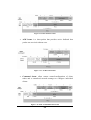
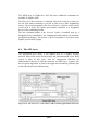
Figure 2.1 - NEC Electronics 16-bit Microcontrollers
with Embedded Radio Transceiver
Most of the microcontrollers today have native ability to interface with
sensors (built-in digital I/O and A/D converters). The 8-bit or 16-bit
microcontroller may already include 64 or even 256 kilobytes of flash
memory, RAM, and various hardware timers, along with the ability to
interface directly to the radio transceiver. The MCU requires few external
components to be fully functional.
Therefore, the silicon system size of a WSN node is usually smaller than the
batteries they use. This compact form factor lends itself well to innovative
uses of radio technology in sensor applications. Integration is the key issue,
and even higher levels of integration will be achieved in the future 802.15.4
platform.
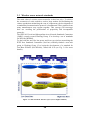
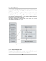
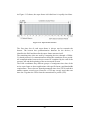
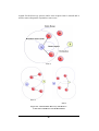
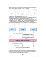
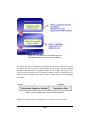
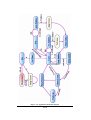
Figura 2.1 - A WSN taxonomy
30
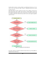
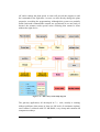
2.3 WSN application taxonomy
WSNs are mission-driven systems that provide a task efficiently. Since
WSN are service providers they can be modeled at different levels of
abstraction. To better understand the WSNs properties and characteristics
there is a need for a classification and definition of WSN applications.
To build such unambiguous classification scheme we start considering the
main properties of the systems.. This scheme is analogous to an objectoriented classification, where an object is described by its attributes and is
classified on the basis of its capabilities,. The properties of the wireless
applications are grouped into five categories: goal, interaction pattern,
mobility, space and time. Each of these are further classified to provide
sufficient details that are required for a typical WSN application.
The classification scheme is depicted in figure 2.1 while for a classification
of the WSN devices refers to[ChE06]
31
3
WSN classification and standards
3.1 A definition of WSN
A sensor network is an infrastructure include measuring, computing, and
communication elements that gives someone the ability to observe and react
to events in a specified environment. [SMZ07].
Thus a wireless sensor network (WSN) can be defined ([VDM06], [Cho06])
as a network of devices, possibly low-sized, denoted as nodes that can
measure some physical environmental phenomena and communicate the
information gathered from the monitored field through wireless links,
possibly via multiple hops relaying, to one or more sinks (named controller
or monitor) that can use it locally or is connected to other networks through
a gateway. The sink can be a common node or a specialized device with an
increased power computing and memory capabilities.
The nodes can be stationary or moving, aware of their location or not,
homogeneous or not.
Network sensor systems are seen as an important technology that will
experience major deployment in the next few years for a multitude of
applications discussed in the next paragraph.
There are four basic components in a sensor network [SMZ07]:
•
•
•
•
a set of distributed sensors;
an interconnecting network (in our case wireless-based);
a central point for coordination and of information processing;
a set of computing resources at the central point (or beyond) to
handle the data flow, correlation, event trending, status querying,
and knowledge discovery.
In this system the nodes, with sensing and computation capability, are
considered part of the sensor network as some of the computing may be
done in the network itself.
33
The algorithmic methods for data management, because of the large
quantity of data that can potentially be collected, play an important role in
WSN.
The computation and communication infrastructure associated with sensor
networks is often specific to this environment and rooted in the device and
application-based nature of these networks.
For example, unlike most other settings, in-network processing is desirable
in sensor networks; furthermore, node power (and/or battery life) is a key
design consideration.
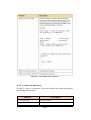
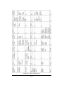
There are a number of different types of networks whose classifications
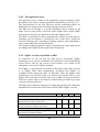
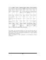
are based primarily on the distances they may reach [Lew04].You see in
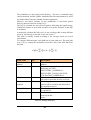
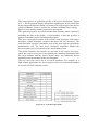
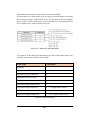
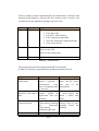
Table 3.1 how they relate to the wired world and to each other.
Table 3.1
Different Types of Networks
Network Type
Local Area
Network (LAN)
Wired
Wireless
IEEE 802.3 (Ethernet)
IEEE 802.11X
Personal Area
Network (PAN)
IEEE 1394 USB
Metropolitan Area
Network(MAN)
Broadband (DSL, cable)
IEEE 802.15.1
IEEE 802.15.3
IEEE 802.15.4
IEEE 802.16
Table 3.1 – type of network
The WSN discussed in this thesis are usually classified as WPAN
networks.
The IEEE (Institute of Electrical and Electronics Engineers) provides
standards for wired and wireless networking. The numbers are assigned by
the IEEE and become well known to industry users. The 802 series dictates
how each format must work. You can obtain lots of interesting information
about these standards and their use from various Web sites (like
www.dailywireless.org).
The IEEE formed the WPAN Study Group in 1998. The study group’s main
goal was to investigate the need for a wireless network standard for devices
within a personal operating space (POS). In the same year the Bluetooth
Special Interest Group (SIG) was formed. In 1999 the WPAN study group
became IEEE 802.15 (WPAN Working Group). The 802.15 WPAN
34
(Wireless Personal Area Network) is an effort to develop standards for short
distance wireless networks
These WPANs includes wireless networking of portable and mobile
computing devices, such as PCs, Personal Digital Assistants (PDAs),
peripherals, cell phones, and pagers, letting these devices communicate with
each other.
Since the formation of 802.15 four sub-projects have started, including
Bluetooth (Bluetooth 1.0 Specification in released in July of 1999) and the
co-existence of 802.11 and 802.15 networks, and 802.15.4 as well as a
standard for high bit rate (20 Mbps or higher) WPANs.
In general WSNs techniques (contention-oriented, channel sharing and
transmission) are now incorporated in the IEEE 802 family of standards,
indeed, these techniques were originally developed in the late 1960s and
1970s expressly for wireless environments and for large sets of dispersed
nodes with limited channel-management computing capabilities. [SMZ07]
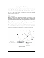
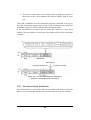
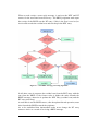
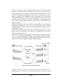
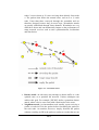
3.2 WSN classifications
A WSN as defined in paragraph 3.1 is a distributed systems (see [Cal06])
composed of several embedded devices, each equipped with a processing
unit, a wireless communication interface, and many sensors/actuators.
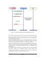
Figure 3.1 - single-sink WSN
35
Usually in these scenarios tiny battery powered devices are used, so that
deployment results easy and increase the global flexibility [Aky02],
providing low-cost, fine-grained interactions with the environment.
The result of the definition of WSN in paragraph 3.1 lead to a traditional
single-sink WSN (Figure 3.1).
Most of the scientific papers in the literature deal with such a definition but
this single-sink scenario suffers from an obvious bottleneck ([VDM06])
which implies a lack of scalability: increasing the number of nodes also the
amount of data gathered by the sink also increases and once its capacity is
reached the network size can not be augmented.
Furthermore, for reasons related to the MAC (medium access control) and
routing aspects discussed later, the global network performance cannot be
independent from the total network size.
3.2.1 Single-sink single-hop WSN
We can give an evaluation of the capacity of a single-sink single-hop WSN,
as in [VDM06], defined in terms of maximum number of nodes that a sink
can accept.
We consider a WSN where nodes are requested to send their samples
(composed of D bytes each) taken from the monitored space every TR
seconds. Initially we may assume that all nodes send their data directly to
the sink (a star topology). N Denote the number of nodes, Rb the channel bit
rate. Taking account of the overhead introduced by protocol stack layers, we
define a factor, αA≤ 1 thus if SA is the maximum data throughput measured
at the application layer, then will be SA= Rb·αA.
All protocol layers contribute to lower αA and reducing it will lower the
throughput even if the channel bit rate is unchanged. In modern
communication systems αA typically is a value between 0,5 and 0,1
[VDM06].
Under such assumptions, the application throughput will be approximately
equal to N·D·8/ TR . Thus, we arrive at the following inequality:
N·D·8/ TR ≤ Rb·αA
Therefore we can assert
(3.1)
N ≤ Rb·αA·TR /( 8D)
36
This equation rappresents an approximate estimation of the number of nodes
that can be part of a single-sink single-hop WSN. To give a numerical
example, assume R b = 250 Kbit/s,
TR = 1s, αA =0,1, D = 3; then the maximum number of nodes is
approximately 1000. On the other hand, if TR = 50 ms, then N can not
exceed 50.
As seen the requirements of the application play a relevant role when
defining the capacity of a single-sink WSN and also that the protocol
overhead can play a significant role, through αA.
In the case discussed above, the nodes are all within range of the sink. If the
transmission range of links between sink and nodes is R, then the density of
nodes for a bidimensional space is (no smaller than)
N / π R2 .
3.2.2 Single-sink multi-hop WSN
Now we will assume that the N nodes are distributed according to a smaller
density, thus some of them must reach the sink through multiple hops. If a
node can send its sample to the sink through h hops, then the delivery of the
data sample requires h transmissions.
Let us denote by hm the average number of hops per data sample taken from
the fi eld; if no smart reuse of radio resources is introduced, then we have
for a single-sink multi-hop WSN [VDM06]
(3.2)
N ≤ Rb·αA·TR /( 8Dhm)
Therefore, the capacity of the network is reduced by a factor of hm .
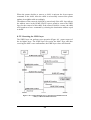
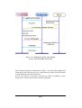
3.2.3 Multi-sink multi-hop WSN
A more general scenario includes multiple sinks in the network (see Figure
3.2 ). Maintaining the same node density, a larger number of sinks will
decrease the probability of isolated group of nodes that cannot deliver their
data due to an unfortunate signal propagation.
Moreover a multiple-sink WSN can be scalable: in fact, the same
performance can be achieved even by increasing the number of nodes, while
this is not true for a single-sink network.
Still a multi-sink WSN does not represent a trivial extension of a single-sink
case. There are mainly two cases:
37
All sinks are connected, wired or wireless, through a separate network,
The sinks are disconnected
Figure 3.2 -Multi Sink WSN
In the first case, a node needs to forward the data collected to any of the
sinks.
From the protocol viewpoint, this means that a selection can be done based
on a suitable criterion (e.g., minimum delay, maximum throughput,
minimum number of hops).
in this case the presence of multiple sinks ensures better performance then
the single-sink network with an equal the number of nodes in the same area,
but the communication protocols will be more complex.
In the second case, when the sinks are not connected, the presence of
multiple sinks just make a partition of the monitored field into smaller areas;
however from the communication protocols viewpoint there are no
significant changes, apart from simple sink discovery mechanisms.
Because of the better potential performance, the first case is clearly the most
interesting due to the sinks connected through any type of mesh network is
clearly the most interesting case.
We can do an approximate evaluation of the capacity of a multi-sink WSN,
assuming that each sink (denoting as NS their number in the network) can
serve N nodes with N limited by expressions (3.1) and (3.2).
We can assert:
38
(3.3)
N ≤ NsRb·αA·TR /( 8Dhm)
assuming that group of nodes attached to a given sink do not interfere with
those attached to other sinks. To give a numerical example we will use the
same value as for the single sink case: Rb = 250 Kbit/s, T R = 50 ms, αA =
0,1, D = 3; then, if there are NS = 5 sinks in the network, the maximum
number of nodes is about 250.
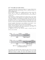
3.2.4 Actuators
Both the single-sink and multiple-sink networks reviewed above do not
include the presence of actuators, namely devices able to manipulate the
environment rather than observe and measeure it. WSANs are composed of
both sensing and actuators nodes (see Figure 3.3 ).
The inclusion of actuators doesn’t represent a simple extension of a WSN.
In fact from the communication protocol point of view the data-flow must
go to the opposite direction in this case:
when sensors provide data the protocols should be able to manage many-toone communications, and one-to-many when the actuators need to be
controlled. The complexity of the protocols in this case is even greater.
Figure 3.3 - WSAN
39
3.3 Wireless sensor network standards
The main value of wireless sensor networks is their low price. To achieve
the economies of scale needed to reach a large market and facilitating the
volume production minimizing the cost of components, the development of
a standardized communication protocol is fundamental. Thus products from
many manufacturers may operate together. This synergy will encourage
their use avoiding the proliferation of proprietary and incompatible
protocols..
The IEEE 802 Local and Metropolitan Area Network Standards Committee
(LMSC) recently created Working Group 15 to develop a set of standards
for WPANs [BGH00].
To deal with the need for low-power and low-cost wireless networking the
IEEE New Standards Committee (NesCom) officially funded a new task
group in Working Group 15 to begin the development of a standard for
Low-Rate WPANs (LR-WPANs), called 802.15.4 (see Fig. 3.4 for more
details).
Figure 3.4 - 802 Standards' Wireless Space (source ZigBee Alliance)
40
The goal of this group was to provide a standard having ultra-low
complexity, cost, and power for low-data-rate wireless connectivity among
inexpensive, fixed, portable, and moving devices [IEE03].
The main target of Task Group 4, as for all IEEE 802 wireless standards,
was limited to the creation of specifications of the Physical (PHY) layer and
Media Access Control (MAC) sub-layer of the Data Link Layer in the
International Standards Organization (ISO) Open Systems Interconnection
(OSI) reference model. In May 2003 the 802.15.4 standard was approved.
3.3.1 The IEEE 802.15.4 low-rate wpan standard
As noted in the previous paragraph, the scope of the IEEE 802.15.4 task
group, as defined in its original Project Authorization Request, is to “define
the PHY and MAC specifications for low data rate wireless connectivity
with fixed, portable and moving devices with no battery or very limited
battery consumption requirements typically operating in the Personal
Operating Space (POS) of 10 meters.”
Moreover the purpose of the project is “to provide a standard for ultra low
complexity, ultra low cost, ultra low power consumption and low data rate
wireless connectivity among inexpensive devices. The raw data rate will be
high enough (maximum of 200 kbps) to satisfy a set of simple needs such as
interactive toys, but scaleable down to the needs of sensor and automation
needs (10 kbps or below) for wireless communications.” [Mid00]
The maximum and minimum raw data rates were later raised respectively to
250 and 20 kb/s.
This diverse set of goals requires the IEEE 802.15.4 standard to be
extremely flexible.
The IEEE 802.15.4 standard supports a large variety of possible applications
in the POS Unlike protocols such as IEEE 802.11 that are designed for a
single application.
The possible applications vary from those requiring high data throughput
and low latency to those requiring very low throughput and able to tolerate
significant message latency.
The IEEE 802.15.4 standard supports peer-to-peer and star connections, and
is able to support a wide variety of network topologies. When security it is
required that is entrusted to the AES-128 algorithm (see [Nis01] for more
information about AES).
The standard includes optionally beacons (see Appendix A), with a variable
beacon period that is a binary multiple of 15.36 ms, up to a maximum of
15.36 ms × 214 = 4 minutes and 11.65824 seconds, thus that the optimum
trade-off can be made between message latency and network node power
consumption. When applications have duty cycle (see Appendix F)
41
limitations the beacons can be omitted as, for example, may happen on
networks in the 868 MHz band, which has law limits on node duty cycle, or
systems that require nodes with constant listening mode.
The channel has a contention based access, the mechanism use a carrier
sense multiple access with collision avoidance (CSMA-CA), if beacon is
used it will be followed by a contention access period (CAP) for devices
attempting to gain access to the channel, the length of the CAP is a fraction
of the period between beacons.
The CAP may be limited to a fixed time of approximately 2 ms by a
“battery life extension” mode.
When an application requires low message latency, the standard employs
the optional guaranteed time slots (GTSs), which reserve channel time for
devices without follow the CSMA-CA access mechanism.
A 16-bit address field is used to address the devices, meaning that up to (28 2) × (28 - 2) = 64,516 logical addresses (two values in each byte are
reserved);
Therefore the standard also includes the ability to send messages with 64-bit
extended addresses, allowing a sufficient number of devices for any
application to be placed in a single network.
The messages can be fully acknowledged and in this case each transmitted
frame (excepted the beacons and the acknowledgments themselves) may
receive an explicit acknowledgment.
The overhead introduced with explicit acknowledgments is usually
acceptable given the low data throughput typical of wireless sensor
networks and the results is a reliable protocol.
Moreover the acknowledgments may optionally support the passive
acknowledgment techniques, used in some ad hoc routing schemes, for
example, the gradient routing (GRAd) algorithm (discussed later in this
chapter).
Several features is designed to minimize power consumption are
incorporates in the IEEE 802.15.4 standard.
Besides the use of long beacon periods and the battery life extension mode,
the active period of a beaconing node can be drastically reduced (according
to a powers of two), allowing the node to sleep within two beacons.
One important goal in the design of the IEEE 802.15.4 was the coexistence
with other device and services using the same unlicensed bands.
As evidence the dynamic channel selection is implemented in the protocol,
so if an interference from other services appear on a channel used by an
IEEE 802.15.4 network, the network coordinator ( PAN coordinator) scans
the other available channels to find a the suitable channel.
In this scan, The coordinator obtains a measure of the peak energy present
in each channel and then uses this information to select a free channel.
42
This channel selection scan can also be used prior to the establishment of
the network or even prior to each frame transmission (except beacon or
acknowledgment frames). Each network node must complete two clear
channel assessments (CCAs) as part of the CSMA-CA mechanism to ensure
the channel is unoccupied prior to transmission.
A link quality indication (LQI) byte is appended to each received frame by
the PHI layer before it is sent to the MAC layer. This information may be
used by receiving nodes for several purposes, at the discretion of the
network designer and according to application needs.
Figure 3.5- Network topologies and node types
For example, the LQI can be used as an indication of channel noise, perhaps
leading to a dynamic channel selection process and move to another free
channel or it can be used for power control of its own transmitter (assuming
a symmetrical channel). It may be also used as part of a network routing
algorithm based on link quality between network nodes or to estimate the
location of each network node relative to its peers.
The LQI may be generated indifferently from a signal level determination, a
signal-to-noise determination, or a combination of the two. This enables
received signal strength indication (RSSI) and signal quality estimators to
be used together.
Although a byte is reserved for the LQI, to ease the burden on developers
that do not desire to make use of it (appropriate for some applications), the
IEEE standard specifies that at least eight unique values shall be used in the
LQI, including 0 × 00 and 0 × FF are to be associated respectively with the
lowest and highest quality 802.15.4 signals detectable by the receiver.
43
To maximize the utility of the IEEE 802.15.4 tried to balance the desire to
enable small, low-cost, and low-power network nodes with the needs to
produce a standard that met a wide variety of on-field applications.
The resulting standard includes three types of network node functionality:
•
PAN coordinator. The PAN coordinator is the node that initiates
the network and is the controller of the network. The PAN
coordinator may transmit beacons and can communicate with all the
device in range. Depending on the network design, it may have
memory sufficient to store information on all devices in the network,
and must have memory sufficient to store routing information as
required by the algorithm employed by the network.
•
Coordinator. The coordinator may transmit beacons as the PAN
coordinator and can communicate directly with any device in range.
A coordinator may become or be promoted to PAN coordinator and
start a new network.
Device. A network device does not beacon and can directly
communicate only with a coordinator or PAN coordinator.
•
These three functions are to be encapsulated into two different device types:
•
Full function device (FFD)). An FFD can operate in any of the three
network roles (PAN coordinator, coordinator, or device). It must
have sufficient memory to store routing information as required by
the algorithm employed by the network.
•
Reduced function device (RFD). An RFD is a very low cost device,
with minimal memory requirements. It can only function as a
network device.
Wireless light switch is a typical example of a RFD. It must be as
inexpensive to produce as possible, and has limited functional requirements.
The light itself, however, may be the archetypical FFD because it can be
more expensive, has access to mains power, and can have additional
network functions as a more permanent feature of the building [Cal06].
The IEEE 802.15.4 standard, as said before, supports multiple network
topologies.
In the standard, two network types are discussed: star networks and peer-topeer networks. In the star network, the master device is the PAN coordinator
(FFD node), and the other network nodes may either FFDs or RFDs.
44
In the peer-to-peer network, FFDs are usually used, one of them is the PAN
coordinator. RFDs may be used in a peer-to-peer network, but they can only
communicate with a single FFD belonging to the network, and so do not
have a real “peer-to-peer” communication.
Similar to all IEEE 802 wireless standards, the IEEE 802.15.4 standard
standardizes only the physical and medium access control (MAC) layers.
In fact the IEEE 802.15.4 standard incorporates two physical layers:
•
The lower band: the 902–928MHz, for most of the Americas and
pacific lands, 868.0–868.6 MHz (for Europe),
•
The upper band: 2.400–2.485 GHz (worldwide with marginal
differences in the band boundary)
The channel numbers and their center frequencies are defined as follows:
Figure 3.6- 802.15.4 channels (from ZigBee Alliance)
FC = 868.3 Mhz, for k = 0
FC = 906 + 2 (k-1) Mhz, for k = 1,2,…,10
FC = 2405 + 5 (k-11) Mhz, for k = 11,12,…,26
45
3.4 Protocol layers
As noted before, the IEEE 802.15.4 standard incorporate two distinct layers,
the physical (usually simply called PHY) and the medium access control
(MAC) layer.
However, to easily build an application without the need of a low level
knowledge about the node structure, at least two more layers are required:
the Data-link layer and Network layer. Thus a Alliance between some of the
major industry was born to promote a 802.15.4 based standard containing
the two more layers (see fig. 3.6 and 3.10).
The ZigBee standard will be discussed later in this chapter, now we will
focus on the two IEEE 802.15.4 layers.
Figure 3.7 - OSI Data link layer architecture
3.4.1 The physical (PHY) layer
The physical layer (PHY) of the reference model specifies the network
interface components, their parameters, and their operation.
46
Moreover, to support operation of the MAC layer, the PHY layer includes a
variety of features, such as receiver energy detection (RED), link quality
indicator (LQI), and clear channel assessment (CCA).
Parameter
2.4-GHz PHY
868/915-MHz PHY
Sensitivity @ 1%
PER
Receiver
maximum input
level
Adjacent channel
rejection
Alternate channel
rejection
Output power,
lowest maximum
Transmission
modulation
accuracy
Number of
channels
Channel spacing
-85 dBm
-92 dBm
Transmission rates
Symbol rate
Bit per symbol
Symbol period
Chip rate
Chip modulation
Chip pseudo-noise
sequence
RX-TX and TXRX turnaround
time
-20 dBm
0 dB
30 dB
-3 dBm
EMV < 35% for
1000 chips
16
1/10
5 MHz
NA(Single
channel)/2 MHz
20/40 kbps
20/40
kilosymbols/sec
1
49 µs/24 µs
300/60 kilochips/sec
BPSK with raised
cosine pulse shaping
Date rate 250 kbps
62.5
kilosymbols/sec
4
16 µs
2 megachips/sec
O-QPSK with halfsine pulse shaping
(MKS)
32
15
12 symbols
Table 3.2 IEEE 80215.4 PHY Layer Main Parameters
47
The PHY layer is provided by a wide range of operational low-power
features, including low-duty-cycle operations, strict power management,
and low transmission overhead [SMZ07]. These parameters are listed in
Table 3.2.
The two PHY bands, viewed in the paragraph 3.3.1, employ a form of direct
sequence spread spectrum (DSSS).
The DSSS is one of the spread spectrum modulation techniques, and as all
these kind of techniques, use a carrier signal that occur on the full device’s
transmitting bandwidth (the so called spectrum) thus the modulation occupy
more bandwidth than the information signal itself.
DSSS provides a higher data rates and shorter delays than FHSS (the
frequency hopping technique also used in wireless transmission see
appendix A for more information about FHSS), because the device don't
spend time retuning.
The spread-spectrum techniques are resistant to interference, signals that
stay in one narrow area (and don’t move), but they don’t do as well when
other spread spectrum systems are operating nearby.
Figure 3.8- DSSS modulation technique
In our case DSSS is resistant to interference via the spreading function that
concentrate the desired signal but spread and dilutes any interfering signal,
however few nearby FHSS systems are sufficient to cripple a DSSS system,
on the other hand, because a DSSS system is transmitting on every
frequency in the band, a nearby FHSS system will be unable to find any
clear channel to use.
FHSS usually degrades more gracefully than DSSS in the presence of
interference but neither works well when competing at close range.
48
DSSS transmission is generated multiplying the data by a noise signal
generated as a pseudorandom sequence of 1 and -1 values. This noise signal
has a much higher frequency than the information signal.
Direct-sequence spread-spectrum transmissions multiply the data being
transmitted by a noise signal.
The noise-like signal can be used by receiver to reconstruct the original
data, by multiplying it by the same pseudorandom sequence (because 1 × 1
= 1, and −1 × −1 = 1). This process is known as de-spreading.
To work correctly, the transmit and receive sequences must be synchronized
via some sort of timing process.
Application
Frequency Band Used
AM radio
Analog cordless telephone
Television
FM radio
Television
Television
Wireless data
Cellular
Digital cordless
Personal communications
Nationwide paging
Satellite telephone uplink
Personal communications
Satellite telephone downlink
IEEE 802.11b/g wireless LANs
IEEE 802.15.4/Zigbee alliance
IEEE 802.16/WiMax
IEEE 802.11a wireless LANs
Large dish satellite TV
Small dish satellite TV
Wireless cable TV
535–1635 kHz
44–49 MHz
54–58 MHz
88–108 MHz
174–216 MHz
470–806 MHz
700–720 MHz
806–890 MHz
900 MHz
900–928 MHz
929–932 MHz
1610–1625.5 MHz
1850–1990 MHz
2.4835–2.5 GHz
2.4 GHz
2.4 GHz
2–66 GHz
5 GHz
4–6 GHz
11.7–12.7 GHz
28–29 GHz
Table 3. 3 - Common Wireless Applications and Their Frequencies
If a second transmitter use the same channel but with a different noise
sequence, the de-spreading process results in no processing gain for that
signal, allowing multiple DSSS transmitters to share the same channel
within the limits of the cross-correlation properties of their sequences. In
table 3.3 can be seen the frequency commonly used by wireless
applications.
49
3.4.2 Packet structure
The packet structure of the IEEE 802.15.4 PHY layer is shown in fig.
3.9. The first field of this structure contains a 32-bit preamble used for
symbol synchronization. The next field contain a 8-bit value used for frame
synchronization and represent a start of a packet delimiter. The PHY header
(8-bits) field specifies the length of the PHY service data unit (PSDU) that
can carry up to 127 bytes of data.
Figure 3.9- 802.15.4 PHY-layer packet structure
The total packet transmission time is about 4,3 ms at 250kbps or 52 ms at
40kbps (the two typical bands).
3.5 The medium access control (MAC) layer
As already mentioned the need to conserve energy is the most critical issue
in the design of MAC layer protocol for WSNs.
Several factors may contribute to energy waste such as idle listening, packet
collisions, and overhearing.
The media access regulation requires the exchange of control and
synchronization information between the competing nodes. The exchange of
a large number of control and synchronization packets may result in a
significantly increase of energy consumption. On the other hand long
periods of idle listening may decrease network throughput increasing energy
consumption.
In some cases the energy wasted by idle listening is equal to one-half of the
total energy consumed by a sensor during its lifetime. [Bou08]
Another source of significant energy waste is the retransmission of colliding
packets. Moreover a high number of collisions may lead to significant
performance degradation.
50
The excessive overhearing yet causes a node to receive and decode packets
intended for other nodes increases energy consumption and degrading the
network throughput.
The main objective of a WSN MAC-layer protocols is to reduce such
energy waste discussed above.
These protocols can be categorized into two main groups:
•
schedule-based MAC-layer protocols: these protocols are a class of
deterministic protocols in which the channel access is based on a
schedule. Channel access is limited to one sensor node at a time.
This is achieved by a resources pre-allocation to individual nodes.
•
contention-based MAC-layer protocols: these protocols avoid preallocation of resources. Instead, a single radiochannel is shared by
all nodes and allocated on demand. However each simultaneous
attempts to access the communications channel results in collision.
The main objective of contention-based MAC layer protocols is to
minimize the occurrence of collisions, rather than completely avoid
them.
To reduce energy consumption, these protocols differ in the mechanisms
used to reduce the possibility of a collision while minimizing overhearing
and control traffic overhead.
Resolving collisions is usually achieved using distributed, randomized
algorithms to reschedule channel access among competing sensor nodes.
The basic approach used to reduce overhearing is to force nodes into a sleep
state when they become inactive. [SMZ07]
Communication between wireless sensor nodes is usually achieved by a
unique channel. Usually only a single node can transmit a message at any
given time using this channel, so the shared access of the channel requires a
protocol among the nodes. The MAC protocol is designed to regulate access
to the shared wireless medium such that the performance requirements of
the application are satisfied.
From the perspective of OSI Reference Model, the MAC functionalities are
provided by the lower sublayer of the data link layer (DLL).
The higher sublayer of the DLL is referred as the logical link control layer
(LLC). The presence of the LLC sublayer allows support for several MAC
options, depending on different characteristics as network topology used,
type of communication channel, quality of service requirements.
The MAC sub layer resides directly above the physical layer (see fig. 3.6
and 3.10) and perform the following three functions [SMZ07]:
51
•
•
•
Assembly of data into a transmitting frame by appending a header
field containing addressing information and a trailer field for error
detection
Disassembly of a received frame to extract addressing and error
control information to perform address recognition and error
detection and recovery
The regulation of access to the shared transmission medium
Figure 3.10- Stack Reference Model and their relative tasks
The LLC sub layer of the DDL provides a direct interface to the upper layer
protocols. Its main objective is to shield the upper layer protocols from the
characteristics of the underlying physical network. The use of the LLC
sublayer is very limited as interoperability is usually achieved by other
network layer protocols.
The IEEE 802.15.4 MAC-layer specification is designed to support a
large variety of industrial and home applications for control and monitoring
as previously discussed (see paragraph 2.2). These applications usually
require low to medium data rates and moderate average delay and high
flexibility. moreover, the complexity and implementation cost of the IEEE
802.15.4 standard compliant devices must be low to minimize energy
consumption and enable large scale production of these devices.
To achieve these goals IEEE 802.15.4 MAC-layer specification embeds in
its design several features for flexible network configurations and lowpower operations.
52
These features include [SMZ07]:
•
•
•
•
•
•
•
Various network topologies and devices support
Optional super-frame structure to control the network devices’ duty
cycle
Direct and indirect data transmissions
Contention- based and schedule-based MAC methods
Beaconed and non-beaconed modes of operation (beacon mode uses
a super-frame structure to coordinate access to the medium. Support
for contention-based access and guaranteed time slots allocation; in
non-beaconed mode, the protocol uses an unslotted CSMA/CA
based access scheme.)
Efficient energy management schemes for an extended battery life
that includes adaptive sleep for period of time over multiple beacons
Flexible addressing scheme to support the deployment of large-scale
networks (over 65,000 nodes per network)
Based on the logical devices types seen in paragraph 2.4.1, a IEEE 802.15.4
wireless personal area network can be organized in one of three possible
topologies: star, mesh (peer-to-peer), or cluster tree. The three network
configurations are depicted in figure 3.5. The star network topology
supports a single coordinator, with up to 65,536 devices.
In this topology configuration, one of the FFD-type devices assumes the
role of network coordinator. All other devices act as end devices.
The selected coordinator is responsible for initiating and maintaining all the
end devices on the network.
The end devices can only communicate with the coordinator. The mesh
configuration allows path formation from any source device to any
destination device, using tree and table-driven routing algorithms.
distance vector routing (AODV) and Internet Engineering Task Force
(IETF).
In the mesh topology the radio receivers of the PAN coordinator and the
routers must be always active.
Cluster tree networks enable a peer-to-peer network to be formed using
multihop routing.
A cluster tree network is self-organized and supports network redundancy to
achieve a high degree of fault tolerance and self-repair. The cluster tree
topology fits latency-tolerant applications.
The cluster can be significantly large, comprising up to 255 clusters of up to
254 nodes each ( for a total of 64.770 nodes).
The routing algorithm employs a simplified version of the on-demand
53
Any FFD can be a coordinator. The PAN coordinator, chosen from one of
the coordinators, build up the first cluster and assigns to it a cluster identity
(CID) of value zero. All other clusters are then formed with a designated
cluster coordinator for each cluster.
Each PAN is uniquely identified by a 16-bit identifier. A PAN coordinator
is designated as the controller of the WPAN.
Every network has exactly one PAN coordinator, selected from within all
the coordinators of the network.
A coordinator is a device configured to support advanced network
functionalities including:
•
Managing a list of all associated network devices
•
Exchanging data frames with network devices and a peer coordinator
•
Allocating 16-bit short addresses to network devices
•
Generating beacon frames on a periodic basis (used to announce the
PAN identifier, and other network and device parameters.)
Must be noted the MAC layer offers channel scan capability and not only
and association/disassociation functionalities. This scan procedure work on
several logical channels by sending a beacon request message and listening
or just listening in case of a passive scan (RFD nodes) for beacons to locate
other PANs coordinators.
The higher protocol’s layers decide which PAN to join and ask the MAC
layer to provide the association procedure for the selected PAN/channel.
The MAC layer send a join request to one of the network coordinators and if
accepted the node receives his address that it may use for all communication
purposes.
3.5.1 Frame and super-frame structure
The MAC layer provides four frame form structures, one for each type of
message that can be sent:
•
Data frame: provides up to 104 byte data payload capacity, include
a sequence numbering to ensure that packets are tracked and a Frame
Check Sequence (FCS) validates error-free data.
54
Figure 3.11- Data Frame Format
•
ACK frame: is a short packet that provides active feedback that
packet was received without error
Figure 3.12 - ACK Frame format
•
Command frame: allow remote control/configuration of client
nodes and a centralized network manager to configure individual
clients.
Figure 3.13- MAC Command frame format
55
Command Frame
Identifier
00000001
00000002
00000003
00000004
00000005
00000006
00000007
00000008
00000009
Command
Association request
Association response
Disassociation notification
Data request
PAN ID conflict notification
Orphan notification
Beacon request
Coordinator realignment
GTS request
RFD
TX RX
X
X
X
X
X
X
X
X
Table 2.4 - MAC Commands
•
Beacon data frame: client devices can wake up only when a beacon
is to be broadcast, listen for their address, and if not heard, return to
sleep. Beacons are important for mesh and cluster tree networks to
keep all of the nodes synchronized without requiring nodes to
listening for long periods of time and consume battery energy.
The frames are depicted in the fig 3.11-3.14
As already mentioned the IEEE 802.15.4 MAC defines an optional superframe structure. When used it is initiated by the PAN coordinator.
Furthermore, its format is decided by the coordinator.
Figure 3.14 - Beacon data frame format
56
As Figure 3.15 shows, the super-frame is divided into 16 equally sized slots.
Figure 3.15 - Super-frame structure
The first time slot of each super-frame is always used to transmit the
beacon. The beacon has synchronization function for the devices, it
identifies the PAN and describe the super-frame structure itself.
The remaining time slots are used by competing devices, through a CSMACA based protocol, for communications during the contention access period.
All communications between devices must be completed by the end of the
current CAP and the beginning of the next network beacon.
The PAN coordinator may dedicate groups of contiguous time slots of the
active super-frame to these applications with specific latency and bandwidth
requirements. These slots are named guaranteed time slots (GTSs) and their
number cannot exceed seven. However a GTS may occupy more then one
time slot. Together the GTSs form the contention free period (CFP).
57
Figure 3.16 - Super-frame with GTSs
The CFP always appears at the end, of the active super-frame and starts at a
slot boundary immediately following the CAP, as depicted in Figure 3.16.
The CAP time slots still remain for contention-based access between
devices and new devices trying to join the network.
All communication transactions using contention-based access and GTSbased access must respectively complete before the end their associated
CAP and CFP.
Network devices can send requests for GTS allocation during the CAP
period to reserve contiguous time slots, either the receive (from the
coordinator) or transmit (to the coordinator) data.
Devices can switch off their power and go into a sleep mode when have no
data to send. However devices are must to remain active, during their
allocated GTSs but are allowed to go into a sleep mode during the other
GTSs periods.
The coordinator may also send a super-frame containing both an active and
an idle period to reduce energy consumption, as shown in figure 3.17.
The active period, always composed by the 16 time slots, contains the frame
beacon, the CAP time slots and the CAP slots when applicable. The inactive
period defines a configurable time period during which all network nodes,
including the coordinator, can go into a sleep mode switching off their
power and set a wake up timer to the next beacon frame (just before it).
Summarizing the general MAC frame format is composed of three basic
components: a header, a payload, and the footer.
58
Figure 3.17 - Super-frame with inactive period
The MAC header contains a frame control field and the address field. The
control field carries the frame type and other information necessary for
network control and operation. The address specifies the source PAN
identifier and source node address, the destination PAN identifier and
address.
The MAC payload contains the data frame to be exchanged between the
communicating devices. The MAC footer contains the frame check
sequence field and is also used to detect frame errors.
3.5.2 The association request and response command formats
The association command is part of the MAC association services and is
formed by association request and response illustrated in Figure 3.18.
The capability information field of the association request supply
information about many questions regarding the device that requested to
join the network:
•
•
•
•
The device is a PAN coordinator, the alternate PAN coordinator
field is set to zero if the device cannot act as a PAN coordinator.
Is this node an FFD or an RFD device, if the device type field is set
to one, the device is an FFD.
The device is battery powered or connected to a main power source,
for battery powered nodes, the power source field is set to zero.
The device keep its receiver in ON mode all the time or turn off the
receiver and go to power-saving mode when the device is idle. The
receiver is ON when idle field is set to zero if the receiver is turned
off during idle mode. The value of this field comes from the MAC
attribute macRxOnWhenIdle and is equal to FALSE if the receiver is
turned off during idle mode.
59
•
The device want to have a new address after joining the network. If
the device needs a short address, the allocate address field is set to
one.
The PAN coordinator uses the association response command to accept or
deny the association request from a node. If the coordinator has reached its
maximum capacity it will be indicate in PAN capacity status.
If the association is accepted and the node also asked for a new short
address, the short address is sent in the short address field of the association
response.
Figure 3.18 - The Association Request Command (a)
and The Association Response Command (b)
3.5.3 The Disassociation Notification
The disassociation is a procedure that an associated node uses to notify the
parent or the coordinator that the device itself wants to leave the network .
60
Figure 3.19 - MAC Disassociation Notification Command
The disassociation frame format is depicted in Figure 3.19. A device will
leave a network based on either its own decision or the request of the
parent/coordinator (for instance when the parent itself wants to leave the
network).
3.5.4 Security
The security services specified by the IEEE 802.15.4 model provide support
for infrastructure security and application data security. There are four kind
of services:
• The first security service of provides support by preventing
unauthorized parties from joining the network and allows a device to
maintain a list of network trusted devices. This list is used by any
network node to detect and reject messages from unauthorized
devices.
• The second security service supports message integrity protection to
prevent the tampering attempt of a legitimate data message from an
authorized sender while the message is in transit (by any kind of
intruder).
• The third security service provides the data confidentiality of e
message. This is achieved implementing the a 128-bit key advanced
encryption standard (AES) cryptographic algorithm.
• The fourth security service deals with sequential data freshness to
prevent replay attacks, where an unauthorized party resend
legitimate messages at a later time.
The MAC layer describes a variety of security suites, based on this four
security services, each one offering a different set of security properties and
guarantees. The MAC standard specify that the security is not enabled by
default and the application must explicitly set the appropriate parameters to
enable the desired security level.
61
3.6 ZigBee standard
ZigBee and IEEE 802.15.4 are standards-based protocols that provide the
network infrastructure required for wireless sensor network applications.
ZigBee is a trademark like Wi-Fi and WiMAX and its stack, shown in
figure 3.20, only defines some functionalities in layers on top of the IEEE
802.15.4 standard.
The IEEE 802.15.4 standard has been adopted by the ‘ZigBee Alliance’ for
wireless personal area network technology. “The Alliance is an association
of hundreds of members from around the world, working together to enable
the reliable and cost-effective networking of wireless devices for monitoring
and control, based on an open global standard” [Kin05].
802.15.4 defines the physical and MAC layers, and ZigBee defines the
network and application layers. Using the IEEE 802.15.4 specifications,
allow the alliance to focus on the design issues.
3.6.1 The network layer (NWK APL)
ZigBee Alliance provides the network layer (NWK) and some applications,
and differentiates between a usual node, a coordinator and a router. The
only difference between the last two is based on the connection to some
external network.
The NWK and addresses three main items via ZigBee Device Objects
(ZDOs):
The role of discovery is, as the name suggests, to discover nodes and then
they use unicast messages to inquire about the ZigBee coordinator’s or
router address. This may also query about addresses of other associated
devices. There is also a broadcast inquiry for the coordinator’s/router
addresses.
Must be noted that there is a distinction between the MAC and the network
addresses, clearly IP but the field is left open for any proposal.
62
Figure 3.20- ZigBee stack architecture
•
Service discovery
•
Security
•
Binding
The equivalent of the Address Resolution Protocol (ARP) is also supported
in ZigBee by a similar mechanism: a broadcast with the network or the
MAC address shall return the other missing one.
ZigBee use profiles like Bluetooth but is more evolved. A profile defines the
applications running on top of a device where it also specifies the members
and the possible actions. So it is a set of device requirements, collaborating
to fulfill a role. An example could be a thermometer, a blood pressure
probe, and a console together forming a patient monitoring application
[LAD07].
63
Figure 3.21- ZigBee extended architecture
As profiles play an important roles in ZigBee, the discovery on the other
hand allow the locating procedure for some services via their profile
identifiers.
The security services in ZDO have the role to authenticate and derive the
necessary keys for data encryption. Thus ZigBee complements IEEE
802.15-4 for security.
The encryption key is used as in Bluetooth to authenticate and derive a
shared secret, named ‘link key’. An initiator device and a responder have a
pre-established trust. Three more steps follow this trust establishment: an
exchange of test data, derivation of the link key and a confirmation.
The master secret shared between devices could be sent before with an outof-band channel. It’s called a proximity authentication channel and is used
in several similar protocols.
Another ZDO’s component is the network manager, implemented in the
coordinator and it allow the selection of an existing PAN to interconnect.
Furthermore it provides the creation of new PANs and implements also a
routing algorithm between routers of different PANs that it has discovered.
The binding manager is last component and has the role to bind nodes to
resources and applications and to bind devices to channels in order to
calculate the remaining available bandwidth a coordinator can grant on the
link.
64
3.6.2 The application layer
The application layer consists of the application support sub-layer (APS),
the ZigBee device object, and the application-defined objects (see fig 3.21).
The responsibilities of the APS sub-layer include maintaining tables for
binding devices together and forwarding messages between devices.
The ZDO can be thought as a special application object resident on all
nodes. It has its own profile, referred to as the ZigBee device profile (ZDP)
that can be accessed by user application and other ZigBee nodes.
The ZDO is responsible for device management, security keys and policies,
including, but not limited to, defining the role of the device within the
network, initiating and responding to binding requests, and establishing a
secure relationship between network nodes.
The designer-defined application objects implement the actual applications
according to the ZigBee-defined application descriptions.
3.6.3 ZigBee Versions from 2004 to PRO
In conclusion we can say that the main goal in developing ZigBee
technology was to provide a standard for the operation of remote monitoring
sensor devices and for this reason several features were added in the
subsequent version of the ZigBee standard
The ZigBee 1.0 specification was ratified in December 2004, and is referred
to as ZigBee 2004. Most manufacturer developed their ZigBee 1.0
compliant library during the 2005. In December 2006, the ZigBee 2006
specification was released, which was followed in October 2007 by the
ZigBee 2007 and at the end of the same year by PRO version specification.
Each new release adds to and improves functionality provided in previous
versions of the specification.
The table below illustrates a high-level comparison showing the similarities
and differences between the 2004, 2006, and 2007/PRO ZigBee versions.
2004
Interference avoidance
Coordinator selects best available RF Yes
channel/Network ID at startup time.
RF channel and/or Network ID can be changed
during operation to address interference.
Automated/distributed address management
Addresses automatically assigned using Yes
hierarchical, distributed scheme.
65
2006
2007
PRO
Yes
Yes
Yes
Yes
Yes
Yes
Yes
Addresses automatically assigned using
stochastic scheme
Group addressing
Devices can be assigned to groups, which can be
addressed with a single frame; thereby reducing
network traffic for packets destined for groups.
Centralized data collection
Low-overhead data collection by ZigBee
coordinator supported
Low-overhead data collection by other devices
supported under special circumstances (e.g. with
Tree Routing).
Many-to-one routing allows the whole network
to discover the aggregator in one pass.
Source routing allows the aggregator to respond
to all senders in an economical manner
Security
128-bit AES encryption with 32-bit Message
Integrity Code (MIC)
Frame counters to assure message freshness
Security applied at the NWK layer by default,
and supported at higher layers.
Key rotation prevents hacking of NWK key.
Trust Center operates on the ZigBee Coordinator
to manage trust on behalf of network devices
and act as central authority on which devices can
join the network.
High Security mode supported, which is
selectable by Trust Center policy, and requires
Application Layer Link Keys, peer-entity
authentication, and peer-to-peer establishment
using Master Keys.
Trust Center can run on Coordinator or any
other device in the network.
Network scalability
Addressing algorithm supports networks with
tens to hundreds of devices.
Addressing algorithm supports networks with
hundreds to thousands of devices.
Message size
< 100 bytes, with exact size depending on
services employed (e.g. security).
Large messages, up to the buffer capacity of the
sending and receiving devices (supported using
Fragmentation and Reassembly
66
Yes
Yes
Yes
Yes
Yes
Yes
Yes
Yes
Yes
Yes
Yes
Yes
Yes
Yes
Yes*
Yes
Yes
Yes
Yes
Yes
Yes
Yes
Yes
Yes
Yes
Yes
Yes
Yes
Yes
Yes
Yes
Yes
Yes
Yes
Yes
Yes
Yes
Yes
Yes
Standardized commissionino
Standardized start up procedure and attributes
support the use of commissioning tools in a
multi-vendor environment.
Robust mesh networking
Fault tolerant routing algorithms respond to Yes
changes in the network and in the RF
environment.
Every
device
keeps
track
of
its
“neighbourhood”; thereby improving reliability
and robustness.
Cluster Library support
The ZigBee Cluster Library, as an adjunct to the
stack, standardizes application behaviour across
profiles and provides an invaluable resource for
profile developers.
Yes
Yes
Yes
Yes
Yes
Yes
Yes
Yes
Yes
Yes
* AES in version 2004 is optional and not activate by default
Table 3. 5- ZigBee changes from 2004 to PRO version (source [Dai08])
About the backward compatibility
the first ZigBee 1.0 original
specifications were abandoned and the compatibility is not assured as we
can see from the below list, while is required a backward compatibility from
the 2007/PRO versions toward the 2006 specifications:
ZigBee 2007/PRO:
• Backward compatibility with ZigBee 2006 required.
• Backward compatibility with ZigBee 2004 not required.
ZigBee 2006
• Backward compatibility with ZigBee 2004 not required.
ZigBee 2004
• Original ZigBee version.
3.6.4 Brief comparison with other protocols
As previously noted ZigBee focuses on large scale monitoring applications
in which nodes require a low data rate and very low power consumption.
ZigBee protocol can be used to connect the ZigBee nodes to be integrated
with the IP networks. This approach enables remote sensing and controlling
on the Internet.
67
Technologies such as the well known Wi-Fi target devices running
applications that require large amounts of data to be transferred, thus the
Wi-Fi devices require large amounts of battery power.
The Bluetooth technology is mainly a cable replacement among personal
devices and it supports a lower bandwidth than Wi-Fi.
Both Wi-Fi and Bluetooth support a network sizes reasonably limited, while
ZigBee can support up to 65536 nodes in a single network.
Furthermore ZigBee allows nodes to go in sleep mode, saving a
considerable amount of energy. The bandwidth supported by ZigBee
standard is much smaller than that of Wi-Fi and Bluetooth and for this
reason it is only suitable for applications that require small amounts of data
transmission.
Accordingly with its network size capability, ZigBee is suitable for large
scale applications such as industrial control.
Wireless USB as the same target of Bluetooth and suffers from the same
power problem similar to Wi-Fi with a small transmission range offered.
In conclusion Wi-Fi, Bluetooth and Wireless USB are not suitable for the
same application domains as ZigBee (large scale monitoring and controlling
applications).
On the other hand technologies such as Wibree, Z-Wave and EnOcean,
made for similar market, suffer from the lack of standardization [Hos08].
The Wibree technology, developed by Nokia, is a low-powered extension to
Bluetooth. The main advantage of this technology is that it can be
implemented using existing Bluetooth devices. Although it has a higher data
transmission rate than ZigBee, it has a very limited range, which makes it
unattractive for large-scale networks.
Z-Wave technology has been developed by a consortium, including Intel
Corporation, to meet requirements similar to ZigBee, however, it is aimed
exclusively at home automation and, furthermore, is not based on any
recognized standard.
ZWave, like ZigBee, can use a self-adaptive mesh topology to achieve
wide-range and reliable networking. Unfortunately it does not use any
coordinator to achieve this and its bandwidth is lower capability than
ZigBee. This results in higher power consumption and an increased chance
of data packets collision among nodes.
Moreover a Z-Wave network is smaller than a ZigBee network which limits
its potential applications and future expansion.
EnOcean do not use batteries. Their wireless sensors are powered by
‘energy harvesting’ such as temperature fluctuations, solar power, piezoelectricity, vibrations or movement.
68
Table 3.6 – Comparison of different wireless technologies
Like ZigBee, they form Hierarchical (tree) and mesh networks that can
interface with IEEE 802.11x and ZigBee networks, however Unlike ZigBee
and Z-Wave, it has been developed and patented by a single company
limiting the market expansion.
Table 2.6 illustrate a brief comparison of the discussed wireless
technologies.
69
4
WSN implementation aspects
In this chapter are presented many nontrivial problems and at least one of
their solutions. The main reason to describe this problems is due to the need
to use these solutions while implementing our WSN system.
4.1 Network formation and address assignment for a
hierarchical (Tree) topology
It is important to note that, although the address assignment procedure is
driven by MAC layer, with the ZigBee library provided with our nodes it is
possible to force an assignment by an upper layer, having, in some
circumstances, a better control on the network itself. In our system this kind
assignment, according to the idea to easy the visualization of the network, it
is used by default and create the short address (as explained later in this
paragraph) with the last two byte of the device MAC address. This method
is very easy to implement but is not completely safe (i.e. two nodes may
have the last two bytes of MAC address with the same value).Moreover,
when we designed our WSN system, this behavior did not make possible to
implement the node backup system (described in the next chapter and
named ‘heartbeat’ system) so we decided to use the address assignment
described in this paragraph.
A wireless network is established by a join procedure, in our case a
multi-hop network join procedure will be considered.
When a node c needs to join a network, a discovery procedure is started by
the network layer. With support from the MAC layer scan procedure (see
paragraph 3.3.1 and 3.5), it senses the adjacent routers, and when the upper
layer has decided which network to join, the network layer selects a ‘parent’
node p from his neighborhood, and asks the MAC layer to start an
association procedure.
71
If the association request from the MAC layer is satisfied, p’s network layer
assigns c to a 16-bit short address and lets the MAC layer reply positively to
the association request.
Node c will use the short address received for any further network
communication.
The network, through the parent-child relationships established between
nodes, has a tree shape with the PAN coordinator as the root, the ZigBee
routers as internal nodes and end-devices as leaves.
The distributed algorithm for network address assignment is based on the
tree structure of the network.
The ZigBee PAN coordinator fixes the maximum number of routers (Rm)
and end-devices (Dm) that each router may have as direct children and also
decides the maximum depth of the tree (Lm).
Thus to a newly joined router is assigned a range of consecutive addresses,
16-bit integers, on the basis of its position (depth) in the tree.
The first integer in the range is the router node address while the rest will be
available for assignment to its children (both routers and end-devices).
The size A(d) of the range of addresses assigned to a router node at depth
d < Lm is defined by the following recurrence [BPC07]:
1 + Dm + Rm
A(d ) = 
1 + Dm + Rm A(d + 1)
If d = Lm -1
If 0≤d<Lm-1
All nodes at depth Lm are assigned a single address as they are all end-node.
The recursion is easily to be solved and it’s used by each router to assign
addresses to its children.
Assuming that a router at depth d receives the range of addresses [x,x +
A(d)), It will have address x and it will assign range
[x + (n - 1)A(d + 1) + 1,x +n + A(d + 1)]
to its n-th router child (1 ≤ n ≤ Rm) and address
x + RmA(d + 1) + m
to its m-th end-device child (1 ≤ m ≤ Dm).
72
Figure 4.1 - Address allocations for Lm = 3, Dm = 2 and Rm = 2
Figure 4.1 show an example network with a maximum Level Lm = 3 and Dm
= 2, Rm = 2 respectively, where all addresses have been assigned to enddevices (blue nodes) and routers (white nodes).
The address appears inside each represented node, while the assigned
address ranges are displayed in brackets next to each router.
An alternative to this algorithm is proposed by [Sha08] and was used to
develop our WSN system.
In this case the parameters affecting the address allocation are the following:
Lm. The network maximum depth ( nwkMaxDepth ).
Cm. The maximum number of children a parent can accept (
nwkMaxChildren ).
Rm. The maximum number of routing-capable children a parent can accept
( nwkMaxRouters ).
d The depth of a device in a network.
73
All the listed parameters are integer values and it will always be verified
that Cm ≥ Rm.
Figure 3.4b shows an example of the application of this algorithm where Lm
= 3, Cm = Rm = 2.
Figure 4.2 - Address allocations for Lm = 3, Cm = Rm = 2
The address allocation starts with assigning the zero address ( addr = 0) to
the WSN coordinator. To determine the address of the rest of the devices, a
simple function ( Cskip ( d )) is introduced [PFL08]:
1 + C m × ( Lm − d − 1)

L − d −1
Cskip ( d ) = 
(1 − Rm m
)
1 + C m ×
1 − Rm

If Rm =1
otherwise
According to the parameters condition specified erlier Cskip(d) will always
return an integer value.
74
In our example the value of Cskip(d) is calculated at each depth and the
difference between the address of any two routing-capable devices is an
integer multiple of the value of Cskip of their parent.
In the example, in Figure 4.2, the device X address is a single increment of
the WSN coordinator address ( addr = 1). The device Y address is the
address of device X plus the value of Cskip of their parent (C skip = 7).
Therefore, the address of device Y is equal to 8 ( addr = 8). The address of
all the rest of the devices can be determined in the same way.
If the calculated Cskip value becomes zero it means that the device cannot
accept any children therefore they will be simple end-devices.
In Figure 4.2, the Cskip value is equal to zero for all device s at level the
depth level three.
The address of an end device that is not capable of routing is calculated
differently.
Each end-device’s address is assigned using the following equation:
The nth end device address=Parent address+Cskip(d)x Rm+n
For example, in Figure 3.4b , the end devices connected to device Z will
have the following addresses:
First end device address =9+0·2+1=10
Second end device address=9+0·2+2=11
The Cskip(d) function can be very helpful when a device is expected to
relay a message toward a destination on behalf of another device.
The relaying device needs to know whether the destination device is a
descendant of the relaying device. If, as example, the relaying device is at
depth d and its address is equal to A, a destination device with a destination
address of D is a descendant of the relaying device if the following
relationship is true:
A<D<A+Cskip(d-1)
For example, in Figure 3.4b, device Y is at depth one and has an address of
8 ( A = 8). Then device Y receives a message that needs to be relayed
toward the destination address of 11. Device Y uses the following to realize
that the destination address is one of its own descendants:
8<11<8+7
75
Thus the destination is a descendant of a device, the next step is calculating
the address of the next hop. If the destination is one of the device children,
the address of the next hop will simply be equal to the destination address. If
the destination is not a child but it is a descendant, the address of the next
hop is calculated from the following equation:
 D − A + 1
 × Cskip(d)
Address of the next hop= A +1+int 
 Cskip(d) 
The function int calculate the integer part of any floating-point number.
In Figure 3.4b, when device Y needs to relay the message to destination
address 11, the address of the next hop will be 9:
 11 − 8 + 1 
Address of the next hop= 8 +1+int 
× 3 = 9
3


In a hierarchical topology, a device will relay a frame only if the frame was
received along a valid path and this implies that one of the following
conditions is satisfied [Sha08]:
The frame is received from one of the device children and the source device
is a descendant of that child.
The frame is received from the device parent and the source device is not a
descendant of the device.
Also the star topology can use this address assignement algorithm if we
consider it a special tree network form where the only parent in the network
is the ZigBee PAN coordinator. In a star network, all children are enddevice at the depth of 1 and will communicate directly with the ZigBee
coordinator.
The devices in a star topology cannot communicate directly with any device
other than the ZigBee coordinator.
The address allocation method previously discussed is applicable to both
ZigBee-2006 and ZigBee PRO 2007.
4.1.1 Routing in ZigBee tree topology
The network routing algorithm is strictly topology’s dependent. In a tree
topology routing can only happen along the parent-child links established as
a result of join operations (this is called ‘‘tree-based routing’’).
The routers maintain only their own address and the address information
about their children and parent. When the way addresses are assigned, a
76
router can easily determine whether the forwarded message destination
belongs to a tree rooted at one of its children (router or end-device). In this
case it routes the packet to the appropriate child; otherwise it routes the
packet to its parent.
This routing algorithm is very simple to implement, and allows routers to
operate in a beacon-enabled network although is not necessarily the most
energy-efficient.
All ZigBee routers and coordinators send beacons to communicate via a
slotted CSMA-CA protocol (as described in paragraph 2.4.1) and sleep in
the inactive portion of their superframe (see par. 2.6).
The trick, of course, is to have short active periods compared to the beacon
interval and having the neighbouring routers start their superframe suitably
respect to one another to avoid overlapping frames.
Communication from a child to a parent happens only in the CAP (see par.
2.4.1) of the parent while communication from a parent to a child is indirect.
While a node drives communication with its children according to its
superframe it has to synchronize with the parent’s beacon to exchange data
with it.
4.2 Routing algorithms for a mesh topology
The mesh routing algorithms information was used to balance the routing
table, used do decide the next destination of a message, that requires our few
memory resource, with the network capabilities (i.e. number of discovered
routes). Our WSN does not have many nodes and a table with twenty entry
can cover the entire network, without exhausting the device resources. Of
course, if we plan to add more nodes, depending from the new numbers, the
decision may be different and a new compromise between table size and
resource saving can be chosen (but is not our subject of study).
In a mesh topology, unlike to the tree topology, there are no hierarchical
relationships. Any device in a mesh topology is allowed to attempt to
contact any other device. The message can be sent directly to the destination
node or by taking advantage of routing-capable devices to relay the
message.
In mesh topology, the route from the source node to the destination is
created on demand and can be modified according to the environment
changes. The capability of a mesh network to create and modify routes
dynamically greatly increases the reliability of the wireless connections.
77
If, for any reason, the source device cannot communicate with the
destination device, by using a previously established route, the routingcapable devices in the network cooperate to find an alternative path.
Ad hoc networks use commonly two routing algorithms as a basis for the
development of a mesh network.
Those routing algorithms are named respectively dynamic source routing
and on-demand distant vector.
The mesh network topology is more complex and beaconing is not allowed
but, as noted before, is more fault tolerant and resilient.
Routers maintain a routing table (RT) and perform a route discovery
algorithm to construct or update these data entry structures on all the path
nodes.
The routing table entry is described in Table 4.1.
Field Name
Destination Address
Next-hop Address
Entry Status
Description
16-bit network address of the destination
16-bit network address of next hop towards
destination
One of Active, Discovery or Inactive
Table 4.1 – RT’s record structure
In figure 4.3 is depicted a simplified version of the routing algorithm used to
send a packet.
As can be noted, when a direct routing is not possible, the routing table is
consulted for the next hop to the destination.
If no entry addresses the given destination, the node attempts to start the
route discovery procedure and in case there aren’t sufficient resources
available it falls back to the tree-based routing.
4.2.1 Dynamic source routing
Dynamic source routing is one of several protocols being analyzed by the
IETF for use thanks to ad hoc wireless networks.
This routing protocol is based upon the concept of source routing and it was
implemented to enable each node to be mobile.
A source routing represents an Internet Protocol (IP) option that, when
enabled, allows the originator of a packet to specify the complete path it will
take to its destination as well as the path responses take when the destination
responds to the originator [Hel05].
78
Source routing is defined in the RFC791 standard and is mainly used for
diagnostic testing of a specific route or when the default route connection is
not optimal.
Dynamic source routing is very similar to IP source routing. A route request
is used under dynamic source routing to determine the path from the source
to the destination.
The destination issues a route reply, providing the reverse path. The route
between source and destination does not need to be a perfect reversed image
of the path between destination and source, although some protocols require
bidirectional connections.
The IEEE 802.11 standard is one of such protocols and enables a destination
node on a wireless LAN using dynamic source routing to reverse the route
to itself to determine the route to the source node. Each node, in a dynamic
source routing environment, examines every packet it receives. This
operating method is referred to as promiscuous mode.
The node by examining the addresses in each packet learns where other
devices are located. Due to this, nodes do not need to transmit periodic
routing advertisements, such as Routing Information Protocol (RIP)
transmissions used to inform other nodes of the state of the network.
4.2.2 On-demand distant vector
The second ad hoc routing algorithm is the On-demand Distance Vector
(ODV) algorithm. Each router, under this routing algorithm, informs its
neighbors about its network view in a subnets’ form of directly connected to
the device itself.
The neighbors uses this information to compute their distances to all other
subnets.
The on-demand distance vector algorithm uses periodic messages to track
the state of the link between two nodes.
4.2.3 Zigbee Route discovery
The Route discovery algorithm in ZigBee is based on the well-known Adhoc On Demand Distance Vector routing algorithm(AODV) briefly
descripted in the previos paragraph.
Route discovery is a process required to establish routing table entries in the
nodes along the path between two nodes wishing to communicate.
It selects the path through which the messages will be relayed to their
destination’s device.
79
The WSN coordinator and all routers are responsible for discovering and
maintaining the routes in a network. An end device cannot perform route
discovery.
The length ( L ) of a path is defined as the number of devices in the path. As
an example, Figure 3.5 shows two paths with the lengths of five ( L = 5) and
seven (L = 7). The connection between two consecutive devices is called a
link . The links are numbered l1 to l4 in Figure 3.5.
Figure 4.3 – Path cost analysis
Parameters such as link’s quality, number of hops can be used to decide on
the optimal path.
To simplify the whole process each link is associated with a link cost . The
probability of successful packet delivery on each link will determine the link
cost. Thus a lower probability of successful packet delivery will have a
higher link cost. The link cost is shown as C { [Di ,Di+1] } in Figure 3.5 .
There are various ways to determine link cost. The ZigBee standard uses the
following equation [Azz08]:
 1
C{l} The lesser of 7 and round  4
P
 i




C{l} is the cost of link l. The probability of successful packet delivery in
link l is shown by Pl. The round function rounds the number to the nearest
integer value. The cost is always an integer between 0 and 7. For example, if
Pl is 80%, the cost of the link will be the integer 2:
 1
C{l} The lesser of 7 and round  4
 0,8
80

 =2

The probability of successful packet delivery (Pl) can be estimated using
various methods, and the ZigBee standard allows the implementers to select
any method they find most suitable for their application.
However, the initial estimate for the probability of successful packet
delivery must be based on average LQI.
The LQI is recorded for each received packet, indicating the signal energy.
Usually the chance of successful reception of a packet increases as the LQI
is increased.
A method to calculate the link cost is to use a lookup table to map different
levels of LQI directly to the link cost levels of 0 to 7.
This table is usually created according to the average results of several
experiments.
To compare different paths, each path has its own path cost. The total path
cost (C{P}) is simply the summation of all the costs of the links that form
the path:
C{P} =
Field Name
Destination
address
Status
Size
2 bytes
Many-to-one
1 bit
Route record
required
1 bit
Group ID flag
1 bit
3 bits
Next-hop address 2 bytes
L −1
L −1
i =1
i =1
∑ C{[Di , Di +1 ]} =∑ C{l i }
Description
The route will lead to this destination
address
The route status can be one of the
following: ACTIVE,
DISCOVERY_UNDERWAY,
DISCOVERY_FAILD, INACTIVE,
VALIDATION_UNDERWAY
If the destination has issued a many-toone route request,this field is set to one
If this flag is set, the route taken by the
packet will be recorded and delivered to
the destination device
This flag is set if the destination address
is a group ID
This is the 16-bit network address of the
next hop in this
route
Table 4.2 - Routing Table (RT)
81
The route with the lowest path cost will have the best chance rate of
successfully deliver packets.
The WSN coordinator and routers create and maintain routing tables (see
Table 4.2 ).
The routing table is used to determine the next hop when routing a message
to a particular destination. The status field determines the status of a route.
The routing table capacity property means that the device is capable of
using its routing table to establish a route to a specific destination address.
Field Name
RREQID
Size
1 byte
Source Address
2 bytes
Sender Address
2 bytes
Forward Cost
1 byte
Residual Cost
1 byte
Expiration time
2 bytes
Description
Unique ID (sequence number) given to
every RREQ message being broadcasted
Network address (16-bit) of the initiator of
the route request
This is the 16-bit network address of the
sender device. The sender device is the
device that has sent the route request on
behalf of the source device to the current
device. This address will be used to send
the route reply command back to the source
device. If the same route request is received
from multiple senders, the address of the
sender with the lowest overall path cost
will be kept here.
The accumulated path cost from the RREQ
originator to the current device. This field
is updated when the route request
command is being sent toward the
destination devic
The accumulated path cost from the current
device to the RREQ destination This field
is updated when the route reply command
is being sent back to the source device
The content of the route discovery table
expires after a certain period. The initial
value of this field is equal to
nwkcRouteDiscoveryTime .
Table 4.3 - Content of the Route Discovery Table (RDT)
82
Another table related to routing, which is used during the discovery of new
routes is the route discovery table. Table 4.3 illustrates the discovery entry
contents structure.
The route discovery table contains the path costs, the address of the device
that requested the route (called source device), and the address of the last
device that relayed the request to the current device. The latter will be used
to send the result of the route discovery back to the route request originator
(source device).
Figure 4.4 - Routing protocol flow diagram
All routers and the coordinator maintain a Route Discovery Table (RDT) to
implement route discovery.
83
The content of the route discovery table, in contrast with the routing table, is
temporary and expires after nwkcRouteDiscoveryTime milliseconds.
In a ZigBee network a node also maintains a neighbor table , which contains
information about the devices in its transmission range ( Table 4.4 ). This
table is updated every time the device receives a packet from one of its
neighbors. This table is useful when the node needs to find a nearby router
or rejoin the network.
The device also uses the neighbor table when it seeks a new parent. Table
4.4 includes all required fields and some of the most important optional
fields.
Field Name
Extended address
Network address
Device type
RxOnWhenIdle
Description
64-bit IEEE 802.15.4 address
16-bit network address
ZigBee coordinator, router, or end device
If the device keeps its receiver ON during idle mode,
this field is set to TRUE
Relationship
This field determines the relationship of the neighbor
to the device as parent, child, sibling, previous child,
or none of the above
Transmit failure
A high value in this field indicates that many of the
previous transmission attempts resulted in failure
LQI
The estimated link quality
Incoming beacon The time that the last beacon was received (optional
timestamp
field)
Potential parent
This field determines whether this neighbor is a
potential parent (optional field)
Table 4.4 - The Neighbor Table
4.2.4 Route discovery
The Application (APL) layer can use the NLME-ROUTE-DISCOVERY
primitive to request that the Network (NWK) layer discover routes for
unicast, multicast, or many-to-one communication.
If the discovery request contains the address of an individual node as the
destination address, the NWK layer will perform a unicast route discovery.
An unicast route always starts from a single originator address and ends at a
single destination address. Conversely a multicast route discovery will be
initiated if the destination address is a 16-bit group ID of a multicast group.
84
If the APL layer does not provide a destination address, the NWK layer will
consider that the APL layer has requested a many-to-one route discovery.
The many-to-one routes will promote the device that requested the route
discovery as the sink device.
Only the WSN coordinator and routers are capable of perform a route
discovery request. Moreover, the ZigBee standard does not allow a
broadcasting's route discovery. Thus if the APL layer issues the NLMEROUTE-DISCOVERY request primitive to the NWK layer with the
destination address equal to the broadcast address (0xffff), the primitive will
be treated as an invalid request and discard it.
When a node needs a route to an un-localized destination, it broadcasts a
route request (RREQ) message that propagates through the entire network
until it reaches the destination.
Figure 4.5 - The RREQ message processing algorithm
As it travels in the network, a RREQ message accumulates, in the Forward
Cost field, a value that is the sum of the costs of all the links it traversed.
85
The cost of a link can be dynamically calculated based on a link quality
estimation provided by the IEEE 802.15.4 interface or simply set to a
constant value.
In figure 4.5 is depicted the RREQ message processing flow diagram while
in algorithm 4.1 is shown the pseudo code for the function implementation.
// S is the source node; D is the destination node
// RT = Routing Table
S wants to communicate with D
if RT of S contains a route to D
S establishes communication with D
else
S creates a RREQ packet and broadcasts it to its neighbors
// RREQ contains the destination Address(DestAddr),
// Sequence Number (Seq) and Broadcast ID (BID)
for all nodes N receiving RREQ
if (RREQ was previously processed)
discard duplicate RREQ
end if
if (N is D)
send back a RREP packet to the node sending the RREQ
else if (N has a route to D with SeqId >= RREQ.Seq)
send back a RREP packet
else
record the node from which RREQ was received
broadcast RREQ
end if
end for
while (node N receives RREP) and (N != S)
forward RREP on the reverse path
store information about the node sending RREP in the RT
end while
S
S
S
end
receives RREP
updates its RT based on the node sending the RREP
establishes communication with D
if
Algorithm 4.1 - AODV Routing Protocol
Each RREQ message carries a RREQ ID which the source node increments
by 1 every time it sends a new RREQ message thus the RREQ ID together
with the source address together can be used as a unique reference for a
route discovery process.
The RREQ reception event starts up a search within the RDT for an entry
matching the route discovery. If no match is found, a new RDT entry is
86
created for the discovery process and a route request timer is started and it
will be removed upon the expiration event occur.
Fase 1
Fase 2
Fase 3
Figure 4.6 - Unicast Route Discovery with Device A
as the Source and Device F as the Destination
87
Otherwise if an entry is found in the RDT, the node compares the path cost
for the corresponding value in the RDT entry and the RREQ message. If the
former is higher it drops the RREQ message, otherwise it updates the RDT
entry.
If the node, finally, is not the route discovery destination, it allocates an RT
entry for the destination, with Discovery status, and rebroadcasts the RREQ
after updating its path forward cost field.
If the node, instead, is the final destination, it replies to the originator with a
route reply (RREP) message that travels back along the path.
In figure 4.5 is depicted the block diagram illustrating the explained RREQ
processing [Bou08].
Figure 4.6 shows an example of unicast route discovery. In this scenario,
device A intends to find a route to device F. Device A starts the route
discovery by broadcasting a route request command. The route request
command frame (see paragraph 3.5.1 for the command frame structure)
contains the route request identifier, the destination address, and a path-cost
field as previously explained.
The broadcast command is received by all the devices that are in device A
radio range and are listening to the same channel. In Figure 4.6 , device B
and device C receive the route request command.
Device A will wait for passive acknowledgment, and if the broadcast was
not successful device A will retry the broadcast for nwkcInitialRREQRetries
times after the initial broadcast. These retries are separated by
nwkcRREQRetryInterval milliseconds.
If a ZigBee end device has received the route request command it will
simply ignore this command because it does not have routing capability.
Figure 4.6 shows only the routing capable devices located between device A
and device F, either ZigBee coordinators or ZigBee routers. Device B is a
ZigBee router, and if device B has routing capacity, meaning a non-full
routing table, it will perform all the operation required such as adding the
path cost from device A to device B to the path-cost field of the routing
request command and broadcasts the route request command.
The consecutive broadcasting is repeated until the route request command is
received by the intended destination (node F).
Device F will use the total accumulated path cost of each received route
request command to select the optimum path from device A to device F.
Device F will choose either device D or device E as its next hop for
transmitting the route reply command (RREP) back to device A.
The RREP message is addressed to the route discovery source and has a
residual cost value field that each node increments as it forwards the
message.
88
When a node receipt a route reply message, it retrieves the RDT and RT
entries for the associated route discovery. The RREQ originator node upon
the receipt of the RREP sets the RT entry, if this is the first it received, to
Active and records the residual cost and next hop in the RDT entry.
Figure 4.7 - The RREP message processing algorithm
In all other cases it compares the residual cost from the RDT entry with the
one from the RREP. If the former value is higher the node discards the
RREP message; otherwise it updates the RDT entry (residual cost) and the
RT entry (next hop).
A node that is not the RREP source, after the update/discard operation, must
also forward the RREP towards the originator.
As to be underlined that intermediate nodes never change the RT entry
status to Active as a result of receiving a RREP message.
89
They will only change the entry status upon reception and routing of a data
message for the given destination.
4.2.5 Route maintenance and repair
Meanwhile a discovered route is used to relay the messages, there can be
incidents in which the route itself is not capable of relaying a message
anymore to the destination.
The reason can be inside the network (e.g. a router has been removed or
turned off) or from the surrounding environment (e.g. an object or a signal is
blocking the wireless connection between two nodes).
Considering the great effort required to create or repair a route, it is not
recommended to start a repair procedure as soon as a route fails. Instead, it
is better to keep a counter for the number of times that an outgoing frame
has failed due to a link failure.
A route repair procedure will start when this counter exceeds the
nwkcRepairThreshold value.
If it’s possible (it depend on the node capabilities) is a good choice to record
the time that the link has failed. This will help distinguish between
permanent and temporary link failures.
The developer will decide on the best method to start the route repair based
on the scenario.
If the route error occurred in a many-to-one topology, the device that has
found the link failure will send a route error command message to a random
neighbor.
All neighbors are expected to have a routing table to the sink (destination)
device. The neighbor will then forward the route error command frame to
the sink device.
Figure 4.8 - Route Repair in a Mesh Network
90
In Figure 4.8 is depicted an example of mesh network route repair
procedure. The link between node A and node B has failed and a route
repair is requested.
The procedure for route repair is similar to route discovery except that
device A, instead of the original source device, will start the route
discovery. Device A will use its own address as the source device when
broadcasting a route request command frame to find the new route to the
destination device.
Route repair and route discovery use the same route request command thus
to distinguish a route repair from a route discovery a single bit subfield
must be set (to one) for route repair request command (the frame is shown
in figure 3.13).
In Figure 4.8 a new route has been established between the originator and
the destination address.
The new route may share, along the way, some of the devices with the
original route.
If device A cannot establish a new route to the destination (it failed to
repair) it unicasts a route error command back to the originator.
The source device in this case will start a new route discovery to establish
routes to the destination address.
4.3 The NWK layer management service
The NWK layer was modified by the author to implement the fault tolerance
such as the heartbeat system described in the next chapter and to improve
the security of the system in consideration of the several flaws found in the
ZigBee stack.
The NWK layer main responsibilities, as briefly described in paragraph
3.6.1, are network formation, joining and leaving a network, route discovery
and maintenance.
The NWK layer routing and route discovery were discussed earlier in the
previous paragraph. The rest of NWK layer capabilities are reviewed in this
paragraph and its subsections.
4.3.1 Network discovery
The network discovery procedure is used to discover all the networks
currently operating in the device environment. The device discovery request
is sent to the NWK layer by the APL layer.
91
The NWK layer uses the MAC layer channel scanning to discover the
existence of other networks.
The active scan is the preferred scan method if the device is capable of
performing an active scan. Otherwise, the device will perform a passive
scan.
The network discovery procedure delivers the list of discovered networks,
and their PAN identifiers, the currently used channels, and the version of the
ZigBee protocol used to the APL layer.
Information includes also the value of beacon order, super-frame order of
the networks, and their ZigBee stack profile identifiers.
The network discovery procedure will verify if there is at least one router in
any discovered network that currently allows joining.
4.3.2 Network formation
Upon the receipt of any request from the APL layer the NWK layer can
establish the device as the ZigBee coordinator.
The device must be an FFD (see par. 3.3.1) to act as a ZigBee coordinator.
The first step of network formation is performing an ED scan. The ED scan
is an energy level detector for each channel and is performed using the PHY
energy detection service (refer to paragraph 2.4 for more information). This
ED scan is optional for RFDs. This scan is followed by an active scan on a
selected number of channels using the MAC services.
The scan request is issued by the Network Layer Management Entity
(NLME) to the MAC Layer Management Entity (MLME) see fig. 3.21 for
more information about the ZigBee Architecture.
Based on the scan results, the NWK layer choose a frequency channel and a
unique PAN identifier. The first channel with the lowest number of existing
networks is considered a proper frequency channel to be used in the new
network.
The NWK layer of the ZigBee PAN coordinator assign 0x0000 as its MAC
short address, which is the same as the network address and then it will is
configure the super frame using the MAC services.
4.3.3 Establishing the device as a ZigBee router
As described before a router is responsible for routing data frames, route
discovery, and route repair. The router can establish its super frame and
accept the requests from other devices to join the network. The request to
establish the device as a router is performed by APL layer sending to the
NWK layer a NLME-START-ROUTER.request.
92
Considering that a router can form its super frame, this primitive includes all
the super frame parameters such as Beacon Order, Super frame Order , and
BatteryLifeExtention (BLE). The NWK layer requests the MAC layer to
create or update the super frame configurations
4.3.4 Joining and leaving a network
If the MAC attribute macAssociationPermit , in any device, is set to TRUE,
the device will accept association requests.
The NWK layer of a ZigBee coordinator or router can allow other devices to
join its network via a MLME request to set the value of
macAssociationPermit to TRUE for a limited (and fixed ) period of time.
This period is known as ‘permit duration’ .
The APL layer can invoke the NLME-JOIN.request primitive to request the
NWK layer to join the device to a network as either as a router or an end
device.
The MAC layer of the child delivers the list of discovered networks to the
NWK layer. The child then picks a suitable parent. A parent is considered
suitable if it allows association and the link cost between the parent and the
child is a value less than 3 (see Cost formulae in par. 4.2.3).
If there is more than one suitable parent then will be selected the parent in
the lowest depth from the ZigBee coordinator.
Selected the parent, the NWK layer of the child initiates the association
procedure using the MLME-ASSOCIATE.request primitive.
When the parent device receives the association request, it will determine
whether the device is already in the parent network as a child by looking up
its neighbor table. If this node is not found in the neighbor table, the child
will receive a unique network address.
Each parent has only a fixed number of addresses available to allocate to its
children. If the request to join is granted, the parent will update its neighbor
table adding the new device as its own child.
The NWK rejoin request command will be used, instead, if the device was
previously associated with this parent. A child can always rejoin its parent
even if the parent currently does not accept any new child.
An alternative way to join a network is the direct join. The direct join is
used when the parent is already preconfigured with the 64-bit addresses of
its children. In this case, the child does not attempt to find a suitable parent,
because its parent is already selected for it [IEE06].
The parent will initiate the join procedure by searching its neighbor table to
identify whether the 64-bit address of the child is already listed in the table.
If a match exists in the neighbor table, no further action is required from the
93
parent. If the address is not found in the neighbor table and the table itself is
not full, then the parent will create an entry in the table.
In the direct join the parent does not contact the child therefore the child is
responsible to start an orphan procedure to complete the child/parent
relationship.
Removing a child from the network can be initiated indifferently by the
child itself or its parent. The MAC layer disassociation function is used to
remove a device from the network. When a node leaves a network, all its
children can be removed from the network as well.
These removed children can join new parents in the network or join another
network, depending on the implemented application and scenario.
If the node that plans to remove itself from the network is the PAN
coordinator or a router, the NWK layer leave command frame is broadcast
to the entire network by selecting the address of 0xffff as destination.
The reason for broadcasting the leave command is to let all the devices that
count on this specific router or coordinator know that they need to update
their routes or find new parents if necessary.
Figure 4.9 - Network Layer Reset Sequence
Conversely a ZigBee end device send the leave command only to its parent.
In both cases, the APL layer invoke NLME-LEAVE.request primitive to
request the NWK layer initiate the removal procedure.
94
When the parent decides to remove a child, it unicasts the leave-request
command to the child. After the child is successfully removed the parent
updates its neighbor table accordingly.
The address of the removed child can be reused only if the APL layer allows
the address reuse in the NLME-LEAVE.request primitive sent to the NWK
layer for the removal of this child. If the removed child is a router, the child
will broadcast a leave command by selecting the destination address equal
to 0xffff.
4.3.5 Resetting the NWK layer
The NWK layer can perform reset operation (Figure 4.9 ) upon request of
the its higher layer. The NWK layer first resets the MAC layer and after
receiving the MAC reset confirmation, the NWK layer clears all Network
Figure 4.10 - Synchronization in (a) A Non beacon-enabled Network
and (b) A Beacon-enabled Network
95
Layer Information Base (NIB) attributes, routing tables, and route discovery
tables to their default values. The reset request is given by the APL layer in
the form of NLME-RESET.request. The NWK layer will confirm the result
of the reset operation by the NLME-RESET.confirm function to the APL
layer. A device usually performs the NWK layer reset after the initial power
up, before a new join attempt and after leaving a network.
4.3.6 Synchronization
A WSN node can use a synchronization procedure to synchronize or extract
pending data from a ZigBee coordinator or router. There are two
synchronization scenarios: beacon enabled and non-beacon enabled.
Figure 4.10 illustrates the sequence diagram for both cases.
When the value of macAutoRequest is set to TRUE the MAC generate and
send a data request command automatically.
The APL layer uses the NLME-SYNC.request to ask the NWK layer to
initiate the synchronization and data request process. The result of
synchronization is delivered to the APL layer by NLME-SYNC.confirm.
Figure 4.11 - General Network Frame Format
96
4.3.7 The NWK layer frame formats
The general NWK frame is illustrated in Figure 4.11. It starts with the frame
control field. The frame type determines if this is a NWK data frame or a
NWK command frame.
Since the ZigBee standard evolves a ZigBee protocol version is used in each
device and is stored in nwkcProtocolVersion. The value of
nwkcProtocolVersion is always copied into the protocol version subfield of
a NWK frame.
The route discover subfield determines the routing option for this single
frame. If the discover route subfield is set to suppress or enable and a route
is already established to the destination, the frame will be sent to the next
hop. However if there is no route established to the destination device and
the discover route is set to suppress, the device will not start a new route
discovery. In this case the frame will be discarded or buffered until the route
becomes available. If the discover route subfield is set to enable, a route
discovery will be initiated if there is no route to the destination.
Finally, if the route discovery value is set to force route discovery, a route
discovery will be initiated for this frame transmission, even if there is a
existing route established to the destination.
In ZigBee-Pro, the force route discovery option is removed from the
discover route sub-field.
Figure 4.12 - The NWK Layer (a) Data Frame Format and
(b) Command Frame Format
The multicast flag subfield decides whether the frame will be sent using
multicast (must be set to one). The security subfield is set to one if the
NWK layer security is enabled. The source route subfield in the frame
97
control is set to one if the source route sub frame field is included in the
frame. Source routing is a technique in which the sender of a packet specify
the route that a packet should take through the network. The source route
subframe contains the list of 16-bit short addresses of the devices that will
be used to relay the message. The relay index is set to zero at the originator
device and is incremented every time the frame is relayed. The relay count
represents the number of times the frame is relayed.
The NWK layer can include the 64-bit IEEE address in the NWK layer
frames if the IEEE address subfields are set to one. The 16-bit network
address of both the source and destination are always included in the frame.
The radius value will determine the maximum number of hops of the frame.
If the radius parameter is not provided, the radius field is set to twice the
value of the nwkMaxDepth attribute.
The sequence number allows to keep track of the sequences transmitted by a
node and its value is incremented every time a new frame is transmitted.
The multicast control field exists only if the frame is multicast. The
multicast mode value determines whether the frame is being sent by the
device in member or non member mode (respectively multicast mode set to
01 or to 00). The non member radius subfield limits to a fixed number of
times a multicast frame which is rebroadcast by nonmember nodes.
Command Frame
Identifier
00000001
00000002
00000003
00000004
00000005
00000006
00000007
00000008
00000009
0000000A
Command
Route request
Route reply
Route error (network status)
Leave
Route record
Rejoin request
Rejoin response
Link status (ZigBee-Pro)
Network report (ZigBee-Pro)
Network update (ZigBee-Pro)
Table 4.5 - NWK Commands
The nonmember radius value is decremented every time the frame is
rebroadcast by a non-member device and when it becomes zero, the frame is
no longer rebroadcast by nonmember devices.
98
However, if the content of the non-member radius is set to 0x07, there is no
limit on the number of times that the frame can be broadcasted by nonmember nodes. Every time a member broadcasts the frame, it will copy the
content of the max non-member subfield into the non-member radius
subfield.
Figure 4.13 - NWK Layer Commands Formats
The data and command frame formats are illustrated in Figure 4.12 .
The routing field is the combination of the fields between the frame control
and the NWK payload in Figure 4.11 and the NWK commands are listed in
Table 4.5.
99
Each command is identified by an 8-bit integer value known as the NWK
command identifier, together with the command payload will form the
NWK frame payload.
The NWK commands are briefly reviewed here. The formats of the NWK
layer command payloads in ZigBee 2006 are illustrated in Figure 4.13 .
The first command is the route request command, which is used in the route
discovery and route repair procedures described previously (par 4.2).
This route request is part of a multicast route discovery whether the
multicast subfield value is set to one.
The route repair subfield is set to one to identify this request command as a
route repair instead of a route discovery.
The reason for distinguishing route repair from route discovery is that the
route discovery is always initiated by the originator device. The route repair,
conversely, is initiated by the router device that has tried to relay the
message of the source device but has found a link failure while attempting
to send the frame to the next node.
The route request identifier is an 8-bit sequence number used to identify
each route request issued by a source node and its value is incremented by
one by the source device increments every time it performs a new route
request.
During the route discovery process, the routers that broadcast the route
request of the source node keep the route request identifier unchanged.
The target of the route discovery is to find a route to the destination address
provided. For more information about route discovery see paragraph 3.3.4
In the new ZigBee-Pro, there is one more field positioned after the path-cost
field in the route request command: the destination IEEE address.
Moreover, in ZigBee-Pro in the command options filed the bits 3 and 4 are
used for many-to-one route requests. Whether the route requests is not a
many-to-one route request the value of bits 2–3 is equal to 0.
Conversely if the value is equal to 1, the route request is many-to-one and
the sender supports a route record table. Finally, if the value of bits 2–3 is 2,
the route request is many-to-one but sender does not support a route record
table.
Another NWK command is the route reply command, which is sent by the
destination device to the originator node in response to a route request
command. The command option field is very similar to the command option
field of the route request command and the route request identifier is the
same as the route request command frame. Thus when the originator
receives back the route reply command from the target device, the source
device will know this route reply command is in response to one of the
source device route requests it sent.
100
The source address field contains the short address (16-bit) of the device
that originated the request. The responder address field contains the NWK
address written in the route request command destination address. The
originator always tries to establish a route to the destination node. In
ZigBee-Pro, there are two additional fields after the path-cost field:
originator IEEE address and responder IEEE address.
The route error command is used to alert the source device about an error in
relaying the frame toward a destination address. The error code written in
the error code field can be used to determine which is the cause of the error.
Possible reasons for routing errors are link failure, lack of routing capacity,
and low battery level. Finally, the relaying node is incapable of acting as a
router, because of its battery energy critically low.
In the new ZigBee-Pro, this command is renamed to Network Status
Command and it contains all the error codes present in route error command
plus several additional codes to report incidents like PAN identifier update.
A node will transmit the leave command either when the node itself wants
to leave the network or if the node is requesting another node to leave the
network. If the device itself is leaving the network, the request field of the
leave command is set to zero, it is set to one, instead, to indicate that the
sender of this command is asking the target to leave the network.
The node may leave its parent but can rejoin another device in the network,
in this case, the rejoin subfield of the leave command is set to one.
At the latter, if the node that leaves the network is a parent and the remove
children subfield of the command is set to one to force all the children of
this parent to be removed from the network when their parent leaves.
The route record command is sent to record the address of all the devices
that relay this command frame to the target node via an established route,
and the count value will be incremented by one for each time the frame is
relayed. The short address of all the nodes that relayed the message is kept
in the relay list.
When a node other than the target node receives this record command, it
will add its short address to the relay list and then will send it to the next
hop provided by the routing table.
If a node loses its connection to the network, it can use the rejoin request
command to rejoin the network through a node other than its original parent.
The device provides the list of its capabilities within the rejoin request
command. This is similar to the capabilities list provided in a MAC layer
association request (Figure 3.13).
The node that receives the rejoin request will reply with a rejoin reply
command. If the new parent device has the capacity to accept a new child,
the short address field in the rejoin reply command will provide the new
short address assigned to the child.
101
The NWK layer in ZigBee-Pro 2007 has three additional commands not
available in ZigBee-2006.
The first one is the Link Status Command. Each node acting as a router can
use the link status command to provide its link-cost to other neighboring
routers. The second command is the Network Report, which is used to report
events such as PAN ID conflict and channel condition to a designated
device in the nwkManagerAddr.
The last command added is the Network Update Command used by a
designated node (identified by the nwkManagerAddr attribute) to broadcast
configuration changes. The format of these commands is provided in the
ZigBee specification [Zig08]
4.4 The APL layer
The application layer (APL) is the highest layer in a ZigBee wireless
network. Most of the works for the design and implementation of our WSN
system is done on this layer. Also the compression functions are
implemented at this level since the inclusion on NWK layer, together with
the encryption algorithm, as lead to the application instability (probably due
to the time taken from both functions)
Figure 4.14 - The APL Layer ( APS Sublayer, ZDO, and the Application Framework)
102
The ZigBee APL layer consists of three sections, illustrated in Figure 4.14:
the application support sub layer (APS), the ZigBee Device Objects (ZDO)
and the application framework.
The APS provides an interface between the network and the application
layer. The APS sub layer supports both data and management types of
services. The APS Data Entity (APSDE) offers the data services and is
accessed through the APSDE Service Access Point (APSDE-SAP).
The management capabilities are provided by APS Management Entity
(APSME) accessible through the APSME-SAP.
The APS sub layer constants and attributes start all respectively with the
suffix apsc and aps. The APS attributes are contained in the APS
Information Base (APS IB or AIB). The list of APS constants and attributes
is provided in the ZigBee specification [Zig08].
In the ZigBee stack, the application framework is the environment in which
application objects are hosted to control and manage the protocol layers.
Application objects are usually developed by manufacturers to fit various
kind of applications.
There can be a maximum of 240 application objects into a single device
and they use APSDE-SAP to send and receive data between peer application
objects (fig. 4.14). Each application object has its own unique endpoint
address (endpoint 1 to endpoint 240). The endpoint zero is used to access
the ZDO area.
To broadcast a message to all objects the endpoint address must be set to
255. Multiple devices can allow to share the same radio via endpoint
addressing. For example if we have a light control application, where
multiple lights are connected and share a single radio, in this case each light
has a unique endpoint address and can be turned on and off independently.
The ZDO provides an interface between the APS sub layer and the
application framework. The ZDO contains all the functionalities that are
common to all applications operating on a ZigBee protocol stack.
It is, for example, a duty of the ZDO to configure the device in one of three
possible logical types of coordinator, router or end-device.
The ZDO uses primitives to accomplish its duties and accesses the APS sub
layer Management Entity via APSME-SAP, while the framework accesses
the ZDO via the ZDO public interface.
The details of the three APL subsections are reviewed in the following
paragraphs.
4.4.1 The application framework
The ZigBee architecture offers the option to use application profiles, also
referred to as ZigBee profiles, in developing an application which allows
103
further interoperability between the products developed by different
vendors.
For example, in a light control environment, if two manufacturers use the
same application profile to develop their products, the switches from one
vendor will be able to turn on and turn off the lights manufactured by the
second one.
Each profile is identified by a 16-bit integer value known as a profile
identifier . Only the ZigBee alliance group can issue profile identifiers, a
manufacturer whom has developed a profile can request a new identifier
from the ZigBee alliance.
The application profiles are named after their corresponding application use,
for instance, the home automation profile provides a common platform for
manufacturers developing products for home automation.
The structure of an ZigBee application profile is depicted in Figure 4.15.
The application profile is built by two main components: clusters and device
descriptions. A cluster is a set of grouped attributes. Each cluster is
identified by a unique 16-bit value named cluster identifier . Each attribute
in a cluster is also identified by a unique 16-bit integer known as a attribute
identifier. These attributes are used to store data or status values such as in a
temperature control application, a device that acts as the temperature sensor
can store the value of the current temperature in an attribute, then another
device that acts as the heater controller can receive the value of this attribute
and, accordingly, turn on or turn off the heater.
The application profile does not contain the cluster itself, instead, the
application profile has a list of the cluster identifiers. Each cluster identifier
uniquely points to the cluster itself.
Figure 4.15 - The application profile
104
The second part of an application profile is the device descriptions ( Figure
4.15 ). The descriptions supply information regarding the device itself such
as the supported frequency bands of operation, the logical type of the device
(PAN coordinator, router or end device), and the remaining battery energy
Again a 16-bit number identify each device description.
The application profile uses the descriptor data structure where, instead of
including the data in the profile, a 16-bit number is kept and provides a
pointer to the data location (called data descriptor).
The device descriptions consist of five fields: node descriptor, node power
descriptor, simple descriptor, complex descriptor and user descriptor. The
node descriptor provides information such as the node logical type and the
manufacturer code. The node power descriptor determines whether the
device is battery powered and stores the current battery level.
The profile identifier and clusters are provided in the simple descriptor,
while the complex descriptor is an optional part containing information like
the serial number and the device model name, any additional device
information can be included as the user descriptor.
The user descriptor can be up to 16 ASCII characters. For example, in a
light control application, the user descriptor field of a wall switch installed
in a room can read “bedroom switch” .
Figure 4.16 - Node descriptor fields
105
The node descriptor fields for ZigBee-2006 are shown in Figure 4.16. The
node descriptor is a mandatory part of the device descriptions:
•
•
•
•
•
•
•
The logical type can be coordinator, router or end-device.
The complex descriptor and user descriptor are optional and if their
corresponding fields in the node descriptor are set to zero, they are
not given as part of the device descriptions.
The APS flag field determines the APS capabilities.
frequency band (868 MHz, 915 MHz, or 2.4 GHz) is specified in the
frequency band field.
The MAC capacity flags field is the same as the MAC capacity field
presented before in Figure 3.14. A manufacturer can request and
receive a manufacturer code from the ZigBee alliance. This code is
included in the node descriptor.
The maximum size of the APS Sublayer Data Unit (ASDU), in
octets, is specified in the maximum buffer size field. The maximum
size of a single message that can be transferred to or from a node is
provided in the maximum transfer size field (in octets). In ZigBeePro, the maximum incoming transfer size and maximum outgoing
transfer size are two separate fields (16 bits each).
The server mask field supplies information regarding the server
capabilities of this node. A server is a node that provides specific
services to other devices in the network. If each bit is set to one, the
device has the corresponding capability depicted in Figure 4.16
o The trust center is the node trusted within a network to
distribute security keys for the purpose of network and endto-end application configuration management. The security
features are reviewed further in this chapter.
o The primary binding table cache is a node that allows other
devices to store their binding tables with it as long as it has
storage space left. The primary binding table cache can be
used to back up the content of binding tables and restore
them whenever necessary.
o A ZigBee network may have a primary discovery cache node
such as a coordinator or router used to store information
such as node descriptors and power descriptors of some other
devices which, for example, sleeps for long time.
If a network contains sleeping devices, the network must have at least one
primary discovery cache node. The node power descriptor fields are shown
in Figure 4.17. The receiver can stay in ON mode while the node is in idle
but this is not a power aware solution.
106
Alternatively, the node can turn on the receiver periodically.
The last option is to turn on the receiver using an external trigger event upon
an incoming message. As described in fig. 4.17 the node may have multiple
power sources and for each power source available the corresponding bit in
the available power sources field is set to one.
Figure 4.17 - Node power descriptor fields
For instance, if the node has both main power and rechargeable battery, the
available power sources field will read 0011.
Field Name
Length (Bits)
Endpoint
8
Application profile identifier
16
Application device identifier
16
Application device version
4
Reserved
4
Application input cluster count
8
Application input cluster list
16 · i (i =input cluster count)
Application output cluster count
8
Application output cluster list
16 · o (o = output cluster count)
Table 4.6 - Simple descriptor
107
Table 4.6 shows the list of simple descriptor fields. The endpoint field
contains the endpoint address of a node. The application profile identifier
that is supported by this endpoint is in the application profile identifier field.
The device description supported by this device is specified by a 16-bit
number supplied in the application device identifier field. The device
description may change over time, and the application device version field
determines which version of the device description is supported by this
node. All the cluster identifiers supported by the device are included in the
simple descriptor.
Figure 4.18 show how the cluster identifiers (clusterIDs) are used in binding
relationships. Binding is the task of creating logical links between
applications that are related. Devices logically related in a binding table are
called bound devices .
In fig 4.18 two switches share the same radio and they also share the IEEE
address and network address. The switches are distinguished only by their
different endpoint addresses.
Each switch can have its own application object and each application object
can be accessed independently through its corresponding endpoint address.
These two switches control three separate lights which are also connected to
a single radio and each light has a unique endpoint address.
Figure 4.18 - The binding relationships
A cluster can be an input cluster or an output cluster therefore, in the
binding process, two devices are matched if both devices have the exact
108
same clusterIDs but one is an input cluster and the other one is an output
cluster.
The wall switch at endpoint 1 and the lamp at endpoint 1 have the exact
same clusterIDs and so they are considered bound devices. The wall switch
at endpoint 2 is bounded to both lamps at endpoint 2 and endpoint 3. The
information regarding these logical links is stored in a binding table.
The bind itself can be created by the installer. For instance, the installer can
push two physical buttons: one on the wall switch and one on the light itself
to create the bind between these two devices. This would create an entry in
the binding table corresponding to these two devices.
More specifically, pushing the button on the wall switch initiates the
transmission
of
the
end
device
bind
request
command
(End_Device_Bind_req ) to the PAN coordinator.
This command is part of the device profile discussed in the next paragraph.
The PAN coordinator, upon receiving this command, waits for a period of
time to receive the end device bind request command from the light.
If this bind request arrives before the timeout period, the PAN coordinator
matches these two devices based on their profile identifier and the list of
their input/output clusters.
This is called simple binding mechanism. In simple binding, user
intervention is used to identify the device pairs.
4.4.2 The ZigBee device objects
Figure 4.19 illustrates the ZigBee Device Objects (ZDO) space as an
interface between the APS sub layer and the application framework.
The ZDO has the tasks of initializing the APS, NWK, and Security Service
Provider (SSP). As for the application profiles defined in the application
framework, there is a profile defined for the ZDO which is known as the
ZigBee Device Profile (ZDP) or simply the device profile.
The ZDP contains device descriptions and clusters, but the device profile
clusters do not use attributes.
The ZDO has configuration attributes, but these are not included in the
device profile. Another difference between the device profile and any
application profile is that the application profile is created for a specific
application, the device profile, instead, defines capabilities supported by all
ZigBee devices.
The device profile includes only one device description while the clusters
are divided into a mandatory group and an optional group. The mandatory
clusters must be implemented in any ZigBee device and the device profile
furnish support for device and service discovery besides binding
management.
109
Figure 4.19 - The ZDO Acts as an Interface Between
the Application Framework and the APS Sublayer
In service discovery, the ability to determine the identity of other devices on
the PAN, the device requests that another device in the network supplies
detailed information like its profile identifier or its ZigBee descriptors. The
device can also ask the list of input and output clusters of another device
and this cluster list provided can be used to match devices in the binding
procedure.
Figure 4.20 - The ZigBee Device Profile Command Format
The device profile can be configured to be a client, a server or both.
110
A client is a node that asks a service such as device discovery or binding
while the node that responds to the request and providing the service acts as
a server.
Thus the services offered by the device profile are divided into client
services and server services. Both these services are provided in the form of
commands with unique cluster identifiers (clusterIDs), for instance, the
clusterID of 0x0002 in the device profile is equivalent to the
Node_Desc_req (node descriptor request) command, which is used to
request the device descriptor of another node.
In message exchange between the client and the server, the client is referred
to as the local device and the server is known as the remote device.
The ZDP commands are sent using the APS data service which has a format
shown in Figure 4.20.
The first part is an 8-bit transaction value, thus means that any application
object maintains a counter and increments it every time a new transaction is
sent. The content of this counter is put into the transaction sequence number
field of the ZDP command. The transaction data contains the command
itself and all data associated with the command.
The complete list of ZDP commands and brief descriptions of the
commands are provided in Appendix C.
The commands are divided in client services and server services commands
group. In each group, the ZDP commands, are divided in three sub
categories: device and service discovery, network management and bind
management. The commands in these categories form three distinct objects
in the ZDO: the device and service discovery object, the network manager
object and the binding manager object.
The service discovery commands allow a device to ask information such as
NWK address and list of descriptors of any other node in the network.
They also allow a device to store its own descriptors in a primary discovery
cache device or configure the user descriptor of another device in the
network.
The bind management commands allow a node to create or remove binding
relationships, store binding tables on a primary binding table node, create
backup binding tables, and recover previously stored backup binding tables.
The network management commands, instead, are used to identify nearby
networks and manage joining and leaving nodes in the network.
The ZDO contains two more objects: the network manager and the security
manager.
The network manager contains the networking-related functions to interface
with NLME (like NLME-JOIN.request ). The security manager object
contains security-related primitives to interface with the APS sublayer
111
Management Entity (APSME). Both these objects are discussed later in this
chapter.
The configuration attributes contained in ZDO start with Config _ and they
are not related to the ZigBee Device Profile but contain information such as
node descriptor and the network security level.
The complete list of the ZDO attributes is provided in the ZigBee
specification document [Zig08].
4.4.3 The APS sublayer
The APS sub layer supplies data services to both application objects and
ZigBee Device Objects through the APS sub layer Data Entity (APSDE).
The APSDE receives the data that needs to be sent in the form of a Protocol
Data Unit (PDU) from either ZDO or an application object.
The APSDE adds headers to the PDU to create an APS data frame, which
will be passed to the NWK layer.
The APS sub layer Management Entity (APSME) contains primitives to
perform bind management, APS Information Base (AIB) management and
group management tasks.
The
binding
functions
(APSME-BIND.request
and
APSMEUNBIND.request ) enable the higher layer to request to bind two devices by
creating an entry in the binding table or to unbind two devices by removing
the corresponding entry from the binding table.
The APSME-GET.request and APSME-SET.request primitives allow the
next higher layer to read and write attributes in the APS Information Base.
The group management primitives are used to add or remove endpoints of
the node in a group table.
Besides unicast, broadcast and multicast delivering message methods a
fourth option is available by the APS sub layer and is known as indirect
addressing. In the indirect addressing a node with limited resources that is
bound with other nodes in a network can communicate without knowing the
address of the desired destination.
Indirect transmissions are sent to the PAN coordinator by the source device
and the coordinator itself looks up the source address, endpoint address, and
clusterID from its binding table and retransmits the message to each
corresponding destination address/endpoint.
Figure 4.21 is the APS frame format in ZigBee-2004/2006. In ZigBee Pro,
there is an optional field called Extended Header.
There are a total of three different types of APS frame: data, command, and
acknowledgment.
112
Figure 4.21 - General APS frame format
The frame type subfield in figure 4.21 determines, as the name suggests, the
type of the frame.
The delivery mode value indicates the transmission options. If the delivery
mode is the indirect addressing, the indirect address mode subfield specifies
which address field (source or destination) must be omitted from the frame
and if is set to one means that the frame is intended for the ZigBee
coordinator (destination endpoint must be omitted). If this field, instead, is
set to zero, this frame is being sent from the ZigBee coordinator to the
destination (source endpoint must be omitted).
The Security Service Provider (SSP) set the security subfield value. If the
acknowledgment request attribute is set to one, the destination of the frame
must send an acknowledgment back to the originator.
If a group address is selected, the message will be sent to all endpoints that
are members of the group. The destination endpoint field and the group
address field cannot be present together in one frame.
The cluster identifier field is only present in a binding operation and
contains the cluster identifier that will be used in the binding procedure.
The APS counter is an 8-bit counter added to every APS frame and
incremented by one each time a new frame is transmitted. This counter
helps to identify and to ignore the duplicate frames.
Figure 4.22 illustrates the APS frame types. The data frame has the same
format as a general APS frame.
113
Figure 4.22 - APS layer: (a) data frame, (b) command frame and
(c) acknowledgment frame formats
4.5 Security
The Security in the ZigBee standard is one of the aspect that were improved
by each new set of specification. This is a clear sign of how important is
considered this aspect and how much it is currently considered
unsatisfactory. In fact many security flaws were found in all version of
ZigBee and was an important part of our application work (e.g. in the
paragraph 5.6 is presented a way to steal the AES key from the nodes).
ZigBee-Pro supports additional security features that are not available in
ZigBee-2006 nor in ZigBee 1.0.
In ZigBee-2006, there are nine APS security commands while in ZigBeePro in addition to the commands supported in ZigBee-2006, there are five
more commands.
One of these additional commands, the Tunnel command, allows a device to
send a command to a device that does not have the current network key. The
other additional commands are used for entity authentication, which allows
two nodes to authenticate each other.
These two nodes must share a common security key. Each device creates a
16-octet random string called random challenge and sends this challenge to
the other device.
114
Entity authentication is not supported in ZigBee 1.0 and -2006. In version
1.0 there is only tone level of security, in ZigBee-2006, instead, the trust
center can operate in commercial mode or residential mode. Commercial
mode has a higher security level than residential mode. For instance, in
commercial mode, the trust center must maintain a list of nodes, master
keys, link keys, and network keys while in residential mode, only the
network key must be saved.
ZigBee-Pro uses the same concept but renames the commercial and
residential modes of operation to high security and standard security modes
respectively. In ZigBee 1.0 every device must share the same base key, In
ZigBee-2006, the trust center is assumed to be located on the ZigBee
coordinator. The trust center in ZigBee-Pro can be positioned on any device.
Among all the research issues, security is an essential requirement in WSN
environments.
Compared to wired networks, WSNs are more vulnerable to security attacks
due to the lack of a trusted centralized authority, lack of trust relationships
between mobile nodes, easy eavesdropping because of shared wireless
medium, dynamic network topology, low bandwidth, and battery and
memory constraints of mobile devices.
The security issue of WSNs in group communications is even more
challenging because of the involvement of multiple senders and multiple
receivers.
Although several types of security attacks have been studied in the WSNs
literature, earlier research is focused on unicast (point-to-point) applications.
The impacts of security attacks on multicast in WSNs have not been
explored yet [CeC09].
For a complete classification of security attacks (and attackers) see the
Appendix A
115
5
Design and implementation of a WSN
5.1 Selection of the developer kits
Nowadays many Developer kits are available worldwide and their number
will probably increase in the future.
When the my research project started more then 25 companies were
proposing their own kits. The WSN Developer kit choice was made
evaluating many features, including, but not limited to:
•
•
•
•
•
•
•
microcontroller characteristics (memory, computing power, number
and capacity of A/D lines, bus type)
Overall Power consumption and battery type
On-board sensors
Bus expansion capacity (type and number of bus)
Developer software and licence
Development assistance
Kit’s price and single node’s price
Some manufacturers had more than just one single kit or kind of node to
cover a wider range of application development needs.
In Appendix B are compared the best fitting solution from any
manufacturer, considering the type, the number of node and software
included, just to simplify the reading, because of the complete Synoptic
table includes over 70 kits.
The final choice was made considering, as required features, the node
capacity to work in different environments and the possibility to connect
different kind of sensors through different type of bus, rather than the node
size itself.
The chosen nodes, although their relatively small size (Size 60 x 63 x 24
mm), have both USB and serial connection, several expansion bus such as
117
I2C, SMBus, SPI, UART e USART easily usable via a standard JTAG
compatible connector. They use two, the easy-to-find, AA batteries and may
be also connected to a power supply (included in the kit).
Although they did not have any unique feature respect others nodes they
were a right balanced between board size, bus expandability and energy
features.
Another very important kit’s feature was the software included and the
licence type. Open source software or free of charge integrated development
kit were preferred to proprietary solutions as well as the support from the
manufacturer developer team support was considered one of the most
appreciate feature.
The support was tested in advance via e-mails where were asked many
technical information about the nodes’ architecture and performance and the
software solution provided within the kit. The quality of the answer, as well
as the time elapsed since the initial request was sent, was taken in high
consideration for the estimation of the technical support.
Occasionally some interesting kit were found to be only an “advertising”.
For example an all inclusive software kit with 5 nodes without sensors at
the amazing low price of 199,00 dollars, never appeared in stock to any
vendor official worldwide distributor.
Is it to be underlined that all prices quoted in this work must be considered
as indicative, subject to changes and referred to the specific period (the first
project month) in which the WSN kit had to be chosen.
These kind of events may be typical for every quick tech market that didn’t
yet find its own identity and target.
After a careful comparison between the kits we have finally chosen the
Meshnetics ZigBit Development Kit described in the next paragraph. As
noted before, this doesn’t mean that the kit chosen is the definitive solution
but just as good as a starting point at beginning of our research project.
5.2 Meshnetics starter kit
The Meshnetics ZigBit Development Kit is a simple solution designed for
WSN development.
It provides development boards based on the ZigBit module and eZeeNet
Software to test the wireless network features and develop customized
wireless solutions.
ZigBit Development Kit includes:
118
•
•
•
•
•
MeshBean2 board (3 pieces) with ZigBit module and (PCB, SMC
and dual-chip) antenna
AC/DC power adapter (3 pieces) with USA and European
connectors
USB cable (3 pieces)
RS-232 cable (2 pieces)
Software & Documentation CD (1 piece).
Figure 5.1 - The Development Kit delivery set
The ZigBit module with the eZeeNet Software provides the MeshBean2
board’s wireless connectivity and makes it function as a node in a ZigBee
network.
The MeshBean2 board is a full function device (see chapter 3.3..1 for more
information about ZigBee device) and can be configured to operate as a
network coordinator, a router or an end-device.
A manual configuration is allowed by the on board DIP-switches and/or
sending AT commands.
The node’s role is defined by the embedded developed applications.
The boards are delivered with a firmware containing an Hardware Test
software and a Serial Boot loader. The boot loader allows the serial
connection to be used to write the new developed software into the node
without the need to buy a microcontroller programmer.
The programmer is still needed if something happens to the boot loader or if
something special, like the software and cryptographic key protection is
implemented.
119
The boot loader corruption seems to happen on battery replacement, the
reason may be an electric peak. Although it’s a very rare event, nothing can
be done without the Atmel programmer’s board.
5.2.1 Hardware general specification
MeshBean 2 basic parameters are presented in Table 5.1b, the boards, as
well as all the ones shown above, are provided with the following features:
•
•
•
•
•
•
•
•
•
Size 60 x 63 x 24 mm
Over-Voltage Protection
Reverse Polarity Protection
3 programmable color status LEDs
external power supply status LED
Switches 3 DIP switches
2 programmable buttons
1 reset button
Operating Temperature Range: -40°C to 85°C. Minor degradation of
clock stability may occur beyond the -20°C to +70°C range
The board uses light sensor TSL2550T from TAOS (see [10]) and
temperature sensor LM73CIMK (see [11]) from National Semiconductors.
Both sensors are connected in parallel to the I2C bus.
An USB to RS-232 bridge controller CP2102 from Silicon Labs is installed
on the board and provides seamless USB interface (see [12]).
As a result the USB port is visible as generic COM port with a particular
number. The driver set for Windows and other operating systems can be
easily downloaded from the manufacturer’s website (silabs)
5.2.2 MeshBean2’s expansion connectors
The MeshBean2 board contains several interfaces on the Expansion
Connector.
The board includes the following interfaces:
•
•
•
•
•
USB 2.0 port
RS-232 interface
Buffered I2C interface with ESD protection and voltage level
translation
Symmetrical dipole PCB antenna
JTAG connector for software download and debugging
120
•
•
•
•
Power connector (3 V)
20-pin expansion connector to access specific interfaces
Battery compartment for AA-size batteries
3 clamps for power consumption measurements
Figure 5.2 - MeshBean2 with PCB on-board antenna
Also, the board contains an internal voltage regulator to supply most of the
components with 3.6 V. This is needed if ZigBit’s MCU is to be run at 8
MHz.
5.2.3 eZeeNet functional diagram
The software included in the kit is called eZeeNet and is a
IEEE802.15.4/ZigBee library stack that runs on ZigBit modules.
It is specifically tailored for easy-to-use networking in sensing, control,
monitoring and data acquisition applications and it claims to provide easy to
use networking, with a routing mechanism that optimizes network traffic
and reduces power consumption.
121
Figure 5.3– MeshBean2 node
eZeeNet Software offers a API for network and smart power management,
including data exchange, network formation/node join, PAN ID
management, channel selection, TX power control and many others
features. It comes with the Framework layer which eases application
development and simplifies integration and offers opportunity to develop
user’s own applications based on the eZeeNet API.
In the ZigBit Development Kit, using the API makes it possible to program
the target devices for a variety of WSN application scenarios.
For example, an end-device can be configured to communicate with a router
between the periods of sleep thus saving power.
122
Figure 5.4 - eZeeNet Block Diagram
The SerialNet feature is claimed to enable the user to develop customized
WSN applications sending AT Commands without programming the
modules directly or writing any embedded software. Although this is,
indeed, a little too optimistic, the AT commands can really help sending
configuration’s parameters to the running nodes without the need to
reprogramming the boards and, maybe, restart the nodes or the entire
network.
The structure of eZeeNet Software is presented in Figure 5.4.
123
5.2.4 EZeeNet API
In Figure 4.4 is shown the eZeeNet Stack architecture.
Through the Framework interface several function are managed such as
user’s Hardware Abstraction Layer (HAL) and the user‘s application
initialization, user’s loop is call, system time, EEPROM and eZeeNet
parameters.
The stack interface provides the network management and data
transmission’s control.
Data can be transmitted using logical or network addressing. As advantage,
logical address of a node is not fixed. Logical addressing is preferable when
the address of each node is known in advance, or the addresses can be preset
during the commissioning procedure. As disadvantage, address conflicting
may happen and should be solved manually or by dedicated software
running on coordinator node.
NWK addresses are allocated and changed dynamically. NWK addressing
scheme is only recommended for initial network addressing setup, when
application receives data from some unknown node, or when several nodes
in the network have to use the same logical address. This would be the way
to solve address. NWK addressing can be also used in wireless network
where data is collected at a sink and no data should be transmitted back. In
that case logical addressing is not required, because NWK address is known
for coordinator and it equals to zero.
The HAL interface provided in source code can be modified to implement
user-defined drivers and to manage specific peripherals. The particularly
configured HAL API, the MeshBean2 board interface provides reading the
DIP-switches and button control status and LED manipulation.
The interface of eZeeNet is C-callable but mixing C code and user’s C++
code is not guaranteed and must be avoided.
User’s application should follow the register conventions for C-callable
functions and the developed applications should avoid to modify the
peripheral registers directly. eZeeNet HAL drivers are also C-callable, but
some functions can be called only from Interrupt Service Routines (ISRs).
Some functions can be defined as callback handlers. They are used to
indicate the completion of some process such as data transmission or they
serve as event handlers.
eZeeNet does not call user’s functions directly from ISRs, so the defined
callback functions do not need to save/restore the previous context. There
are many exceptions due to the performance reasons.
124
5.2.5 State after reset
The software is allowed to check the reason of the node’s reset. As specified
in the ATmega1281 datasheet [Atm06], all pins are tri-stated after any kind
of reset. But, when the SerialNet (the Serial boot loader) runs, it configures
some pins during the start-up phase accordingly to the configuration values
stored in the EEPROM. See table B.3 (appendix B) for more information.
As can be imagined, the application must be aware of the reset state and
reconfigure the MCU accordingly.
5.3 Development of application code
Before starting the design work we must be aware of the software
limitations. This second generation WSN device does not own much
resources and the ZigBee stack library occupy most of the available space
The software size problem looks like a knapsack problem (combinatorial
optimization problem where a set of items must be included in a collection
so that the total weight is less than a given limit), where we have to balance
the features we add regarding the memory space(and computing).
In our case the most important features will be, in order of their importance:
The sensor measurements. The application, of course, to be useful
must gather data even regardless the node problems (e.g. node
unuble to join the network)
System disappearence and non interfearence with the people
living/working in the enviroment. The lack of study in inhabited
enviroment is usually due to the confort issues generated by a
monitorig system.
The battery lifetime so that the system can be unuttended for long
periods (this also help to achieve the previous point)
The flexibility (sensor must be changed/swapped/detached without).
This help to increase the usability of the system without a n IT staff
intervention
Security (it may also help to increase the inhabitants’ perceived
comfort)
System performance. The better are the performance the greater are
the number of application field for the WSN system
Must be noted that security is not in a higher position due to the lack of
security of the previously used systems (e.g. the iButton sensors our
125
research centre used in many of our study does not allow any kind of
security to be activated).
5.3.1 General Software Specification and user code limitations
Software resource usage is summarized in Table 5.1.
Table 5.1 – Available application’s resource
These numbers are valid for the following network configuration:
•
•
•
Maximum child number: 5
Maximum network depth: 5
Maximum PAN descriptor numbers (for network discovery): 5.
The multitasking model used in the eZeeNet software imposes some
limitations on the user’s code:
• eZeeNet functions must not be called directly from ISRs, Instead,
buffer the data and post the TinyOS task by TOSH_post() function.
• data processing in the ISR should be avoided.
• disable interrupts for a short time (no more than several tens of
microseconds) to provide normal operation of the ZigBee stack and
hardware interfaces like UART.
• C-library functions calling or floating-point manipulations in the
ISRs must be avoided.
• The user’s code limitations shown in table 4.6, it’s strongly
recommended to follow this size restriction as violation would make
stack corrupted.
• stack size must be kept as low as possible.
• All kind of dynamic allocation of the memory by
malloc()/calloc()/free() functions must be avoided in the working
phase of the software due to the unpredictable processing time and
126
•
•
•
possible garbage collection problems (if the order of the allocation
and freeing is not proper). Usually, allocation should be done at the
initialization phase.
The posting of multiple tasks should be avoided. Instead, the code
can be organized in form of infinite loop and check your status
variables in the beginning of the loop (it is a MCU typical way o
programming).
The code/data size must be checked before running the application.
To determine the size of an application image file correctly can be
used the avr-size utility which comes with AVR Tools [Wed06]. If a
part of the code is located higher than 0xFC00 address (which seems
the address of boot-loader itself) , then it will not be downloadable
with Serial Boot loader. In this case the code must be loaded via
JTAG only, disabling UART booting by proper fuse bits.
Although user’s application may use standard C-library, most
functions of this library are not guaranteed to be re-entrant. In
particular, several functions store local state which are known to be
non-reentrant. An example of non-reentrant functions are those that
manipulate IO registers, like the EEPROM access routines. Using
these functions within interrupt context will result in an
unpredictable behaviour.
5.3.2 TinyOS Functions
TinyOS is an open-source operating system and can be considered, as
reported in [Mes06], “a component-based runtime environment designed to
provide support for deeply embedded systems which require concurrency
intensive operations while constrained by minimal hardware resources”.
eZeeNet API Software uses a small subset of TinyOS functions, the ones
that can be called by a user application are shown in the Table 5.2a-b. They
include: TinyOS task management, critical section implementation, and
global interrupt management.
User’s applications as noted in [Mes06] should not call any other functions
of TinyOS.
The programming language of TinyOS is C-like that uses a custom compiler
'NesC', but TinyOS functions are C-callable.
127
Table 5.2a - The callable TinyOS functions
128
Table 5.2b - The callable TinyOS functions
5.3.3 Framework Interfaces
In table 5.3 there is a summary of the main Framework functions and their
controlling functionalities.
Function.
Description
fw_setUserLoop
Set user’s loop
fw_getSystemTime
Get system time
129
fw_userEntry
Initialize user’s application
fw_warmReset
Warm reset
fw_setParam
Set eZeeNet parameter
fw_getParam
Get eZeeNet parameter
fw_eepromWrite
Direct write to EEPROM
fw_eepromRead
EEPROM direct reading
fw_registerSleep
Register user’s
management
fw_forceToSleep
Force the node to sleep
fw_appReadyToSleep
Ready-to-sleep indication
fw_forceWakeup
Force the node to wake up
handlers
for
power
Table 5.3 - Framework functions
These functions supply:
•
•
•
•
•
•
entry point for user HAL and application initialization
periodical call for user’s loops
system time management
eZeeNet parameters management
EEPROM management
periodical calibration of the internal RC oscillator.
The interfaces are declared in the “framework.h” file.
5.4 Development of the application
First of all must be said that our application system must achieve to some
basic task before implementing an higher level logic.
For instance each node at startup must read and/or accept its configuration
and perform a check on its sensors. When the initialization part is completed
the device must search a network to join, it must decide its role and try to
join the network. If the network join fails according to its logic and the error
received the node will try to switch its role, look up for another network or
just set an error status.
130
When this basic task were achieved then the node may start with the high
level logic which basically regulate the measurements gathering rate, the
power energy consumption (e.g. via sleep mode) and security (apply
encryption)
While operating the devices may also receive, and answer to, unexpected
(but not unforeseen) events such as a leave command (due to a parent forced
disconnection for example due to the depleted battery energy) or the
impossibility to communicate any more with its WSN.
Before describing anything, I should say the developed applications must be
considered the main goal that this research was intended to: build an
efficient system to gather data on real research scenarios.
As briefly described in the introduction of this thesis the system project was
born from a specific need met in a previous research where was built a
remote control system for surgical rooms [Gad06] and with an eye to the
future researches which the writer himself will be probably personally
involved.
The applications developed are of two different typologies: the first one was
developed to monitor a house air conditioning plant. The system in this case
have, as its main objective, to prove the efficiency and performance
declared by the manufacturer of this system and to prove how it can solve
many problems such as mould formation because of the walls moisture.
Figure 5.5 –Our application’s taxonomy
This system must be, of course, as non-invasive as possible within an
inhabited area and, moreover, it needs to be flexible enough to be moved
often and the sensor should be placed in locations such as air conditioning
131
pipes, or bookshelf. Finally the system should disappear from the house
inhabitants’ sight otherwise it may cause discomfort (for example people
may feel observed).
Under such conditions a wireless system is the best choice and the ZigBee
wireless sensor network were specifically built for these application field
scenarios.
The complete taxonomy’s classification for the developed WSN application
is illustrated in Figure 5.5.
We can also say that the data flow expected is periodic and non-intensive,
because the required values relate on environmental parameter such as
temperature, Relative Humidity (RH) and CO2 that don’t change at an high
speed rate. For example when each node send its measurements every
minute is usually sufficient for most kind of analysis.
Figure 5.6 –System’s architecture
The application is built to suite different application field so that frequently
source code addition and restyling will be avoided. The measurement’s
sample frequency is set by default at one every 5 seconds and can easily be
changed via a client command.
132
The complete system’s structure is depicted in Figure 5.6. As can be seen
this system requires not only the WSN performing the environmental
measurements to be fully operational but also a system which will gather all
the data and store it to a database for further analysis.
To Gatherer pc send data immediately to the server using multiple threads,
allowing the research to access the values with a very small latency. The
latency value is usually less than a second, and without internet line
problems is always under the 5 seconds of the default sampling rate thus we
can assert the system is working in real time for our purposes.
In this chapter we will focus only on WSN application while in the next
chapter will be provided the description for the rest of the system as well as
the results of the researches.
Figure 5.7 –WSN architecture
In Figure 5.7 is depicted the WSN architecture used. The network shape
chosen is the tree due to the beacons which allow end-node to have a sleep
period between two measurements saving the battery energy. Furthermore
the router beacons can be used as an heartbeat by a backup node, as will be
explained further in this chapter, without braking the ZigBee standard’s
rules.
Although a mesh network is more resilient and fault tolerating, the test
results supplied does not show a great differences with our system, made of
a relatively small number of deployed device (about twenty).
133
Figure 5.8 –Application functional diagram
134
The node was introduced to analyze the network’s messaging stream
helping in the application debugging itself and, more recently, as part of a
Network Intrusion Detection System (NIDS)because of the security issues
coming up in the literature ( see as example [Goo09] and [GoT09]).
Figure 5.9 –Role decision diagram
135
The sniffer device was also used to test the flaws and weakness of the
wireless Network [PtN98] and [One01]. Many bugs were found, in this way,
through the classic buffer overflow attack.
In Figure 5.8 is illustrated the application functional diagram while in
Figure 5.9 is shown the simplified version of the role decision algorithm.
The Framework allows a message passing style event, typical of the nonobject oriented programming (such as the windows 3.1 event handler) where
the main function contains an huge case for all the incoming events and
works as a dispatcher.
The following code is the example of the main loop function in the
developed application:
void mainLoop()
{
//wait for new state can be activated
if ( ((signed long)(newStateTime - fw_getSystemTime())) >
0) return;
switch (appState)
{
case WSND_INITIAL:
forceStateWithDelay(WSND_RESET,10000); //watchdog timer
leds_indication__init();
leds_indication__indicate(SLEEP);
checkLocalParams();
checkButtonsAndParams();
checkExternalMemory();
checkSensorList();
initSensors();
checkBattery();
//va controllato il cambio di ruolo anche in base
allo stato delle batterie
if (isRoleForced())
checkRole();
else
buffer.nodeType = choseRole(); //coordinator WILL
initDataBridge()
initDataBuffer();
showRole();
if (buffer.nodeType = ZIGBEE_COORDINATOR_TYPE)
setNetworkParameters();
forceState(WSND_START_SEARCH_NETWORK);
break;
case WSND_START_SEARCH_NETWORK:
forceStateWithDelay(WSND_FORCE_RESET,REJOIN_PERIOD);
leds_indication__indicate(NETWORK_SEARCHING);
fw_joinNetwork(); //wait join() or lost()
break;
136
//il join setta questo stato
case WSND_IN_NETWORK_GETSENSORS:
forceStateWithDelay(WSND_GET_SENSORS_DONE,1500);
leds_indication__indicate(ACTIVE);
getBoardSensors();
break;
case WSND_GET_SENSORS_DONE:
//sensors has read. sending
updateDataBuffer();
if (buffer.nodeType != ZIGBEE_COORDINATOR_TYPE)
forceStateWithDelay(WSND_RESENT_TRY,SUCCESS==sendData(&buffer
,sizeof(buffer))?RESEND_PERIOD:100);
#ifdef WSN_COORDINATOR
else
//
if (buffer.nodeType == ZIGBEE_COORDINATOR_TYPE)
{
leds_indication__indicate(TRANSMIT);
transmitToDataBridge((void*)&buffer, sizeof(buffer)
); // saves data and transmits through uart
previousSendTime = fw_getSystemTime();
forceStateWithDelay(WSND_PREPARE_TO_SLEEP,40);
}
#endif
break;
case WSND_RESENT_TRY:
//additional try to send
if (myParameters.lastRetryTimes < MAXRETRY )
forceStateWithDelay(WSND_RESENT_TRY,SUCCESS==sendData(&
buffer,sizeof(buffer))?RESEND_PERIOD:200);
ELSE
forceStateWithDelay(WSND_RESENT_FAILURE,SUCCESS==sendData(&bu
ffer,sizeof(buffer))?RESEND_PERIOD:200);
break;
case WSND_RESENT_FAILURE:
leds_indication__indicate(LED_WARN_FAILURE);
forceStateWithDelay(WSND_LEAVE,SUCCESS==sendData(&buffe
r,sizeof(buffer))?RESEND_PERIOD:400);
break;
//if it is an end device start to sleep,
case WSND_PREPARE_TO_SLEEP:
//send was succesfull
forceState(WSND_DATA_DELAY);
#ifdef WSN_ENDDEVICE
//end device goes to sleep
if (buffer.nodeType == ZIGBEE_END_DEVICE_TYPE)
137
{
stopSensors(myParameters.sensorList);
forceStateWithDelay(WSND_DATA_DELAY,myParameters.sleeptime);
fw_forceToSleep();
}
#endif
break;
//delay state. Router will do this code while its delay is
not expired
//end device go out from this state immediately after sleep
case WSND_DATA_DELAY:
if ((fw_getSystemTime() - previousSendTime) >
ROUTER_SEND_PERIOD)
forceStateWithDelay(WSND_IN_NETWORK_GETSENSORS,1);
break;
case WSND_LEAVE:
fw_leaveNetwork();
forceStateWithDelay(WSND_RESET,MAX_LEAVE_TIME);
break;
case WSND_FORCE_RESET:
case WSND_RESET:
fw_warmReset(FALSE);
break;
case WSND_SET_CHANNEL_MASK_DONE:
{
static uint16_t ledsCounter;
leds_indication__indicate((ledsCounter++&2)?TURNOFF_ALL_LEDS:
TURNON_ALL_LEDS);
if
(ledsCounter>=(SET_CHANNEL_MASK_WAIT_TIME/MAINLOOP_PERIOD))
forceState(WSND_LEAVE);
}
case WSND_COMMAND_RECEIVED:
RESET = processCommand();
if (RESET) fw_warmReset(TRUE); //o in alternativa
usare il watchdog timer
break;
default:
break;
}
}
All the nodes, except for the coordinator that can also send messages via the
usb connection, use the three leds installed on board to show the status.
The message specification is shown in the table 5.4.
138
The check for any isolated or dead node is not done by the network itself,
because it requires the coordinator to use memory and calculation resources
which depend directly to the number of attached nodes. This task is instead
performed by the gateway application that connects the PAN coordinator to
the rest of the world. The gateway application will be briefly illustrated in
the next chapter, but it is obvious that its main tasks are the data gathering,
their validation and data forwarding to the database server (or the temporary
local storage if the connection to the DB server cannot be performed).
The Gateway application, running on a personal computer has much more
resources and it can easily maintain a node table via one of the threads
without missing the main tasks just listed.
LED state
LED1
LED2
Red
Yellow
OFF
OFF
Node state
Sleeping (end device only)
Network searching
Having joined the network
Message receiving
Message transmitting
Too many send failure
Buffer full
Changing channel mask
blinking
blinking
blinking
blinking
blinking
blinking
blinking
LED3
Green
OFF
blinking
ON
ON
ON
OFF
OFF/ON
blinking
Table 5.4 – Application LED indication
5.4.1 Call Sequences
When the application start due to a power on event or a cold reset, it will
start an initialization phase to properly configure the framework and the
application parameters and to set the hardware accordingly. The program
initialization sequence is shown in Figure 5.10.
139
Figure 5.10 - Application initialization sequence
The fw_userEntry() initializes user’s HAL and application and it should be
implemented in user’s code. initialization. After the initialization phase the
interrupt can be enabled and must be called the fw_setUserLoop(period,
userLoop) function which allows to set parameters of user’s handler . The
period is expressed in milliseconds and the userLoop parameter is a pointer
to a void function.
To reduce the power consumption the device can be set to go into the sleep
mode.
The sleep mode activation sequences are illustrated in Figure 5.11 and 5.12.
The procedure can be initiated both by the framework (fig. 5.11) or by the
application itself (fig. 5.12).
140
Figure 5.11 - Going to sleep sequence (when initiated by Framework)
The Framework initiated sleep mode seems to affect the application event
timer which usually reduces its period before it fires the event. More
information about this misbehaviour will be done in “on field analysis”
section further in this chapter.
As can be seen from the two sequences the mainly difference between a
framework initiated sequence and the user’s application sequence is merely
the user call to invoke the framework fw_ForceToSleep() function.
On the other hand these differences affect the application flow allowing the
developer to choose the actions performed between two sleep phases, such
as reading sensors data and store/send them as well as enable/disable the
watchdog timer.
For example the data compression, developed by the user and requiring a
‘long time’ period to be performed, cannot be done between the
fw_ReadyToSleep()and the fw_appReadyToSleep() calls due to application
crash probably caused by a to-early forced sleep status.
141
Figure 5.12 - Going to sleep sequence (when initiated by user’s application)
the waking-up sequence initiated by user’s interrupt handler during sleep is
shown in Figure 5.13.
In this sequence the HAL receives, from any attached device or from the
timer, an interrupt event and invokes the user interrupt handler which
provides, based on the event answer to the call’s interruption.
During the interrupt event, any incoming command message will be stored
to a command message buffer, mainly because all activity, including
command execution such as network leave and role change must be done
only when the device is fully operational.
After the interrupt phase is completed, the application can start the wakeup
procedure calling the fw_forceWakeup() framework’s primitive and the
device will be fully operative again ready to perform all the required
measurements.
142
Figure 5.13 - Waking-up sequence, when initiated
by user’s interrupt handler during sleep
The connection sequence, illustrated in Figure 5.14 can be fully supplied by
Framework itself relieving the user’s application developer from the burden
of controlling the network connection.
In this way, however, the device network role (PAN coordinator, router,
end-point) is selected by switches and not changeable.
143
Figure 5.14 - Join-leave sequence
Since a fully dynamic network which adapts the node’s role depending on
situation is much more advisable and resilient, the join/leave procedure in
the actual developed application is controlled by the application itself,
invoking when necessary the Framework primitives.
The general join-leave-join sequence is shown in Figure 5.15.
144
Figure 5.15 - Join-lost-join sequence (automatic networking disabled)
5.4.2 The heartbeat system
When the WSN application was tested in an on research’s field one of the
main problems was the node ‘disappearing’, meaning that suddenly a
random node stop working for a variable period of time. Such behavior was
145
unpredictable and could happens after few minutes or days. A continuous
node check process by the PAN coordinator was out of discussion because
of the required resources’ cost (this control was implemented in the gateway
application).
Figure 5.16 - Heartbeat system between two nodes (tree topology)
146
There are several reasons of these nodes disappearing behavior such as
strong signal interferences, application or ZigBee stack crash (without
watchdog intervention).The problems were only partially solved in the
thesis period due to the manufacturer ZigBee stack update, a re-codification
of some critical application functions such as sensor reading and I2C
memory management.
One of the most efficient methods to solve the problem was forcing a cold
restart after each sensor read cycle this take usually about 2 seconds (0,5 sec
for the startup process and 1,5 or more for configuration and join the
network again).
However the restart can be done only by end-node device with noncontinuous sensor reading and it does not eliminate completely the problem.
To solve this problem affecting very important measurement the application
developed includes an heartbeat system which involves two nodes that share
the same address.
This system is illustrated in many works (see [Tan02]) as a couple of
computer acting as servers machine. One of the computer provides the
services required by the clients and sends a heartbeat message to the second
computer that is just waiting. When the first computer stop sending the
message (as an heartbeat signal suggest it usually means a severe
malfunction of the computer itself) the second computer starts and takes the
place of the first computer acting exactly as it is the same computer.
The originality of the solution is the extension of this idea to a wireless
context taking advantage of the beacons signals sent by routers (in a tree
topology). This also means that we don’t need to modify the ZigBee
standard to add this feature.
As we can see from figure 5.11 when one of the node Y start, before trying
to join the network, it waits for a beacon message of the other device (node
X). If the main node is working, the backup node (Y) works as a end-node
with sleep periods, if Y does not receive the beacon signal it joins the
network acting as exactly as the X node. The sleeping period it’s
programmable and reflects the ‘response time’ of the heartbeat system: If Y
sleeps for 5 seconds it will backup the X node died in about 5 seconds,
during this period the data will be lost.
Moreover there are three conditions to satisfy to keep the heartbeat system
working (without breaking the ZigBee rules):
•
•
The network must use implement tree topology (mesh topology does
not allow beacons)
the X device must act as a router, since only the routers, in a tree
topology send beacons
147
•
The two nodes must be in the direct range because the second node
must receive the beacons directly (this usually is not a problem as
the two nodes must measure the same event)
As alternative solution the two nodes must work together, but in this case
they waste their power energy in performing the same measurements.
5.5 Buffering
When the accelerometer was introduced the bandwidth requirements
increased since the node needed to send at least eight packet per second, but
with a beacons every 0,25 seconds (see par 4.5.1) the number of messages
sent could not be more than four. Moreover as already mentioned (and
discussed further in paragraph 4.9) sometimes the nodes could not send
messages for a variable period of time.
Two solutions were implemented for such nodes. The first one was a RAM
buffer for the accelerometer data in this way even if prolonged network’s
absence happens due to, for example, signal interferences, the device can
continue to achieve its task storing the measurement into the memory.
When the device can re join the network it will start sending all the stored
values.
The second solution was data compression which helps to reduce the
number of packets saving also the battery energy and decreasing the
bandwidth needs. Data compression will be discussed in the next chapter
(see 4.8).
The following algorithm briefly describes the data buffer management:
Read values(LastMessage)
If connected
While (ObjectList is Not empty)
send Next(packet)
Send LastMessage
//it’s in a different buffer area
Else
If FRAM Memory present
If AddObjectToList(LastMessage,Time)
Else set leds (Buffer Full)
/*the values are not discarded but the next read
will overwrite them*/
148
The data buffer is implemented as a circular list stored in an array with a
start and an end pointer, using the typical list functions (such as ListEmpty,
push, pop, ListFull).
When the buffer was implemented were available as I2C flash memory the
module 1 Megabit chip is available Ferroelectric Non-volatile RAM
(FRAM). This module has great advantages versus the standard flash
memory, first of all the read/writes cycles are about 1014 times meaning the
chip use is virtually unlimited, much more than the typical 100.000 cycles
of the flash RAM. Additionally FRAM has better read/write performance
(400 khz clock ) and lower power consumption (Active Current < 150 µA,
90 µA Standby, 5 µA Sleep Mode versus a 2mA of a flash eeprom)
This buffer area provides a storage space for about 4 minutes of
measurements (considering 90 values of 16 bits per second) which is
enough for the most disconnection problems.
5.6 Data compression
The ZigBee WSN are basically made for low traffic rate application.
Additionally the used WSN has a clear bottleneck in the PAN coordinator
connected to the Gateway computer via an USB port installed as a virtual
serial port. This bottleneck is very common with this second generation
device (is expected to be solved in the nowadays third generation).
To improve the total bandwidth available one of the best solution found was
the data compression.
Since we are compressing measurements we need certainty that we achieve
the same what we compressed after decompression, thus lossless
compression is the only choice. The compression algorithm chosen is the
Hoffman coding due to its compression performance and its simple
algorithm. The WSN device implementation of this code use a static table to
eliminate the computing and memory resource needed by the modeling
phase of the compression system. The results will be a worse (i.e. a bigger
size of the compressed data) than we can expect adopting also a modeling
phase based on the data flow itself but don’t require additional resource
besides the pre-calculated table.
For more information about this compression algorithm see appendix C.
149
5.6.1 Data structure
After the Huffman tree creation (see appendix C) as the figure C.1 shows
each leaf block has a given weight. The largest-numbered node in a block is
the leader of the block. The main operations supported by the data structure
are [Kun85]:
•
•
•
•
•
•
•
Represent a binary Huffman tree with nonnegative weights that
maintains the invariant.
Store a contiguous list of internal tree nodes in non decreasing order
by weight; nodes of the same weight are ordered respect to their
numbering.
Find the leader block based upon the numbering.
Contents interchange of two leaves of the same weight.
Increment the weight of the leader of a block by 1, which can cause
the node's numbering to move past the implicit numberings of the
nodes in the next block, causing their numberings to decrease by 1.
Represent the correspondence between the k symbols of the alphabet
appeared in the message and the positive-weight leaves in the tree.
Represent the n-k symbols in the alphabet that have not yet appeared
in the message by a single leaf 0-node in the Huffman tree.
The components of the data structure are listed below. The number of leaves
of zero weight is specified by integer variables M, E, and R:
M = n - k = the number of zero-weight symbols in the alphabet
= 2E + R, where 0 ≤ R < 2E, except that R = -1 when M =0.
The data structure uses an explicit numbering, which corresponds to the
physical storage locations used to store information about the nodes. This
must not be confused with the implicit numbering defined in the last point.
Unless stated, all references to node numberings are based upon the explicit
numbering. Leaf nodes are explicitly numbered 1 to n in contiguous
locations in physical memory, and internal nodes are explicitly numbered
n+max{1, M}, ... , 2n-1 in contiguous locations in memory.
The node q is a leaf node if and only if q ≤ n. When k < n (when M > 0), the
0-node in the Huffman tree is node M, and the positive-weight leaves are
nodes M + 1, ... , n.
Nodes 1, ... , M represent letters of zero weight, though only node M
actually appears in the Huffman tree. When k > 1 (that is, when M < n), the
150
root of the tree is internal node 2n - 1; otherwise, we have M = n and the
root of the tree is node n, the 0-node.
There is a close relationship between the explicit and implicit numberings:
For two internal nodes p and q, we have p < q in the explicit numbering if
and only if p < q in the implicit numbering; the same holds for two leaf
nodes p and q.
The tree data structure is called a “floating tree” [Kun85] because the parent
and child pointers for the nodes are not explicitly maintained.
Each block, indeed, has a parent pointer and a rtChild pointer that point to
the parent and right child of the leader of the block. This allows a node to
slide over an entire block without having to update more than a constant
number of pointers. The locations of the parents and children nodes in the
block can be computed in constant time via an offset calculation, due to the
contiguous storage of leaves and of internal nodes, from the block's parent
and rtChild pointer.
The correspondence between leaf nodes and the letters they represent is
given by the arrays alpha and rep:
Alpha[q] = j, for 1 ≤ q ≤ n, 1 ≤ j ≤ n, if and only if aj is the symbol
represented by node q.
Rep[j] = q, for 1 ≤ j ≤ n, 1 ≤ q ≤ n, if and only if node q corresponds to letter
aj.
The main entity in the floating tree representation is the block. Blocks are
numbered in the range 1, ... , 2n - 1 in no particular order. Mapping between
blocks and nodes is given by
block[q] = block number of node q, for max{1, M} ≤ q ≤ n or n + max{1,
M} < q ≤ 2n - 1.
The next eight arrays of integers are each indexed by a block number b in
the range 1 < b < 2n - 1:
weight [b] = weight of each node in block b.
parent [b] = the parent node of the leader of block b, if it exists; and 0
otherwise.
parity [b] = 0 if the leader of block b is a left child or the root of the
Huffman tree; 1 otherwise.
rtChild[b] = q if b is a block of internal nodes and node q is the right child
of the leader of block b.
first[b] = q if node q is the leader of block b.
last[b] = q if node q is smallest-numbered node in block b.
151
prevBlock [b] = previous block on the circularly-linked list of blocks.
nextBlock[b] = next block on the circularly-linked list of blocks.
Each slot in the array weight must be capable of storing any integer in the
range [0,t]. The unused blocks are linked together using nextBlock in a list
headed by
availBlock = first block in the available-block list if the list is non-empty;
and 0 otherwise
The final component of the data structure is an array indexed by 1 ≤ i ≤ n:
stack[i] = ith-to-last bit of the encoding of the current letter being processed.
Except for the elements of the array weight, each integer variable can take
on at most n or 2n - 1 values, which requires either (log2 n) or (log2 n) + 1
bits of storage. The total amount of storage (in bits) needed for the data
structure is
2(log2 n) +[(log2 log2 n) + 2n(log2 n) + (2n-1) [ (log2 t) + +7 (log2 n) 7] +
(log2 n)+ n ≈ 16 (log2 n) + 15n +2n [log2 t]
The storage requirement can be reduced by n(log2 n) bits if separate
available-block lists are kept for internal nodes and leaf nodes, since leaf
blocks do not need a rtChild value. If storage is dynamically allocated,
instead of a pre-allocated array, it will be much less.
In our case if we consider n = 256 (8bit symbols) and t = 16bit integer the
storage required (a pre-allocated array for performance and memory
management reason) is about 12 Kb.
5.6.2 Data compression validation
When compressing data one of the biggest problem is that one bit error in
the package can waste all data decompression process.
Thus when the data compression is applied the application calculate also
CRC16 value to ensure data validation
The byte-oriented CRC algorithm is quite simple:
while message not exhausted
calculate control byte from R’s top byte
X ← sum of CRC at various offsets that are to
be ⊕-ed into R in accordance with
the control byte
152
shift R left one byte
read new input byte into rightmost byte of R
R ← R ⊕ X
Is to note that most of the calculation can be pre-computed, so a more
efficient implementation will use a pre-calculated table
while augmented message not exhausted
idx ← leftmost byte of R
shift R left by one byte
read in a new input byte
use idx to index table of 256 16-bit values (32 bits for CRC 32)
R ← R ⊕ table value
The following code use a pre calculated table CRC algorithm
u_long table[256];
u_long crc16(u_char *buf, int len) {
u_char *p;
u_long crc;
if (!crc16_table[1]) init_crc16(); //must be created
crc = 0xffffffff;
for (p = buf; len > 0; ++p, --len)
crc = (crc << 8) ^ table[(crc >> 24) ^ *p];
return ~crc; /* return the complement */
}
In our WSN application the table is stored in the program itself and does not
need any further initialization code.
5.6.3 Compression results
The modelling stage can be a resource and time computing greedy task to be
performed by a 4 Mhz ( and 4 Mips) device doing several other operation
such as wireless network listen/transmit, and sensors’ measurements.
Instead, as a compromise, we can pre calculate the Hoffman symbols table
and then implement on the node only the coding stage. This was the solution
developed for the WSN system.
153
Compression comparison
91,9
100,0
97,4
96,2
95,1
90,0
79,0
80,0
70,0
60,0
53,1
50,0
40,0
30,0
20,0
10,0
0,0
% of compression
Hoffman precalc 8k
Hoffman precal 12k
Hoffman
ARJ
RAR
7Zip
Figure 5.17 - The device data compression rate comparison
The Hoffman compression algorithm was chosen just because of its
lightweight and speediness of the coding stage.
We are aware that the solution is non optimized on the real data flow and we
expect a final compression rate far less than the one obtained analyzing the
data flow itself. To reach a better result, the pre calculated table was built
upon a sample dataflow coming from the same sensor connected to the
device. The final results are shown in figure 5.17, the first to left bar are the
compression rates coming reached by the node with respectively t=28 and
t=216 (see appendix C).
5.6.4 The software analysis
In complexion we can say the ZigBee stack proved to be a real work-saving
library removing most of the from time needed for design and developing of
the network. However the stack was also create to ease the hardware
programming, deleting the need for the Application developer to know the
device architecture and this task is not achieved at all. It’s true that
developer does not need to know how the boards itself is built but when a
sensor must be changed/modified like in our situation, the lack of standards
force the developer to a machine-level programming accessing the MCU
pins directly to read/write information, for example the sensirion sht75
154
Temperature/RH sensor does not use the I2C bus but a similar proprietary
two-wired bus.
Dead nodes
300
250
150
Events
200
100
50
0
2007
2008
2009
Year
Application crash
Node can't join
Low transmission rate (Buffer full )
Figure 5.18 – Number of dead nodes
Death's length period
100%
80%
60%
40%
20%
0%
2007
2008
Until manual cold reset
more than 30'
from 5' to 10'
less than 5'
2009
from 10' to 30'
Figure 5.19 – Node’s death period (green is better)
155
Unknown
The stack itself suffers from the typical software youth problems.
The automatic Framework’s behaviour such as going to sleep, join, leave,
transmit data seems to affect the event timer which usually fires the event
within a reduced period of time. For example if you set the timer on 5000ms
to read temperature (and send it) the event will be initiated every 1500ms
instead.
This period cannot be increased unless the application is developed without
using the automatic behaviour.
Another example, involving the data compression, developed by the user
and requiring a ‘long time’ period to be performed, this compression cannot
be done between the fw_ReadyToSleep()and the fw_appReadyToSleep()
calls due to application crash probably caused by a too-early forced sleep
status.
Moreover the use of TinyOS calls such as TOSH_run_next_task() and
atomic blocks are not very clear in the kit documentation. And if the first
next_task call is easy to use (and used and very often), once understood its
meaning the next code showing the atomic blocks examples may be not
clear enough.
ATOMIC_SECTION_ENTER
battery__state = IDLE;
adc_close( ADC_BAT );
ATOMIC_SECTION_LEAVE
In this first example is easy to understand that the two operation are tied
together. The next one is:
ATOMIC_SECTION_ENTER
Sht75__state = IDLE;
ATOMIC_SECTION_LEAVE
This one is a little obscure, usually it’s not needed for any variable to have
an atomic block when it is assigned a new value. But without the atomic
section this operation can fail with unbelievable and unexpected results.
Another negative aspects found in the stack architecture was the lack of
control about the buffer overflows. Using the sniffer board were generated
fake oversized messages and we obtained several application crashes. In the
same way, also a non-listed (fake) command message gives unpredictable
results.
Finally we can consider the code size of the developed application. The
available memory (see paragraph 5.3.1) is not much, but we must consider
that we have an entire ZigBee stack loaded.
156
The new ZigBee versions implemented by the manufacturer, with more and
interesting specifications, decrease this free memory value to much to be
considered safe the application porting to the new stack.
Section
Code
Max size
96kb
Used size
≈78kb:
• 37 kb base code
• 6 kb AES+ AES start Key
• 8 kb Compression algorithm
• 12 kb Pre-calculated compression table
• 15 kb sensor drivers
Data
6kb
< 1 kb data structures
2 kb area for AES
2 kb area for compression
Stack
1kb
< 1 kb
Table 5.5 – Actual code size
The porting must wait the third generation MCU and boards.
In table 5.6 is briefly reported the main problems found and solved.
Problem
How is solved
USB virtual com at Serial flow control
38400 baud
applied requiring a
reconnection
every
time a corrupted packet
is received
Node Battery charge Sleep/wakeup for the
depleted in less than 2 sensors applied by
days
application and tree
structure
Timer fired before the Application force the
requested period
sleep/wakeup disabling
the
framework
sleep/wakeup
automatic behaviour
Temperature sensor is Use a better sensor
157
Note
It works only at 57600
baud, and the resync
lose part of the
performance
Node now can work for
1 week (router) and
about 3 weeks (end
node)
The new framework
release seems to have
partially solved the
problem
The
sensor
can
be
near
the
voltage
regulator (VR) ad its
measurements
are
sometimes
greatly
affected by the VR heat
The node cannot be
inserted in the air flow
pipe due to temperature
and/or moisture
Security flaws found
also in implemented
AES
Payload Packet size is
91 byte effective (73
when aes cryptography
is included)
(Sensirion)
small wire
with
a inserted in small space
without
involving
directly the board
Used
sensor
(Sensirion) with a
small wire (only the
sensor is inserted into
the air flow pipe)
AES implemented with
primary key into code
space, AES replay
disabled
to
avoid
replay attack, Nonce
introduced
Compression applied
with a static symbol
table(to avoid long
time analysis)
The node stop working
completely at -2°C and
a condensing humidity
my be very dangerous
to it
Also implemented a
simple
Nids
with
separate sniffer node
In ZigBee pro version
packet
can
be
fragmented allowing a
packet size to be large
as the available buffer
(compression is still a
better solution)
Stack crash due to Beta test results were The new stack version
oversized
packets sent to manufacturer
(ZigBee PRO) seems to
(buffer overflow) or
suffer very similar
fake command frame
problems
Table 5.6 – Main problems summary
5.7 Practical of experiences on Meshnetics boards
This paragraph want to be a summary of all hardware/software problems
found with the provided WSN kit. It does not have any intention to prove
the boards’ kit to be good or not, but we can assert that ZigBee WSN are
young systems and this is proved by the four different specifications release
prepared in this last four years. Thus we didn’t really expect a mature
product ready to use but something useful for the real indoor research.
158
5.7.1 The hardware analysis
The on board sensors as noted before in this chapter consist in a temperature
sensor (LM73) with a declared ±1.0°C (max) accuracy in the -10°C -80°C
temperature’s interval. This sensor is to be considered quite good for an
environment monitoring system but the on board sensor position is very
close to the voltage regulator and its measurements are affected by the
regulator heat dissipation. This problem increases greatly when the
measurements are near the 0° Celsius. Moreover the difference between two
sensors, in the same condition and position are sometimes greater then 4°C,
far too much also for an environment’s monitoring system.
To solve this problem was firstly experimented a calibration with several
intervals (10 to 20 nominal intervals) and then the temperature sensors were
substitute with another, wired, model (Sensirion sht75) including RH
measurements capability.
Although the boards are claimed to operate at -20° Celsius and to be as few
as possible affected by temperature even less than that point. The test made
demonstrates that the node completely stops to send any kind of message at
about -3°C and start having radio listen/receive problems just under 0°C . It
wasn’t possible to completely evaluate the node internal condition but it
seems that the clock and batteries were greatly affected by the temperature
condition.
Table 5.7 - Virtual COM-port recommended settings
The presence of an USB 2.0 port allows the board to be powered directly
from a Computer, on the other hand as correctly declared by manufacturer,
the instability of USB’s port current greatly affect the sensors’
measurements. Moreover the USB port has a RS-232 to USB bridge
controller (model CP2102 from Silicon Labs) that provides a seamless’
connection from the Serial port to the USB port, thus, from an PC Operating
System (like windows) the port is visible as a generic, virtual, COM port
159
with a particular OS-given number. Although this system is quite easy to
uses and allows to send AT commands over the USB port, the system itself
use the speed and characteristics of a serial port (see figure 4.5), this means
that instead of a 12Mbps raw data rate of an USB 1.1 (or 480 Mbps for the
2.0). The recommended settings visible in table 4.10 use a 38400 bauds
connection (to a maximum of 115000 unusable due to sync problems) that is
about 4,5 Kbps (to a max of 12 Kbps). With a great effort we were able to
reach a connection speed of 57600 bauds using a rough flow control to test
whether the COM connection must be resynchronized.
This bottleneck, coming from the Atmel MCU architecture (and not to a
manufacturer fault), dramatically decreases the overall network bandwidth
towards the gateway system.
The next µcontroller’s generation, which is probably ready nowadays, it’s
claimed to solve this problem.
The power consumption is another painful aspect of these device. Although
these devices are claimed to be very low in power requirement and if we
take a look in figure 5.20 we can see it (with a idle period of 0.2 seconds).
The real on field test demonstrates that these nodes are more greedy in
power consumption.
In fact with an average power draws of 15 mAh and two AA rechargeable
batteries (2000 mAh) we can expect a lifetime of more than five days (well
this is far less than the many moths lifetime claimed by ZigBee Alliance)
while the test tell us that lifetime is of about 48 hours that means a power
consumption average, including idle periods, of more than 40 mAh.
Figure 5.20 – MCU power energy consumption
160
Of course on our boards there are many sensors and other electric devices
(voltage regulators, usb to com bridge, leds etc) and not only the MCU/radio
couple. The introduction of beacons followed by deep sleep period has
helped to reach these five or even more days of lifetime (see figure 4.19e)
but their far from the months advertised by many manufacturers.
On the other hand, if we set the nodes to survive for a full year (beacons
every two or more second) we can find out we have only 20 hours (of
energy) for measurements, with one sensor [Aky04].
5.7.2 Board changes and additions
The Meshnetics ZigBee boards come with two sensors (see paragraph
5.2.1): a light sensor and a temperature sensor both connected via the I2C
bus. In our researches the light sensor wasn’t used yet so nothing can be said
about it, although it datasheet described features and the values read seems
to be enough correct about the context to say if there was sunlight, artificial
light (or cloudy day) or there’s no light at all.
Figure 5.21 –The modified board protected by a plastic box
161
Instead the temperature sensor does not fit our need due to its precision of
±1°C and its proximity to the voltage regulator (VR) causing its
measurements sometimes to be greatly affected by the VR heat.
Figure 5.22 –The sensirion SHT75 temperature/Relative Humidity sensor
Moreover the nodes cannot be always inserted in the air flow pipes due to
temperature and/or moisture or just because they partially stop the airflow
itself.
Figure 5.23 –The sensirion SHT75 temperature/Relative Humidity sensor
162
For these reasons the boards were modified disabling the installed lm73
sensor and installing a better temperature/RH SHT75 sensor produced by
Sensirion (precision ±0.3°C, ±3% RH see figure 5.22).
For the first research, were also connected on the boards some open/close
switches to control the doors and windows status.
To ease the process of connecting/disconnecting the open/close switch and
to protect the board itself, the node was enclosed in a plastic box (for
electronic device) with some connector plugs.
The SHT sensor is connected to the board by a little cable allowing the
insertion of the sensor inside pipes without the rest of the device.
The figure 5.21 shown the board modifications while in the figure 5.23 can
be viewed the box protected node at work.
Figure 5.24 – the DE-ACCM3D accelerometer
For the second research, instead, it was needed a node with a 3-axis
accelerometer. These accelerometers (many accelerometers were tested for
this purpose, see the de-accm3d in figure 5.24) can record samples at thirty
hertz per axis (most of them can reach 160 Hz or even higher rates).
5.7.3 Extracting Keys from Second Generation Zigbee Chips
This special section may be considered as part of physical attacks as
described in Appendix A.1.2.1.
The paragraph will describe the state-of-the-art of physical attacks against
ZigBee networks and their implementation of security. All the literature
163
involved is written and published during the years 2008 and 2009, and as far
as I know they are still up to date .
This experience can be easily completed with few tools and the author have
also partially achieved the task. In our situation in fact there’s no a on-board
hole has in figure 5.25 where we can fix the needle and we stop the test just
to avoid any scratch that can irreparably damage the board itself-.
The First generation of ZigBee chips were simply digital radios with a
SPI interfaces and hardware-accelerated cryptography. They relied
completely upon an external microcontroller to perform even the basic
functions such as run a ZigBee stack. [Goo09]
This first generation chips send the security keys as clear text between their
components which can be easily sniffed by an SPI-device allowing an
attacker to participate in a network.
The second generation of ZigBee chips, the ones used in this thesis, hold a
complete ZigBee implementation internally, thanks to a reprogrammable
microcontroller.
They may also lack the vulnerability to bus probing, as keys need not travel
over an exposed SPI bus. The microcontroller cores were added for
convenience, not security.
The third generation of chips, which is almost ready will include more
powerful microprocessors and hopefully more security, but these chips are
out of our study as they are not yet commercially available yet.
Although some datasheet and various literature claim that some
microcontroller, for example the EM250, employs a configurable memory
protection scheme usually found on larger microcontrollers this refers to
protection from accidental self-corruption of memory not to a debugging
fuse or boot loader password.
This protection allow the ZigBee stack to defend certain regions of RAM
and radio registers from accidental corruption by the application itself
[Goo09].
In any case, the debugging port of these chips does not contain a security
fuse. There is no supported method of denying access to an attacker who
controls those pins. Most manufacturers such as Atmel and Ember are aware
of the oversight, and their third generation (like EM300 series ) does not
share this vulnerability, instead, there are presently no plans to fix the
second generation chips.
The author of [Goo09] uses a GoodFET1 USB bus adapter implementing a
JTAG protocol, developed by the author himself to prove the vulnerability
described. Its adapter’s firmware includes support for the debugging
protocol as documented in programming interface specification (in this case
of Chipcon), allowing the radios to be debugged using a python script.
164
This vulnerability can be tested for on any Chipcon device and many other
microcontroller of different manufacturer and is strictly dependent from a
RAM non deletion by the CHIP ERASE procedure.
The Key identification within non-key data has been demonstrated in
various articles such as [HSH08] where the authors manage to reliably
identify disk encryption keys from DRAM, and they conclude with the
statement that it might become necessary to treat DRAM as untrusted, and
to avoid storing sensitive information there, but this will not become
feasible until architectures are changed to give software a safe place to keep
its keys.
While personal computers and several microcontrollers like the EM250
might lack such a place, it is possible to instruct several compiler to store a
constant in Code (Flash) memory, rather than in Data (RAM).
This is also described in [HSH08], but as a workaround for RAM limitations
rather than as a security measure.
The code keyword must be applied to all const variable as well as any
pointer to such a constant. This is due to most microcontrollers such as the
8051, as a Harvard machine, that does not have a unified address space.
Must be noted that there is a performance penalty to fetches from code
memory, as they cannot occur at the same time as an instruction fetch.
The author of [Goo09] demonstrate how a Chipcon radios at the time of
publication are vulnerable to key theft because of unprotected Data memory.
In the same paper he demonstrates how Ember radios offer even less
security. Extracting a key is as simple as connecting a debugger, erasing the
chip, then freely reading the contents of DRAM.
Further, the same author in [GoT09] illustrates and proves how to brake the
AES 128 security in other µcontroller such as MSP430 and the AVR family.
In this case
it is a attacked the hardware-accelerated AES128
implementation, by taking advantage of the fact that keys must be loaded
over the SPI bus.
In the fig 5.25 it’s shown how to tap one of three SPI pins of the CC2420
radio chip (on a Telos B node) using a hypodermic syringe.
The SPI bus consists of four lines: SCL, MOSI, MISO, and !SS. SCL is the
serial clock and is output helps to synchronize communications with the
slave devices.
MOSI and MISO are data lines, respectively Master Out Slave In and
Master In Slave Out.
Finally !SS or Slave Select is an inverted line to indicate the slave chip’s
selection. In the figure 5.25 [Goo09], it is tapped only SCL line, and only
one of the data lines will be used just to simplify the test. Since the ground
is shared by USB it is not necessary to tap it.
165
Figure 5.25 - An active attacks
Figure 5.26 – the syringe tool
As shown in figure 5.27 (portable scope), the tapped pin is the SCL, the data
clock.
166
Figure 5.27 - SCL signal (on portable scope)
Figure 5.28 - data signal (on portable scope)
167
The clock stands out because it idles low, and because all pulses in a batch
are of regular width. Unlike a system clock, the clock only cycles when data
is being transported.
The remaining two pins, in the group of three, are data. As shown on the
scope image 5.28, SPI data lines idle high, and bits are measures on edges of
the clock.
When the clock and data lines have been found, it is necessary to sniff the
traffic using a bus adapter. In this example Total Phase Beagle I2C/SPI
Protocol Analyzer it is used as shown in figure 5.29 (now it is available the
SPI-sniffing firmware for the Hackaday Bus Pirate claimed to be much
more powerful). A screenshot of the Total Phase client follows.
All that remains to identify the key in use, or anything else sent over the
bus, is to read the log or to analyze with a script in search of the AES key.
Figure 5.29 –Data sniffer
168
6
Results
6.1 WSN performance benchmarks
The application development had a long test period in which many
functionalities were observed. The first on field research was intensively
used also as the WSN test-bed due to the long period required to gather all
information (more than one year ). Moreover in the same period were used
as data backup the buttons sensor (with only purpose of measuring
temperature and relative humidity values) from Dallas Semiconductor.
These button-shaped sensors, the only practical resource before the WSN
introduction, can stay into place, gathering data for two weeks (one
measurement each five minutes) and then require a user to download the
data, for each button, to export the saved data to a useful format (text
delimited), to reprogram the buttons and, finally reposition them
accordingly to their position’s number, to start again the gathering (This
require about two work-hours for a single person to complete the task).
Additionally if a sensor is not working because of any reason (i.e. bad
reprogram) the full two weeks’ data will be lost.
The features observed in our WSN system were:
•
•
•
Network performance regarding topology used
Sensor efficiency and precision
Network reliability and fault tolerance
These features help to take several decision, like network topology, sensor
in use what kind of fault tolerance may be useful.
169
6.1.1 Application performance
First of all must be noted that our WSN system cover a little area (a house)
and is formed by less than twenty nodes. This is due to the main task we
want to achieve: an on-field indoor research system as automatic and noninvasive as possible.
Figure 6.1–Application performance (No security, no retry)
In this comparison the literature is represented by the ZigBee alliance itself
(www.zigbee.org). The measurements for our tests were made sending one
thousand packets (the same packet) from the farthest node to the PAN
coordinator. This process was repeated one hundred times in different daily
moments.
The overall network performance is important since it says the real
bandwidth available to a node and its data flow. The literature has usually
tested these WSN in open space or in laboratory while our situation is in a
common and real inhabited apartment.
170
Figure 6.2 –Application performance (No security, APS retry)
As we expected the performance is worse than the ones proposed by many
specialized articles (i.e. [Mis07] and [BPC07]) and the ZigBee Alliance
itself (zigbee.org).
Of course the main reason to this decrease in performance results due to the
possible signal’ interferences in our environment, where many wi-fi
networks coexist and, moreover, a lot of electronic devices are powered up
(and turned off) continuously thus we can consider our research field as a
WSN hostile environment.
In favor of our results we can say that the performance degradation is much
more visible after the first three hops, and this is important since our
network covers all the apartment’s area within three hops, and usually in
just one a direct hop (to reach the five hops we had to put the nodes outside
the apartment itself).
The figures 6.1, 6.2 and 6.3 shown the performance results compared to the
ones coming from the literature under different network configurations.
Must be noted that the retry option (the message re-send on error) greatly
reduce the performance (but of course it ensure the reception of the
messages).
171
Figure 6.3 –Application performance (Security, no retry)
Instead figures 6.4 and 6.5 illustrate the differences between the to two main
topologies considered: mesh and tree regardless the throughput and the
battery lifetime.
Although the mesh offers more fault tolerance characteristics the results tell
us that the difference is not appreciable in our environment (and with one
which have less than twenty nodes) unless we have more than four hops
distance between the source and destination nodes.
The possible causes could be the relative few nodes disposed and the small
covered area in which a node, in a tree topology, that can’t see the parent
any more can just try to rejoin the network asking to another node in its
radio range.
Under this condition a node, receiving a join request, can automatically
promotes itself to the router role and, if necessary, allow join of the isolated
node.
On the other hand is very interesting the lifetime that we can obtain by
exploiting the tree topology.
172
Figure 6.4 –Application performance (Mesh vs Tree)
Figure 6.5 –Nodes lifetime in tree topology, they are to be
compared of approximately 46 hours of lifetime of mesh nodes
In the graph depicted in figure 6.5 we can observe how a end-node in a tree
topology can reach a lifetime of about one month, while can triple the
routers lifetime via the beacons period.
173
Appling the algorithm shown in figure 6.6,6.7 and 6.8, we can obtain that all
nodes have an average lifetime of about two weeks due to a ‘role rotation’.
In fact a router R when sees its battery power decreasing under a certain
value, it sends a network message asking for a new router candidate. When
the node sends the message it specifies who is its parent and its battery
power value. All the end-node upon receive the message check their power
energy and if (and only if) their power is more (of the decided quantity) they
also check if they can see the P node (if they are in the P range).
If both the conditions are satisfied then the end node will answer the help
request, sending their battery power and also their RSSI values for the node
P (it’s a way to measure the strength of signal they receive from P). The
router receiving the answers use a raw bully algorithm based on power
energies and then the RSSI values (if the first values are equal) to decide the
winner. Finally the router device acknowledges to the winner node (all the
other node will receive the same message indicating the new router) and
start the tree leave procedure.
Figure 6.6 –Phase 1: Router ask to change
174
Figure 6.7 –Phase 2: The new candidate answer
In our WSN the beacons were set to be sent every 0,25 seconds allowing
about one week of battery lifetime for the router and more than three weeks
for the end nodes.
Figure 6.8 –Phase 3: The new tree structure
175
The new router after the leave procedure will immediately start the join
procedure as a router, while the other end-device will perform a rejoin.
Of course, it must be possible to switch a router device back to be an endnode role, which means the router is not part of an heartbeat system or its
gathering requirements are not continuous (for instance the node has an
accelerometer sampling at 30 values per minute and per axis).
6.2 On-field test application I
The first research started in June 2007 and its aim was to characterize the
qualitative and quantitative performance obtained from mechanical
ventilation systems (HVAC system) for residential use, in comparison to the
traditional systems of natural ventilation [MRB07].
The research was performed by CIAS (Centro Ricerche Ambienti Alta
Sterilità - High Sterility's Environments Research Center) Laboratory from
the University of Ferrara, together with Aldes France research and
development centers of Lion and Modena (Aldes is an HVAC
manufacturer) and the DREAM laboratory of the University of Palermo (for
the sensors).
Although the HVAC’s systems in Europe are relatively common in
residential buildings, in literature there are few articles which compare
energy saving to natural ventilation system. Moreover usually do not take in
consideration experimental data about the obtained energy saving compared
to the natural ventilation system. The literature about aspects such as Indoor
Air Quality (IAQ) use even less experimental data.
These information lack is partially due to the difficulties of the realization of
a non-invasive monitoring system which continuously gather data for long
period of time.
For this reasons our study also wanted to take into account several factors
such as energy aspects, IAQ comfort (comfort aspects concerning thermo
hygrometric, olfactory, CO2, pollution and microbiological parameters)
176
Figure 6.9 – Ceiling’s mould in the apartment
Figure 6.10 - wall moisture’s droplets
177
The research’s objective requires the use of a real inhabited place and, for
this purpose, was chosen a 110 m2 apartment in Ferrara with a living family
consisting of three persons where was installed a mechanical ventilation
system with dust filters.
Table 6.1 – Ferrara’s climatic data
The apartment is situated at the fourth floor of a building, consisting in
fifteen apartments and five floors, close to the city centre (near the
pedestrian area).
The city of Ferrara is located in a flat area, with a lot of moist due to the
proximity to the river Po.
Figure 6.11 – node sensor’s implementation (past-present and future)
The urban area is particularly polluted due to the chemical industries
situated in the northern part and to the city cars traffic (the legal limit for
PM10 dust is exceeded tens times a year).
The chosen apartment has many problems generating great discomfort
coming from the moisture visible in figures (6.9 and 6.10). The HVAC
system is claimed to remove the moisture thus to eliminate the mould
generation.
The monitoring system consists in the wireless sensor network developed in
this thesis and in the hardware and software that make the data available in
real time to the researchers. Also this part of the system was developed by
the author.
It must be noted that some measurements such as microbiological findings,
due to their nature, were taken manually by two biologist.
178
The interdisciplinary character of this study involves different types of
researchers such as medical, biologists , engineers (apart from IT staff).
The monitoring system is designed to potentially perform more tasks than
the ones actually carried out in our on field application test as we can see in
figure 6.11.
This monitoring system has produced a significant quantity of data (a
hundreds of gigabyte) which allow a deep analysis of the different aspects
as planned.
Figure 6.12 – First research’s system architecture
6.2.1 The monitoring system
The monitoring system is formed by the WSN gathering data automatically
and a gateway application which receives data from the PAN coordinator
via an USB (a virtual COM port).
The gateway application after a data validation splits the data according to
the Database structure and then inserts the new rows in the Database server.
179
Figure 6.13 – Gateway application
The application was organized via separate threads as depicted in figure
6.13 where each node can be treated by a single database thread which
performs the required checks and, when necessary, executes the data
conversion to fit the database format. The main application window is
shown in figure 6.14.
The last application version can be configured to use one thread for many
nodes or, vice versa, to specialize one thread for one node (it was done for
the node having high data flow). In this way instead of using N threads, we
can use just one thread for all the nodes, if they gather data at low rate (e.g.
temp, RH and CO2), and one more thread for each node requiring special
attention (e.g. gathering accelerometer’s data ).
If, for any reason, the client cannot reach the DB, it stores the information
into an SQL script file ready to be executed. In this way, the client can be
fully operative even without an internet connection and an available local
DB server but, without a working database, the data are not available in real
time.
180
Figure 6.14 –Application main window
Figure 6.15 –File reader window (the application thread)
A file reader thread is activated when the DB is not available and performs a
periodic DB connection check. When this thread find a useful connection to
the DB it starts reading the SQL data’s script inserting the rows into the
newly on-line database as can be seen in figure 6.15.
181
The only application prerequisite is that the Database server must be
reachable at the start of the application itself because it needs to check the
password and the access rights and needs to load the sensors information
and calibration values. If this condition is not met, the file reader cannot
perform any action and must be invoked manually as an external application
providing the right password.
In this last situation, without a db connection from the beginning, it must be
prepared a local configuration file for the nodes and sensors data.
The configuration file has the following structure (a tipical windows config
file):
[node_mac_address]
id1=sensorid
; the integer sensor id in database
type=typeid
; type id (temp/rh...) as in database
calib=value ; single real value or NONE keyword
;or ApplyOnInsert (if there are values for each range)
id2=...
There is no need to insert any position’s information since they must be
already in the database at the rows’ insertion time.
Figure 6.16 –HVAC virtual control
A special thread was developed to control, via WSN node’s command, the
HVAC plant. This thread can be pre-programmed to switch the plant on or
182
off, and to change the plant speed. A timer will provide the support to send
the commands at the right time. An user can also directly change the plant
properties overriding the programming. Although this system was partially
tested (both node command the actuator are operational) it was not used yet
because the actuator needs special micro soldering that cannot be done
without the right device.
Figure 6.17 – DB’s entity-relationship diagram
The gateway application, all developed in C++ code, actually is running
without problems (that means at least one full week of continuous uptime)
on a Pentium 3 notebook with 512 Mb RAM, a very cheap and common old
computer nowadays.
183
On the same notebook, just described, can be executed at least two instances
of the gateway application, one on each different virtual com port, together
with a Nids application briefly described furthering this chapter.
In parallel to the WSN system, used for the first time, has been used the old
gatherer system consisting in iButtons: button sized and shaped temperature
and RH sensors with a five minutes sample rate. Their data were
downloaded every two weeks (this is far to be a real time system) and
reprogrammed with a three hour men cost. This system has proved to be
much time costing and, when an error occurred, usually all the two weeks
data were lost.
The database server was, also, designed to run on a common computer, in
our specific case a Pentium 4 with one gigabyte of RAM (and Linux OS).
The Database server chosen was the Postgresql 8 open source database,
preferred to other open source DB like mysql due to its properties and
flexibility (for instance mysql’s scripts, as reported in the user manual, can
bypass the unique index check properties and also transactions have limits
not found in postgres database) and its plsql script language very versatile.
The main entity-relationship diagram is illustrated in figure 6.17. Must be
noted that to different tables exist that gather the measurements: one for the
values such as temperatures or relative humidity, that can be described as a
specific value in a specific moment, and one for events such us open/close
door or window switches that have few states and last with the same state
for long time. For these events, instead of generating thousands values all
equals (i.e one thousand ON value for a door, one each five seconds) a
single event with the value and the first and last timestamp was created into
our table. Compared with 2,3 million data generated from switches less than
two thousand rows were effectively created in our event table. The event
management algorithm is aware of the possibility that many events can
reach the DB in a different time and order respects the generation timestamp
and is able to rearrange the events range accordingly to a unordered data
flow. For a pre-configured period of time where no data are received on a
switch state (the default is five minutes) an UNKNOWN event status is
inserted reporting the period without data.
Although the creation of an events table has reduced the rows’ number in
the measurements, the table itself has reached an over 20 millions records
size exceeding the four gigabytes of space and very used indexes such as the
pair sensor-timestamp values is now more than one gigabyte.
This situation has generated a significant performance degradation, for
example a single record query (single value selection) has required more
than 30 seconds to be performed on such database. Moreover these kind of
query must be performed sometimes thousands times to satisfy the
researches’ request (e.g. find two periods of at least one day with same
184
external/internal condition one with HVAC running and one with HAVC
turned off).
On of the main problems is due to the index size, the nearly two gigabytes
were much over the 500 MB of RAM dedicated by the linux server to the
database, thus any kind of tree search was impossible and the DB server
performs a sequential read on disk at each request.
Moreover the postgres’s clustering operation is a non dynamic process
which means it works on the already stored value but it does not affect the
new arriving values.
Figure 6.18 – pgsql trigger diagram
To improve the performance to a reasonable level the initial measurements
table was divided into small tables (a dynamic cluster alike system) created
by a pgsql trigger (postgresql script languages) rules based. The rows
number of the tables is one of the script’s parameter and must be calculated
on the table final size desired. One of the values between the maximum flow
rate and the maximum time range period must be specified to help the
trigger to create tables that do not exceed the specified size. These values
were introduced because sometimes, as explained before, the connection to
the database is somehow interrupted (usually due to an adsl problem). In
this case it may happen that a big volume of rows with an older timestamp
(respect to the real time flow) arrives and, without any prevention
mechanism, the results would be a table with a size greater than the
requested limit.
185
The actual rows number is set at 750 thousands to achieve a final index size
of about 64 Mb allowing the DB to perform tree scan over more tables
simultaneously. The final performance reached is 0,5 seconds on a multitable query (that is quite good considering the starting point of 30 seconds
for a single table query).
The data are available, on real time (with usually less than two seconds of
delay), through a web server apache on the same Linux OS computer where
the DB is stored.
From this web server the researchers can view and download the required
data in a format compatible with the most used tools (spss, matlab, excel).
Figure 6.19 – a web site view
(from the real time demonstration of Bologna [MRB07])
The web site (access protected) is presented with a home page consisting of
the house map where the user can click to access a room. For each room a
sub-map is presented and the list of the found sensors. For each sensor is
presented a summary with the day average value, the last value (and
timestamp) and finally a graph with the last thousand values (with a rate of
one measurements every 5 seconds this correspond at about 1,5 hours). By
clicking on the graph or using the appropriate button a researcher can access
the data download area. In figure 6.19 illustrates a web site page coming
from the live demonstration of AICARR workshop in Bologna on
25/10/2007 (the temperature graph shows the results of a window opening).
186
6.2.2 Data analysis
Starting from September 2007 we stored in the database data about the
following sensors ([MRB07] and [MRB08]):
• external air temperature and humidity conditions
• HAVC air temperature and humidity conditions before and after its
heat exchanger
• Rooms air temperature and humidity conditions
• Bedrooms CO2 conditions
• Windows and doors open/close state
Figure 6.20 – House map with HVAC system
187
The HVAC system has an air flow 110 m3/h which is equal to 0,4 house
volume/h at 62 W of power consumption (speed 1 of 3).
Figure 6.21– Bedroom Temperature, RH and
CO2 conditions between 22.01.08 and 27.01.08
Figure 6.22 – Kitchen conditions (temp/RH)
between 22.01.08 and 27.01.08
188
For more information about the HVAC properties and working condition
see [MRB07] and [MRB08].
In figure 6.21 and 6.22 is shown an example of respectively the bedroom’s
and the kitchen’s measurements stored in the database about a specific
periods (respectively without and with HVAC running).
6.2.3 The efficiency of the HVAC heat exchanger.
Here is presented the efficiency of the heat exchanger calculated on the
basis of the gathered data. The efficiency is calculated by:
(5.1)
ηt =
t 22 − t 21
t11 − t 21
where:
• t11 is the average temperature of internal incoming air flow before
the heat exchanger
• t21 is the average temperature of external incoming air flow (before
heat exchanger)
• t22 is the average temperature of internal outgoing air flow past the
heat exchanger
Figure 6.23 – Temperature measurements to calculate the HVAC efficiency
189
The data demonstrates that the heat exchanger efficiency is nearly the 90%
as shown in figure 6.24
Figure 6.24 – HAVC’s heat exchanger efficiency
6.2.4 Conclusion of the first on-field study
The first results analyzed are showing that mechanical ventilation plays an
important role in limiting the CO2 and humidity levels. The heat exchanger
efficiency, referring at UNI EN 308/1998, reaches values of almost 90%.
Moreover, the data will be analyzed in relation to the habits of the
inhabitants by monitoring also some parameters such as the state of the
windows (opened or closed), the effective presence of people in the rooms
and energy consumption of the dwelling in relation to the adopted
ventilation systems (natural or mechanical).
The energy recovery is close to the theoretically value of 90% provided (by
Aldes France) although Indoor Air Quality (IAQ) level (of inhabitants) can
be improved.
6.3 On-field test application II
Aim of this second study was to demonstrate that between healthy subjects
and subjects with Parkinson’s disease and Ataxia objective detectable
differences can be found in the average accelerations, obtained with an
190
accelerometer, in strategic locations of the body, while they are walking at
their comfortable speed.
Sixty-five subjects participated in the experiment (after giving their
informed consent). For the age/disease distribution see table 5.1
Each subject, equipped with the accelerometer, was asked to walk in
average three times (one for every experimental condition) at his more
comfortable speed, a straight corridor 25 meters long. This distance
permitted us to discard data from non-stabilized walk (beginning and end of
walking test). In the first test the accelerometer was attached to the sternal
region. In the second one it was attached in front of the sacral region. In the
third, behind the sacral region (see figure 6.25).
Figure 6.25 – Accelerometer positions
The mean acceleration value was calculated (at 20Hz sampling rate) via the
following formula
(5.2)
0,05
t 2 − t1
191
t2
∑a
i = t1
i
m
s2
Age distribution:
Healthy subjects
Patients with Parkinson’s
disease
Ataxic patients
20 39
40 49
50 59
60 69
70 85
Total:
8
-
6
-
4
-
3
5
3
12
24
7
6
2
5
4
24
17
Table 6.2 – Age/disease distribution
6.3.1 The monitoring system
In the first period (late 2006 to early 2007) since the WSN system was not
yet ready thus the monitoring system consisted of a Bluetooth device from a
medical kit.
Figure 6.26 – A patient test in progress
This device, with its triaxial piezoelectric accelerometer, was attached to the
body with an elastic belt. The device had a sampling rate of 20 Hz so every
0.05 seconds it computed the arithmetic mean of the three axis acceleration
and transmitted to the personal computer via a Bluetooth connection.
The main problem of such device is the interference produced by any other
Bluetooth device (every time a mobile phone with Bluetooth activated were
nearby the patient the connection between the medical device and the
computer has fallen) and it’s limited range.
192
Moreover the device itself although if has a tri-axial accelerometer it sends
only the deviation from the arithmetic mean calculated over a time window.
Due to such limitations the test was performed only at hospital.
The WSN system, with the same architecture shown in figure 6.12 and with
the implemented compression illustrated in paragraph 5.6 can perform the
task with a wider range of functionality.
For example, with the WSN system, the patient can be monitored at own
home and over a long period to check how the movements change over
time, how much and in which way the patient walk and if the trembling of
the limbs are shown any kind of variation.
6.3.2 Conclusion of the second on-field study
With the technique used, based on the recording of the accelerations in the
positions illustrated in figure 6.25, we found objective differences between
healthy subjects, Ataxic patients and patients with Parkinson’s disease
(which show the lowest acceleration mean) [FGM08].
Figure 6.27 – Sum of the accelerations’ mean of the three patient positions
193
Moreover, independently from the Type of Subject, the Frontal Sacral
acceleration was always greater than the Back Sacral acceleration, that is
greater than the one in the Sternal Region. The results suggest that triaxial
accelerometry is a good tool for assessing the gait’s alteration in PD and
Ataxia. Moreover this assessment permits to obtain objective parameters in
the evaluation of disease’s progression and of therapy’s efficacy. The WSN
system data are still being analyzed.
6.4 The Network intrusion detection system (NIDS)
The security of the WSN was another important aspect of the system and as
noted in paragraph 4.5 there are many flaws in the ZigBee security
mechanism.
The literature demonstrates an actual lack of Network Intrusion Detection
Systems (NIDSs) although exist articles where we can find some
proposition about a distributed intrusion detection systems for WSNs (i.e.
[MaR07], [VBC06] and [Eid04]).
The described methods are too expensive in term of MCU calculation time
and memory requirements to be implemented on our WSN (where we have
about 10 kb free memory space and virtually no more stack space).
Moreover actually there aren’t any specialized IDSs for WSNs or any
wireless security systems with ZigBee packet analysis.
Figure 6.28 – a packets’ log
For these reasons was implemented a Nids using a sniffer device, a node
that just read all packets and send it to the attached computer. The sniffer
device is powered by both batteries and via an USB connection, so it can
use more power to the signal antenna covering a larger area (in the first onfield test application, par. 6.2, it covers all the house). For a larger area, of
course, we need more than one sniffer that gather data packets and send
them to the same IDS.
194
Figure 6.29 – A decoded packet
As Nids was used Bro. Bro is a IDS developed as a research tool at the
Lawrence Livermore National Laboratory [Pax99] used by the writer for his
bachelor thesis [Gad01].
Bro provides high speed, large volume monitoring of the networks without
dropping packets. It has a modular structure and it is easy to make
distinction between different system modules. It is also easy to add new
events, to the event engine, such as the ones coming from ZigBee packets.
There are three main layers in Bro:
•
•
•
The Packet Capture Unit. It uses the libpcap library to capture
packets from the network.
The Event Engine analyzes packet streams captured by the Package
Capture Unit, verifies their integration and sends them to the
appropriate handler. Handlers are provided by the policy script
interpreter.
The Policy Script Interpreter runs scripts written in Bro language
and associated with a handler. This script may execute other
arbitrary commands to log events, modify state or record a data.
Bro is also designed to deal with attacks against itself such as overload
attack , Crash attacks (using a watchdog) and subterfuge attacks.
195
The structure of the Capture Unit is specially made to isolates Bro from the
underlying network technology and makes it portable and in our system the
libpcap was substitute with a C++ library based on the pcap described in
[Oks07] and [Gad01] designed to be connected on the USB port, instead of
an Ethernet one, and the packet were decoded accordingly to the ZigBee
packet structure illustrated in the previous chapters (see paragraphs 3.5, 3.6
and 4.3).
The event engine was expanded to generate the events accordingly to the
new decoded packets, recognizing the overflow attempts and the replay
attacks.
196
7
Conclusions and future works
This thesis is about the building of an efficient WSN system to be used in
real indoor researches. The efforts were made towards the realization of a
reliable yet flexible monitoring system easily capable of adapts to different
scenarios. The WSN can be deployed in an inhabited place with the less
visibility possible to avoid any kind of comfort reduction. Regardless of the
results obtained much work is yet to be done.
7.1 Evaluation of results
The programmable WSNs, not specialized in a single task, are a relatively
young area and the new specifications released in three different moments in
the last years (ZigBee 2004, ZigBee 2006, ZigBee 2007 and PRO)
demonstrate how the market is rapidly growing and its asking for more
functionalities and security.
The ZigBee standard, as illustrated in this work, is made to a WSN with low
data rate and very low power requirements and most of the development kits
are designed just to demonstrate the WSNs can be useful, not to really
realize projects.
The WSN system developed in this thesis, when used as a environment
monitoring system, fits perfectly these properties, while the system applied
in the second study needs a sustained data rate higher than the one the
ZigBee is designed for.
The requirements of the second study does not completely fits neither the
ZigBee WSN nor other wireless networks. On the other hand the WSN are
the closest networks typologies answering to these needs.
The compression algorithm implemented into the WSN nodes demonstrates
that it is possible to achieve even to tasks which are usually not directly
allowed by the ZigBee but that are not so far from requirements.
197
Thus we can say that our system performs most of the tasks for which it was
designed, with good disappearing properties. While the reliability and
unattended capacity, although were greatly increased from since the starting
situation, are not completely satisfactory and can be improved. In fact still
persist the unexpected and random death of nodes, strongly decreased in
number, because of causes that need a further investigation. A partial
solution to this problem was created via a heartbeat system which create a
more fault resilient system for the task that are considered particularly
important. The heartbeat system developed was a simple way to create a
backup node which can take the place of the dead node, without great
sacrifices in power consumption, because the second device can use the
sleep mode, and avoiding any data loss.
The modular library built to contain the sensor ‘driver’, with a common
interface, help to increase the flexibility of our WSN application, allowing
the swap or the link of a sensor without a node reprogramming but only via
a new configuration command. Moreover this solution allows the developer
to adapt the size of the library (and the number of sensor drivers) to the
situation balancing the flexibility and the occupied resources.
However the lack of standards for the sensors communication is another
limitation that is not expected to be solved in short periods, but as for the
ZigBee standard, if a big manufacturer alliance, driven by WSN’s market
request, will propose a bus standard or will adopt one of the existent like the
I2C serial bus (hopefully with greater performance because of the new
technologies available), then the situation could change.
A special attention was posed on the security issues which reveal several
flaws due to the youth of the standard and the devices’ few resources
available. Nowadays, in fact, the security threats are taken in high
consideration from both researchers and patients (or research’s subjects),
which are aware, at least, of the privacy’s aspects involved.
Some procedures were implemented to solve the found security weakness
and a network intrusion detection system (NIDS). In particular the packet
capture library was substituted to adapt the NIDS itself to analyze the
ZigBee traffic. The Nids was known by the author of this thesis since the
2000 and studied in his bachelor’s degree thesis [Gad01].
This is just the first effort toward a WSN IDS as we may notice a lack in
this security area while the first WSN malware is already available.
This NIDS, due to its resource requirements, run outside the WSN itself. In
fact the MCU speed and the memory size of this second generation devices,
almost completely occupied by the ZigBee stack library, greatly limit the
expansion capabilities for these systems.
On the other hand the third generation devices, ready nowadays, seems
finally solve this problem. Moreover also the bottleneck coming from the
198
virtual com port connection present on our nodes will be surpassed by the
next generation chips (see paragraph 7.3.1 for more details).
So it is conceivable that with new technologies, the networks will also cover
these needs and abilities, such as compression, will be implemented inside
the standard layers.
A brief summary of the developed WSN system developed features can be
seen in table 7.1.
2006
WSN
node role chosen by switch
node role chosen by algorithm (dynamic)
Temperature sensor
Light sensor
RH sensor
CO2 sensor
Tri-axial accelerometer sensor
Modular sensor code library
security flaws patches (anti syringe system)
power consumption management
cryptography
*
crypto key protection
heartbeat system
data compression
data buffer
Gateway application
multithread
COM reader
packet validation
sensors calibration values
node timeout check
nodes' command console
(sends sensor config command)
Database connection
DB failsafe insertion
199
2009
DB insertion when DB Server is on line
Error reports and logs
Database
table split into dynamic sub-tables (cluster
simulated)
Web interface
remote access
monitor data in real time
download data
Criteria based data extraction
* flaws found
Table 7.1 – WSN system’s features
7.2 Difficulties encountered
In this three year work many efforts were done to built a reliable system and
many problems were found on the path.
One of the not completely solved problems are the ‘dead nodes’. This
problem was deeply investigated and many software bugs were patched,
most of dead situation now cover periods of few minutes where the node
memory buffer helps giving the possibilities to maintain the gather data.
Most of the problems were due to the automatic behaviour of the library that
was disabled, forcing an application redesign. Regardless there are still
undiscovered death causes.
The main difficulty of this kind of problem, like most programming bugs,
resides in the impossibility of a complete debug of the node application, that
communicate only some status information via the three on board led. The
programmer with debug capabilities helps only when the problem show no
random properties and happens frequently (a node usually stops working
after many hours).
The device power consumption was another painful aspect of our
development. Most of the problems were caused by interrupt request, not
managed, meanwhile the devices were in sleep mode. On the other hand the
actual battery lifetime, although greatly increased (a router can last for a
week instead of only two days) cannot be considered fully satisfying. This
lifetime was increased to two weeks by using a bully algorithm that
promotes the best node (regarding the battery charge) to be the router, while
the other nodes use the sleep mode to preserve their energy (of course we
200
are using the tree topology that allow this mode). The dynamic change
between routers and end device implemented in our WSN help to achieve
this task.
From the code programming development point of view the biggest problem
was found on the ATOMIC_SECTION instruction that must be sometimes
used to a single assignment statement to avoid unpredictable behaviours.
Also the implemented heartbeat system was a very difficult task to
complete, many strategies were tested such as a distributed bully algorithm
(that worked for the energy saving purpose) or a parent driven control. For
many reasons the results were worse than expected and often the backup
node did not succeed to the dead node. At last the beacon driven heartbeat
system demonstrate to be the most efficient system.
Finally the few available resources (96kb of free code memory and 1kb of
stack) were (and are) a real limit to the design of the system which force to a
continuous application code profiling to avoid any kind of unexpected
system crash.
7.3 Perspectives
A great number of indoor researches fields, requiring moderate data flows,
can be completed using our WSN system with little application
development efforts. Most of the work will be on adding new sensors into
the library and in the web interface to adapt it to the application scenario.
One of the studies, we want carry out, that cannot be achieved yet by our
WSN system is the mental disease monitoring system to research mental
disorders at electroencephalography (EEG) level to foresee, via objective
measurements, abnormal behaviours.
201
Figure 7.1 – an EEG sensors’ cap
The EEG (32 or 48 lines 240hz minimum sampling rate) sensors’ cap
produces a data flow that is not sustainable by our second generation
devices. On the other hand, the new generation nodes can probably perform
the data gathering, but to complete the task a deep analysis of pattern
recognition algorithm, regarding their memory and computing resource
requirement, must be performed. This analysis can be done only when a
knowledge discovery phase applied on the gathered data will be completed.
7.3.1 MCU Evolution (the third generation devices)
The AVR ATMega MCU provided with our second generation kit is a 8 bit
device with 256Kb Flash memory and a 4 Mhz clock and 4 Mips (but can
reach 8 Mhz and 8 Mips) and 4 KB sram. The new MCU series are divided
in two different categories: for very power consumption applications or for
performance applications, but also in the last case the power consumption is
less or equal to the second generation MCU. Actually we can find chips that
reach 66 Mhz of clock speed and capable of more than 70 Mips (16/32 bit
architecture) 512 Kb (but there are MCU with 1 or 2 Mb ), Real usb 2.0
(12Mbps) and/or full Ethernet connection.
Most MCU now offer an event engine support, DMA channels and
controllers, crypto engine (DES and AES) and are designed to be more
secure.
This is a clear sign of how manufacturers are responding to the market
requests.
202
7.4 Open problems
One of the main open problems for the WSNs is the minimization of the
orphan problem. Every time a node cannot join the network, not because is
out of the range of any router but because the close routers have already
reached their maximum number of children then that node is called an
orphan. Our system does not suffer for this problem only because the
reduced number of nodes connected.
But in a WSNs where a large deployment of nodes is realized this effect is
highly visible. For example in [Pat07] over 3 thousands node, with eight
hundred router, where randomly deployed. The results using the ZigBee
address assignment first stage algorithm lost about 25% of devices that will
become orphan nodes (see figure 7.2).
Figure 7.2 - Network formation results by ZigBee [Pat07]
(red points are the orphan nodes)
203
Another great step for this WSN, would be the distributed pattern
recognition that can greatly help a single device to achieve a computing
exhausting task to be performed with the help of other idle nodes.
The main problem to achieve this task is to manage the set of node that tend
to change over time, due to very different (and often) unpredictable reasons,
without notice.
The last improvements is a distributed WSN NIDS as described in
[MaR07]. Its implementation as many difficult aspects regarding how a
node can be considered suspect. Moreover, although some type of attacks
can be easily recognized (e.g. replay attacks see appendix A for more
information) an event engine like the one used in our external NIDS (Bro)
may be needed for the stealth type attacks and the malware.
All the three improvements described have high cost in term of design
time and resource requirement and they can easily cover a study period
equal of the one just described in this thesis.
204
Bibliography
[Bou08] Azzedine Boukerche, “Algorithms and protocols for
wireless sensor networks”, Wiley publishing, 2008, ISBN
978-0-471-79813-2
[ACK94] Abhaya Asthana, Mark Cravatts, and Paul Krzyzanowski,
“An indoor wireless system for personalized shopping
assistance”, Proc., Wksp. Mobile Computing Sys. and
Applications, 1994, 69–74
[Aky02] I. Akyildiz, W. Su, Y.Sankarasubramaniam, and E. Cayirci,
“A survey on sensor networks”, IEEE Communication
Mag. 40, 2002, 102–114
[Aky04] I. Akyildiz, and I. H. Kasimoglu, “Wireless sensor and
actuator networks: Research challenges”, Ad Hoc
Networks Journal, num. 2, 2004
[Atm06] Atmel, “Atmel 8-bit AVR Microcontroller with
64K/128K/256K Bytes In-System Programmable Flash.
2549F-AVR-04/06”, 2006, www.atmel.com
[Azz08] Azzedine Boukerche, “Algorithms and protocols for
wireless sensor networks”, Wiley (series on parallel and
distributed computing), 2008, ISBN 978-0-471-79813-2
[BCO06] Richard H. Barnett, Sarah Cox, Larry O'Cull, “Embedded C
Programming and the Atmel AVR”, Delmar Learning,
2003, ISBN: 1401812066
[Ber01] Bonnie Berkowitz, “Technology catches up to runners”,
Washington Post, April 20, 2001, sec. E, p. 1.
[BGH00] Richard C. Braley, Ian C. Gifford, and Robert F. Heile,
“Wireless personal area networks: An overview of the
IEEE P802.15 working group”, ACM Mobile Computing
Commun. Review, v. 4, n. 1, 2000, 26–34.
205
[BPC07] Paolo Baronti, Prashant Pillai, Vince W.C. Chook, Stefano
Chessa, Alberto Gotta, Y. Fun Hu, “Wireless sensor
networks: A survey on the state of the art and the
802.15.4 and ZigBee standards”, Science Direct Computer
Communications 30 (2007), 1655–1695
[Bri98] C. L. Britton Jr. et al., “MEMS sensors and wireless
telemetry for distributed systems, Smart Materials and
Structures”, Smart Electronics and MEMS, Proc. SPIE, v.
3328, 1998, 112–123
[Cal02] Ed Callaway et al., “Home networking with IEEE
802.15.4: a developing standard for low-rate wireless
personal area networks”, IEEE Commun. Mag., v. 40, n. 8,
2002, 70–77
[Cal06] Edgar H. Callaway “Wireless Sensor Networks:
Architectures and Protocols”, CRC Press, 2006, ISBN:
0849318238
[CeC09] Erdal Çayırcı and Chunming Rong, “Security in Wireless
Ad Hoc and Sensor Networks”, Wiley, 2009, ISBN: 9780-470-02748-6
[ChE06] S.Cheekiralla, D.W. Engels, “A functional taxonomy of
wireless sensor network devices”, Broadband Networks,
2005. BroadNets 2005. 2nd International Conference, Vol.
2, 2006, 949 - 956
[Cho03] C.-Y. Chong, S. P. Kumar , “Sensor networks: evolution,
opportunities, and challenges”, In Pro. of IEEE , 2003 ,
1247 – 1256
[Cra04] W. C. Craig, “ZigBee: Wireless Control That Simply
Works”, ZMD America, 2004; ZigBee Alliance,
http://www.zigbee.org/
[CoH84] G. V. Cormack and R. N. Horspool. Algorithms for adaptive
Huffman codes. Information Processing Letters, num. 18,
1984, 159–165
[Dai08] Daintree Networks, “Getting Started with ZigBee and
IEEE 802.15.4”, Daintree Networks Inc, 2008,
www.daintree.net
206
[Deo03] Sebastian Deorowicz, "Universal lossless data compression
algorithms", 2003, Doctor of Philosophy Dissertation,
Silesian University of Technology
[DoS02] Douglas R. Stinson, “Cryptography: Theory and
Practice”, third edition, CRC Press (2002), ISBN-13: 9781-584-88206-0
[Eid04] Mohamad Eid, “A New Mobile Agent-Based Intrusion
Detection System Using Distributed Sensors”, in
procedings, American University of Beirut, 2004,
http://webfea.fea.aub.edu.lb/proceedings/2004/SRC-ECE43.pdf
[FGM08] p.Fazio,
G.Granieri,
L.Massarenti,
S.Mazzacane,
E.Gastaldo, I.Casetta, E.Granieri, “monitoraggio di
accelerazione media tra individui sani, pazienti con
sindrome parkinsoniana e con atassia”, 2008, forthcoming
[Fli01]
Rob Flickenger, “Building Wireless
Networks”, O'Reilly Media, 2001
Community
[Fri01] Robert Fricke et al., “Wireless Sensor Review Final Report,
United States Air Force Research Laboratory Report”
AFRL-HE-WP-TR-2001–0167. Springfield, 2001
[Gad01] Massimo Gaddoni, “Implementazione di un sistema per il
rilevamento di intrusioni in tempo reale”, (Development
of a real-time intrusion detection system), Bachelor's
Degree, march 2001, Ferrara University
[Gad06] Massimo Gaddoni, “Prototipo di un sistema per l’analisi
ed il controllo in tempo reale del flusso dei dati generato
nelle sale operatorie”, (Prototype of a real-time control
system of surgical theatres data flows), master’s Degree,
july 2006, Ferrara University
[GCB03] Jose A. Gutierrez. Edgar H. Callaway Jr., and Raymond
Barrett, “IEEE 802.15.4 Handbook”, IEEE Press. 2003
[Goo09] Travis Goodspeed, “Extracting Keys from Second
Generation Zigbee Chips”, Black Hat USA Technical
Security Conference 2009, July 2009
207
[GoT09] Travis Goodspeed, “Breaking 802.15.4 AES128”, march
2009,
http://travisgoodspeed.blogspot.com/2009/03/
breaking-802154-aes128-by-syringe.html
[HiL92] D.S. Hirschberg and D.A. Lelewer, “Context modeling for
text compression, in Image and Text Compression”, J. A.
Storer, ed., Kluwer Academic Publishers, Boston, 1992,
113-145
[Hel05] Gilbert Held, “Wireless Mesh Networks”, AUERBACH
PUBLICATIONS, 2005, ISBN: 0849329604
[Hew01] Mark Hewish, “Little brother is watching you:
unattended ground sensors”, Jane's Int Defense Review, v.
34, n. 6, June 2001, 46–52
[Hos08] Ekram Hossain, Kin Leung, “Wireless Mesh Networks
Architectures and Protocols”, Springer, 2008, ISBN: 9780-387-68838-1
[Hou04] R. Housley- “Using Advanced Encryption Standard
(AES) Counter Mode”, RFC3686, 2004
[HoU08] Hoang Lan Nguyen, Uyen Trang Nguyen, “A study of
different types of attacks on multicast in mobile ad hoc
networks”, Elsevier, Ad Hoc Networks 6 (2008) 32–46,
[HSH08] J. A. Haldermany, S.D. Schoenz, N.Heningery,
W.Clarksony, W.Paulx, J.A. Calandrinoy, A.J. Feldmany,
J.Appelbaum, and E.W. Felteny, “Lest we remember: cold
boot attacks on encryption keys” - Princeton University Electronic Frontier Foundation - Wind River Systems February 21, 2008
[Huf52] D. A. Huffman, “A method for the construction of
minimum-redundancy codes”, In Proceedings of the
Institute of Radio Engineers, 1952, 1098–1101
[HYP05] Hu, Y., Perrig, A. and Johnson, D. B. “Ariadne: A Secure
On-demand Routing Protocol for Ad Hoc Networks”,
Wireless Networks, 2005, num. 11, 21–38
[IEE03] Institute of Electrical and Electronics Engineers, Inc., IEEE
Std 802.15.4–2003, “IEEE Standard for Information
Technology - Telecommunications and Information
208
Exchange between Systems - Local and Metropolitan
Area Networks - Specific Requirements - Part 15.4:
Wireless Medium Access Control (MAC) and Physical
Layer (PHY) Specifications for Low Rate Wireless
Personal Area Networks (WPANs)” New York: IEEE
Press, 2003.
[IEE06] IEEE std 802.15.4-2006: “Wireless Medium Access
Control (MAC) and Physical Layer (PHY) Specifications
for Low-Rate Wireless Personal Area Network
(WPANS)”, Sept. 2006
[KaW03] Karlof, C. and Wagner, D. “Secure Routing in Wireless
Sensor Networks: Attacks and Countermeasures”, Ad
Hoc and Sensor Networks, 2003, num. 1, 293–315
[KEW02]
B. Krishnamachari, D. Estrin, S. Wicker, “Modelling
Data-Centric Routing in Wireless Sensor Networks,”
Proceedings of the 21st Annual Joint Conference of the
IEEE
Computer
and
Communications
Societies
(InfoCom’02), 2002
[Kun85] D. E. Knuth, “Dynamic Huffman coding. Journal of
Algorithms”, num. 6,1985, 163–180
[LAD07] H. Labiod, h. Afifi, c. De santis,
BLUETOOTHTM , ZIGBEETM AND
Springer, 2007, ISBN 978-1-4020-5396-2
“WI-FITM ,
WIMAXTM”,
[LeH87] D.A. Lelewer and D.S. Hirschberg, “Data compression”,
Computing Surveys 19,num. 3, 1987, 261-297
[Lew04] Barry Lewis, Peter T.Davis, “Wireless Networks”, Wiley
publishing, 2004
[Lub02] Olga Boric-Lubecke and Victor M. Lubecke, “Wireless
house calls: using communications technology for health
care monitoring”, IEEE Microwave Mag., v. 3, n. 3,
September 2002, 43–48.
[Kin05] P. Kinney (Chair of IEEE 802.15.4 Task Group), “ZigBee
Technology: Wireless Control that Simply Works”,
Kinney Consulting LLC, (2005)
209
[MaR07] Ningrinla Marchang, Raja Datta, “Collaborative
techniques for intrusion detection in mobile ad-hoc
networks”, Ad Hoc Networks, num. 6, 2008, 508–523,
(Available online 24 April 2007)
[Mes04] Meshnetics, “eZeeNet™ Software 1.4. SerialNet™
Reference Manual. AT-Command Set. MeshNetics Doc.
P-EZN-452~01”, 2004, Developer Kit Cd
[Mes06] Meshnetics, “P-EZN-452~02-eZeeNet API Reference
Manual”, 2006
[Mic02] Florian Michahelles and Bernt Schiele, “Better rescue
through sensors, presented at the First”, Int. Wkshp. on
Ubiquitous computing for Cognitive Aids, at UbiCom
Göteborg (Gothenburg), 2002, http://www.vision.ethz.ch.
[Mid00] Sean Middleton, “IEEE P802.15 Wireless Personal Area
Network Low Rate Project Authorization Request”,
Document No. IEEE P802.15–00/248r4. 2000. Sections 9
and 10
[Mis07] Jelena Misic, Vojislav B. Misic, “Wireless Personal Area
Networks Performance, Interconnections and Security
with IEEE 802.15.4”, Wiley, 2007, ISBN 978-0-47051847-2
[Mot08] L. Mottola, G. Picco, “Programming Wireless Sensor
Networks: Fundamental Concepts and State of the Art”,
Politecnico di Milano, 2008.
[MRB07] Mazzacane S., Raisa V., Boulanger X., Gaddoni M.,
“Impianti di ventilazione meccanica controllata con
recupero di calore ad elevata efficienza nell’edilizia
residenziale. Valutazione sperimentale delle prestazioni
energetiche e dell’IAQ.”, In preceding Aicarr:
“L'impiantistica di fronte alle nuove disposizioni sul
risparmio energetico”, Bologna, 25 ottobre 2007
[MRB08] Sante Mazzacane, Valentina Raisa, Xavier Boulanger, Carlo
Giaconia, Mauro Barbanti, “A Research about Natural
and Mechanical Ventilation in Residential Building:
Analysis of Different Levels of Energy Consumption and
IAQ”, In preceding AICARR, Milan 12-13 marzo 2008,
210
[Nis01] National Institute of Standards and Technology,
“Specification for the Advanced Encryption Standard
(AES)”, Federal Information Processing Standard
Publication (FIPS PUB) 197, National Technical
Information
Service
26
2001,
http://csrc.nist.gov/publications/fips/fips197/fips-197.pdf
[Nit06] Nitta, C., Pandey, R., and Ramin, Y. 2006. “Y-threads:
Supporting concurrency in wireless sensor networks”. In
Proc. of the 2nd Int. Conf. on Distributed Computing on
Sensor Systems (DCOSS)
[Nor98] Donald A. Norman, “The Invisible Computer”,
Press, 1998
MIT
[One01] Aleph One, “Smashing The Stack For Fun And Profit”,
in: BugTraq (Underground.Org), ,Vol. 7, Issue 49, file 14,
(unknown date: previous 2001)
[Oks07] Aykut Oksuz, “Unsupervised Intrusion Detection System,
Technical University of Denmark Informatics and
Mathematical Modelling”, Kongens Lyngby, phe thesis,
2007
[Par00] Juha Pärkkä et al., “A wireless wellness monitor for
personal weight management”, Proc. IEEE EMBS Intl.
Conf. on Information Technology Applications in
Biomedicine, 2000, 83–88
[PaT07] Meng-Shiuan Pan and Yu-Chee Tseng, “The Orphan
Problem in ZigBee-based Wireless Sensor Networks”,
ACM/IEEE International Symp. on Modeling, Analysis and
Simulation of Wireless and Mobile Systems (MSWiM),
2007
[Pax99] V. Paxson, “Bro: A System for Detecting Network
Intruders in Real-Time”, Computer Networks, 31(23-24),
14 Dec. 1999, 2435-2463
[Pet00] Emil M. Petriu et al., “Sensor-based information
appliances, IEEE Instrumentation & Measurement
Magazine”, v. 3, n. 4, 2000, 31–35
211
[PFL08] Meng-Shiuan Pan, Hua-Wei Fang, Yung-Chih Liu, and YuChee Tseng, “Address Assignment and Routing Schemes
for ZigBee-Based Long-Thin Wireless Sensor Networks”,
IEEE VTC, 2008-Spring, 2008
[PtN98] T.H. Ptacek, T.N. Newsham, “Insertion, Evasion, and
Denial of Service: Eluding Network Intrusion Detection”,
in: Secnet '98, Alberta, Secure Networks, Inc. (Jan. 1998)
[SBP07] Subir Kumar Sarkar,T. G. Basavaraju, C. Puttamadappa,
“Ad Hoc Mobile Wireless Networks: Principles,
Protocols And Applications”, Auerbach Publications,
2007, ISBN-13: 9781420062212
[Sch98] J. Lee Schoeneman, “Authenticated tracking and
monitoring system (ATMS) tracking shipments from an
Australian uranium mine”, Presented at the 39th Inst.
Nuclear Materials Management Annual Meeting, Technical
Report DE98007251. Springfield, VA: National Technical
Information Service. 1998.
[Sch00] J. Lee Schoeneman, Heidi Anne Smartt, and Dennis Hofer,
“WIPP transparency project — container tracking and
monitoring demonstration using the authenticated
tracking and monitoring system (ATMS) “, Presented at
the Waste Management Conference (WM2k), 2000
[Sco09] R. Douglas Scott II, “The Direct Medical Costs of
Healthcare-Associated Infections in U.S. Hospitals and
the Benefits of Prevention”, Division of Healthcare Quality
Promotion National Center for Preparedness, Detection, and
Control of Infectious Diseases (Coordinating Center for
Infectious Diseases, Centers for Disease Control and
Prevention), March 2009
[Sha08] Shahin Farahani, “ZigBee Wireless Networks and
Transceivers”, Newnes (Elsevier), 2008, ISBN: 978-07506-8393-7
[SMZ07] Kazem Sohraby, Daniel Minoli, Taieb F. Znati, “Wireless
sensor
networks:
technology,
protocols,
and
applications”, Wiley-Interscience, 2007, ISBN-13: 9780471743002
212
[Sta99] Thad Starner, “Human-powered wearable computing”,
IBM Sys. J., v. 35, n. 3 & 4, 1999, 618–629
[Swa96] R. G. Swank, “Implementation Guidance for IndustrialLevel Security Systems Using Radio Frequency Alarm
Links”, Westinghouse Hanford Company Technical
Security Document WHC-SD-SEC-DGS-002. Springfield,
VA: National Technical Information Service, 1996
[Tan02] A.S. Tanenbaum, M. Van Steen, “Distributed systems,
principles and paradigm”, Prentice hall, 2002, ISBN: 013-088893-1
[USD01] U.S. Department of Commerce/N.I.S.T, “Advanced
Encryption Standard (AES)”, Federal Information
Processing Standards Publication 197, Springfield, 2001;
http://csrc.nist.gov
[VBC06] Liberios Vokorokos, Anton Baláž, Martin Chovanec,
“Intrusion detection system using self organizing map”,
Acta Electrotechnica et Informatica, num. 1, vol. 6, 2006
[VDM06] R.Verdone, D.Dardari,G. Mazzini, A. Conti, “Wireless
sensor and actuator networks”, Elsevier (2006), ISBN-13:
978-0-12-372539-4
[Wed06] Eric B. Weddington, “WinAVR User Manual” ,2006
[WMC04] M. Welsh, D. Malan, B. Dun
can, T. Fulford-Jones,
S. Moulton, “Wireless Sensor Networks for Emergency
Medical Care” presented at GE Global Research
Conference, Harvard University and Boston University
School of Medicine, 2004
[WSJ05] Wood, A. and Stankovic, J.A. “A Taxonomy for Denial-ofService Attacks in Wireless Sensor Networks”, in
Handbook of Sensor Networks: Compact Wireless and
Wired Sensing Systems, CRC Press, 2005, 32–51
[YLH02] Yuh-Shyong Yang, Ude Lu, and Ben C. P. Hu,
“Prescription chips”, IEEE Circuits Devices, Mag., v. 18,
n. 5, September 2002,
[Zig08] ZigBee Alliance, “ZigBee Specification 053474r17”, Jan.
2008, www.zigbee.org
213
214
A.
Security attacks and attackers
Different types of attacks
Security attacks can be classified into two classes: passive and active
attacks. Passive attacks, where intruders do not make any emissions, are
usually against data confidentiality while, in active attacks, malicious acts
are not only against data confidentiality but also data integrity.
Active attacks can also aim for unauthorized access and resources usage or
the block of an opponent’s communications. An active attack makes an
emission or action that can be detected.
Apart from security attacks security threats can also come by mistakes. The
WSN’s nodes can be exposed to tampering and destruction, and classified
data and resources can be categorized as unauthorized access.
Passive Attacks
Must be notes that RF is not the only wireless medium used. There are
several wireless carriers, such as infrared, which are more resilient to attacks
because these kinds of channel are usually directed and spatially limited.
To intercept them, the intruder’s receiver needs to be located accordingly,
which makes the adversary’s goal more difficult and the possibility that to
be detected higher
In passive attacks attackers are usually camouflaged (hidden, disguise) and
tap the communications to collect data. Passive attacks can be grouped into
eavesdropping and traffic analysis types.
Eavesdropping
Data can be eavesdropped by intercepting communications, and wireless
links are easier to tap, so wireless networks are more susceptible to these
kind of attacks. We can consider a situation where known standards are
used and plain data, which is not encrypted, it is sent wirelessly. In fact, in
this case, an adversary can easily receive and read the data
WSNs are more secure against eavesdropping than to other longer range
wireless technologies because signals are sent over shorter distances.
215
An intruder needs to get close enough to the attacked node to be able to
intercept the signals. If the facility where these wireless technologies are
used has enough space controlled against intruders it becomes more secure.
However, they can never become as secure as wired communications.
An attacker close enough to a device can receive all frames to or from it,
store them in some medium and take them out of the facility.
Moreover, the existence of wireless communications makes the
implementation of multiple networks with different security levels much
more difficult. For instance, if there are a classified networks and a network
attached to the Internet in the same facility and wireless access to the
classified networks is allowed, the splitting of the Internet and the classified
networks can become very difficult due to passive attacks and
mistakes/misjudgements.
Must also be noted that is a difference between privacy and confidentiality.
Environments enabled by wireless ad hoc and sensor networks may be
forced in order to access not only confidential data but also private
information. For instance, the security system cameras may be attacked
passively to observe the private lives of others.
Analysis of data may also lead to private information, therefore, some
information not considered confidential at first sight may be private and
should be protected.
Traffic Analysis
As well as the data packets content, the traffic pattern may also be very
valuable for intruders.
For example, important information about the networking topology can be
derived by analyzing traffic patterns.
In sensor networks, the nodes closer to the base station such as the sink,
have more transmissions than the other nodes because they relay more
packets than the nodes farther from the base station.
Similarly, clustering is important for scalability and cluster heads are busier
than the other nodes in the network.
The detection of the sink, the nodes near to it or cluster heads may be very
useful for adversaries because a denial-of-service (DoS) attack against these
nodes or eavesdropping the packets have a greater impact.
By analyzing the traffic, this kind of valuable information can be derived.
Traffic analysis can also be used to project attacks against anonymity.
Detecting the source nodes for certain data packets may also be a target for
intruders. This information helps to localize weaknesses, capabilities and the
functions of the nodes.
Moreover, traffic patterns can concern to confidential information such as
actions and intentions.
216
In tactical communications, silence may indicate preparation for an attack, a
tactical move or infiltration, while a sudden increase in the traffic rate may
indicate the start of an attack.
Similar information can also be derived by traffic analysis in civilian
networks. One of the following techniques may be used for traffic analysis:
•
•
•
•
Traffic analysis at the physical layer: in this attack only the carrier is
sensed and traffic rates of the nodes are analyzed.
Traffic analysis in MAC and higher layers: MAC frames and data
packets can be demultiplexed and headers can be analyzed. This can
reveal the routing information and the network topology.
Traffic analysis by event correlation: events like detection in a WSN
or transmission by an end user can be correlated with the traffic and
detailed information, such as routes, can be derived.
Active traffic analysis: traffic analysis can be conducted as an active
attack. For instance, a certain number of nodes can be destroyed,
stimulating the self reorganization of the network gathering in this
way valuables information about topology.
Active Attacks
In active attacks an intruder actually affects the operations in the attacked
WSN. This effect may be the goal of the attack itself and can be detected.
For instance, some services may be degraded or terminated as a result of
these attacks.
Sometimes the intruder tries to stay undetected, aiming to gain unauthorized
access to the system resources or threatening confidentiality and/or integrity
of the content of the network.
We classify active attacks into four different classes, as illustrated in figure
3.23
Figure A.1 - Active attacks
217
Physical Attacks
An intruder may damage hardware to destroy the nodes. This is a security
attack that can also be considered to fall in the domain of fault tolerance (the
ability to sustain networking functionalities without any interruption due to
node failures).
Physical attacks may become a serious issue, especially in sensor networks,
sensor nodes, indeed, may be positioned in unattended regions accessible by
external people. Therefore, they can be moved out of the sensor field to
access the inside information or damaged.
When we must avoid these risks we have to use nodes resilient to physical
attacks.
Node tampering can help in masquerading a DOS attacks, explained further
in this chapter. Tamper resilience is an issue that needs to be considered
carefully in many sensor network, although it can be very expensive to
achieve.
We can group tampering into two classes: invasive and non invasive
tampering.
Invasive techniques aim to gain unlimited access to a node. In non invasive
attacks, unlimited access to the node is not the intention. Instead, by
analyzing the behaviour of a node, such as the power consumption, or the
execution timings of the algorithms for various inputs, confidential data
about the procedures and keys used by the encryption schemes can be
derived.
Electromagnetic pulse (EMP) can also be listed within physical security
attacks. An EMP is a short-duration burst of high-intensity electromagnetic
energy. It can produce voltage surges damaging electronic devices within its
range.
Although today are available portable devices that can generate EMPs, there
are still unsolved issues related to the practicability of these attacks because
of their threat for all kinds of electrical devices, not only for WSN’s nodes.
This can be considered, again, as part of the fault tolerance domain and it is
possible to build nodes that are more resilient to EMPs.
Masquerade, Replay and Message Modification
A masquerading device acts like if it would be. Messages can be captured
and replayed by masquerading nodes and in addiction the content of the
captured messages can be modified before being relayed.
Ad hoc and sensor networks introduce particular advantages for
masquerading techniques. In mobile ad hoc networks, nodes may change
their location in the network. This location is not given or fixed, and self-
218
forming and self-healing mechanisms are counted on to adapt to topology
changes. It may be difficult to check the consistency of a node’s access
point to the network since the reactive techniques are preferred to the
control ones due to network’s topology.
Sensor networks are even easier in terms of masquerading because global
identifications is not used in sensor networks.
Masquerading, message replay and content modification can be used to
attack the integrity of the content of messages or even a service in a
network. Sensor networks in particular have several network functions
susceptible to security attack because they are based on a collaborative
effort of many nodes. For instance, node localization schemes may be
subject to one of the following security attacks:
•
•
•
•
•
A malicious node may act as a beacon and disseminate its location
wrongly. This is an obstacles to node localization procedure when
the node uses beacon signals transmitted by the malicious node for
triangulation.
A beacon may be tampered with and introduce wrong location data,
or slightly desynchronize the RF transmission.
Beacon signals may be replayed by a malicious node.
Beacon nodes may be destroyed by physical attacks.
An obstacle may be placed between nodes to block the direct line of
sight.
There are many more attack and in addition to node localization schemes,
the integrity of the following services may also be subject to similar attacks:
•
•
•
Data aggregation and fusion make WSNs more sensitive to replay
and content modification attacks because changing the content of
message may change the data provided by several nodes.
Time synchronization is also a vulnerable service. Several insiders
that inject false synchronization’s messages may prevent the system
from achieving time synchronization. Time synchronization can be
very sensitive to replay attacks. A malicious node can jam a time
synchronization message at a certain part of a network, and then
replay the message at that part after a very short delay. This may
prevent correct time synchronization and create many problems on
all services that rely on the accuracy of the synchronization protocol.
Data correlation and association techniques are also compromised
when node localization or time synchronization services are
attacked.
219
•
•
Modifying the contents of the messages, event and event boundary
detection algorithms can be hampered.
Node management systems can be blocked by modifying the
messages that report node status or commands for node
management.
An improved version of masquerading is a Sybil attack, where a malicious
node introduces itself as multiple nodes. Having multiple identifications can
be very useful for a malicious node.
For instance, a Sybil attack can be brought against data correlation and
aggregation algorithms. A node that sends multiple values with different
identifications can change an aggregated value considerably. A Sybil attack
can also take control of multiple path routing, and similarly to node
localization, and several other services. Multiple identifications also help to
keep the attacks hidden.
Must be noted that we can also consider attacks against the integrity of
services as DoS attacks (explained later in this paragraph) because they
reduce the availability of some services.
Message replay, content modification and masquerading attacks can also be
used against confidentiality by making the other nodes send the confidential
data to a malicious node or by accessing the confidential data directly.
Finally they can be used for gaining unauthorized access to system
resources via phishing techniques, which means deceiving someone in order
to make him/her give confidential information voluntarily (phishing is a
combination of the words password and fishing which defines this attack
well).
Denial-of-Service Attacks
A denial-of-service (DoS) attack mainly targets the availability of network
services and is defined as any event that diminishes a network’s capacity to
perform its functions correctly. A DoS attack is characterized by the
following properties [WSJ05]:
•
•
•
Malicious when it prevent the network from fulfilling its expected
functions. It is not accidental, otherwise it is not in the domain of
security but reliability and fault tolerance.
Disruptive if it degrades the quality of services offered by the
network.
Asymmetric: the adversary puts in much less effort compared to the
scale of the impact made on the network.
220
Every networking service may be subject to a DoS attack and now the most
important DoS scenarios will be briefly illustrated for ad hoc and sensor
networks.
DoS in The Physical Layer
All physical attacks previously illustrated can also be considered as DoS
attacks because they prevent a network from performing its expected
functions.
In this section, the physical layer indicates the OSI layer responsible for
representing 1s and 0s correctly in the wireless medium, and a DoS attack in
the physical layer, which is called jamming, means a security threat against
this.
An attacker device can jam a wireless carrier by transmitting a signal at that
frequency. The jamming signal contributes to the noise in the carrier and its
strength is enough to prevent the nodes to receive data correctly.
Jamming can be conducted continuously in a region but also temporarily
with random time intervals, both methods are usually very effectively.
DoS in The Link Layer
The algorithms in the link and MAC layers schemes, present many
opportunities for DoS attacks. For instance, MAC layer DoS attacks such as
one the following may completely and continuously jam a channel
[WSJ05]:
•
•
•
•
•
Whenever an RTS signal is received by the malicious device, a
signal that collides with the CTS signal is transmitted. Since the
nodes cannot start transmitting data before receiving the CTS, they
continue sending RTS signals.
If the MAC scheme is based on sleeping and active periods (using
beacons), jamming only the active periods can continuously block
the channel.
False RTS or CTS signals with very long data transmission
parameters are continuously sent out, which makes the other nodes
wait forever.
Acknowledgement spoofing, where an intruder sends false link layer
acknowledgements for overheard packets addressed to neighbouring
nodes, can also be a very effective link layer DoS attack.
Spoofed, altered or replayed routing information: routing
information exchanged in the WSN can be altered by malicious
devices to have a worsening effect on the routing capability.
221
•
Hello flood attack [KaW03]: an attacker device may broadcast
routing or other information with high enough transmission power to
convince every node in the network that it is their neighbour. When
the other nodes send their packets to the malicious node, those
packets are not received by any node (Figure 3.24).
Figure A.2 - Hello flood attack
•
Wormhole attack: a malicious device can eavesdrop or receive data
packets and transfer them to another malicious node, which is at
another part of the network, through an out-of-band channel. The
second malicious node then replays the packets. This makes all the
WSN’s nodes that can hear the messages by the second malicious
device believe that the node that sent the packets to the first
malicious node is their single-hop neighbour and they are receiving
the packets directly from it. For instance, the packets sent by node a
shown in Figure 3.25 are also received by node w1, which is a
malicious device. Then node w1 forwards these packets to node w2
through a channel which is out of band for all the nodes in the
network except for the intruders. Node w2 replays the packets and
222
node f receives them as if it was receiving them directly from node
a. The packets that follow the normal route, such as a to f, reach
node f later than those conveyed through the wormhole and are
therefore dropped because they do more hops. Wormholes attacks
are usually established through faster channels. Wormholes are very
difficult to detect and can dramatically impact on the performance of
many network services such as time synchronization, localization
and data fusion.
Figure A.3 - Wormhole attack
•
•
Detour attack: an adversary may attempt to detour traffic to a sub
optimal route or to partition the network. Various techniques can
achieve this goal. For example, [HYP05] define a gratuitous detour
attack, where a device on a route adds virtual nodes to the route.
Neighbour attack: An intermediate node usually, upon receiving a
packet, records its ID in the packet before forwarding the packet to
the next node. An attacker, however, simply forwards the packet
without recording its ID in the packet to make two nodes that are not
223
•
•
•
•
•
•
within the communication range of each other believe that they are
neighbours. The result is a disrupted route
Sink hole attacks: a malicious device can be made very attractive to
the closed nodes with respect to the routing algorithm. For instance,
attractive routing advertisements can be broadcast and all the
neighbouring nodes can be convinced that the malicious device is
the best next hop for sending the packets to the base station. When a
node becomes a sink hole, it becomes the hub for its vicinity and
starts receiving all the packets going to the base station.
Black hole attack: a malicious node may drop all the packets that it
receives for forwarding. A blackhole attacker first needs to invade a
multicast forwarding group, for instance, by implementing rushing
attack, in order to intercept the multicast session data packet. Then
drops some or all data packets it receives instead of forwarding them
to the next node on the routing path. This type of attack often results
in very low packet delivery ratio. This attack is also very effective
when the black hole node is also a sink hole. Such a combination
may stop all the data traffic around the black hole.
Selective forwarding (gray hole attack): when a malicious node
drops all the packets, this may be detected easily by its neighbours.
Therefore, it may drop only selected packets and forward the others.
Routing loop attack: detour or sink hole types of attack can be used
to create routing loops to consume energy and bandwidth as well as
disrupting the routing.
Sybil attack(also classified as a masquerade attack): a single node
presents multiple identities to the other nodes in the network. This
reduces the effectiveness of fault-tolerance schemes and poses a
significant threat to geographic routing protocols. See paragraph
3.7.2.2 for more information.
Rushing attack [HYP05]: an attacker disseminates route request
and reply messages quickly throughout the network. This suppresses
any later legitimate route request messages, i.e. nodes drop them,
because nodes suppress the other copies of a route request that they
have already processed. ZigBee protocols use a form of duplicate
suppression in their operations, and this behaviour is vulnerable to
rushing attacks. When source nodes flood the network with route
discovery packets in order to find routes to the destinations, each
intermediate node processes only the first non-duplicate packet and
discards any duplicate packets that arrive at a later time. A rushing
attacker exploits this duplicate suppression mechanism by quickly
forwarding route discovery packets in order to gain access to the
forwarding group.
224
•
•
•
Attacks that exploit node-penalizing schemes: schemes that avoid
low performance nodes can be exploited by intruders. For example,
malicious devices can report error messages for a node which is
actually performing well. Therefore, the routing scheme may avoid it
using a route that includes this node. Similarly, a link may be
jammed for a short time but since error messages are generated
about the link during that time interval, the routing scheme may
continue to avoid the link even though it is not jammed any more.
Attacks to deplete network resources: when devices are
unattended and rely on their onboard resources, those resources may
be depleted by malicious actions. This is especially the case for
sensor networks. For instance, a malicious node may continuously
generate packets to be sent to the data-collecting node and the nodes
that relay these messages will deplete their energy rapidly.
Jellyfish attack: A jellyfish attacker first needs to intrude into the
multicast forwarding group. Then, it delays data packets
unnecessarily for some amount of time before forwarding them. This
results in significantly high end-to-end delay and thus degrades the
performance of real-time applications
DoS in The Transport Layer
Transport layer is also susceptible to security attacks. Some attack scenarios
are described below:
• Transport
layer
acknowledgement
spoofing:
false
acknowledgement or acknowledgement with large receiver windows
may make the source node generate more segments than the network
can handle, causing congestion and degrading the network
performance.
• Replaying acknowledgement: in some transport layer protocols,
acknowledging the same segment multiple times indicates negative
acknowledgement. A malicious device can replay an
acknowledgement multiple times to make the source node believe
that the message was not delivered successfully.
• Jamming acknowledgements: a malicious device can jam the
segments that convey acknowledgements. This bring to the
connection’s termination
• Changing sequence number: in many protocols, a malicious node
may change the sequence number of a fragment simulating the loss
of some fragments.
225
•
Connection request spoofing: a malicious device can send many
connection requests to a node, using up its resources such that it
cannot accept any other connection request.
Attackers
Attackers can also be classified according to several criteria.
The following classification of attackers is based on the characteristics
shown in Figure 3.30: emission, location, quantity, motivation, rationality
and mobility.
First, an intruder can be passive or active; matching the attacks’
classification. Active attacks are carried out by active attackers and passive
attacks by passive attackers.
Figure A.4 - Classification of attackers
An attacker can be an insider or an outsider. An insider is a device that has
been compromised, and it is a part of the attacked network.
The attacker knows all the cryptographic information owned by the
compromised device when it is an insider.
Outsider attacks can be either passive or active. Moreover, an insider can be
perceived as a legal entity inside the network such as a node that is allowed
to join the network. Instead, an outsider is typically a device that is not
welcome to access the network.
The attacker can be a single entity or more than one. When there are
multiple attackers, they can collaborate with each other, which can be
considered a more difficult case to defend against.
226
In [HYP05] active attackers are denoted as Active-n-m, where n is the
number of insider nodes, and m is the total number of insider and outsider
nodes. They then propose an attacker hierarchy with increasing strength as
follows:
•
•
•
•
Active-0-1: the attacker owns only one outsider node.
Active-0-x: the attacker owns x outsider nodes.
Active-1-x: the attacker owns x nodes and only one of them is an
insider.
Active-y-x: the attacker owns x nodes and y of them are insiders.
Must be noted that in this hierarchy all the nodes represent a single attacker.
Therefore, they are supposed to collaborate. An attacker usually have
motivations to act against the network, such as breaking confidentiality,
integrity and privacy.
This may also be done to gain access to unauthorized resources. An attacker
may also attack to hinder the operations of the other side.
Selfishness, avoiding payment or getting unearned rewards may be other
motives.
However, an attacker may attack simply in order to attack and break a
security system, perceiving this as a challenge.
Rational attackers carry out their attacks to obtain something which is more
valuable than the cost of the attack.
Finally, adversary can be fixed or mobile. Detecting mobile attackers and
defending against them is usually more difficult than defending against a
fixed adversary
227
B.
Development kits and Meshnetics ‘how
to’ guide
In this appendix is shown the summary of the synoptic table used to analyze
the available kits, at the beginning of our work.
In the table are presented only the main characteristics of the kits and must
be underlined that the prices reported are to be intended as indicative and
strictly linked to the periods the kits were analyzed (at the beginning of this
work).
After the synoptic table we illustrate a brief guide of how to install and use
the selected kit to allow any comparison to other existing software.
229
Table B.1a - The Development Kit s
230
Table B.1b - The Development Kit s
231
Table B.1c - The Development Kit s
232
Table B.2a - The Development Kit s
233
Table B.2b - The Development Kit s
234
Table 4.2c - The Development Kit s
235
PC Software Installation
The developing system require several component to be downloaded
directly from the manufacturer an example maybe the USB driver, fitting
different Windows versions, and available from the Silicon Laboratories
(Silabs) website.
Figure B.1 - COM port drivers in the Windows Device Manager window
After installation of the Virtual Com Port (VCP) driver kit the MeshBean2
board can be connected to the USB port. Windows should detect the new
hardware, and driver installation wizard will appear, performing the
windows’ standard procedure.
When the process is completed, the new COM port is present in the device
list and can be used freely (see fig. B.1).
Programming the Boards
The MeshBean boards come with a test software installed, so at node startup, if we press and hold the SW1 onboard button (see Figure 5.2 for at least
1 second, the LED1 will get flashing 3 times. Next, LED1, LED2 and LED3
will start blinking for 2 sec. This means the board is fully functional and
with the Serial boot loader installed.
236
All the boards can be programmed in two ways: either you can use Serial
Boot loader utility or you can do it under AVR Studio, using JTAG
emulator like JTAGICE mkII from Atmel, employed in our development.
The choice between the boot loader and the jtag programmer must be done
wisely since each one of MeshBean2 boards come with the bootstrap
downloaded into the MCU, which is needed to run Serial Boot loader.
If JTAG has been used, it will make impossible using Serial Boot loader,
unless bootstrap is reloaded to the board.
Using Serial Boot loader
To program a board using Serial Boot loader do the following steps:
1. Connect the board to the PC via USB or RS-232 port
2. Run Serial Boot loader specifying the image file, COM port and the
optional keys in command line (see table 5.3).
3. Press reset button on the board.
4. Release reset button on the board.
This procedure must be preceded by a complete power off if the node has
been configured as end-device and it is currently controlled by the running
application.
The Serial Boot loader indicates the operation progress and once loading is
finished successfully, the board will restart automatically. If, for any reason,
the loading procedure fails, the Serial Boot loader will indicate the reason.
In rare cases the booting process can fail due to the communication errors
between the board and the PC and must be repeated.
In the following example of how to use the Serial Boot loader, from a
command window:
bootloader –f wsnapp.srec –p COM5 –M 1 –C 100000
–P 5320
In this example we are programming the node via the com port number 5
(the one where the node is connected to) writing in it the new program
program file (wsnapp.srec) and assigning a new MAC address equal to 1 (M 1), a channel mask allow in only one channel (-C option) and a network
id of 5320 (-p option).
Thus, as our example shows, we can define, via serial commands, the
boards MAC address, that must be unique for each node to get
interconnected in WSN network and many other parameters (shown in table
B.3).
237
Table B.3 - Bootloader Options
In general if the MAC address is not defined by hardware, the node ID
derived from MAC should be programmed avoiding any duplication of
MAC address and of the short address often created using the MAC address
itself.
Programming a MeshBean2 board with MAC address can be performed in
two alternative ways: MAC address can be downloaded to a board by means
of Serial Bootloader running with the key specified within command line or
MAC address can be programmed using SerialNet AT-commands.
Using JTAG
The board can be programmed also using the JTAG connector. The JTAG
programmer/debugger must be linked together with the MeshBean on-board
JTAG connector (see Figure 5.2 for more detail and table B.4 for JTAG
connector pin out).
While using the JTAG interface, the Fuses state must be checked carefully
because an error in setting their value may cause the impossibility to
reprogram the MCU again.
Some of the Fuses option must be always in a ON status like in the next
screen:
238
Brown-out detection disabled; [BODLEVEL=111]
JTAG Interface Enabled; [JTAGEN=0]
Serial program downloading (SPI) enabled; [SPIEN=0]
Boot Flash section size=1024 words Boot start
address=$FE00;[BOOTSZ=10]
Divide clock by 8 internally; [CKDIV8=0]
Int. RC Osc.; Start-up time: 6 CK + 65 ms;
[CKSEL=0010 SUT=01]
At the bottom of Fuses Tab the following hex value string must appears:
0xFF, 0x9D, 0x62, otherwise the node can’t be reprogrammed.
Additionally if we want to use the Serial Bootloader we need in ON status
also the next values:
Boot Reset vector Enabled (default address=$0000);
[BOOTRST=0]
Table B.4.- JTAG connector pin out
239
And in this last case the following hex value string appears at the bottom of
Fuses Tab: 0xFF, 0x9C, 0x62. By default, each MeshBean node (MCU)
comes programmed with the fuse bit latter option above enabled.
JTAG can also be used to restore the device's ability to respond to Serial
Bootloader commands. Serial Bootloader code can be reprogrammed with
JTAG by selecting bootloader.hex image from the ZDK cd that comes with
the Development kit and transferring the image to the device.
*[2] = eZeeNet™ Software 1.4. SerialNet™ Reference Manual. AT-Command Set. MeshNetics
Doc. P-EZN-452~01
Table B.5 - HAL resources state at startup
Using AVR Programming Tools
The Atmel’s AVR Studio IDE shown in Figure 4.6 is recommended, not
only because it is free of charge and downloadable from the Atmel (the
240
MCU’s manufacturer) site, but also to develop custom applications based on
eZeeNet API.
This multiplatform Integrated Development Environment provides support
for editing the source code, compilation, linking object modules with
libraries, debugging, making executable file automatically, and, if you have
a compatible with the JTAG programmer it allows the application writing
directly in the MCU flash memory.
AVR Studio can be integrated with WinAVR: a suite of very useful
software development tools for the Atmel AVR series of RISC
microprocessors hosted on the Windows platform.
Figure B.2 – The AVR Studio 4 IDE at work
WinAVR contains a set of utilities including AVR GCC compiler, linker,
automatic Makefile generator, system libraries.
Installing the AVR GCC plug-in lets those tools working automatically in
AVR Studio. The GCC plug-in is configured to work only on Windows
platform and configured to compile C or C++ codes (the Linux version at
this time is not supported ).
There are some equivalent IDE and JTAG programmer support, such as
AVaRICE, also for the Linux platform and the GCC compiler has added the
support for the AVR series of microcontrollers.
The easiest way to configure an AVR project is to use a Makefile which
specifies compilation and linking flags. Makefile also specifies
241
corresponding directories in order to include header files and to link the
system object libraries.
An example of a minimum application is provided in Appendix C
JTAG emulator
Programming with JTAG gives more flexibility in managing the loading
process than the Serial boot loader but requires special hardware.
For Windows environment we used, as recommended, the AVR Studio 4.12
(actually is available the version 4.18) while Linux platform AVaRICE 2.40
was available. In both cases, the JTAG emulator JTAGICE mkII (see fig.
B.3) from Atmel was the programmer chosen because of its debugging
capabilities. Other programming devices can be utilized as well, but,
although are less expensive, they usually don’t have any debugging feature
available and sometimes they require special plugin to be used by the AVR
IDE.
Figure B.3- JTAGICE mkII programmer
The Atmega1281 MCU HEX files for Serial Boot loader, provided on the
kit cd, contain both flash memory and EEPROM images (MOTOROLA
version).
242
AVR Studio does not support downloads of such combined files into the
MCU. Instead, it requires separate images for flash memory and EEPROM,
and it recognizes files in the Intel HEX format only.
This is the reason why we ask to the kit manufacturer to deliver also two
separate image files in the Intel HEX format that are downloadable by AVR
Studio or other JTAG tools.
Figure B.4 - AVR Studio dialog box for JTAG firmware downloading
243
C.
Data compression
A definition of data compression
Let us formalize a definition of data compression.
Assuming that x = x1x2 . . . xn is a sequence. The sequence length, denoted
by n, is the number of elements in x, and xi denotes the ith element of x.
We also define the reverse sequence, x−1, as xnxn−1 . . . x1. Given a
sequence x let us assume that x = uvw for some, possibly empty,
subsequences u, v, w. Then u is called a prefix of x, v a component of x, and
w a suffix of x. Each element of the sequence, xi, belongs to a finite ordered
set A = {a0, a1, . . . , ak−1} that is called an alphabet.
The number of elements in A is the size of the alphabet and is denoted by k.
The elements of the alphabet are called symbols or characters.
A special term for a non-empty component of x consisting of identical
symbols is called a run. To simplify the notation we denote the component
xixi+1 . . . xj simply xi..j.
Except the first one, all characters xi in a sequence x are preceded by a
nonempty prefix x(i−d)..(i−1). We name this prefix a context of order d of the
xi. If the order of the context is unspecified we arrive at the longest possible
context x1..(i−1) that we simply call it a context of xi.
Modelling and coding
The modern compression splits the compression algorithm into two different
stages: modelling and coding. The reason is quite simple: first of all, we
must recognise the sequence, then look for regularities and similarities.
This is the task of modelling. The modelling method, indeed, is specialised
for the type of data we compress. It is obvious that in video data we will be
searching for different similarities than in text data. Applying the proper
modelling method is important for the final results. In particular, we cannot
reduce the sequence length at all if we do not know what is redundant in it.
The second stage, coding, is based on the knowledge obtained in the
modelling stage, and removes the redundant data.
245
The coding methods are usually very similar because the modelling process
is the stage where the adaptation to the data is made.
Modelling
The modeling stage analyze the sequence to compress, building a model to
estimate the probability distribution of symbols’ occurrences and allowing,
in this way, the prediction of future symbols in the sequence
The simplest way of modeling is to use a pre-calculated table of
probabilities of symbol occurrences [Deo03]. The better is our symbol
occurrences knowledge the better we can predict the future characters.
We can use pre-calculated tables only if we know exactly what we
compress. If we know that the input sequence is an Italian text, we can use
typical frequencies of character occurrences.
Otherwise, if we do not know the language of the text, and we use, for
instance , the pre-calculated table for the Italian language to a German text,
we will achieve much worse results, because the difference between the
input frequencies and the pre-calculated ones is usually big.
Furthermore, the probability of symbol occurrences differs from text to text
depending from various parameters such as the authors.
So a better way to build the model is not to assume too much about the
sequence and realize the model from the encoded part of the sequence.
During the decompression process, the decoder can build its own model in
the same way.
This compression approach is called adaptive, because the model is built
only from past symbols and adapts itself to the contents of the sequence. We
could not use the future symbols because they are unknown to the
decompressor.
Other methods, usually static, build the model from the whole sequence and
then use it. The decompressor has no knowledge of the input sequence, and
the model has to be stored in the output sequence, too. The static approach
is usually avoided because requires much more computation while is can be
proved that the adaptive way is equivalent.
Entropy coding
The second stage of the compression method is the entropy coding. The
entropy coding is based on a probability distribution of occurrences of the
symbols, which is prepared by the modeling stage, and then compress these
characters.
When we know the probability of occurrences of every symbol from the
alphabet, but we do not know the current character, the best solution is,
probably, to assign to each character a code of length [HiL92].
246
(C.1) log 2
1
= − log 2 pi
pi
where pi is the probability of occurrence of symbol ai If we do so, the
expected code length of the current symbol is
k −1
(C.2) E = −∑ pi ⋅ log 2 pi
i =0
The difference between these codes and the ones used for representing the
symbols in the initial sequence has a simple reason: the codes have different
length, while such codes as ASCII or Unicode store all symbols using the
identical number of bits.
The expected code length of the current symbol is not greater than the code
length of this symbol. Replacing all characters from the input sequence with
codes of smaller length causes a reduction of the total length and this is
what gives us compression. Must be noted that if the modeling stage
produces wrong estimated probabilities, the sequence can expand during the
compression.
For example let us assume that we have to compress the German letter ã for
which the expected probability is 0 (in Italian). Using the rule of the best
code length (C.1) the coder would generate an infinite length code.
Huffman coding
The formulas C.1 means that we usually should assign codes of non integer
length to most symbols from the input sequence.
It is possible: in fact and this coding procedure was introduced by Huffman
[Huf52] in 1952.
Assuming that we have a table symbol occurrences frequencies in the
encoded part of the sequence, we start building a tree by creating the leaves:
•
•
•
•
Create one leaf for each symbol from the alphabet.
Create a common parent for the two nodes without parents and with
the smallest frequency.
Assign to the new node a frequency being a sum of the frequencies
of its sons.
Repeat the last passage until there is only one node without a parent.
247
Figure C.1– Huffman tree for the sequence abracadabra
This node will be the root of the tree. After the tree building process we
create the code for a given symbol, starting from the root and moving
towards the leaf corresponding to the symbol, starting with an empty code,
and whenever we go to a left son, we append 0 to it, whenever we go to a
right son, we append 1. When we arrive to the leaf, the code for the symbol
is ready.
This procedure is repeated for all symbols. Figure C.1 illustrates an example
of the Huffman tree and the codes for symbols after processing a sequence
abracadabra (a very classic word used in compression examples).
While building the tree, if there are two nodes with the same frequency we
can choose any of them thus means that there are more than one possible
Huffman tree for our data.
Although the Huffman coding is simple, rebuilding the tree after processing
each character is quite complicated. It was shown by Gallager that its
maximum inefficiency, (the maximum difference between the expected
code length and the optimum) is bounded by:
(C.3)
p m + log 2
2 log 2 e
≈ p m + 0,086
e
where pm is the probability of occurrence of the most frequent symbol.
248
Usually the loss is smaller of the estimation and due to the simplicity and
effectiveness of the compression, this algorithm is often used when
compression speed is important.
The Huffman coding was deeply studied during the years. Some examples
were provided by Knuth [Kun85] and Cormack [CoH84], where they show
methods of storing and maintaining the Huffman tree.
249
D.
Acronyms
AES
Advanced Encryption Standard
AIB
APS Information Base (also APS IB)
AODV
Ad-hoc On-demand Distance Vector (routing)
APL
Application (Layer)
APS
APplication Support (layer or sub-layer)
APS IB
APS Information Base (also AIB).
APSDE
APS Data Entity
APSDE-SAP
APS Data Entity Service Access Point
APSME
APS Management Entity
ARP
Address Resolution Protocol
ASDU
APS Sublayer Data Unit
BLE
Battery Life Extention
CAP
Contention Access Period
CCA
Clear Channel Assessments
CFP
Contention Free Period
CID
Cluster IDentity
CMOS
Complementary Metal Oxide Semiconductor
CSMA-CA
Carrier Sense Multiple Access with Collision
Avoidance
DLL
Data Link Layer
DOS
denial-of-service (attack)
DSSS
Direct-sequence spread-spectrum
251
EEG
Electroencephalography
EMP
Electromagnetic pulse
FCC
Federal Communications Commission
FCS
Frame Check Sequence
FFD
Full Function Device
FHSS
Frequency-hopping spread spectrum
FRAM
Ferroelectric Non-volatile RAM
GLONASS
Global Navigation Satellite System
GPS
Global Positioning System
GRAd
Gradient routing
GTS
Guaranteed Time Slots
HAL
Hardware Abstraction Layer
HVAC
Heating, Ventilation and Air Conditioning
IAQ
Indoor Air Quality
IETF
Internet Engineering Task Force
ISR
Interrupt Service Routine
LLC
logical link control (layer)
LQI
Link Quality Indication
MAC
Medium Access Control (layer)
MEMS
Microelectromechanical Systems
MIC
Message Integrity Code
MISO
Master Out Slave In (data line)
MLME
MAC Layer Management Entity
MLME-SAP
MAC Layer Management Entity Service Access Point
MOSI
Master In Slave Out (data line)
NIB
Network Layer Information Base
NIDS
Network Intrusion Detection System
NLME
Network Layer Management Entity
NLME-SAP
Network Layer Management Entity Service Access
Point
NWK
network (layer)
252
ODV
On-demand Distance Vector
OSI
Open Systems Interconnection
PAN
Personal Area Network
PD
PHY Data
PD-SAP
PHY Data Service Access Point
PHI
Physical (layer)
QOS
Quality of Service
RDT
Route Discovery Table
RFD
Reduced Function Device
RIP
Routing Information Protocol
RKE
Remote Keyless Entry
RREP
Route REPly
RREQ
Route REQuest
RSSI
Received Signal Strength Indication
RT
Route Table
SCL
Serial Clock (line)
SS
Slave Select (also called !SS)
SSP
Security Services Provider
VCP
Virtual Com Port (driver USB-to-Com)
WLAN
Wireless Local Area Network
WPAN
Wireless Personal Area Network
WSN
Wireless Sensor Network
ZDO
ZigBee device object
ZDP
ZigBee device profile
253
Acknowledgements
Pursuing and completing a PhD study in the area of Computer Science is a
challenging mission. I would like to thank everyone those who has
supported me during my PhD education.
I would like to thank my tutor, Professor Eleonora Luppi. Her guidance and
wisdom show me the way of doing research in the area of Computer
Science. I would like to thank my referees Marco Stefancich and in
particular Dr. Hubert Simma, for his valuable feedback and comments on
my research work.
I’d like to express my gratitude to my family for always supporting my PhD
study and finally, I would like to give my special thanks to my wife
Samuela which always helps and encourages me so that I can focus on my
study work.
255