Download A Maple User`s Guide

A Maple User's Guide
Phil Lucht
Rimrock Digital Technology, Salt Lake City, Utah 84102
last update: Feb 16, 2015
This is a combination "basic man pages" and user guide for Maple V Release 5 (1997). Although Maple
has certainly moved on (currently Maple 18), this document tries to explain how the Maple system
"thinks" internally, and that really has not changed much in the last 18 years. It is true that many
wonderful User Interface enhancements have been added: context menus, a graphic pane for everything
under the sun, fancier entry and plotting methods, modern Help system, document mode, and of course
there are new internal features as well. There is after all an ongoing competition with Mathematica and
other vendors. However, if you peruse the Maple 18 User Manual you will discover that, below this
glossy layer, things are very much the same ( http://www.maplesoft.com/documentation_center/ ), and
you won't find discussed many of the subtle issues presented below.
Maple 18 can convert "classic" Maple .mws files into its current .mws file format, by the way.
The Maple V Help system, although a bit strange, has its strong points and has excellent finely
detailed man pages for each Maple concept, and the reader should consult such Help pages for the last
word. These pages usually have examples which can be copied and pasted and run, and have references to
related Help pages. For presentation I have selected certain simple Maple functions and commands that
illustrate how Maple works. I would guess there are over 1,000 man pages, including more than 500 just
for function descriptions. The GUI itself is a bit strange and takes some getting used to, hence lots of
screen clip examples below. After some practice, the GUI is quite efficient and intuitive.
There are many free PDF Maple user guides on the web, even for ancient Maple V, and I have
collected several of them. I think you will find that this document addresses many issues omitted in these
other documents. There are of course also whole books on Maple.
I should mention that in addition to Maple, MATLAB and Mathematica, there are many other
freeware and proprietary "symbolic computer algebra systems" floating around. Wiki currently lists about
30 such systems http://en.wikipedia.org/wiki/List_of_computer_algebra_systems , though this list omits
the popular Octave GNU freeware. The term "symbolic" might rule out some systems if they can only do
things "numerically".
This table of contents has live links.
GENERAL ASPECTS OF MAPLE ............................................................................................................. 5
Keyboard Input Problem........................................................................................................................... 5
Restart ....................................................................................................................................................... 5
Mousing Around ....................................................................................................................................... 5
Case Sensitivity and Variable Names ....................................................................................................... 5
lock file ..................................................................................................................................................... 6
Multiple Instances versus Multiple Worksheets ....................................................................................... 6
Linkage to Procedures and Packages ........................................................................................................ 6
Management of your own Maple code samples........................................................................................ 7
The Help System....................................................................................................................................... 7
Output Display Options (for the worksheet window) ;
: ................................................................ 8
maplev5.ini file saves settings (not registry) ........................................................................................... 9
1
styles ......................................................................................................................................................... 9
execution groups
statements command lines assignment statements ............................................... 10
enter shift-enter C-k (new above) C-j (new below) F4 (combine) F3 (split) ................................ 10
Adding a new command inside an execution group. .......................................................................... 11
Two kinds of input notation. ............................................................................................................... 12
Disabling statements with the Leaf Icon............................................................................................. 12
Commenting Text
C-t (text mode) C-m (math input mode) # (comment symbol) ........................ 13
C-shift k
C-shift j .............................................................................................................................. 13
Pasting Maple code from one worksheet to another ............................................................................... 15
Pasting HTML code from the web.......................................................................................................... 15
section, subsection, indent, outdent ........................................................................................................ 16
Greek letters ............................................................................................................................................ 17
Constants :
false gamma infinity true Catalan FAIL Pi I.............................................................. 18
ditto operators % %% %%% and %n............................................................................................ 18
Inert Forms of Operators value........................................................................................................... 19
macro alias .......................................................................................................................................... 20
How to replace a default symbol name with another symbol and free up its name................................ 21
EXPRESSION MANIPULATION AND EVALUATION IN MAPLE..................................................... 22
type.......................................................................................................................................................... 22
Numbers and Base Conversion ............................................................................................................... 23
operators.................................................................................................................................................. 25
trunc round frac floor ceil mod ...................................................................................................... 26
sequences lists sets
seq
repeat operator $.................................................................... 26
Conversion between Sequences, Sets, Lists, and Arrays .................................................................... 29
list
// revisited: doing math with elements of a list ........................................................................ 31
eval Eval evalf evalhf ......................................................................................................................... 32
subs
algsubs..................................................................................................................................... 34
lhs rhs numer denom ................................................................................................................... 35
unprotect type reserved words and letters in Maple........................................................................... 35
unassign .................................................................................................................................................. 36
assume
is about additionally ......................................................................................................... 36
collect, coeff, normal, simplify, expand, combine, factor, rationalize, convert.................................... 40
collect.................................................................................................................................................. 40
normal ................................................................................................................................................. 41
simplify ............................................................................................................................................... 42
expand and combine ........................................................................................................................... 42
factor ................................................................................................................................................... 43
rationalize............................................................................................................................................ 43
operands nops(s) op(3,s).................................................................................................................... 44
Suppressing function arguments ......................................................................................................... 45
Frustration with Simplification ........................................................................................................... 47
Algebra with complex numbers evalc................................................................................................. 47
Algebra with trig functions subs .......................................................................................................... 49
NON MATRIX RELATED MATH FUNCTIONS/OPERATIONS .......................................................... 50
How to Define a Function of Arguments................................................................................................ 50
(1) the mapping operator " ->"
user defined functions ................................................................ 50
(2) unapply
use to "functionalize" an existing expression............................................................. 52
2
used to create the derivative of a function ................................................................. 53
(3) unapply
fsolve....................................................................................................................................................... 54
solve
variables which are "equations" M equations in M unknowns ............................................. 54
Two meanings of _Z : (1) dummy in RootOf; (2) "any integer" .................................................... 55
dsolve
solving differential equations................................................................................................. 56
rsolve
solving difference equations (recursion equations)............................................................... 66
sum and add product and mul ............................................................................................................. 67
Integration
int Int............................................................................................................................ 67
Differentiation diff Diff D ............................................................................................................ 70
piecewise and periodic functions ............................................................................................................ 73
Integral and Series Transforms ............................................................................................................... 74
dchange
doing PDE work with coordinate transformations ............................................................ 75
series
series expansions about a point.............................................................................................. 75
Differential Operators: curl diverge grad laplacian vector Laplacian..................................... 76
MATRIX/VECTOR RELATED MATH FUNCTIONS/OPERATIONS.................................................. 79
table......................................................................................................................................................... 79
array ........................................................................................................................................................ 80
matrix
"matrix vectors" evalm...................................................................................................... 85
The zero matrix and the identity matrix in evaluation ........................................................................ 87
Stand-alone zero matrix and identity matrix....................................................................................... 88
Creating a matrix from a function f(i,j)............................................................................................... 88
Creating a matrix from a function f(i,j) using inert operators............................................................. 89
Displaying a Matrix: Unexpected Behaviors. .................................................................................... 90
Maple vectors
convert....................................................................................................................... 91
Displaying a Maple vector: Unexpected Behaviors........................................................................... 94
Preliminary comments on the linalg package ......................................................................................... 95
grad
transpose .................................................................................................................................... 96
row col transpose inverse det diag .... .................................................................................. 97
Speed of matrix inversion. .................................................................................................................. 98
linear algebra using matrices eigenvectors eigenvalues linsolve........................................................ 99
PLOTTING ............................................................................................................................................... 100
plot .................................................................................................................................................... 100
spacecurve: A 3D parametric plot..................................................................................................... 103
plot3d ................................................................................................................................................ 103
gradplot ............................................................................................................................................. 104
gradplot3d ......................................................................................................................................... 105
fieldplot3D ........................................................................................................................................ 105
fieldplot ............................................................................................................................................. 106
logplot ............................................................................................................................................... 106
loglogplot .......................................................................................................................................... 106
semilogplot........................................................................................................................................ 106
histogram........................................................................................................................................... 106
pointplot ............................................................................................................................................ 106
listplot ............................................................................................................................................... 108
animate.............................................................................................................................................. 108
Overlaying multiple plots: lists, PLOT, display() and gridlines ....................................................... 109
PROCEDURES AND PROGRAMMING................................................................................................ 114
3
Procedures and Programming Algol................................................................................................. 114
The for/while/do statements for do od from to by while ........................................................... 114
The if statement if then and or else elif fi .............................................................................. 117
Some simple procedure examples proc end RETURN local global showstat ............................ 119
Example 1: ........................................................................................................................................ 119
Example 2: ........................................................................................................................................ 119
Example 3: ........................................................................................................................................ 120
Example 4: Showing a mysterious problem and how to fix it: single quotes and deferral ............. 121
Example 5: the permutation tensor ................................................................................................. 123
Example 6: the arctan2Pi function .................................................................................................. 123
Example 7: One from the web ......................................................................................................... 124
Example 8: Looking at Maple's own code ....................................................................................... 125
Debugging with the Debugger .............................................................................................................. 127
print printf sprintf etc .......................................................................................................................... 128
MISC TOPICS .......................................................................................................................................... 130
Spreadsheets.......................................................................................................................................... 130
Appendix 1: The New User's Tour ..................................................................................................... 130
About Maple. ........................................................................................................................................ 132
Appendix 2: List of Functions in Maple ............................................................................................... 133
MATLAB linkage................................................................................................................................. 136
Fast Fourier Transform ......................................................................................................................... 136
Maple Hot Keys Summary for Windows.............................................................................................. 136
4
___________________________________________________________________________________
GENERAL ASPECTS OF MAPLE
___________________________________________________________________________________
Keyboard Input Problem
If after a Windows installation Maple fails to accept keyboard input on its worksheet, try renaming the
following file to some other name,
C:\Program Files\Maple V Release 5.1\BIN.WNT\OPENGL32.DLL
__________________________________________________________________________________
Restart
This Maple command makes Maple forget everything (such as variable names, procedures, etc) and start
over. I just wanted to put this up front since I don't know where else to put it. It is a system reset for
Maple.
___________________________________________________________________________________
Mousing Around
In Windows, I use an excellent freeware WizMouse which allows one to scroll any window pane using a
mouse scroll wheel without having to click in it first. Because old Maple V is somewhat of a legacy
program (relative to XP or System 7), WizMouse scrolling does not work right. This is repaired by having
another freeware KatMouse installed and turning it on for Maple work. Both these mouse control
programs have little tool tray icons which make turning them on and off very easy.
___________________________________________________________________________________
Case Sensitivity and Variable Names
Maple is very case sensitive. See Pi discussion below! Visual Basic is not case sensitive, by the way,
although it retains your caps for cosmetic use. Variable names entered in the usual manner must begin
with a letter, and this is true of any "name" you use in Maple, such as a function name. From the horse's
mouth:
I suspect that most users are willing to accept this limitation on variable name length.
If you want to have a name begin with something other than a letter, it can be done with tick marks as
shown here. Such a name must always be referenced with tick marks.
5
___________________________________________________________________________________
lock file
If you kill a Maple instance and launch a new one too quickly, you sometimes get a message concerning
your Maple license and Maple won't do anything. Another situation is that an error condition might
prevent you from exiting Maple -- an infinite loop of dialog windows for example -- in which case you
have to terminate Maple by brute force (try the Stop icon first, or try typing "quit" ). In both these
situations, a "lock file" is left in a certain location and you have to manually delete that file. The file is
called lock.0 (size 0 bytes) and is located in the LICENSE folder in the Maple install directory. The
locking mechanism does not prevent you from running as many instances of Maple as you want on the
same computer. This file is present any time one or more Maple instances are running.
___________________________________________________________________________________
Multiple Instances versus Multiple Worksheets
By "instance" we mean you launch an "instance" of the Maple application by double-clicking on the
Maple icon. You can have as many Maple instances up and running as you want. Below we suggest you
always have one instance dedicated to the Help system, so you are always running at least two Maple
instances. The big fact is that different Maple instances "don't know about each other". If you set a := 4 in
one instance, other instances have no idea what a is. The instances are completely isolated from each
other, as you might expect. Restarting one (restart command) does not restart others, for example.
On the other hand, you can have multiple Maple worksheets going in one instance of Maple, and
these worksheets know all about each other! Such multiple worksheets live in multiple windows which
can be cascaded and so on, just as in any Windows multi-document application. You might have one
worksheet which you run once to define a set of procedures that you then use in other worksheets.
Eventually you can create your own "packages" if you want and avoid having to do this. (More below on
packages. ) The main idea is that, when you have multiple worksheets going within the same Maple
instance, all those worksheets are really just one big worksheet.
___________________________________________________________________________________
Linkage to Procedures and Packages
Suppose you have a Maple file joe.mws which defines a procedure joe(x,y,z), and that you have pulled up
that file and executed the procedure. This is like compiling a program, and now this procedure joe(x,y,z)
is available to be called by other .mws files which are brought up in the same Maple program instance. In
other words, the function joe(x,y,z) has been added to Maple's library of functions such as sin(x).
Maple has many libraries (called "packages") some of which are not linked in when you just start
Maple. To activate a library of this kind, use the "with" command such as with(linalg) to get the routines
of the linear algebra package. See below for more details on procedure writing.
6
___________________________________________________________________________________
Management of your own Maple code samples
I usually store a Maple file locally, where it was created, but periodically I can search my entire drive for
mws files, and then select them all and copy them into a little Maple folder in my "repository". These files
are generally not very big, so there is not much cost in this duplication.
Once you have this consolidated folder, you can do a quick Windows Explorer search for all
examples of procedures, say, by searching the folder for files containing "proc". Then you can open the
found files one at a time to see procedure examples. See "lock" section above if there are problems.
Once inside Maple, be warned that C-f , the find command, is "directional" and does not cycle back
from end to beginning, so it is easy to miss something.
___________________________________________________________________________________
The Help System
Advice: Run a whole separate instance of Maple as a help window. Just type ? in a (white) worksheet
window to move to the (yellow) help side of things. In this way, you can cut and paste examples from
the help world into a live worksheet to see what they do. This works better than doing a horizontal tiling
of help + worksheet windows.
Help is not done in the Windows standard, and it is a bit painful to use.
Once you get a help window up, you see a tree/hierarchy of topics at the top (as shown above). This is
good, but not if you are looking for some topic and you don't know where it is in the hierarchy. Most leaf
items in the hierarchy have a man (Help) page, and that is called a "topic" and shows up when you do a
"topic search". When you click on different items in the hierarchy, you go there in the same help window.
However, some items are not man pages, and when you click on them, you unexpectedly fly off to a new
window, so this is a bit confusing. As long as this does not happen, you have back and forward buttons
on the Help GUI to navigate as in a browser.
The man pages have a yellow background and are read-only and non-executable. So if you want to try
a code sample, you cut and paste that code into a white worksheet window. Remember that you can
select-all/delete to first clear the window for doing a new paste test. Sometimes a restart helps.
As just noted, you can do the "topic search" to find specific man pages. The "full text search" is not
very smart. It just searches for ANY of the words you put in a list of words, and double quotes are
ignored. Searching is on whole words only, it does not find partial words like gradplo. To prevent the user
from getting hundreds of hits, certain words cannot be searched on! For example, if you want to learn
7
about how a "for loop" works, the full text search returns nothing on "for" , but the topic search does
know about "for".
Help is an area needing improvement (and is no doubt improved in current Maple 14).
The "same window" check box prevents a new Help window from coming up each time you do a
Help search. Otherwise help windows proliferate. They are all on top of each other by default unless you
tile or cascade them in the usual manner. I don't find this to be a problem.
The OK button gets you to your selected help screen and kills the help GUI.
The Apply button is better, it lets the Help GUI stay up. This is better if you are looking through lots
of Help windows searching for something because the full text search is dumb. For example, suppose you
want to find out where the concept of "inert" is defined? A full text search brings up many items because
inert is referred to in many places. Sometimes a web search like "maple inert" gets you there faster.
The Help system includes a set of excellent tutorials, here is a list
Unlike the Help man pages, these tutorials are on active worksheets so you can just execute things willynilly to see what they do.
_____________________________________________________________________________________
Output Display Options (for the worksheet window)
;
:
When you execute a command, if the command line ends with a ; the result is displayed in one of the
formats discussed here, but if the command line ends with a : that display is suppressed.
You always enter expressions in linear text such as f := sin(x)^2. This is known as the Maple notation.
This is probably how Maple stores everything internally.
When you execute a command, the result is displayed (sprayed onto the screen) in one of three
formats, and you control this from the Options menu. You must set the Option before you execute a
command. Once output is displayed, changing the option does not change it's appearance. You must reexecute the command to get a new appearance.
8
(1) the Maple notation already mentioned.
Diff(sin(x),x)
(2) the typeset notation which puts out a bitmap image
(3) the character notation, which constructs a 2D picture out of just characters (think old emails)
d
-- sin(x)
dx
(4) The fourth "option" is called editable math which means you still get nice the typeset notation, but if
you edit a change into it ( using the "standard math editor" see below) and hit return, you get a new
command created on the next line with that change made.
I have had no use for notation (3) and always use (2). The one case where (1) is useful is if you want to
grab a complex output expression (which you don't want to retype) and paste it somewhere else.
_________________________________________________________________________________
maplev5.ini file saves settings (not registry)
There are some registry settings in the HKEY/Software/Waterloo area, but this is not where the
interesting stuff is located. Maple (for Windows) uses a conventional INI file called maplev5.ini located
at the top level of the operating system folder, such as C:/windows. This file is altered when you do
File/Save Settings from a worksheet menu (Save Settings is not present in the help menu system). The
Auto Save Settings is supposed to save preferences you have made on each exit, but I am not sure this
works right. The file maplev5.ini controls for example how the sub-windows fill the Maple main window
when you fire up Maple (cascade, tile, etc). I think some information is saved separately in each .wms
file such as specific font choices for that file. Go look at the .ini file to see what it has.
___________________________________________________________________________________
styles
Each document can have custom "styles" for how you want different types of Maple text to appear. I
think the defaults for styles are part of the main code. A worksheet file .mws can contain overrides for
styles, and you can see these with a text editor. See Format/Styles, select a style and then do "modify" to
see what things are set to. (An asterisk in that GUI means the default of whatever it is. )
9
By default, the executable text is red, Maple output typeset stuff is blue, and comments are black. For
some of my documents, I changed to "2D output" type to be black and bold instead of blue and regular, to
get more contrast. As noted, this then becomes a property of the mws file.
___________________________________________________________________________________
execution groups
statements
command lines
assignment statements
enter shift-enter C-k (new above) C-j (new below) F4 (combine) F3 (split)
A white Maple worksheet provides an "interpreter" interface, as opposed to a "edit, compile, link and
run" interface. When you have the cursor in some red command of an execution group and hit enter, all
the commands in the execution group are instantly "executed", in order, without any need to "compile"
first. Of course Maple internally compiles, links and runs an execution group when you do this, but the
user does not have to think about this internal machinery. The output of the commands in the execution
group are appended to the group in blue typeset notation for lines ending in semicolons. This output
might include graphs. I find this is a very powerful interface for doing things quickly, but you can still do
very complicated things as well.
It is crucial to be facile with the Maple worksheet interface so you can think about math rather than the
interface while you work on some problem. The discussion below covers the critical items that make
everything quickly doable.
First, we have the notion of a Maple "statement" that you enter, for example (1):
(1)
(2)
(3)
Here the y := cos(x) part is our "statement", the > is a prompt, and the [ bracket says this thing is in a
single "execution group". If you put your cursor anywhere in the red text and hit "enter", all the stuff in
the execution group will be "executed", and in this case you get (2), where the "Maple output" is
displayed in blue (always centered left/right).
The set of 1 or more red statements following a prompt I like to call a "command line". You could
have two commands (command = statement) on a single command line as in (3). They are executed (left
to right order) and then the outputs are printed.
By certain trickery (cursor before z, shift-enter) we can move the sin(x) statement down to the next
line to get (4), but this is only a cosmetic difference from (3). You can think of a carriage return as being
part of the "white space", and these two statements are essentially on the same command line. [ Had we
hit enter without the shift, we just execute the command, so don't get a carriage return. ]
10
(4)
(5)
We might also have these two statements on different command lines as in (5). In either case (4) or (5),
we would say that the two statements are in the "same execution group".
So, an execution groups is a set of (one or more) Maple commands all in one left-edge brace, and all are
executed at once (well, in top to bottom order of course) when you hit a return with the cursor sitting in
some red text within the group. Notice that the blue output display is shown within the left edge brace, it
is part of the execution group.
When you want to add another command to an execution group, do "shift-enter" and type it, this
makes a situation like (4) from (2). An "enter" without the shift executes whatever is in the group so far.
Example: If you are writing a "for loop" which contains multiple commands, you want to use shiftenter after entering each line to move to the next line. You must have the cursor exactly after the last
character on a line before you do shift-enter, otherwise you create an extra blank line which you then have
to delete. If you forget the shift, the group executes and you have to recover from your surprise and then
keep editing in new lines.
To insert a new "execution group" above or below the current one, use C-k or C-j. (C = control).
Notice the odd reverse order of the letters j,k for below,above. So k is above. (C-k or C-j very useful! )
The "enter" key as noted causes the current execution group to "execute" and moves the vertical
insertion point down to the start of the last command of the next execution group. If there is no next
execution group, it creates a new empty one: a new brace and a prompt.
If you have a bunch of separate execution groups you want to combine into one, select them all
together and then hit F4.
If you want to split an execution group in two, put the insertion point at the start of a command and
hit F3. The break occurs just above this command.
When you end a statement with a : instead of a ; (both statement separators), the "output" of that
statement does not appear in an interactive session. This is useful especially if the expression generated is
500 lines long, say. Or if you are happy with that part of the code and don't need to see its output every
time you run through the groups.
In our examples above, the := combination "assigns" what is on the right to the variable which is on
the left. Thus, it is an assignment statement.
Adding a new command inside an execution group.
We know we can add a new line to a command using the shift-enter method, but suppose we want to add
a new command within an execution group? A good way is this:
(1) cursor at the start of a command above which you want to enter a new command
(2) hit F3 to put a group break above this command
(3) C-k to put a new empty group above your command, enter your command
(4) select the execution groups of interest and combine them into one with F4.
11
If you want to delete an unwanted blank line, sometimes a triple click will select it then delete will delete
it. Sometimes it takes work to select a worksheet region in Maple for deletion.
Two kinds of input notation.
So far, our various commands have all been appearing in "Maple notation". They can also be displayed in
"standard math notation" which looks nicer but is harder to edit. Whenever the cursor is placed inside a
statement, an extra tool bar appears at the top of the window with some icons. Suppose we have the
situation shown in (6)
(6)
(7)
(8)
We select these red input equations one at a time and hit the black X icon and this toggles them to the
"standard math input" display mode and you get (7). Notice that the bold red text of the Maple mode is
now non-bold Math-like text, and things like integral signs appear. The output is the same. [ Oddly, when
standard math output is used, they call it "typeset notation", see Options/Output Display.] If you select
some of this standard math input text, it appears in an Excel-like edit white box in the tool bar, as shown
for example in (8), and you can edit it there. Notice the black X icon just referred to. You can edit the
command in the white window if you want. [ This is the same editor that you use to edit output in the
editable math output mode noted above. ]
Having described all this, I have to say that I never use anything but the default input mode.
Disabling statements with the Leaf Icon.
If you select a statement (in either input mode) and hit the Maple leaf icon, the statement goes black
which means it is temporarily turned into "inert text". This is a way to temporarily disable commands in
an execution group. Starting from (6), I have made inert the integral statement, and now it is no longer
executed when the group is executed.
12
Do not confuse the word "inert" here with the concept described later that functions become inert versions
of themselves if you capitalize the first letter, such as Int versus int.
Another way to disable statements is to prefix them with a # sign, as done in some other languages. This
works fine. The difference is that, as you execute groups one at time in sequence, a group with black text
is complete spaced over, whereas a # statement is still "executed" but does nothing.
_______________________________________________________________________________
Commenting Text
C-t (text mode)
C-shift k
C-m (math input mode)
C-shift j
# (comment symbol)
The C-t takes you to "text mode" (used for adding comments), while C-m takes you back to math input
mode.
In theory it is nice to be able to add comment text anywhere you want, but in practice it is not very easy to
do except in the simple ways described at the end of this section.
Here is a problematic example. Suppose we are entering a multi-line do loop that will eventually look
like this (we use shift-enter to create each new line, as explained earlier)
After we enter the above code, it is not too hard to go back and add a "text" comment to the right of each
line. To do this, one places the insertion point just after the last command character of a line, hits C-t, and
then enters the text, perhaps starting with lots of spaces to move the comment to the right. Thus:
However, if you try to enter these commands "on the fly" after you enter each command, it is very
painful. Here is one way to do it:
(1) place the insertion | cursor just after the last character of the comment text
(2) hit shift-enter to move to the next line
(3) hit C-m to get back into math input mode. A ? appears and the white Excel entry window appears.
(4) type x into the white box, hit the check icon, and the question mark in the code becomes an x.
(6) hit the leftmost black x icon, and then the leaf icon. You now have a red command x.
(7) edit the red x to be the command you want.
13
Even if you "post comment", if you want to add a new line to the do loop, you have to go through all of
the above nonsense. Due to this complexity, it is a lot simpler to just add comments using the usual #
method, and this can be done on the fly and there are no problems at all. Then we have
As usual, to move to the next line place the insertion point just after the last character on the line, hit shiftenter, then type your next line, which you may choose to start with some spaces as for the middle line
above. There is no fancy "auto indent" action as in fancy text editors.
So is there any practical use for the Text mode? Yes, and that is in making a "block comment", so to
speak. Let's say we have the above code, and we want to put a nice comment above it saying what the do
loop is doing. To do this, with the cursor somewhere in the group, do C-k to create a new execution group
above the for loop group. This creates the expected [ > . Then do C-t (the prompt goes away) and enter
your text, as many lines as you like, for example
Notice that the above method puts the text in its own execution group, which of course has nothing in it
that can really be executed.
When you are dealing with "text", Maple goes into a little word processor mode so you can select fonts
and sizes in the usual manner say of Word, using an icon bar that appears at the top of the screen. Default
is 12 point Times New Roman which in Maple is relatively small. So once you have some text, you can
format it as you like just as you do in Word. For example,
The comment text is black because that is the style for comment text (which can be altered).
Probably at the very top of any Maple worksheet you should put some kind of block comment like this so
you can know a year later what the worksheet is trying to do.
If you want to add text at the start of an existing execution group (within the execution group), here is a
nice way. With cursor anywhere in the group, do control-shift-k and just type in your text. Similarly,
control-shift-j adds text at the end of your execution group.
14
You can open up space between execution groups and put text there as well. The trick to doing this is to
select an execution group bracket so it becomes doubled, then use control-shift-k,j to open up the space
above or below, then just type your comment into that blank space:
These are all deep mysteries revealed!
Oh yes, one more thing. You can "comment" code by placing "screen clips" into the code, created by
OneNote or EasyCapture or any other method. Put screen clips into a comment block area.
__________________________________________________________________________________
Pasting Maple code from one worksheet to another
This works perfectly, you don't have to adjust anything. Somehow you are going from mws format to the
same format (in the next item, we have to go from html to mws, which is a problem).
The help system has lots of sample code with a yellow background. Somehow they have made this
code non-executable in the help system, but it must be valid mws format code, because you can copy and
paste it into a white worksheet and the copy works perfectly.
If you paste Maple code from Maple into a text editor, then paste it back into a new Maple window,
things don't work well, similar to the HTML situation described next.
___________________________________________________________________________________
Pasting HTML code from the web
Sample code in a form you can see is often presented in HTML, since this is a "save as" option in Maple.
Sometimes a corresponding mws (Maple work sheet) file is not available. If you try to cut and paste this
code into Maple, the result is a little odd. For example, on the left below is some HTML code on a web
page I found,
15
But when I cut and paste this into Maple, I get what you see on the right above. Everything is in one
execution group, and the blue output now appears as illegal junk text, and the > symbols are not genuine,
they are just dead characters. Here is what you have to do to clean this up:
• first, paste the code directly into a Maple window as is, getting as shown on the right above
• for each line with a command (that is, lines beginning with a bogus red >), select the > and any white
space to its right up to the start of the command, hit delete, and then hit F3. This puts each command in a
separate execution group, as shown on the left.
• then select and delete the garbage text that was the former Maple output
• execute the commands and appearance should then duplicate what was on the web page.
• if you want to rejoin into a single execution group, then select all the command lines of interest, and hit
F4.
___________________________________________________________________________________
section, subsection, indent, outdent
This is a higher level structure which you can collapse out of sight. If you have some existing code and
you want to put it into a section, select the code and do Format/Indent:
Then just type a name for the section. Hit the - to "collapse" the section as on the right, so it is out of the
way. You can select the code you made and restore it to top level by doing Format/Outdent.
If the code does not exist yet, you can do Insert/Section to create a new section, name it, and then
just start typing commands:
16
The trick here is to do C-j to get to the third picture so you can add code inside the section. You could
then add a subsection within bob by doing Insert/Subsection, name it, do C-j, and so on.
As you would expect, clicking on the grey boxes makes sections and subsections collapse away or
reappear.
__________________________________________________________________
Greek letters
Greek letters have English spellings. When Maple sees "nu", it prints υ, for example. You can View the
Symbol Palette ( menu: View/Palettes/Symbol Palette) and this will tell you how to enter things like
infinity or kappa. Here I typed a := and then clicke on a symbol in the palette:
In general you just spell the thing out as you would expect. First letter capital gets you the uppercase
Greek letter, but there are exceptions:
17
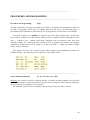
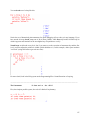
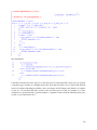
Pi = π the number
pi = π the Greek letter
PI = Π, the capital Greek letter
GAMMA(x) = the gamma function
gamma = the constant .577 (Euler constant),
Gamma = Γ, capital letter
alpha, beta, delta, gamma, epsilon, zeta(ζ), eta, theta, iota, kappa, lambda, mu
nu, xi(ξ), omicron, pi, rho, sigma, tau, upsilon, phi, chi, psi, omega
If you want to use gamma as an ordinary Greek letter, you have to "unprotect it" :
If you want a primed variable like x', enter it as `x'` . Unfortunately `nu'` does not appear as ν' .
nu1 does come out as ν1, however.
___________________________________________________________________________________
Constants :
false gamma infinity true Catalan FAIL Pi I
Recall from the Greek letters discussion that Maple accepts kappa for κ and pi for π and alpha for α.
Therefore, the lower-case pi is just π, a Greek letter (very "inert"). And PI is Π, the capital Greek letter.
Neither of these has anything to do with 3.14159. The correct Maple symbol for that constant is Pi. From
the help: "E is no longer a reserved name in Maple. It has been replaced with exp(1)." The only reserved
constants are: <false gamma infinity true Catalan FAIL Pi>. gamma γ is the Euler–Mascheroni
constant which appears lots of places including as γ = – Γ'(1) ≈ .57. Catalan is a similar constant ≈ .915.
The last item I is in fact not a built-in constant, but is a built-in alias for sqrt(-1).
__________________________________________________________________
ditto operators
%
%%
%%%
and
%n
As each code line is executed, there is a single result and it exists in a "result buffer" called %. So if you
fail to name a result, you can refer to it as %, known as the "ditto operator". The previously computed
result is saved as %%, and the third previously computed one as %%%. Here is an example of % use:
18
So when the plot command is executed, % has the value "sin(x)". If you go off and run some other
commands manually and come back, % will have the value of the last command you ran, not what you
think.
Complex expressions often group messy sub-expressions into items like %1 and %2, and these can be
accessed directly by these names.
A very common use of % is to tack something using it onto the end of a command line":
It is easier to do this than add a whole new command just to see what something really is.
__________________________________________________________________
Inert Forms of Operators
value
Inert operators begin with a capital letter and are often referred to in Maple Help as "placeholders". The
idea is that you defer the evaluation of an operation until you are ready. You do this so you can make sure
you entered your expression correctly (especially complex ones), since it's easier to check it in the typeset
notation. Here are some non-complex examples:
You can convert from inert to evaluated forms using the "value" command, as follows:
// same as diff above
See the "diff" section below for an example where Diff plays a more essential role.
____________________________________________________________________________________
19
____________________________________________________________________________________
macro
alias
macro: These two commands are similar.
A "macro" of the form macro(joe = bob) simply causes the letters joe to replaced by the letters bob
anywhere they appear. Here is an example where we compute P2(0.3) twice:
If we ever want to know what "joe" is macro for, we just type joe; and it tells us. You can use a macro to
make a symbol for any string of letters you get tired of typing,
alias: Here is the LegendreP example done with "alias", and things are a bit more complicated:
First of all, whenever you do an alias, it gives you a list of all existing aliases, and it just happens that the
symbol I is an alias for sqrt(-1) that "comes with" Maple. The way aliases work is basic: in any command
the string joe is converted to string LegendreP and then processing occurs as usual. On output, LegendreP
20
is converted back to joe, so you see joe. There does not seem to be any way to ask Maple what the alias
joe stands for after you create it.
You remove alias joe by saying alias(joe=joe). Several aliases can be put into a single command as in
the example below.
How to replace a default symbol name with another symbol and free up its name
Example: The symbol I by default is -1 . Perhaps you want I to be some electric current, and you want j
to be the symbol for -1 . You first say alias(I=I) which removes the default Maple alias that I stands for
-1 . After doing this, you can use I as a normal variable name. Second, say alias(j=sqrt(-1)) to cause the
symbol j to be -1 . Of course after doing this j cannot be used as a variable name. These can be
combined into the single command alias(I=I, j= sqrt(-1)).
21
___________________________________________________________________________________
EXPRESSION MANIPULATION AND EVALUATION IN MAPLE
__________________________________________________________________________________
type
In a normal computer language, data objects are explicitly "typed" in some way. You might have
something that is a structure that contains three expressions and then 10 3D points, for example. Or you
might have something that is a list, or a polynomial, or a matrix. In Maple, there are many such types, but
they tend to be hidden from sight, and if you want to know the type of some object, you have to ask!
Ultimately, most everything in any Maple structure is going to be a mathematical "expression". A
rational number is a special case of an expression, and an integer is a special case of a rational number.
More generally expressions are things like sin(x) + 2^y.
There are a few exceptions in that some objects can be "strings" of text and a few other things like
that.
Normal languages don't make distinctions like "polynomial" or "numeric", because normal languages
don't process expressions the way Maple does!
It is important for a Maple user to know the nature of his or her objects. If you want to know if object
A is a matrix, you ask Maple as follows:
So no, the number 3.2 is not a matrix. Here is a list of types in Maple, and you see matrix in the list:
22
Notice that list and set are in the list, but sequence is not in the list. In the Help you can click on any of
these items to learn more about it. Maple allows the user to create new types, and there is much more
type technology inside Maple, but that is beyond the scope of this document or my knowledge of Maple.
In the rest of this document, we will often use the type command to learn about an object's type.
__________________________________________________________________________________
Numbers and Base Conversion
Numbers can be integers like 100, fixed point like 100.3, or floating point like 1e3 = 1000. The default of
course is base 10. The number of digits of precision for numbers is 10 by default, but can be set to any
number desired
Math is done in software in Maple so a larger Digits value just slows things down. See evalhf in Maple
help for how to make use of floating point hardware for increased computation speed.
23
Maple can deal with the hexadecimal base 16 as shown in these examples:
Notice that 1E240 is used here as a name and since this name does not begin with a letter, it must always
be surrounded by tick marks when directly entered. If one wants the digits of a number in a list so they
can be processed in some manner, one can say
where notice the least significant digit is first, which is reversed from the normal way digits are displayed.
Also, notice that E = 14 for hex. This last command form works for any base, not just standard bases. It is
possible to take a list of digits in one base and convert it to a list of digits in some other base. In this
example, which uses the lists above, we convert from base 16 to base 10. The second command shows
that it is always easy to get back from a digit list in any base to decimal number (nops = # elem in list)
For octal and binary, the tick marks must not be used in the direct entry. We repeat the above example for
octal (binary works exactly the same way)
24
Warning: One can only convert if one of the bases is decimal. For example, in the first line below the
octal keyword is ignored and the number entered is treated as decimal,
To convert then from octal to hex one must do it in two steps, for example
________________________________________________________________________________
operators
First, here is the list
The usual arithmetic operators are +. –, *, / ; exponentiation is either ^ or **.
Boolean test operators are =, <, >, <=, >= and <> for not equal.
Boolean operators are and, or and not. There is no xor or xnor.
Operators %, %% and %%% are called ditto operators and refer to the last, second last, and third last
item computed.
Operator $ forms a sequence as in these examples (the first two are the same)
Operator ! is the usual factorial operator so n! = factorial(n).
Operator precedence is fairly standard with ^ the highest, then * and /, and finally + and -. But even
higher than these is function argument binding. Some examples are shown here on the left:
25
The usages on the right are legal but seem a bit dangerous.
________________________________________________________________________________
trunc round frac floor ceil mod
From the Help system (comments added)
For x >= 0, trunc(x) is the greatest integer less than or equal to x. For x < 0, trunc(x) = -trunc(-x).
In other words, trunc(x) truncates toward 0, unlike floor which truncates down.
round(x) rounds x to the nearest integer. Round(0.5) = 1 and round(-0.5) = -1.
frac(x) is the fractional part of x, that is, frac(x) = x - trunc(x).
For x ≥ 0, some computer languages use Rem (x) for this function, but not Maple.
floor(x) is the greatest integer less than or equal to x.
For x ≥ 0, some computer languages use Int(x) for this function, but not Maple.
ceil(x) is the smallest integer greater than or equal to x.
x mod m or modp(x,m) is the usual modulo function, m normally a positive integer.
For x ≥ 0, some computer languages use x%m for this function, but not Maple.
For Maple, % is the ditto operator, see above.
________________________________________________________________________________
sequences
lists
sets
seq
repeat operator $
There are three distinct data structure items discussed here: sequence, set, list. In addition, we discuss a
certain operator "seq" which lets us easily build any of these data structures.
A "sequence" is a comma-separated list of expressions, and concatenation works as you would expect.
Here is an example showing the creating of a sequence q, and then a concatenation of the sequence with
more items. We show how you access an element of a sequence using square brackets; the first item in a
sequence is item number 1.
26
We took the liberty of jumping ahead here and made a "list" which is object r, see below. Maple verifies
that r is a list and it is not a set. It cannot say whether it is a sequence, because, although sequences exist
in Maple, they are not a "type", as was noted in the last section. If we want to select a portion of a
sequence we can do it this pretty obvious way:
You can construct a sequence using the seq operator, lots of examples are provided in the help:
If you want a sequence of identical items, here is the easy way using the $ operator (see diff later)
27
A "set" is a sequence surrounded by {....}, and a "list" is a sequence surrounded by [....] . Notice above
that you can use seq to make a set or a list in the obvious manner. Here are more examples,
This shows how to use seq to make a "list" instead of a "sequence". Note that i=1..5 is in fact a "list" as
shown in the first item above.
A "list" has order to it, a "set" has unordered elements or "members". Both lists and sets have
"elements", these are the items. Order versus no order makes a big difference when you do something like
plot a set of points and connect the points with lines to get a smoother curve!
Now here are examples of a sequence, set and list where the members are 2D vectors (points):
In passing, it should be noted that either of the last two objects (the set and the list) can be used to make a
scatter plot of the 2D data using the command pointplot(q) or pointplot(r), see plotting later.
The number of elements in a set or list can be determined using the nops command described
elsewhere in this document. For example, both the set {q} and the list [q] have length 4 :
It is not necessary that all the items in a sequence, set or list be the same type, although the examples
above might give that impression. Here are some examples which use concatenation with the q,r above
28
In the first sequence, there are two items, the first being a set and the second a number. In the second
sequence, there are two items, the first is a list of 2D points, the second is a set of three numbers.
Obviously there is much flexibility in Maple, but certain operations are going require certain data
structures to work properly. For example, you cannot call pointplot(p) where p is a sequence.
Finally, here is an example of a nested structure: At the highest level, we have v which is a list of 2 items.
Each item is itself a list. These secondary lists each have three items in them. The third item is a set of
two lists! Each of those lists has 3 numeric elements. Notice the interesting access v[i][j] which can be
generalized to any level of nesting -- multiple square brackets.
This nested list is pretty handy for showing the eigenvector information of a matrix, you can put all the
interesting information in the same list, and you can access anything you want.
Hopefully the reader is convinced that sequences, lists and sets provide at least all the flexibility that one
might have using C structures in the C language, or C classes in the C++ language (since expressions can
be functions as well as data).
Conversion between Sequences, Sets, Lists, and Arrays
1. Conversion from Set to Sequence and back to Set
29
2. Conversion from List to Sequence and back to List
3. Conversion from List to Set and back to List. Note how this filters out duplicate items.
4. Convert from Array to List and back to Array.
________________________________________________________________________________
30
list
// revisited: doing math with elements of a list
Consider this sample code where we create a list of 5 lists:
Here we create a list of five 3D "vectors", filling them with some dummy data. We display one of the
vectors. We cannot access r[6] because it does not exist. We ask if r[3] is really a vector, and Maple says
no. The word 'vector' refers to something we shall see later which is a "Maple vector". Our object r[3]
does not pass muster to be a Maple vector, it is only a "list", but it can do certain things that a real Maple
vector can do:
We then set new data into two vectors of the list, and proceed to add these two vectors, and multiply a
vector by a scalar, both successful actions. We hopefully try a pairwise multiplication, but this produces a
mysterious object that does not seem useful. In the next line we try computing a dot product pretending
31
that we do have Maple vectors, using a method shown below, and it works! Our next attempted action
with the sine is rejected, so must be done "in longhand" as the next line shows.
The point here is that certain basic mathematical operations can be performed on list elements which
are compatible with each other. Basically, we can add, subtract, and multiply by scalars.
We could if we wanted repeat all the above with true Maple vectors. Here we comment out the first line
with a # to allow easy comparison,
So now r[3] is a vector and not a list. You cannot tell this fact by staring at the object, you have to use the
type command because a list (of this kind) and a vector look the same. The vector math shows slight
variations, for example
When the objects are real Maple vectors, we have to use evalm to get the addition we want.
________________________________________________________________________________
eval
Eval
evalf
evalhf
Examples:
eval(x^2 + 2, x = a)
// evaluate the expression e "at the point x=a" (one variable)
eval(x^2 + 2*y, [x = a, y=b] )
// if more than one variable, must use the "list notation"
eval(e)
// evaluate expression e through all levels of recursion
eval(e,2)
// evaluate only going back 2 levels of recursion
The last two items are useful when you have a chain of equations a:=b where b:= c and so on. As for the
"evaluation at a point", the substitution is made as specified, then the thing is computed as far as it can be
computed. You cannot combine the x=a and n arguments together.
Example:
32
> f := 5 + x^2;
2
f := 5 + x
> eval(f,x=2);
9
As usual, the inert Eval attempts to defer the evaluation, not meaningful in all cases. Here is an example:
> Eval(int(sin(x),x), x=y);
(-cos(x))|
|x = y
> value(%);
-cos(y)
// see "value" above
Notice that the subs command puts in the thing you want, but does not then evaluate the result. (below)
When you say evalf(something), you are asking for an actual floating point number. And if you are going
for speed, you might use evalhf(something) which makes use of the computer's hardware floating point
capability, but it does not work with Bessel functions! [ Notes TBA on evalhf which does not naturally
exist in Maple. ]
Here is a favorite example where second argument indicates number of decimal places required:
Of course evalf is doing software floating point, so like the Krell power source, it will do however many
places asked of it, such as 500,000. There are memory limitations.
The evalf is usually called internally when you do eval on a function at some random argument
location. But for simple arguments, this does not happen and you have to do it yourself:
If something is running way too slow, you might be able to speed it up using evalhf() which uses the
computer's floating point hardware (double-precision) for floating point calculations. However, some
special function calls like BesselJ don't use this so you might not win.Since Digits = 10 by default, softare
computations produce 10 digits while the double-precision hardware does 64 bits which means about 16
decimal places. For example,
33
It is claimed by some that numerical integration always uses evalhf if Digits is set less than 16 or so, at
least for parts of the integration code that can use the hardware effectively.
____________________________________________________________________
subs
algsubs
Methods of making a substitution in an expression. The first makes a substitution without doing an eval,
the sub just sits in there where you put it.
"The function algsubs performs an algebraic substitution, replacing occurrences of a with b in the
expression f. It is a generalization of the subs command, which only handles syntactic substitution."
You might wonder how subs and eval differ. Here is an example showing that eval "evaluates" all it can
Notice also the different argument order for subs and eval.
Another example fills a gap in Maple's convert capability (cannot convert ln to inverse trig) for Q1(iζ):
_____________________________________________________________________________
34
lhs
rhs
numer
denom
These operators just give quick access to the "left hand side" or "right hand side" of an equation, or to the
"numerator" or "denominator" of a fraction. These same operations can always be done with the more
general op command discussed below. Here are some simple examples:
unprotect
type
reserved words and letters in Maple
Suppose you want to use D as a variable name. If you try to do so, you find that it is a protected symbol,
used for differentiation. But you can remove this use and then use it as you like. For example
Maple has a list of 30 reserved words
but there are also some reserved (or at least special) single letters, a little harder to identify -- you have
to go through the Help system one letter at a time in the topic search. Here are the basic ones
35
C
D
I
O
c
a function used to generate code (on the list in Appendix below)
differential operator: D(sin) = cos
D(sin)(x) = cos(x)
imaginary i
used to mean "order of" in some output displays
used for commutators in the commutat package
Although things like J appear in reference to Bessel function, the Maple name is BesselJ(x).
Here are some other reserved names referring to constants
GAMMA
gamma
Catalan
Pi
Γ
γ
not just a Greek letter, it refers to the "gamma function" Γ(x)
again, is used for Euler's constant .57
another constant
another constant
π
And of course there are lots of reserved names which are official function names, including
GAMMA
Γ
not just a Greek letter, it refers to the "gamma function" Γ(x)
These function names are all shown in the Appendix below. The GAMMA one is special because
normally this would just indicate an upper case Greek letter. This list includes Chi and Psi functions
which are not official Greek letters in Maple since mixed case.
___________________________________________________________________________________
unassign
This just removes an assigned meaning to a symbol, for example
___________________________________________________________________________________
assume
is
about
additionally
Some examples: assume(a >= 0), assume(theta>= 0, theta < Pi), assume(a,real) .
For a given variable, you must put everything into a single assume statement, otherwise the last assume
statement you execute wipes out the results of earlier ones, though this problem can be fixed using the
additionally command. One something is assumed, you can inquire about it using is and about.
36
Once you assume something about a variable, that variable will appear with a tilde suffix in all
subsequent stuff as a reminder. You can turn this off with the Options (recommended).
How do you unassume? There is no "unassume" command. You do this by saying a := 'a'; which
seems strange. Here from the Help: "Assumptions made on names may be erased (cleared) by unassigning names. For example, having assumed that x is positive, x := 'x'; clears this assumption made on
x." (See unassign elsewhere.)
Why would you want to assume something about a variable? One reason is to allow Maple to clear
out square roots and other fractional powers.
Examples:
Maple frequently seems incredibly stupid about canceling things in numerator and denominator as in
these examples. Its reason is that it doesn't know which root you want:
37
y=
x2
=>
y = +x , -x
y = (x3)1/3
=>
y = x , eiπ/3x , e2iπ/3x
You always assume the first root, but Maple has to be more careful to not mislead you.
A second typical use of assume is to make sure integrals converge:
Example:
Maple does not "deduce" all the information a person would given a set of assumed facts, so it is usually
necessary to put in everything but the kitchen sink if you want things to work right. For example, if you
have a situation where 0 < ν < h < μ < k < ρ (which arises in elliptical coordinates), you need to say
Then when things like (ρ-k)2 appear, Maple will know this is ρ-k and not k-ρ, for example.
As noted earlier, you can learn what Maple is assuming about a variable with the about command.
For example, after the above assume we get
38
The "assume facility" as Maple likes to call it has a few unexpected side effects. On the left below
perhaps you assumed B was real for some reason, then later on you assign A := B and after that you
assign B := 2. You might logically expect A to be 2 as this point, but it is not! You try to fix the problem
by "assigning the assumed variable name", but Maple thinks little of that idea: The way to deal with this
problem is shown on the right
I think the real problem illustrated in the above example is that "you cannot assume on a constant", even
if the assumption is true for that constant. Consider first this code:
where the error message indicates the problem. But if we do the assume first and then do the assignment,
as in the previous example, there is no error message and the user is a bit mystified. Maple seems to just
quietly reject the assignment of B to a constant in already-defined expressions which include B.
Here is a real-world example where the eval command makes several replacements at once. The assumes
are done in this case to allow Maple to generate a relatively simple expression for the integral :
39
____________________________________________________________________________________
collect, coeff, normal, simplify, expand, combine, factor, rationalize, convert
These all have their special quirks. I have found that in the end you cannot really make Maple do exactly
what you want in displaying the final results, but you can try these things. Each has its own Help.
collect groups terms by some item you select, a typical case would be
The second argument of collect can be a function as in the following example. Recall that % means "the
last thing computed". Note that it helps to "expand" before "collecting" to get the simplest result :
40
The last command coeff shows how to "pick off" a desired coefficient.
One can "collect" in terms of multiple variables in different ways. In the example below, f is a polynomial
of degree 2 in x and y. You might want to just see this polynomial "as is" with like terms grouped
(distributed option), or you might instead like to see it collected first on x and secondarily on y. Both
ways are possible:
normal puts things where possible into a ratio of factored expressions, for example.
41
simplify uses things like trig rules to attempt to simplify an expression, and also combines terms and does
obvious algebra things a human would do. Here is an example from real code which first displays a
matrix in a messy form (as four row vectors), and then simplify gets things under control.
Sometimes simplify will "unsimplify" something you have done earlier, like a collect operation.
See section below "Frustration with Simplification" .
expand and combine work in opposite directions, but results are not always what you expect:
Combine has many options encouraging the use of knowledge of some set of rules, see Help. Here is a
simple example:
42
factor seems pretty smart in general.
rationalize gets rid of square roots in denominators, a very simple example being:
convert has many operating modes depending on its second argument, which can take all these values:
Note that trig includes trig and hyperbolic functions and you cannot force one or the other. Newer Maple
adds trigh to the above list to force conversion into hyperbolics (although Maple V.5 does have the type
trigh). Often the command combine(f,trig) will do the trick (combine expands things like sin(a+b) ).
Example: This shows the use of the combine command just mentioned.
43
Example: Here we use Bateman v1, p 132(37) to evaluate the Q1(z) function using "standard functions":
Example: partial fractions
___________________________________________________________________________________
operands
nops(s)
op(3,s)
An operand is one of the items acted upon by operators at top level in a Maple expression. If top level is
a function, then the arguments of the function are operands. Function nops(s) tells you how many
operands there are in an expression (at top level), and op lets you pick out one of these operands.
44
If you want to get a list of all the operands Maple thinks there are in an expression, do op(s). Using this
op notation, you can dig down into a very complex Maple expression and extract any sub-expression you
want. You just do it recursively: a = op(2,s); b = op(7,a); and so on.
Suppressing function arguments
Example 1: Sometimes it is necessary to display arguments of a function to make things "work right", but
then in the result one might prefer not to see the arguments. Consider:
When the undefined function f has no explicit arguments, the deferred Diff differentiations activated by
the value statement give the result 0 since Maple assumes f is a constant. This is repaired by changing f to
f(x,y). If expressions are long and/or there are many arguments, it might be desirable to suppress these
arguments in a final result, and the above shows one way to do this by extracting the function name using
the op command. See elsewhere in this document for comments on Diff, value, % and subs.
Example 2: This fancier example illustrates several things at once: how to get nice subscripts on a vector
function, how to tell Maple not to throw out derivatives of unknown functions, and how to get Maple to
suppress function arguments after they have been explicitly added. It is the suppression of the arguments
that involves the "op" command which is used below to "pick off" just the function name as op 0, causing
the arguments of the function to go away, as in the previous example. Things are very delicate because
Maple always wants to compute derivatives of things which it often interprets as constants. One
constantly has to tell Maple to "defer" evaluation by various methods. One is by using Diff instead of diff
45
when Diff occurs perhaps in a sum structure. Another is by putting apostrophes around the subs command
shown below (another example of doing this appears in Example 5 of the Procedures section below).
So, consider the following piece of code which generates an expression for a variable q (the bulk of
the code has been snipped away). The three functions Br, Bθ and Bφ are never specified, they are just
some generic functions of the variables (r,θ,φ).
.........
The object q is generated by expressions such as the following,
Diff(Bp[2](xp[1],xp[2],xp[3]),xp[2])
meaning ∂θBθ(r,θ,φ) ,
where the three arguments of Bθ are explicitly shown to prevent Maple from thinking Bθ is a constant
with respect to any of the arguments. Once the object q has been computed, one might like to suppress all
the arguments since they clutter up the expression. This seemingly trivial task can be done by the
following additional code:
The result is for display purposes only. It is unstable in the sense that if it is "evaluated", the last three
terms vanish because Maple thinks the last three derivatives vanish, as shown in the next code line,
46
Frustration with Simplification
One frustration in using Maple is that it often has trouble simplifying the individual terms in a sum of
complicated terms. Here is a example showing a work-around that sometimes helps:
Here no amount of bashing on expression f with operations like "simplify(f)" will reduce it to π (unless
you have a "lucky run" based on random internal ordering of things). Maple does not realize for example
that it can cancel sinθ even though the assume guarantees an unambigious root. The code loop expands
expression f into a sum of two terms and then simplifies those terms one at a time and constructs a new
expression as the sum of those simplified terms. In this way, we discover that the integral equals π. Here
is the text for the above example, paste it into a worksheet and it will run:
restart;
assume(theta>0,theta<Pi);
Int(sin(x)/(sqrt(1-cos(x))*sqrt(cos(x)-cos(theta))),x=0..theta);
f := int(sin(x)/(sqrt(1-cos(x))*sqrt(cos(x)-cos(theta))),x=0..theta);
acc := 0:
f1 := expand(f):
for n from 1 to nops(f1) do
t[n] := simplify(op(n,f1)):
acc := acc + t[n];
od:
f2 := acc;
Algebra with complex numbers
evalc
Maple assumes variables are complex, so if one wants them to be real, one must say so. Consider for
example,
47
Maple understands our intention that a,b,c,d are supposed to be real numbers, but it is still a bit
recalcitrant in doing things. It easily finds the value of |z|2 , but balks at computing Re(z). This problem is
remedied by the evalc command:
Here is another example :
48
Algebra with trig functions
subs
Maple sometimes does not do what you would normally do. Consider
You might like to see sin2(x) in the denominator, but Maple sees no need to do that. So you have to tell
Maple to do this "manually" :
Here is an example combining methods of the last two sections:
49
___________________________________________________________________________________
NON MATRIX RELATED MATH FUNCTIONS/OPERATIONS
___________________________________________________________________________________
How to Define a Function of Arguments
(1) the mapping operator " ->"
user defined functions
Here are two ways to do the same thing:
If you want to evaluate something by putting an argument like f(x), then you have to use the "mapping"
method as shown on the right, and include the argument when plotting. You can do multiple variables for
example
g := (x,y) -> sin(x)*cos(y) + x*y;
The arrow object -> has a little man page in Programming/Procedures and Functions, first item.
In Maple, a function is a function of a list of variables (arguments). I don't think you can define functions
of more complicated objects, such as a function f(r) where r is a vector. You can of course do f(x,y,z)
with three scalar arguments.
50
Difference between built-in functions and user-defined functions.
In Maple, a built-in function like sin(x) behaves as if the function name sin were "unassigned". Consider:
Here joe is something we just made up and of course Maple has no special knowledge of joe. It goes have
a lot of knowledge about sin in different ways. For example, it knows how to evaluate sin(1) as shown on
the right above. Note that sin(x) and joe(x) are both of type "function". If we now assign joe to be a user
defined function using -> (or unapply), joe is no longer "unassigned" and joe(x) ceases to be of type
"function". Here is a little comparison:
Both sin and joe are procedures, but joe is an operator while sin is not an operator. We just point out this
technical difference without trying to explain it. It is not clear how one would create a user-defined
function that had exactly the same type properties of a built-in function. Technically, Maple regards a
function like joe as a "functional operator". Both joe and sin are ultimately "procedures" (see elsewhere in
this doc).
51
(2) unapply
use to "functionalize" an existing expression
The name of this command is fairly obscure, but it can do something extremely useful. Suppose you have
a long series of manipulations that create a complex expression "f" and in this expression the variables x
and y happen to appear. You would like this thing to magically become a function F(x,y) so you can
conveniently compute F(3,5), say. How do you do that? In other words, how to you create a function
(which is a procedure call) in Maple if all you have is an expression?
The following method does not work:
You want F(2) to be sin(2), not sin(x). As in the previous example above, if you type sin(x) to the right of
the arrow, it does do what you want, but if you already have sin(x) sitting in an expression f, it does not
work. The unapply command comes to the rescue:
Here is a two variable example which better fits our original statement of the conundrum:
Unapply "unapplies" all the arguments so you can "apply" them later.
52
(3) unapply
used to create the derivative of a function
Here is a famous application of the unapply idea. Suppose you want to make a Maple function which is
the derivative of another function. You might dimly start out like this:
The problem is that x is set to 2, then it tries to compute diff(f,2) which makes no sense. We want to
compute the derivative first, and THEN set x = 2. We want to "unapply" this x thing and get it in there at
a later time. Here is one way to do it:
Here is another way to do it, where we first make f be a true function of x, not just an expression which
includes x. In this case, notice that we put f(x) and not just f as the first argument of diff.
Maple has this notion built in to its D operator, and you get the same result more quickly this way
The thing D(f) is a function, like sin is a function, and then the argument is 3, as in sin(3). See
differentiation for multiple variables and partial derivatives.
___________________________________________________________________________________
53
fsolve
Suppose you want to know where two curves intersect,
It solves for a value of the second argument which makes the first argument be 0. The search range of the
second argument is given in the third argument. Once it finds one root, it stops, so you might have to
provide your own range to get another root. Probably it is doing Newton iteration, the f in fsolve.
________________________________________________________________________________
solve
variables which are "equations"
M equations in M unknowns
You can of course do this in the matrix sense of Ax=b using linsolve discussed in the matrix section
below. Here is another way to do it, by example. We are solving four linear equations in 4 unknowns
here. Notice in the first four lines that you can define a variable to "be" an equation. This is a little
unusual for normal programming languages. This is where "=" is used in Maple, as opposed to ":=".
Notice that the solutions p,q,r,x cannot be accessed by Maple until the assign(S) statement has been
executed as shown above. This goes through the sequence of solutions and converts each solution into an
assign statement. Prior to this p,q,r,x are just "text".
54
Here is an example using a directly stated equation,
On the other hand, if you just put an expression, it solves the equation expression = 0 (ie, roots)
Two meanings of _Z : (1) dummy in RootOf; (2) "any integer"
Solutions that solve comes up with sometimes contain the RootOf operator with its _Z variable, which is
a bit confusing. Here is some sample code showing what this means:
The symbol _Z is just a dummy variable like x in the equation ax2+bx+c = 0. In general if we have f =
RootOf( g(_Z)), that means f = _Z = a root of g(_Z) = 0. For some reason, Maple does not actually solve
for the root unless you force it to, as in the second command above. For polynomials of degree 5 and
higher, neither humans nor Maple can find analytic roots. Maple can do some degree 4 if you are lucky.
The second use of _Z is illustrated in this example which illustrates several things at once:
55
Remember this is Maple V. Maple is unable to solve the equation fd1 = 0, but when it is advised to use
simple trig identities by the combine stastement, then it can solve the equation as shown. Then when the
1
_EnvAllSolutions variable is turned on, it adds 2 π_Z to the solution. (If the option to add tildes to the
1
end of "assumed variables" is turned on , this appears as 2 π_Z~) . It means (π/2)*N where N is any
integer, so here _Z is sort of representing the field of integers, Z being a standard symbol for that use.
Notice that this use of _Z is completely unrelated to the dummy variable usage above. In our example, the
reason for adding (π/2)*N is that if 2w = tan-1(z) gives a solution w, then 2w+Nπ is also a solution,
1
1
which then means that w + (π/2)N is also a solution. In newer Maple, one might see 2 π_Z1~ or 2 π_Z2~
and so on, to allow for multiple different arbitrary integers. Also, one can say
solve(fd1m=0,x,allsolutions=true) to set the env variable shown, but in Maple V you must do that as
shown above.
________________________________________________________________________________
dsolve
solving differential equations
The dsolve command can solve ODE's (and systems of ODE's) of any order, and it can do so either
analytically (though it may not succeed) or numerically. The ODE's need not be linear ODE's. There are
many features and options in this large sub-world of Maple, see Help. Maple has a separate command
pdsolve for finding analytic (but not numerical) solutions to PDE's. We are talking Maple V here and no
doubt both these worlds have expanded. Below we do three examples first analytically, then we repeat
them numerically. The examples are a first-order ODE, a second-order ODE, and a system of 2 ODE's. A
final numerical Example 4 shows how to use dsolve to plot magnetic field lines.
ANALYTIC
Example 1. In our first basic example, we specify an ODE and then have Maple solve it,
Integration constants begin with an underbar as for _C1 shown. There is no mechanism for stating a
boundary condition in this form of the dsolve command. If you happen to omit the = 0 from eq1, then eq1
is an expression instead of an equation, but the dsolve call then adds the = 0 for you, assuming that is
what you meant.
The object f is not an expression, it is an equation, just as object eq1 is an equation. We can obtain the
right side of the equation f by picking off the second operand as follows,
56
Perhaps more usefully, we would like to have u(x) be a function of x, so instead of the above command
we could do this (see elsewhere in this document for "unapply"),
To plot the solution, we set in a value for the constant, and plot away,
Example 2: 2nd order
and see above for how to pick off the function u(x). Now there are two integration constants.
57
Example 3: A system
The output "f" of the dsolve command is now a set (recall that {...} means a set) of two equations. In the
command itself we specified a set of two equations which comprise the system to be solved, followed by
a set of the functions we want Maple to solve for. As before, we extract functions x(t) and y(t) ,
At this point we could set in some constants and do a plot,
58
NUMERICAL
If Maple cannot find an analytic solution to your ODE or system of ODE's, it can generate a numeric
solution without too much trouble. We shall repeat the above examples numerically.
Example 1 (numeric)
The first step is to "make the call" :
Here we use "some other symbol" (namely U) for the function name, so we can safely use u(x) as
described below. Notice that the equation and boundary condition(s) appear in the first set {...}, while the
function(s) you want to know about appear in the second set. The type=numeric of course instructs Maple
to do a numerical solution, and the output= item tells Maple to present its solution as a "list of
procedures". Actually, what you get is a list of two equations. The second equation says that dsolve has
created some procedure called U(x) which evaluates the solution of our ODE at some point x. The first
equation is a sort of identity procedure x which we won't worry about. Since this is a numeric solution,
one might visualize the first dummy procedure "x" as providing the x values and the second procedure
"U" as providing the y values for a plot of the solution.
We can take a quick look at some value of x, and do a fast plot as well using the special odeplot call,
where [x,U(x)] specifies the two axes of the desired plot. The actual solution U(x) is a procedure which
probably has a set of constants for the solution and interpolates them in some reasonable fashion to
provide the illusion of a continuous solution.
But if you want to use this solution, you have to jump through another hoop which is this (where we
now arrive at the desired u(x) object) ( rhs means to extract the right hand side of an equation)
59
Now we can evaluate u(x) for any x, and we confirm the boundary condition in the last line.
Just for fun, we can examine the pedigree of u,
This is the same as the pedigree of sin as discussed in the -> operator section. The reason we have to add
the single quotes in the first line is that this function does not have the little protective "wrapper" to repair
a certain "first time called" problem. This is discussed in our section on Procedures, Example 4. We could
add the wrapper which tests "if type(x,numeric)" as shown there, or we can just use the single quotes to
delay evaluation one time and the problem is fixed. Here is another example where the single quotes are
needed for this same reason (the function is probed at the start without a numeric argument and this kicks
out an error)
Here is the wrapper fix just for the record:
60
I think this little issue has been repaired in later versions of Maple.
If you want the derivative of u(x), you cannot just use diff(u(x),x) or diff('u(x)',x) because u(x) is not an
expression which can be differentiated, it is really a procedure call. One solution is to reformulate the
ODE and solve it for the derivative (which in this example happens to be trivial). Another way is to just
roll your own approximate derivative,
In the next example, dsolve provides both the function and the derivative since it involves a 2nd order
ODE.
Example 2 (numeric)
First we have the call to dsolve,
The new feature here is that there are now two boundary conditions required, and they both go into the set
with the equation as shown. Instead of saying u'(0) = 2, we write D(u)(0) = 2 or (D@@1)(u)(0) = 2. For a
third-order ODE, one would specify a third boundary condition as (D@@2)(u)(0) = 0 and it goes into the
set as well. For a quick sample point and a quick plot,
61
We can "extract" the function u(x) as in the previous example,
The first derivative can be similarly extracted,
Example 3 (numeric) A system
The call is
Notice that the two boundary conditions are in the first set with the two equations. Extraction of the
functions x(t) and y(t) proceeds as before,
62
Sometimes one sees the extraction done slightly differently,
The results are clearly just the same, but the advantage is that you don't have to know the number of the
equation in list f where your function of interest resides. In the subs syntax, the first item here is a list of
three replacement expressions while the second item is the object into which those substitutions are made.
So two of the substitutions in list f do nothing, while one replaces X(t) by proc(t) ... end (for example).
We now have several odeplot choices:
63
Alternatively, we can use the usual plotting routines instead, bearing in mind the first-time issue requiring
the quotes just discussed in the numeric Example 1 above:
Example 4 (numerical)
Another system of two ODE's
Here is a real-world use of dsolve to plot magnetic field lines for two parallel cylinders each carrying a
uniform current density and having radii a1 and a2 and center separation b. We do not give an
explanation here, but just present the code as a useful example of dsolve solving a simple ODE system.
This code runs much faster than an iterative tangent tracking routine with the similar accuracy. That kind
of routine does r(n+1) = r(n) + δ [H(n)] / | H(n) | with δ some small value.
64
________________________________________________________________________________
65
rsolve
solving difference equations (recursion equations)
Example: Given Xk+1 = aXk + p with p = (1-a)/2 and X0 = 0, solve for Xk:
Example: Given on+1 = - a on + b in with o0 = c, solve for on where in is some unspecified sequence.
This example shows how to cause the solution to be a function of n, and provides examples of the
following other Maple functions, all discussed in this document: subs, unapply, value.
If the subs step is not done, o(4) turns n0 which is n[0] into 40 which is 4[0]. The result comes out the
same at the end, but it just looks a bit odd with 4[0] as the summation variable. As one can see by
displaying the output in "Maple notation" instead of "Typeset notation", the sum in the o(4) line above is
the inert Sum function. This is then executed when value is applied. We could have used i(n) in place of
i[n] in the original rsolve line, then the output involves i(0), i(1) and so on.
_____________________________________________________________________________________
66
sum and add
product and mul
Use sum or product for symbolic, use add or mul for numeric. Add works with evalfh, sum does not.
Anything here can be an expression. See Help for discussion of putting things in single quotes.
___________________________________________________________________________________
Integration
int Int
Here are some examples where we include the inert form at the start, then indefinite, then definite. On the
right is an example of a double integral.
If you want to force a numerical integration, use evalf(Int...). Here is an example where the expected
result is 0, but we use some extra arguments to make the integration go faster (see Help). Notice that the
first attempt without evalf just returns a statement of the desired integral.
As just noted, Maple can do multiple variable integrations. This example illustrates a few more facts:
67
For the first red command line, the inert Int is used, so we just get a statement of the integral. In this
statement, notice that the integral signs with their endpoints are in the same order as the differentials. The
second command line value(%) [ recall % is the last computed quantity ] causes the inert Int's to become
active int's and then the integral is performed analytically as shown. The third red line just expands this
into a sum of terms for comparison with the output of the fourth red line. Using value(%) is easier than
rewriting the integral using int's as shown on this fourth red line. On the third last line we evaluate the
analytic integral to see its numeric value. The second last line forces Maple to do a numerical calculation
of the triple integral to an accuracy set by the global Digits parameter (10). The last line indicates that
only 5 digits of accurate are required so the numerical integration is then much faster. Notice the close
agreement between the analytic and numerical results at 10 decimal places.
Maple can do contour integrations in the following sense. Consider this example,
f(z)
{ dz
J=∫
(z-a)(z-b)2 = 2πi Σresidues
f(z)
q = (z-a)(z-b)2
where we assume that f(z) is analytic within the contour and that poles a and b are located within the
contour. The Maple calculation is then
68
Here we first compute the integral for arbitrary numerator function f(z), then we select f(z) = e5z to get
the integral for that case. Maple's contribution here is the residue command. This method of course does
not work if f(z) has a branch point within the contour, in which case it is not analytic inside the contour.
If the denominator is not in factored form, other Maple tools can help, for example:
____________________________________________________________________________
69
Differentiation
diff
Diff D
This opening barrage of examples shows how to do ordinary and partial derivatives.
The second item is just a reminder that the $n operator creates a sequence of identical entries.
Recall that Diff is the inert form of diff, which means it does not evaluate until told to do so by the value
operator,
The following example shows a situation where using Diff is absolutely essential. Matrix S just provides
data for the example. The next two lines show that diff(S[a,a],θ) = 0 because S[a,a] = Sa,a is a constant
since a is undefined at this point. In the next line A := sum(diff(S[a,a],theta),a=1..3) the diff is executed
first because it is in the innermost expression, and one gets diff(S[a,a],theta) = 0 for the reason just
explained, so the sum is the sum of three zeros. We need to defer the diff operation until after the sum has
been expanded so diff will then act on something like S[1,2] which is in fact a function of θ. That deferral
is provided by using Diff in the second command A := sum(Diff(S[a,a],theta),a=1..3). Since sum is lower
case, the sum is carried out and then assigned to A. Then the final value command causes the Diff to
execute.
70
The D operator (see unapply discussion earlier) can provide higher derivatives as follows:
If we don't specify a function f, it is easier to see what is going on:
Here are examples which involve partial derivatives
71
The object D[1](f) is ∂f/∂x because x is the first argument in the argument list of f . The objects shown
above are ∂xf, ∂yf, ∂x∂yf, ∂x2∂yf, [∂x2∂yf](1,2). I don't think there is a way to combine the @@ notation
with the partial derivatives, so you have to build up higher derivatives manually as shown. We repeat the
above with no function defined
The Help page on D has yet more to say, but we have given the main ideas here.
_________________________________________________________________________________
72
piecewise and periodic functions
Here is an example of a piecewise function:
It is really like a little "case" statement. The rightmost argument is the default if x is in none of the ranges
which you specify, which in our example is when x<0 or x>1/2. You can symbolically or numerically
integrate a piecewise function using the usual int command.
It is sometimes useful to construct a custom function like the above and then make it be a periodic
function across the real axis. That can be done like so:
where the argument of f(x) maps integer ranges of the real axis to the interval (0,1),
_________________________________________________________________________________
73
Integral and Series Transforms
Maple is aware of the following integral transforms, which require with(inttrans):
Calls are provided for Fourier, Hilbert, Mellin and Laplace transforms and their inverses. The Fourier
Sine, Fourier Cosine and Hankel transforms are their own inverses. There are also routines for the Z
transform (ztrans, invztrans) and FFT (FFT, iFFT). The add and save table items allow the user to
enlarge the internal transform lookup tables. Here is an example of a Laplace Transform, where one
should note carefully the ordering of the last two arguments:
Series transforms like the Fourier Series Transform are done "manually" in Maple using an integral to
compute coefficients and then the sum function to add up some number of terms. For f(x) = x on the
interval (-1,1) for example we can write
_________________________________________________________________________________
74
dchange
doing PDE work with coordinate transformations
The dchange package does many things, here is a simple useful example. First, one can manually
compute the following facts concerning how ∂x and ∂y are expressed in polar coordinates,
∂x = cosθ ∂r - (sinθ/r)∂θ
∂y = sinθ ∂r + (cosθ/r)∂θ
.
Here is how to make Maple obtain this result:
The transformation of interest (in this case, Cartesian to polar coordinates) is first installed in a set {...}
called tr (for transformation). The dchange command is told about this transformation, and is given some
partial differential expression as its second argument, and that expression is converted to a partial
differential expression in the transformed coordinates. As one does by hand, Maple just uses the chain
rule to obtain the result.
series
series expansions about a point
A few examples show the basic idea. First argument is function to expand, second the point about which
to expand, third is number of terms.
75
________________________________________________________________________________
Differential Operators: curl
diverge
grad
laplacian
vector Laplacian
For some reason Maple V decided to use "diverge" instead of "div" for divergence. Perhaps div suggests
"divide" though div is not a reserved word. First, here are some 3D Cartesian examples:
But Maple can do all these things in any many different coordinate systems, not just Cartesians, and not
just the 11 classical systems like spherical and cylindrical and ellipsoidal. Here is the list:
At present, Maple supports the following coordinate systems:
In three dimensions - bipolarcylindrical, bispherical, cardioidal, cardioidcylindrical, casscylindrical, confocalellip,
confocalparab, conical, cylindrical, ellcylindrical, ellipsoidal, hypercylindrical, invcasscylindrical, invellcylindrical,
invoblspheroidal, invprospheroidal, logcoshcylindrical, logcylindrical, maxwellcylindrical, oblatespheroidal,
paraboloidal, paraboloidal2, paracylindrical, prolatespheroidal, rectangular, rosecylindrical, sixsphere, spherical,
tangentcylindrical, tangentsphere, and toroidal.
In two dimensions - bipolar, cardioid, cassinian, cartesian, elliptic, hyperbolic, invcassinian, invelliptic, logarithmic,
logcosh, maxwell, parabolic, polar, rose, and tangent.
76
And here is a simple example showing how the coordinate system is specified:
Maple assumes a specific ordering of the curvilinear coordinates, which in the above example is r,θ,φ.
The Maple orderings are stated in the Help system for each coordinate system, along with the equations
which define the coordinate system. All systems assume the order [u,v,w], and then for example,
spherical:
x = u*cos(v)*sin(w)
y = u*sin(v)*sin(w)
z = u*cos(w)
from which one can see that u,v,w = r,θ,φ in the usual notation.
If the above list of coordinate systems is not enough, you can add your own user coordinate system using
the addcoords command (which of course is how Maple constructed the above list).
If you just want to see what a certain differential operator looks like in a certain coordinate system, follow
this example which uses an unspecified scalar function g(r,θ,φ) and vector function T(r,θ,φ) :
77
where in the last command we have expanded each component on r to get a convential result.
The vector Laplacian can be obtained from (@ is Moon and Spencer notation)
@ B ≡ grad(diverge B) – curl (curl B) = " ∇2 B "
Recall that [@B]i =∇2[Bi] only in Cartesian coordinates, where ∇2 is the scalar Laplacian.
The reader interested in learning how Maple computes all these curvilinear coordinate expressions will
find the answer in our document "Tensor Analysis and Curvilinear Coordinates".
78
________________________________________________________________________________
MATRIX/VECTOR RELATED MATH FUNCTIONS/OPERATIONS
_________________________________________________________________________________
The batting order for this section is this: we first mention briefly the notion of a table, and then talk about
the arrays. The 1D and 2D array structures are also known as Maple vectors and Maple matrices. Then
finally toward the end we discuss the slightly different vector and matrix notions which are part of the
linear algebra library (package) called linalg.
___________________________________________________________________________________
table
A table is a one-dimensional list of items each of which has a key. Here is the example Maple gives,
A table is used to look things up, so here you are perhaps looking up the derivatives of two trig functions,
at least in terms of the function name. Accessing a table entry uses square brackets around the key.
If you don't specify a key, it assumes the keys are 1,2.... (such a key is called "an index")
Notice that the table command allows you to fill in some entries right in the command itself (an
initialization list), although you can also add things at a later time,
79
___________________________________________________________________________________
array
Here is our first example which shows a 1 dimensional array which gets initialized in the array command
Maple recognizes P as a table, an array, and a vector, but it is not a matrix. It is also not a "list", but it
looks exactly like a list when it is displayed as by the print command above. Accessing an element again
is with square brackets.
If one says
col := [red,blue,green];
then col is an array and by default it has legal indices 1,2,3 and col[1] = red. If some other indexing
choice is desired, it must be explicitly stated, such as
col := array(0..2,[red,blue,green]):
and then col[0] = red. Any integers are allowed for array indices.
Here is a little code showing how such a 1D array could be used
80
Now let's try a 2 dimensional array
Notice first how the data gets initialized: it is a list of two items, each of which is a list of two items. The
second line shows element access, while the third shows Maple can do matrix multiplication on such 2D
arrays using the evalm command and using the special symbol &*. The last line shows that the symbol *
is reserved to multiply a matrix by a constant. Maple recognizes the array P as a table, array, AND a
matrix.
Next, we might as well throw in a 3 dimensional array:
81
The data initializer list is now a list of two items, each being a list of two items, each of those being a list
of two items. Maple recognizes this thing as a table and an array, but not a matrix or vector.
I presume Maple can handle as many array dimensions as the user needs.
The elements of an array need not be the same type of object. Consider,
Note: Reference to an element of an array requires that all array indices be specified.
How to work with a long list of vectors
Imagine you have 1000 points of the form (x,y,z) and you want to store them in a reasonable manner so
you can work with them as vectors.
1. One way is to have this list of vectors be a 2D array. This method is extremely inconvenient because
everything then has to be done with individual vector components, since all array indices must be
specified.
82
You would like to say a[2] := [4,7,11] for the last line, but a[2] is illegal.
2. An alternative is to store the points as a sequence of vectors, where one gets the possible benefit of
initializing the vectors to desired values :
The problem here is that, although a[2] is understood by Maple, it cannot be assigned.
3. Next, we can slightly upgrade the above idea by making a be a list instead of a sequence.
This approach works, but the Catch 22 is that it does not work if the sequence has more than 100
elements!
83
4. Here we store the points as an array of lists so each vector is a list of three elements:
Although array elements can all be different types, we have in the second command initialized each
element of the array a to be a list of three elements which we think of as a vector, though in Maple the
type is list, not vector. So storing a large number of 3D vectors as an array of lists seems to solve the
problem. This avoids having a "long list" which Maple complained about in item 3 above.
As shown above, Maple will add the elements of two lists of the same size. Maple will not do
component-wise addition of two items which are of different type, such as adding a list to an array,
84
Since A is an array, its elements must be accessed by an index. When A and B are "printed", they both
look like lists, but only B is a list and A is an array. If in the above code one were to omit the declaration
of A as an array, then A is interpreted as a table, and again the addition fails.
___________________________________________________________________________________
matrix
"matrix vectors"
evalm
Here is the same matrix built three different ways:
Key Fact: There is no distinction between a matrix and a two-dimensional array.
Matrix Vectors.
If a matrix has one row or one column, we shall call it a "matrix vector" (a linalg vector) which is just a
special case of a matrix. As we shall see below, there is another animal called a "Maple vector" which is
not the same thing. The keyword "vector" in Maple always refers to this Maple vector object. So consider
85
Notice that, in the matrix R = [a b] above, there is no comma separating the elements. The last two lines
show the expected results of contracting a row and a column vector with the row vector first on the left,
and then on the right. The first is the dot product of the vectors, the second is a new matrix. The operator
evalm is discussed just below.
Math with Matrices
Conforming matrices can be added or subtracted with the usual + and - operators. The * operator is used
to multiply a matrix by a scalar, while the operator &* is used to multiply two conforming matrices.
Square matrices can be raised to a power with the usual ^ operator, as in A^3.
Evalm
Recall the way the operator evalf is used to evaluate an expression to a floating point result:
It a similar fashion, the operator evalm (evaluate matrix) is required to evaluate a matrix expression to get
a result:
86
Matrices which do not "conform" properly generate an error message upon evaluation, as one would
expect:
The zero matrix and the identity matrix in evaluation
In matrix evaluation, any matrix filled with zeros can be represented by the symbol 0.
Any identity matrix (diagonal of 1's) can be represented by the four-characters &*() .
In the first line we add our 0 matrix causing no change. In the second, we right-multiply our matrix shown
by an implied 3x3 identity matrix to get back the original matrix. In the last line we left-multiply the
matrix Q by an implied 2x2 matrix of 0's and the result is a 3x2 matrix of zeros represented just as 0. One
87
might wonder why one would do any of the three operations. We shall see a reason below in our
"unexpected behavior" subsection.
Stand-alone zero matrix and identity matrix.
Here are fast ways to create these matrices,
where recall that 0$3 generates 0,0,0, $ being the repeat operator.
Creating a matrix from a function f(i,j). First, an example from the linalg[matrix] info page,
This very simple example verifies that, for a matrix constructed in this manner, the matrix displayed is
Tij, which is to say, i is the row index, as you would expect from the notation.
Here is another example showing the construction of a matrix Tup which is the transformation matrix
which connects Cartesian to Spherical coordinates. The main point of this example is to show how easy it
is in Maple to build an important matrix.
88
The rows of Tup are the so-called tangent base vectors. Using the linalg transpose routine discussed
below, one can then compute the metric tensor gup = Tup TupT for spherical coordinates, which comes
out being
Creating a matrix from a function f(i,j) using inert operators
In this example, 2x2 matrices U and D (D was unprotected then unassigned!) and column vector h were
predefined. The 2x2 matrix P is constructed where each entry is a double sum involving a derivative. The
variables q1,2 have been preset to r and θ. The inert forms Sum and Diff have been used to cause deferral
of their execution. If one uses sum and diff instead, matrix P comes out all zeros. The double for loop
then causes each symbolic entry of matrix P to be evaluated using the value(..) command, at which time
Diff and Sum are executed. The results are put into matrix X which is then displayed. The value
command cannot simply be applied to matrix P. (See item below concerning when elements of matrices
are evaluated. )
Empty matrix. The call matrix(m,n) creates an m by n matrix with unspecified elements.
89
Displaying a Matrix: Unexpected Behaviors. A matrix is a storage bin for expressions. The matrix
elements are expressions just as are the non-matrix variables of Maple. Let's define the following matrix:
The first perhaps unexpected behavior is that after you have created matrix V, when you type "V; " you
might expect to see the matrix you just made, but all you see is "V", as if V had never been defined to be
anything at all. But the next line V[1,2] shows that Maple really does know what V is, and confirms that
the first index is the row index. If you want to "see" the matrix, use either print or eval as shown.
Now, suppose we set variable k = 4. Look what happens
So the second unexpected behavior is that, after we set k =4, we expect that when we display the matrix
whose elements are functions of k, those expressions will be evaluated with k = 4, but all we see is the
original matrix unevaluated. Compare this to what happens at the top level in Maple
90
The object "f" really is the expression -3*k all the time. If we set k to some number, that fact is not
changed. The difference is that when we type "f", we see the expression "evaluated", whereas in the
matrix case we don't see it evaluated.
If you want to force Maple to evaluate the elements of a matrix so you can see them that way, you can
do this: (we continue the code shown at the left above)
We multiply the matrix V by the unit matrix &*(), and make it evaluate the elements. The original matrix
V of expressions is still as it was.
___________________________________________________________________________________
Maple vectors
convert
We have seen above how matrices which have one row or one column may be thought of as vectors. In
Maple, a "vector" is an object distinct from such matrices and as such is usually called "a Maple vector".
Here is how you make a Maple vector: ( a Maple vector is what is associated with the keyword 'vector')
91
Key Fact: There is no distinction between a Maple vector and a one-dimensional array.
The object which appears as the argument of the vector command above is the list [a,b]. But the vector
this produces, which appears as [a,b], is NOT a list, although it looks like a list. Only the type command
knows! A Maple vector has the appearance of a list and is therefore always displayed as a horizontal
object with comma separated elements, never as a vertical matrix "column vector", for example. The
Maple vector can act as either a column vector or a row vector as required. Continuing the code from
above, we find:
One might wonder what happens if you try to contract two Maple vectors together with evalm:
92
It works OK as long as you don't use the same vector. Evidently Maple has some difficulty casting the a
Maple vector as both a row and column vector at the same time.
Mixing Maple vectors with matrix vectors
It is possible to mix "Maple vectors" with "matrix vectors" in some situations, but one is never quite sure
what the result will be. Consider this code, where R is a Maple vector, while S and T are "matrix vectors",
Our attempted dot product M produces a vector of one element which is this dot product. We then try
three different additions. We expect the first two fail since we add a column matrix vector to a row matrix
vector. The next two show that Maple prefers to think of the Maple vector as a column vector rather than
a row vector. The successful sum is a matrix column vector.
93
Luckily, it is possible to convert back and forth between the two kinds of vectors:
Going from a Maple vector to a matrix vector, we get a column vector, confirming the conjecture just
made above. Either matrix vector converts into the same Maple vector object.
Displaying a Maple vector: Unexpected Behaviors. In the matrix section above, we discussed certain
unexpected behaviors of Maple in regard to displaying matrices. That entire discussion applies as well to
Maple vectors. For example, here we compute the gradient of a scalar function:, which is a Maple vector,
The last two lines again confirm the fact that Maple thinks of a Maple vector as a column vector, so it is
the first line where we left-multiply by the identity matrix &*() which lets us see our Maple vector in its
evaluated form.
___________________________________________________________________________________
94
Preliminary comments on the linalg package
Above we discussed arrays and in particular the 2 and 1 dimensional arrays which are also known as
matrices and Maple vectors. Maple provides some limited ability to fiddle with these objects, but not
much.
The linalg "package" (an external library loaded by saying with(linalg) ) contains a large number of
routines which enhance Maple's ability to do things with matrices and Maple vectors. Here is a list of the
commands.
95
_______________________________________________________________________________
grad
transpose
This linalg routine computes the gradient of a function and returns the result as a Maple vector.
As noted above, the result could be converted to a "matrix vector" of either type as follows:
In general of course transpose returns the transpose of any matrix.
96
____________________________________________________________________________________
row
col
transpose
inverse
det
diag
....
Here we simply illustrate the above list of commands:
97
Speed of matrix inversion.
Here is an inversion example where P are Legendre polynomials [need with(orthopoly) ]
where I have shown only the first four rows of the matrix so produced (and its inverse)
Inverting the 13x13 matrix as above takes about 14 seconds on my PC (Athlon 1600). If I try doing a
20x20 inversion, it takes more than 30 minutes (maybe a lot more). I think the main reason is that this
inversion is being performed in a "symbolic" fashion rather than a "numeric" fashion. This is indicated by
the "exact" numbers once sees in both G and GI above, such as 11 7 . If we apply evalf on the initial
matrix, then the 20x20 inversion is instantaneous. Here is that code:
98
where here I show the first four rows of G but only the first two rows of GI. If we increase Digits from
the default 10 to 20, the above operations are nearly as fast. Note that numerical calculations are always
done in software floating point [ unless one somehow uses the evalhf hardware FP call, which does not
work in the above case ]. Digits is just a variable which can be set to any positive integer, see elsewhere.
___________________________________________________________________________
linear algebra using matrices
eigenvectors
eigenvalues
linsolve
Suppose you want the eigenvalues and eigenvectors of a matrix. Easy as pie:
See the list discussion above for how to access elements of this nested list result! Actually, the list of
eigenvectors is a "set", so be careful. The eigenvectors are not normalized.
Suppose you want to solve Ax = b for the vector x, given A and b. Here it is:
Notice that b is a Maple vector, and the result is a Maple vector. Similarly, you can solve AX=B for the
matrix X. If the solution has a free parameter, Maple makes up a name for it, like _t1.
99
________________________________________________________________________________
PLOTTING
________________________________________________________________________________
Maple is very heavy duty in this area (so is MATLAB). It has an underlying system of building a display
list and then processing the items on that list for display, the way any good CG system works. However,
there are many canned plotting routines, below are some examples.
Sometimes plots come out very small. You can crudely scale them up using the menu item
View/Zoom factor which also has keyboard shortcuts like C-2 for 100%. This scales everything in the
worksheet. Or just drag a corner of the plot to make it larger. Most of these plots require with(plots) to be
executed before the plot call is used.
The 3D plots can all be rotated in real time using the mouse. Different kinds of plots have different
options, which are always referenced at the bottom of the plot help window.
plot is the most basic 2D routine, you can specify the two ranges (hor and vert) or leave either be some
default. ( sinc(x) = sin(x)/x )
Here is an example showing how to do multiple plots and adjust appearances (j and gcos are function
names, dx is the variable of the two functions):
100
Here we use this same multiple plots idea to show a piece of the phase space of a pendulum. Note use of
the seq statement mentioned above to create a "list" [....] of functions to plot. By default, Maple tries to
make all the functions be different colors, so we put a stop to that. The plots were a little ragged until the
number of points for the plot was raised to 1000
A 2D parametric plot is done this way:
101
A 2D implicit plot scans the parameter space and paints a dot at points where the stated equation is true
within some graphic epsilon. For example (see below for a 3D implicit plot example)
A 3D implicit plot does the same thing with a 3D space scan, and constructs a 3D surface according to
the selected options :
implicitplot3d(x^2+y^2+z^2 = 1, x=-1..1,y=-1..1,a=-1..1,scaling=CONSTRAINED);
102
spacecurve: A 3D parametric plot is done with a different function call,
x := cos(t): y := sin(t): z := t:
with(plots):
spacecurve([x,y,z],t=0..2*Pi,axes=NORMAL,thickness=2,color=BLACK);
plot3d(x^2 + y^2, x=-1..1, y=-1..1) gives you a wonderful 3D plot of this surface, and you can grab the
surface and rotate it "in real time" as you like (as with all 3D plots). The default mesh is 20x20 and color
is used to make the display clear. Here is a double parabola whose horizontal slices are circles.
plot3d(x^2 + y^2, x=-1..1,y=-1..1, axes=BOXED);
plot3d(x^2 + y^2, x=-1..1,y=-1..1, axes=BOXED, style=PATCHCONTOUR);
Here is another example which shows how a pendulum starts out doing sine waves for small oscillations,
(in the back at k=0) but as you increase the starting angle (k = sin2θo/2), they distort into Jacobi functions
sn(x,k) and the period increases. ( θ0 = Pi/2)
103
To plot in spherical coordinates, the angles can have arbitrary names, but the azimuth must appear first:
gradplot gives an array of little arrows, showing you the size and direction of the gradient at each point in
the range you specify.
104
gradplot3d is the 3D version of the same thing, here is an example
fieldplot3D can be used to plot a vector field in 3D space.
105
fieldplot plots a 2D vector field in 2D space:
There are many, many more plotting methods, I will add them here when I use them some day.
logplot
loglogplot
semilogplot
puts log only on the vertical axis
puts log on both axes
puts log only on the horizontal axis
histogram is ugly, in order to get a bar chart you have to put in the width of each bar as the first argument
in a Weight function:
pointplot requires a list or set of x,y coordinates. It makes what Excel calls a "scatter plot". Here is an
example that illustrates several things at once:
106
First we generate two sequences p and q, each of which is intended to be a separate "curve" on our graph.
These curves are x2 and x3. The coordinate ordering is [x,y] as you would expect. Inside the pointplot
call, we first concatenate p and q into a single sequence, then we turn that sequence into a set (pointplot
needs a single set or a list as argument) and we then get our scatter plot. Another technique illustrated is
scaling of the coordinates like i/10. Clearly the index i can take only integer values, so by scaling in this
way we can get more points on the curves.
You can add the option style=LINE and it will connect each adjacent pair of points with a line instead
of putting down markers, and example being pointplot([q], style=LINE). In this case, you really want to
have a list, not a set, since it might treat the points of a set in some random order, then you get a mess!
However, if we try this option in our example above, it will connect the last point of the first curve to the
first of the second, adding a spurious line to our nice graph.
The pointplot call cannot plot multiple curves except in the scatter sense above. The argument must
be a single list of points. If you want to have multiple curves from multiple lists of points, you can do it
this way, using the regular plot call which knows about point lists,
107
listplot is similar to pointplot, but your list contains only y coordinates for your points, and the x
coordinates are assumed to be incrementing integers starting with 1. The points are not marked, but are
connected by lines. Here is a simple example
animate creates an animated 2D plot. First, you execute the animate call to build the display database
which might take a while, after which the first frame only is displayed. If you then click in the plot, some
"media player" icons appear and you "play" the animation using the usual play icon, and another icon sets
the animation to loop forever. Multiple animations can be run at once by starting them one at a time and
making each one loop. It is all very excellent. Here is an example with the plot selected and the player
icons showing.
108
If you click on a point in the graph area, the (x,y) coordinates of that point show up in the white window.
Here I have just clicked on the top of the second hump.
Overlaying multiple plots: lists, PLOT, display() and gridlines
1. To overlay multiple plots where it is OK for all plots to have the same plot options (such as thickness),
you can arrange to have the first argument be a list of functions like this (see earlier on Maple lists):
or like this
We now build up to a second method of overlaying plots which is more general.
2. When assigned to a plot command, a variable is a "display list" containing displayable data of some
sort. This display list in Maple is called a PLOT structure. Once you have a display list, you can plot it
using the display command. For example:
109
This produces the same graph as the plot command all by itself with no assignment,
Comment: The plot command takes numpoints as a suggestion only. In the example above it actually
made 17 points. For a curved plot, there will likely be a large number of points. For that reason it is good
to end a p1 := plot.. command with a colon to prevent display of perhaps 100 or more points.
3. You can manually create a display list using the PLOT structure directly and then display it,
4. Although the two display lists p1 and p2 were generated by different methods, they can be displayed at
the same time to overlay the two plots :
110
Note that the command "plot" and the structure "PLOT" are different object. You can overlay any number
of plots this way using the display command, which itself has various options.
5. Application: Here we plot a sine curve to which we add vertical and horizontal grid lines. Current
Maple has easy ways to do this, but in Maple V you had to roll your own. This serves as a good
illustration and shows how highly customized graphs can be made. A display command is added on the
right just so we can see what we have.
Note here the use of the $ operator mentioned earlier to repeat the green color 4 times. After that, the
color sequence is repeated as needed. Making vertical lines cannot be done by the above method, but it
can be done this way
111
with(plots):p3 := PLOT(seq(CURVES([[N,-1],[N,1]]),N=0..10),COLOR(RGB,.5,.5,.5)):display(p3);
Then the final graph is this,
6. This concept can be extended to 3D plots as well.
112
Maple is pretty smart about this stuff. Notice the hidden surface removal .
113
________________________________________________________________________
PROCEDURES AND PROGRAMMING
___________________________________________________________________________________
Procedures and Programming
Algol
The Help system has a man page on procedures, but it fails to say what kind of statements are allowed in
the body of a procedure, and it gives no examples whatsoever (but they are on other help pages). I
presume that ANY statements are allowed inside. See "hypergeometric" section below for an example!
The syntax reminds me of Algol68 as I learned it circa 1968. Several things make me think this.
First, if and do statements end with fi and od, which was done in Algol68. Second, assignments are done
with := instead of just =, another Algol thing. Statements end in semicolons. Apart from these
similarities, Maple was I think done from scratch in 1985. It combines both numeric and symbolic
manipulation, perhaps the best of all worlds so you can avoid LISP :-). Maple was written in Maple
mostly, always a good sign.
Here again is the above list of reserved words which suggests what programming constructs are
available in Maple. The main acts are if, for and do, see code sample below.
___________________________________________________________________________________
The for/while/do statements
for do od from to by while
Summary: For or while can each be combined with do, or all three can appear together. The loop index
need not be an integer. Use the print statement to figure out what a loop does. These "iteration statements"
can be used at top level in Maple or in a procedure.
We shall now consider a series of examples, each of which is a tiny case study. Consider:
114
Notice there can be multiple statements inside the do....od bracketing. Also, all variables are global in
nature, as shown in our extra statements. The n value got incremented to 4, was then out of range so the
loop exited. The last time the do code ran was with n = 3 so m is left at 5. There are no "local variables"
here as there are in a procedure (see below).
Here is a for statement with more bells and whistles, and this line shows how you can deduce what
the loop really looks like in terms of where the test is done by using print(n) :
Things like the 10 and 2 and -3 can all be expressions, though we don't show that in our examples.
Another option is to add a while (something) clause as follows:
By default, the range for n starts at 1 and goes up by 1, so you could do this
but not recommended by me. Here is a "while loop" all on its own, without a "for"
which produces in "a" a random integer as one of these values: ±3,±4,±5.
115
This loop computes the sum of squares of integers,
By ending with a colon, we suppress intermediate output lines. Here is a simpler alternative to the above:
Many Maple commands have implicit "for loops" like the above.
The loop index does not have to be an integer,
This pair of examples shows the only other "for" syntax
Here joe is a sequence, and n gets set to each element of the sequence from left to right. In the second
example, we select a piece of the full joe sequence and do the same thing, with different output.
116
You can break out of a loop like this
Notice the use of humanized print statements for quick debugging of loop code, as in any language. If you
have nested do loops, break jumps out of all of them (I think), while next only breaks from the loop in
which it appears and continues in the next higher loop. Experiment to verify!
Nested loops are allowed to any level, but if you want to see the execution of statements beyond the first
level, you must adjust the printlevel variable (which defaults to 1). In this example, white space emulates
"real code" (using shift-enter to get each new line):
For more detail, look in the Help system under Programming/Flow Control/Iteration or Looping.
___________________________________________________________________________________
The if statement
if then and or
else elif fi
First, the simplest possible syntax, the code is I think self explanatory.
117
As a next example consider this code
The first if puts -216 into the "last thing computed basket" called %, the ditto operator. The if command
does not return anything (just like the for command), so the second if statement fails. This is then rectified
by the third if statement.
Here is the usual "else if" construction:
See Programming/Flow Control/ if .
Here is a rather startling result:
Maple sees the Boolean expression Pi - 10, prints it as π-10, but this does not become a number until it is
evaluated. Thus, Maple cannot determine that (Pi < 10) is true, same is for (bob < 10).
The operators used in Maple boolean expressions are : <, <=, >, >=, =, <>, and, not, or .
118
___________________________________________________________________________________
Some simple procedure examples
proc end RETURN local global
showstat
Example 1:
Remember how you use the shift-enter to get multiple lines in a command!
This shows how things start with proc(argument list) and end with "end". In this case we pass the
procedure a single argument and it computes the cube of that argument. Since this is the last expression to
be computed, this is what gets returned when the call returns, so a ends up being 64 which is 43. If you
want to return something other than the last calculated item, use the command RETURN(x) where x is
the quantity you want to be returned.
This procedure is what other languages might call a "function" of a single variable.
With our understanding of white space, we know we could have written this thing more compactly on
one line, for example
The semicolon just before the end is not required, but here we keep it anyway.
Example 2:
This procedure contains two statements instead of one, the main new feature. As a command line thing,
this entire procedure definition is a single statement, but the body of the procedure contains two
statements. The second feature is that we have used what we intend to be a temporary variable a, but in
our bad form we have not made this clear to Maple so it tells us its interpretation. Better code:
119
where "local" is a keyword having just this meaning in a procedure. There is another keyword "global"
that means the variable so specified is one that exists at the top level, outside the procedure, and we
certainly would not want to do that here.
Example 3:
(1) Now we have two local variables, and more code lines including an "if" statement. (2) The parens
around the Boolean test expression( here a<b) are not required as they are in other languages. (3) The
function as usual returns the last thing evaluated, and that is going to be either a or b from the if
statement. (4) Notice that we don't see any display of a or b from statements inside the procedure which
we know ran when we did f(2,3), even though they end with semicolons. This is the way things are with
procedures. If you WANT to see something, you have to throw in a print statement:
Notice that by ending the procedure definition with a colon, we have stopped it from echoing its
interpretation of the procedure in blue.
120
Example 4: Showing a mysterious problem and how to fix it: single quotes and deferral
Consider:
Here we have what most would agree is a fairly elementary procedure. It works, but when it is used in the
type statement or the plot statement, it does not work, which is very annoying. Here is what is going on.
The plot statement fails because it calls a type statement to sort of "check out" what kind of argument the
first plot argument is. The type statement fails (as shown explicitly above) for the following reason: it
tries to evaluate sin1(x), but x is unassigned, so when it tests to see if x < 0 (boolean true or false), x is not
even a number so it spits out the error you see. The fix is to have the procedure detect the nature of x
before it does anything else, and if it is not a number, then we want to return sin1(x) in good condition so
it can be evaluated later. Consider the following strange looking code
Here, the string sin(x) is installed into the variable mysin. During this installation, sin(x) is not evaluated,
the evaluation is deferred till "the next time". At the time mysin is assigned, x is unassigned and not a
number, but we don't get any complaint because of this deferral. We then assign x for the first time, and
we do mysin and Maple sees sin(x) with x = .2 and we get our proper answer. From Maple help on
"uneval":
Hopefully this explains how Example 4 can be repaired. The repaired code is this:
121
All Maple built-in functions are coded this way and if you want your function to work generally, you
should do the above. In practice, people probably don't bother to do that for little local procedures.
If we insist on the simple coding of our sin1 routine, we can still make the typedef and plot routines
work in the following manner:
Notice now that the single quote are around 'sin(x)' in the calls to type and plot, so the deferral is achieved
at an earlier time. The first time sin1(x) is evaluated, it is not really evaluated. As noted above, the only
downside to this method is that your sin1(x) routine is somehow "different" from all the other functions in
Maple and needs this special treatment in certain places.
122
Example 5: the permutation tensor
This code implements the permutation tensor in three dimensions and shows the multiple elif construction
with a catch bag at the end for all unlisted cases. It also uses the protection mechanism described in the
previous example, without which the sum shown at the end would come out being 0.
Example 6: the arctan2Pi function
Suppose x and y are functions of t and you want to plot φ(t) where tanφ = y/x and you want a result
showing φ in the range (0,2π). This does not work well with the Maple arctan function, as shown here
One remedy is this custom arctangent procedure
123
arctan2Pi := proc(x,y)
local q;
if type(x,numeric) and type(y,numeric) then
if x = 0 and y = 0 then print("arctan2Pi(0,0) error." ); RETURN(0) fi;
if x = 0 and y > 0 then RETURN(Pi/2) fi;
if x = 0 and y < 0 then RETURN(3*Pi/2) fi;
if x > 0 and y = 0 then RETURN(0) fi;
if x < 0 and y = 0 then RETURN(Pi) fi;
if x > 0 and y > 0 then q := 0 fi;
if x < 0 and y > 0 then q := Pi fi;
if x < 0 and y < 0 then q := Pi fi;
if x > 0 and y < 0 then q := 2*Pi fi;
RETURN(arctan(y/x)+q);
else
'arctan2Pi(x,y)';
fi;
end;
which among other things illustrates the fix for the problem in Example 4. We now get the desired result:
Example 7: One from the web
This is one brought in from the web (I lost the reference), just to show other people's style in writing
procedures. It makes use of the limit and subs commands (see Help for limit). It also shows a nested do
loop.
"The hypergeom function in Maple is the fully generalized one pFq where there are going to be p
Pochhammer symbols in the top, and q in the bottom. We usually work with 2F1. See page 556 of AS. In
the Maple entry notation, you have hypergeom([a1, a2 .... ], [b1,b2 ...], z) where the arguments are
presented as usual as "lists". The p and q are determined by the length of these lists. "
#============================================================================
# Now for the associated Legendre function (of the first kind).
#============================================================================
#
# First, note that the above definition of assocLegendre1 gets into trouble
124
# when mu = 1 because the definition contains 1/GAMMA(1-mu).
# Moreover, whenever 1-mu is a negative integer we hit a singularity of GAMMA.
# In these cases, we understand the limit value is to be used.
#
# So redefine assocLegendre1 to use a limit value in those cases.
# Also, we can place the invocation of simplify into the definition.
assocLegendre1 := proc(nu,mu,z)
local m,e;
e := 1/GAMMA(1-m)*((z+1)/(z-1))^(m/2)*hypergeom([-nu, nu+1],[1-m],(1-z)/2);
if type(mu-1, nonnegint) then
simplify(limit(e, m=mu))
else
simplify(subs(m=mu, e))
fi;
factor(%);
end:
#
# Try it for some values of mu and nu.
#
#
for nu from 0 to 2 do
for mu from nu by -1 to -nu do
print('nu'=nu, 'mu'=mu);
print(assocLegendre1(nu,mu,z));
print(`===========================================================`)
od
od;
Example 8: Looking at Maple's own code
Some code that comes with the Maple system can be viewed by the user. Suppose we want to see how
Maple actually computes Legendre Q functions. The first step is to use the function in question, with the
type of argument in question, and that causes the code to "load" in some internal storage bin. Once
loaded, you can look at it with the showstat command. For example (notice that back tick marks)
125
lines omitted here
I don't know how this all works, but you see here the start of a certain procedure whose job is to evaluate
a Legendre Qνμ(z) function to a floating point result. In the last lines above you see that it calls different
lower level routines depending on whether μ and ν are integers or half integers, and whether z is complex
or real, etc. We can then drill down to look at the next lower piece of code, for example if we force
evaluation of a Q function with a "general complex z" argument. It has to load the following lower piece
of code, so you can then look at it:
126
An interesting notion you see in practice here is dynamically messing around with the Digits parameter to
cause computation to an appropriate accuracy.
There may be some easier way to look at Maple code, this is just something I stumbled onto while
doing some debugging (where it has to show you the code as you step through it). The code provides
many examples of professional Maple programming techniques.
The above code only shows how Maple evaluates Qνμ(z) to a floating point value. In fact, Maple
"knows about" Qνμ(z) and similar functions at a slightly deeper level because it knows properties such as
recursion relations. But it doesn't know everything:
___________________________________________________________________________________
Debugging with the Debugger
I have written a whole separate document with a debugger tutorial, but am leaving this text here since it
gives a little overview.
There is no nice GUI debugger (Maple V R5 1997), but what they have seems to work OK.
1. First, put your code in a separate file and save it frequently because Maple likes to crash in debug.
2. Get a new window, enter a restart statement then paste in your code to test.
127
3. One way you get into the debugger is by including a statement of the form DEBUG('message') right in
your code. This statement then acts as the breakpoint. The string "message" will appear right after the
code stops, so you can know which breakpoint you hit.
Another way is to put the statement stopat(joe) at the end of your subroutine joe.
4. You should run a call to your routine, and it will then break. Then issue a step command so make it
step down to next line of code, however fine. Then do a list command which simulates what a GUI
debugger would show, you see 11 lines of code.
Then the trick is to simple re-execute your step and your list, one after another, and in this way you
single-step through the code. Perhaps you can have a third command set up so you can look at local
variables. Just type the name of the variable you want to see and a ;/ That is how it is done in Maple!
The calls step and next are the usual ones. Step takes you down all the way, whereas next does not
delve into lower details. Use next on system calls.
See also into, and outfrom for getting out of a loop.
5. You have to do a "stop" (quit) command before you can do anything else in Maple.
Crash Rule: You cannot have "other stuff" in a worksheet window below where you are debugging, or
you will get crashes.
___________________________________________________________________________________
print printf sprintf etc
As noted above, inside a procedure each command does not generate output as it does when you execute
it at top level with a semicolon (as opposed to a colon) termination character. So if you want a program to
display stuff on the screen, you use print or printf.
print( a,b,c,....)
This command prints out Maple objects (expressions) in fancy notation. An example (joe is an undefined
variable)
In the print command you separate items by commas, and those commas appear on the output. You
cannot make these commas not appear. A string appears with its double quotes. The good news is that
you get all the fancy printing, but the bad news is that you can't really do much else. You cannot prevent
print from issuing a newline before it prints and issuing one after it prints, and centering the stuff it prints.
For example
128
printf (...)
This is very close to the C language printf statement so you have the usual flexibility there. The bad news
is that the output cannot contain Greek letters or fancy-printed expressions. You can however get
expressions to print in the linear format using the %a descriptor
Within a program, printf does not add a newline unless you tell it (see help), so you can print several
items on the same line, as shown in the previous example with joe and bob. Maple has all the other printf
family commands like sprintf and fprintf, see the help.
___________________________________________________________________________________
129
_________________________________________________________________________________
MISC TOPICS
__________________________________________________________________________________
Spreadsheets
You insert one from the insert menu. These are similar to Excel but NOT the same.
To move around in the sheet, there are no scrollbars, you just push against the sides of the sheet.
To select the spreadsheet for changing size, click just outside the sheet's boundary!
To make cell references, you must do it by hand, cannot just click as in Excel, AND you have to use a
tilde such as ~A1. These do work in a relative sense, and the $ business does absolutes as usual.
In this example, the right column boxes contain Maple math code entries which call a procedure which
generates symbolic expressions for some associated Legendre functions
__________________________________________________________________________________
Appendix 1: The New User's Tour
Maple V Release 5
( my early notes which replicate some of the above)
2.8.99
New User's Tour. Another top level item, note that they are alpha sorted. They claim first to have 2700
functions and 1 million users! That is pretty good for a product in the upper stratosphere. Tour has 12
topics, they suggest 2 hours to do everything.
Topic 1 is "working through the tour". Here we see the worksheet, which seems to allow command
lines mixed with comments, lots of comments, etc.
Topic 2 is "the worksheet env". First item is the execution group, which is a set of sequential
commands and comments and a result, all encompassed in a left bracket. Results are one of three things:
130
numeric, symbolic, or graphic! We see an example of a symbolic spreadsheet, which is an Excel style
sheet filled with perhaps a table of integrals, as you might find in a book of integrals! Spiffy!
When you have a living command going, right-click to see list of options and suggestions, this is the
context menu. Ie, it depends where you are as to what you see listed on this menu. I don't get the context
items as they describe, but later we shall see why.
A paragraph means a word-processor type of text paragraph, but fancy equation display is built in.
Perhaps this is a better place to write a math paper than in Word with Equation 3.0, we shall see. This is
the end of Topic 2.
Topic 3 is on numeric computations. The operator % is called the ditto operator, and causes the
previous result to be placed as input to a subsequent operation. First examples are with integer math. For
floating point, they point out that integers are maintained until the very end. Use evalf() to get a floating
point number from something. Another evaluator called value() does something different, not quite sure
of the difference yet. Value seems to get a more perfect symbolic result, rather than a FP result. An
example is the sum of an infinite series which might include PI. You say evalf(%, 50) to get a result to
50 decimal places. We have now seen how to enter series, product and summations.
You say convert(%,polar) to convert a complex number like 5+4*I to polar. Note that cap I is the
imaginary I, and you must show multiplication with the *.
The expo "e" is represented as exp(1.0), but pi is Pi, the Gamma function is GAMMA.
My right-click mechanism is definitely not working!!! The end of this topic 3 confirms that notion
that has been accumulating!
Topic 4 is algebraic computations. You create an expression using the := operator (what language
was that, I forget: Algol? ). Then later you can process that expression. expand() does just what you
expect, and factor(%) does the reverse. Function simplify() uses trig identities to declutter a messy
expression, such as sin^2 + cos^2 would become just 1. Function normal() removes common factors
from a num/den expression. The operator := is the assignment operator, assigning an expression to some
variable name you make up. You maybe define A, and then later say eval(A,x=1); Notice that semicolon
seems to end any command (again, some language is the basis here, need some history soon). The eval
function puts variables to selected values, the result is in general still symbolic, as opposed to evalf.
Conversion is a large world. You can convert to sum of partial fractions (parfrac).
Here is how you define a symbolic function: f := x – x^2+1/2. Then you can put anything you want in
later for x, such as f(2) or f(a+b). The strangely named function unapply does the same thing.
Next, we used assignment to define an object that is an equation: equation := 2*x+1 = x. Then later
you can use solve(equation,{x}) to get all the roots, notice the funny brackets here. You can also
evaluate both sides of an equation using eval(equation, x=2), the sides will be the same if you picked a
root.
Next, we can solve systems of equations, very nice indeed. Trig and abs values are allowed. Holy
cow! It also does a system of inequalities.
Topic 5 is about graphics. We see that the term with(plot) brings in a class of C++ routines which
you can then use, perhaps this is standard C++ terminology, I forget. So we bring in plots and plottools.
The opening example is a stunning simple animation, that consumes a lot of my CPU. Next is an
inequality system visualization plot.
OK, very impressive, and this is where you need a modern day PC and not some old 486 that would
slug along on these rotations. 2D and 3D plots, change lighting (not shown), rotate, etc.
131
Topic 6 is calculus. This tutorial, like all of the above, speaks clearly for itself. When you want to
remember this, just run it again! Functions are Int, Diff, and value, and here you see value doing its
symbolic evaluation of integrals. Interesting example of the 1/x object having finite volume but infinite
area, I don't think I ever was aware of that before. It knows elliptic integral function, and all the special
functions I guess. It knows when integrals diverge. It knows limits from two directions, and knows when
something is undefined (instead of just blowing up the program, the time-honored historical method).
You can create piecewise functions and process them just as regular functions. So far, things have been
functions of one variable. The function series() will do a series expansion of a function around some
point, presumably just a Taylor expansion.
Topic 7 is differential equations. First example is solving a second order ODE. You use the operator
D to specify differentiation, there is a way to set the initial conditions, and then you just tell it to find the
solution that meets those conditions and bang. Multiple variables, etc, a whole world here.
Topic 8 is linear algebra, meaning vectors and matrices. We can have matrices filled with
symbolics or numbers. Eigenvalues and eigenvectors of a matrix. Special matrices are known, but I don't
know about them. A nice feature is that Maple will emit FORTRAN or C code which you can copy into
some other program or hardware for fast computation. They show as an example code for the inversion
of a little matrix, but claim this ability is everywhere, call it code generation.
Topic 9 is statistics and finance. The finance stuff is pretty boring, present value, amortization, etc.
These are just simple formula things. In the stat area, we can do least squares fit to a set of data points.
We can make a scatterplot from some data, and so on.
Topic 10 is programming. You can write your own procedures, and you can view the source on
almost all the built-in Maple functions, this is the open-architecture that would allow someone else to
duplicate Maple I suppose. The programming language is some kind of composite of things I have seen
over the years.
DONE with the tour!
About Maple. Website is www.maplesoft.com.
(old notes, see newer below!)
The Maple system was originally developed at the University of
Waterloo by Keith Geddes and Gaston Gonnet. The company, Waterloo
Maple Inc., was founded in 1988. In 1993, Waterloo Maple acquired
Prescience Corporation of San Francisco, a leading developer of
equation editing, symbolic mathematics, graphics, and animation
software. Waterloo Maple Inc. has grown from a five-person company
to a world-class corporation with over 75 employees. Waterloo Maple
products are now marketed internationally through hardware and
software OEMs, distributors, dealers, direct sales, and publishing
partners.
Website has various patches that can be downloaded, bug fixes, improvements, etc.
132
Since Maple V Release 5 (Nov 1997), Maple has gone through releases 6(2000), 7 ,8, 9, 10, 11, 12, 13,
14, 15, 16, 17 and is now at 18 (2013). As with many software programs, they have a release roughly
every year, to keep that revenue flowing in -- just think of Windows or Office. Nobody wants an "old
version" of software. Maple has to compete against flashy competition like Mathematica and the pizzazz
has to be maintained in this foot race.
Wiki has an interesting Maple page, from which I quote 5 paragraphs:
"In 1999, with the release of Maple 6, Maple included some of the NAG Numerical Libraries,[2] and made
improvements to arbitrary precision arithmetic.
Between the mid 1995 and 2005 Maple lost significant market share to competitors due to a weaker
user interface.[5] In 2005, Maple 10 introduced a new “document mode”, as part of the standard interface.
The main feature of this mode is that math is entered using two dimensional input, so that it appears
similar to formulae in a book. In 2008, Maple 12 added additional user interface features found in
Mathematica, including special purpose style sheets, control of headers and footers, bracket matching,
auto execution regions, command completion templates, syntax checking and auto-initialization regions.
Additional features were added for making Maple easier to use as a MATLAB toolbox.[6]
Maplesoft sells student, personal, academic and professional editions of Maple, with a substantial
difference in price (US$99, $239cdn[citation needed], US$1245, and US$2,275, respectively). Later
student editions (from version 6 onwards) have not placed computational limitations, but rather come
with less printed documentation when purchased as a physical product. There is no difference in the
product when purchased as an electronic download. Since Maple 14, all versions include the Maple
Toolbox for MATLAB®, which used to be available as a separate product available only for academic
and professional users.
Single-user editions of Maple are locked to the hardware of the computer they run on. This means that
Maple may refuse to start if certain parts of the computer's hardware are removed or replaced. In this case
the customer support has to be called, in order to receive a new license file for the updated hardware."
In September 2009 Maple and Maplesoft were acquired by the Japanese software retailer Cybernet
Systems. "
I have a lot of sympathy and respect for the Maple crew.
___________________________________________________________________________________
Appendix 2: List of Functions in Maple
The following are the names of Maple's standard library functions (there are about 550). You can get to
this list by doing a Help search on topic "index" and then click on any item to learn more. Notice that the
list includes Dirac(x) = δ(x) and Dirac(n,x) = δ(n)(x) and Maple knows about the basic rules of these
distributional symbolic functions. In particular, diff(Heaviside(x),x) = Dirac(x).
AFactor
AiryAi
BesselI
AFactors
AiryBi
BesselJ
AiriAiZeros
AngerJ
BesselJZeros
AiriBiYZeros
Berlekamp
BesselK
133
BesselY
CHFARRAY
Content
Diff
Ei
EllipticCPi
EllipticModulus
Expand
Factors
Fresnelg
Gausselim
HankelH2
Interp
JacobiCD
JacobiDN
JacobiNS
JacobiTheta1
JacobiZeta
KelvinHer
KummerU
LegendreQ
LommelS1
MatlabMatrix
Nullspace
Primitive
Psi
Randprime
Resultant
Searchtext
Sqrfree
Sum
WeierstrassP
WhittakerM
add
algsubs
antisymm
arccosh
arccsch
arcsinh
array
assume
bernstein
ceil
close
collect
compiletable
context
copy
cot
csgn
degree
diff
disassemble
divide
elliptic_int
erfc
evala
evalf
evalm
exp
extract
fdiscont
fixdiv
fopen
frac
BesselYZeros
Chi
D
Dirac
Eigenvals
EllipticE
EllipticNome
Expand
FresnelC
GAMMA
Gcd
Heaviside
Inverse
JacobiCN
JacobiDS
JacobiSC
JacobiTheta2
KelvinBei
KelvinKei
LambertW
LerchPhi
LommelS2
MeijerG
Power
Primpart
Quo
Ratrecon
RootOf
Shi
Ssi
Svd
WeierstrassPPrime
WhittakerW
addcoords
alias
applyop
arccot
arcsec
arctan
assign
asubs
branches
charfcn
coeff
combine
compoly
convergs
cos
coth
currentdir
denom
diffop
discont
dsolve
entries
erfi
evalapply
evalfint
evaln
expand
factor
feof
float
forget
freeze
Beta
Ci
DESol
DistDeg
EllipticCE
EllipticF
EllipticPi
FFT
FresnelS
GaussAGM
Gcdex
Hermite
Irreduc
JacobiCS
JacobiNC
JacobiSD
JacobiTheta3
KelvinBer
KelvinKer
Lcm
Li
MOLS
Normal
Powmod
ProbSplit
RESol
Re
Roots
Si
StruveH
TEXT
WeierstrassSigma
Zeta
addressof
allvalues
applyrule
arccoth
arcsech
arctanh
assigned
asympt
bspline
chrem
coeffs
commutat
conjugate
convert
cosh
csc
dawson
depends
dilog
discrim
eliminate
eqn
eulermac
evalb
evalgf
evalr
expandoff
factors
fflush
floor
fortran
fremove
C
CompSeq
Det
Divide
EllipticCK
EllipticK
Eval
Factor
Fresnelf
Gaussejord
HankelH1
Im
JacobiAM
JacobiDC
JacobiND
JacobiSN
JacobiTheta4
KelvinHei
KummerM
LegendreP
Linsolve
Maple_floats
Normal
Prem
Product
Randpoly
Rem
SPrem
Smith
StruveL
WeberE
WeierstrassZeta
abs
algebraic
anames
arccos
arccsc
arcsin
argument
asspar
attribute
cat
close
coeftayl
comparray
content
coords
cost
csch
define
diagonal
dinterp
dismantle
ellipsoid
erf
eval
evalc
evalhf
evalrC
expandon
fclose
filepos
fnormal
fprintf
frontend
134
fscanf
gcd
harmonic
hastype
hypergeom
igcd
ilog10
indexed
initialcondition
intat
invztrans
iratrecon
iscont
isqrfree
lattice
length
ln
lprint
matrix
maxorder
minpoly
modpol
mul
normal
odetest
order
pclose
piecewise
pochhammer
polylog
prevprime
procbody
property
quo
randomize
ratrecon
readline
rem
rhs
rsolve
sec
series
showtime
sin
smartplot3d
sparse
sprem
sscanf
sturm
substring
symmetric
tan
thaw
translate
type
unassign
value
with
writeline
ztrans
fsolve
gcdex
has
heap
iFFT
igcdex
implicitdiff
indices
initialize
interface
iostatus
irem
isdifferentiable
isqrt
lcm
lexorder
lnGAMMA
map
max
member
modp
mods
nextprime
nprintf
op
parse
pdesolve
plot
pointto
polynom
primpart
procmake
protect
radnormal
randpoly
readbytes
readstat
remove
root
savelib
sech
setattribute
sign
singular
solve
spline
sprintf
ssystem
sturmseq
sum
syntax
tanh
thiele
traperror
typematch
unload
vector
worksheet
writestat
galois
genpoly
hasfun
hfarray
icontent
ilcm
indets
inifcn
insert
interp
iperfpow
iroot
isolate
issqr
lcoeff
lhs
log
map2
maximize
min
modp1
msolve
nops
numboccur
open
patmatch
pdetest
plot3d
poisson
powmod
print
product
psqrt
radsimp
range
readdata
realroot
residue
roots
scanf
select
shake
signum
sinh
solvefor
split
sqrfree
stack
subs
surd
system
testeq
time
trigsubs
unames
unprotect
verify
writebytes
writeto
gc
getenv
hasoption
history
identity
ilog
index
ininame
int
invfunc
iquo
irreduc
ispoly
latex
leadterm
limit
log10
match
maxnorm
minimize
modp2
mtaylor
norm
numer
optimize
pclose
pdsolve
plotsetup
polar
prem
printf
proot
queue
rand
rationalize
readlib
recipoly
resultant
round
searchtext
seq
showprofile
simplify
sinterp
sort
splits
sqrt
string
subsop
symmdiff
table
testfloat
timelimit
trunc
unapply
userinfo
whattype
writedata
zip
___________________________________________________________________________________
135
MATLAB linkage
This is a package within Maple that you invoke using with(Matlab). It fails to run because it wants
libmx.dll which does not seem to be in my installation. I now see that Maple is just providing a "link" to
the Matlab package, if you happen to own that package.
___________________________________________________________________________________
Fast Fourier Transform
Put the real and imaginary parts of your starting vector into two arrays, call the FFT, and the result will
come back in those same two arrays. There is not need to fret over the missing Matlab fft, the Maple one
works fine and fast.
_________________________________________________________________________________
Maple Hot Keys Summary for Windows
Function
Bold Style Attribute
Close Current Worksheet
Close Help Topic
Copy Selection to Clipboard
Cut Selection to Clipboard
Delete Entire Object
Enclose Selection in Subsection
Exit Maple
Find Next, Find Previous
Go to Beginning of Line
Go to Bottom of Worksheet
Go to Closest Parent
Go to End of Line
Go to Top of Worksheet
Hard New Line
Input Mode/Text Mode Toggle
Insert Execution Group
...After Cursor
...Before Cursor
Insert Paragraph
...After
...Before
Italic Style Attribute
Maple Input Mode
Move To Next (Previous) Input
New Worksheet
Open Edit Menu
Open File Menu
Open Format Menu
Open Help Menu
Open Insert Menu
Hot Keys
Ctrl + B
Ctrl + F4
Ctrl + F4
Ctrl + C
Ctrl + X
Ctrl + Delete
Ctrl + .
Alt + F4
Ctrl + F
Home
Ctrl + End
Ctrl + UpArrow
End
Ctrl + Home
Shift + Enter
F5
Ctrl + J
Ctrl + K
Shift + Ctrl + J
Shift + Ctrl + K
Ctrl + I
Ctrl + M
Tab (Shift + Tab)
Ctrl + N
Alt + E
Alt + F
Alt + R
Alt + H
Alt + I
136
Open Options Menu
Open View Menu
Open Window Menu
Open Worksheet
Paste Selection from Clipboard
Print Worksheet
Redraw Screen
Remove Section Enclosing Selection~
(Outdent)
Save Worksheet
Select All
Show Region Ranges
Show Section Ranges
Execution Groups
... Split
... Join
Sections
... Split
... Join
Text Input Mode
Underline
Undo Last Cut
Zoom Factor...50%
Zoom Factor...100%
Zoom Factor...150%
Zoom Factor...200%
Zoom Factor...300%
Zoom Factor...400%
Alt + O
Alt + V
Alt + W
Ctrl + O
Ctrl + V
Ctrl + P
Ctrl + L
Ctrl +
Ctrl + S
Ctrl + A
F9
Shift + F9
F3
F4
Shift F3
Shift F4
Ctrl + T
Ctrl + U
Ctrl + Z
Ctrl + 1
Ctrl + 2
Ctrl + 3
Ctrl + 4
Ctrl + 5
Ctrl + 6
_____________________________________________________________________________
137
138