1
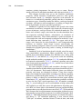
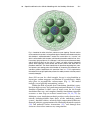
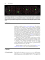
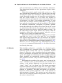
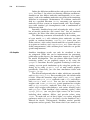
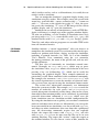
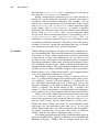
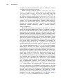
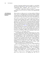
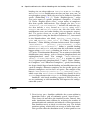
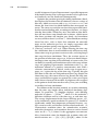
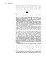
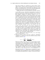
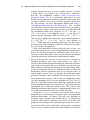
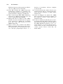
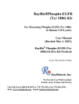
Chapter 26
Spatial and Stochastic Cellular Modeling
with the Smoldyn Simulator
Steven S. Andrews
Abstract
This chapter describes how to use Smoldyn, which is a computer program for modeling cellular systems
with spatial and stochastic detail. Smoldyn represents each molecule of interest as an individual point-like
particle. These simulated molecules diffuse, interact with surfaces (e.g., biological membranes),
and undergo chemical reactions much as they would in real biochemical systems. Smoldyn has been
used to model signal transduction within bacterial cells, pheromone signaling between yeast cells, bacterial
carboxysome function, diffusion in crowded spaces, and many other systems. A new “rule-based modeling” feature automatically generates chemical species and reactions as they arise in simulations due to
protein modifications and complexation. Smoldyn is easy to use, quantitatively accurate, and computationally efficient. It is generally best for systems with length scales between nanometers and several
microns, time scales from tens of nanoseconds to tens of minutes, and up to about 105 individual
molecules. Smoldyn runs on Macintosh, Linux, or Windows systems, is open source, and can be downloaded from http://www.smoldyn.org.
Key words: Computational biology, Smoldyn, Particle-based simulation, Spatial modeling, Rulebased modeling
1. Introduction
Computational modeling is becoming an important cell biology
research method. Modeling is useful for quantitatively testing
hypotheses about systems of interest, helping analyze and interpret experimental data, and developing a deeper understanding of
how biochemical systems function. In these and other roles, simulations have helped elucidate cellular systems such as bacterial chemotaxis (1), the eukaryotic cell cycle (2), and actin-based cellular
protrusion (3). Active simulation algorithm research and frequent
increases in computer power suggest that cellular modeling will
Jacques van Helden et al. (eds.), Bacterial Molecular Networks: Methods and Protocols, Methods in Molecular Biology,
vol. 804, DOI 10.1007/978-1-61779-361-5_26, # Springer Science+Business Media, LLC 2012
519
520
S.S. Andrews
continue gaining importance for many years to come. Recent
articles that review simulation methods and software include (4–7).
This chapter describes how to use the Smoldyn simulation
program, which simulates biochemical processes with spatial
and stochastic detail (8). Smoldyn represents each molecule of
interest as an individual point-like particle that has a location in
continuous space. Simulated molecules diffuse, undergo chemical
reactions, and interact with membranes according to simple biophysical principles and user-specified parameters.
Smoldyn is typically best for models with spatial scales from
nanometers to microns, temporal scales from tens of nanoseconds
to tens of minutes, and up to about 105 individual molecules. The
lower ends of these ranges arise from the fact that Smoldyn does
not represent excluded volumes, orientations, or momenta of
simulated molecules. These limit Smoldyn’s spatial resolution to
a few molecular radii and temporal resolution to molecules’ rotational diffusion time constants (9, 10). The upper ends of the
ranges arise from the fact that Smoldyn is too computationally
intensive to simulate much larger systems conveniently on
current desktop computers (however, recent work on parallelizing
Smoldyn for graphics processing units is starting to enable larger
simulations).
Smoldyn’s level of simulation detail is ideally suited for modeling intracellular organization. More specifically, the so-called
particle-based simulation method that Smoldyn uses (along with
ChemCell (11) and MCell (12)) has proven useful for modeling
single-molecule tracking experiments (13, 14), molecular diffusion
in restricted environments (15–17), stochastic signaling noise that
arises from spatial organization (6, 8, 18), and the causes and effects
of protein localization (19, 20).
As some examples, Lipkow and coworkers developed several
Smoldyn simulations of intracellular signal transduction for Escherichia coli chemotaxis. Each model included about ten different
proteins and about ten chemical reactions. Using these simulations, they found that intracellular crowding accentuates signaling
differences to different flagellar motors (17), that the CheZ phosphatase is likely to change its intracellular location upon cellular
stimulation (19), and that stable concentration gradients are likely
to arise for the CheY signal transducer (20). In another example
(Fig. 1), several colleagues and I used Smoldyn to help understand
why haploid yeast cells that secrete the pheromone-degrading protease Bar1 are better able to discriminate between potential mating
partners than yeast cells that do not secrete Bar1 (21). We found that
Bar1 sharpens the local pheromone concentration gradient because
pheromone is progressively inactivated as it diffuses through a Bar1
cloud (8). This model included four proteins, six chemical reactions,
and about 2 105 individual molecules; it also covered about
7,000 mm3 of volume, simulated about 75 min of time, and took
26
Spatial and Stochastic Cellular Modeling with the Smoldyn Simulator
521
Fig. 1. A model of the effect of the Bar1 protease on yeast signaling. The mesh surface
on the outside of the system is a triangulated spherical boundary that absorbs molecules
with Smoldyn’s “unbounded-emitter” method. The central sphere is a “receiver” cell
which is covered with 6,622 receptors (red if bound to pheromone and blue if not, in online version), light gray spheres are “challenger” cells which secrete pheromone slowly,
and the dark gray sphere on the right is a “target” cell which secretes pheromone
quickly. Green (light gray in print version) dots are Bar1 proteins and black dots are
pheromone molecules. This model showed that the pheromone-degrading Bar1 protease improves yeast mating partner discrimination by sharpening the pheromone concentration gradient. Republished with permission from ref. 8. The supplementary
information for the original publication presents the model parameter selection process
unusually thoroughly.
about 10 h to run. As a final example, Savage is using Smoldyn to
investigate carbon transport and fixation in cyanobacteria, which
takes place in organelle-like carboxysomes (Fig. 2). His model
includes several partially transmitting surfaces.
Within the field of particle-based simulation, Smoldyn is notable for its high accuracy and good computational efficiency (8). Each
Smoldyn algorithm is either exact or nearly exact for any length
simulation time step, and complete Smoldyn simulations approach
exactness as time steps are reduced toward zero (18, 22, 23) (by
definition, exact simulation methods produce results that are theoretically indistinguishable from those of the underlying model
system). Smoldyn achieves relatively high computational efficiency
through judicious approximations for simulating chemical reactions
(22) and molecule–surface interactions (23), and through data
structures that reduce unnecessary computations.
522
S.S. Andrews
Fig. 2. A model of carboxysome function in a cyanobacterium. The wireframe outside surface depicts the cell membrane
(internally, Smoldyn represents it as a smooth continuous surface). The four large green spheres are carboxysomes,
which are organelle-like proteinaceous compartments that contain the carbon-fixation apparatus of cyanobacteria.
Smaller red dots are carbon dioxide molecules and larger light blue dots are 3-phosphoglycerate molecules. Savage and
coworkers are using this model to investigate the roles of compartmentalization and spatial organization in carbon
fixation.
2. Materials
Smoldyn is available at http://www.smoldyn.org. The distribution includes the program source code, complete installation
instructions, a user’s manual, a programmer’s manual, example
files, and several utility programs. The Smoldyn User’s Manual is
much more thorough than this chapter and should be consulted
for statement syntax, available options, and all other details. Smoldyn is open source and runs on Macintosh, Linux, and Windows
computers (however, the Windows version does not support rulebased modeling, described in Subheading 3.10). Faster computers
run simulations faster, of course, although laptops or desktops up
to about 5 years old are often adequate.
Smoldyn runs from a shell prompt, which most operating
systems supply with a “Terminal” or “Command Prompt” application. Installation on Mac or Linux computers is typically as easy
as changing to the Smoldyn download directory and typing
./configure, make, and sudo make install at a shell
prompt. For Windows, the download includes a prebuilt Smoldyn
executable and all necessary “dll” files.
Smoldyn support is available at the on-line forum http://www.
smoldyn.org/forum, or via e-mail at [email protected].
3. Methods
3.1. Running Smoldyn
Run Smoldyn by typing smoldyn myfile.txt at a shell prompt,
where myfile.txt is your configuration file name. You can also
append option flags to this command, such as -o to suppress text
26
Spatial and Stochastic Cellular Modeling with the Smoldyn Simulator
523
output, -p to just display parameters, or -t for text-only operation. Upon starting, Smoldyn reads model parameters from your
configuration file, calculates and displays simulation parameters,
and runs the simulation. As the simulation runs, Smoldyn displays
the simulated system to a graphics window and/or saves quantitative data to one or more output files. Smoldyn stops when the
simulation is complete. Box 1 presents an example configuration
file and its output.
3.2. The Configuration
File
Smoldyn configuration files are plain text files. The first word of
each line tells Smoldyn which parameters to set and the rest of the
line lists those parameters, separated by spaces or tabs. Usually, the
statement sequence does not matter. When it does, it is usually
obvious; for example, molecular species need to be defined before
their diffusion coefficients. Smoldyn displays error messages and
terminates if it cannot parse the configuration file.
Denote comments in your configuration file with a “#”
symbol, or bracket multiple comment lines with /* and */.
Ideally, your comments should list the model name, its author or
authors, its creation and modification dates, citations to relevant
references, and the model’s distribution terms; if so, your model
will obey the “minimum information requested in the annotation
of biochemical models” (MIRIAM) (24), which aids model sharing and reuse. Your comments should also list the model units,
such as microns and seconds, or nanometers and microseconds.
This is because Smoldyn does not assume any particular units,
but instead requires that all parameters use the same units. For
example, if you choose microns and seconds, then you will need to
enter diffusion coefficients in mm2/s, first order reaction rate
constants in s1, and second order reaction rate constants in
mm3/s. See Table 3.2.1 of the Smoldyn User’s Manual.
Use read_file to separate your model description into
multiple configuration files. This can be useful for separating lists
of surface or molecule information from the main model file, or
for separating fixed model components from ones you wish to
vary. End each configuration file with end_file.
Several macro statements that substitute text “tokens” with
replacement text can simplify model development. These include
define, define_global, undefine, ifdefine, ifundefine, else, and endif. In a typical use, you would collect the
model parameters that you wish to explore to the top of your
configuration file with define statements and then refer to them
later on by their token names (see Box 1).
3.3. Space and Time
Specify whether your system is 1-, 2-, or 3-dimensional with dim.
For example, you could model protein motion along cytoskeletal
filaments in one dimension, processes on cell membranes
524
S.S. Andrews
Box 1. A sample configuration file and its output. The sections of the configuration file match those in Methods.
The snapshot was saved from Smoldyn’s graphical output at 2 seconds. The dynamics were graphed with Microsoft
Excel from data that Smoldyn saved to box1out.txt. Below, S is substrate, E is enzyme, ES is enzyme-substrate complex,
and P is product
26
Spatial and Stochastic Cellular Modeling with the Smoldyn Simulator
525
with two dimensions, or cellular systems with three dimensions.
Low-dimensional models can also approximate higher dimensional ones.
Define the system’s spatial extent with boundaries. This
does not limit the simulated space but, provided that you keep
all molecules within these boundaries, helps Smoldyn run efficiently. Internally, Smoldyn uses the boundaries to spatially partition the system volume so as to reduce the number of
molecule–molecule and molecule–surface interactions that it has
to investigate (see Note 1 for partition optimization). If your
model does not include surfaces (Subheading 3.7), then specify
how molecules should interact with the boundaries. The options
are reflection, transmission, absorption, or periodic (periodic
means that molecules that diffuse out of one side of the system
are immediately diffused into the opposite side of the system,
which can avoid edge effects in effectively infinite systems). On
the other hand, if your model includes any surfaces, then the
boundaries defined here will only transmit molecules and you
will have to use surfaces to confine molecules.
Specify the simulation starting time, stopping time, and time
step with time_start, time_stop, and time_step. Smoldyn
only supports fixed-length time steps, in contrast to the adaptive
time steps that MCell supports (12) or the event-based time steps
that the Green’s Function Reaction Dynamics method uses (25).
However, you can change time steps midsimulation with the
settimestep command (Subheading 3.6). See Note 2 for advice
on choosing time steps.
3.4. Molecules
Each Smoldyn molecule is a member of a chemical species,
and all molecules of a particular species are equivalent. Enter
individual species names with species statements. Distinct
forms of a molecule, such as phosphorylated and unphosphorylated, or monomeric and dimeric, need to be defined as separate
species. To simplify the definitions for these multiple molecular
forms, Smoldyn can automatically enumerate both them and
their chemical reactions using rule-based modeling (Subheading 3.10).
Each molecule, regardless of its species, may be in any of five
states. “Solution” state, in which molecules are not bound to
surfaces, is the default. Molecules can also bind surfaces in a
“front,” “back,” “up,” or “down” state. The former two options
represent molecules that bind a single side of a surface, where
typical uses include peripheral membrane proteins, GPI-anchored
proteins, or adsorbates. The other two options, up and down,
represent surface-spanning molecules, such as ion channels or
trans-membrane receptors. The separate up and down states
allow one to distinguish whether the protein’s active side faces
the surface’s front or back.
526
S.S. Andrews
Define the diffusion coefficient for each species and state with
See Note 3 for advice on choosing diffusion coefficients.
Smoldyn can also diffuse molecules anisotropically (difm statement), such as for confining molecules to a plane or for simulating
diffusion in anisotropic environments. In addition, molecular
drift in a specified direction (drift statement) can represent
molecules in flow systems or around motile cells. For example,
you could simulate gel electrophoresis with a combination of
diffusion and drift.
Internally, Smoldyn keeps track of molecules with a “dead”
list of inactive molecules and several “live” lists of simulated
molecules. See Note 4 for advice on arranging the live lists.
The following statements add molecules to the starting state
of your model: mol adds solution phase molecules to either
specific or random locations; surface_mol (enter after you
define surfaces) adds surface-bound molecules to specific surfaces
or regions on surfaces; and compartment_mol (enter after you
define compartments) adds solution phase molecules to specific
spatial compartments.
difc.
3.5. Graphics
Smoldyn simulation results can only be visualized as they
are computed. While this can be inconvenient for generating
publication quality figures, the immediate output is very helpful
for model development. You can choose from three levels of
rendering quality, or no graphical output at all, using the
graphics statement. Because graphical rendering is time-consuming, you can speed simulations up by using low quality rendering or by using graphic_iter to only render graphics
periodically. Conversely, you can slow simulations down with
graphic_delay.
The default background color is white, which you can modify
with background_color. For everything else, the default color
is black. Color the boundary edges with frame_color, spatial
partitions with grid_color, molecules with color, and surfaces
with surface name color. You can also set boundary line
weights with frame_thickness, spatial partition line weights
with grid_thickness, molecule sizes with display_size,
surface edge weights with thickness, and surface drawing styles
with polygon. With Smoldyn’s best rendering quality, called
opengl_better, you can place light sources in the system,
including their ambient, diffuse, and specular colors, using
light. To make full use of these lights, set surface reflection
parameters with shininess. As always, see the Smoldyn User’s
Manual for details. Unfortunately, Smoldyn renders partially
transparent surfaces poorly. This means that if you want to see
26
Spatial and Stochastic Cellular Modeling with the Smoldyn Simulator
527
what’s inside a surface, such as a cell membrane, it is usually best to
render it with a wireframe.
You can manipulate Smoldyn’s graphical display during your
simulation using key strokes. For example, rotate the system with
arrow keys, pan with shift + arrows, zoom in with “¼,” zoom out
with “,” or revert to the default view with “0.” Also, the space
bar pauses the simulation, “T” saves a TIFF image of the current
graphics display, and “Q” quits the simulation.
Smoldyn can save movies of simulations as stacks of TIFF files.
Again, each image is a simple copy of the graphics window display.
To turn on recording, set the number of simulation time steps
per image with tiff_iter, name the files with tiff_name, and
number the files with tiff_min and tiff_max. ImageJ, QuickTime Pro, and other software programs can assemble TIFF stacks
into self-contained movies.
3.6. Runtime
Commands
Smoldyn includes a “virtual experimenter” who can observe or
manipulate the simulated system. You can instruct this virtual experimenter to perform tasks before, during, or after the simulation,
including at periodic intervals (see Table 3.6.1 of the Smoldyn
User’s Manual). Issue commands using the cmd statement,
the timing parameters, the name of the specific task, and any taskspecific parameters.
The first class of commands are simulation control commands. Examples are stop and pause, which stop or pause
the simulation. Also, keypress mimics the behavior of the user
pressing a key (see Subheading 3.5), which can be useful for
automating the graphical display. These control commands are
particularly useful when combined with conditional commands.
For example, the statement “cmd E ifno substrate stop” tells
the virtual experimenter to count the number of substrate molecules at every time step and to stop the simulation if none remain.
The second class, observation commands, save information
about the system to text files. For example, molcount records the
number of molecules for each species and molcountspace
records histograms of molecule counts along a line in the system,
from which concentration profiles can be calculated. A particularly
powerful observation command is savesim, which saves the
entire simulation state to a Smoldyn-readable configuration file.
By saving the simulation state regularly, you can abort a simulation
mid-run and then restart it later on. Alternatively, you can equilibrate your model in one simulation, save the result with savesim,
and then run other simulations that start from this equilibrated
state. All observation commands require that you explicitly
declare the output file names with output_files, and also
with output_root if you do not want the files to be in your
working directory. The output file “stdout” sends the output to
the terminal window. To save data to a series of files, number the
528
S.S. Andrews
first one with output_file_number and progress to subsequent
ones with the incrementfile command.
Finally, manipulation commands give you wide latitude to
modify the system during the simulation, and not necessarily in
accordance with biochemical principles. For example, you can
instruct the virtual experimenter to add molecules to the system
with pointsource or volumesource, remove molecules from
inside spheres with killmolinsphere, or replace a specified
fraction of one molecular species in some volume with a different
species using replacevolmol. Also, several commands allow
you to create fixed concentration inputs to your model, such as
fixmolcountonsurf and fixmolcountincmpt. The set
command is extremely powerful because you can follow it with
essentially any Smoldyn statement. This allows you to add species,
reactions, or surfaces, change the simulation time step, or modify
your model in many other ways, all mid-simulation.
3.7. Surfaces
Unlike biological membranes or other real surfaces, Smoldyn surfaces are infinitely thin. This means that molecules in solution phase,
or in “front” or “back” surface-bound states, are always on the front
or back side of a surface; also, molecules in “up” or “down” states
are always exactly at the surface. Each Smoldyn surface is composed
of geometric primitives called panels, which can be triangular, spherical, cylindrical, or other shapes. Along with being convenient and
computationally efficient, this representation method is also quite
versatile because it allows arbitrarily complex surface geometries,
disjoint surfaces (e.g., a collection of vesicles), and/or open surfaces
(e.g., the fragmented membrane of a lysed cell).
For example, the model shown in Fig. 1 includes four surfaces: (1) a mesh of 480 triangles that surrounds the entire system,
(2) a spherical “receiver” cell in the middle, (3) a spherical “target” cell shown toward the right side in dark gray, and (4) five
spherical “challenger” cells shown in light gray. Note that this last
surface is disjoint. The model shown in Fig. 2 includes two
surfaces: (1) the cell membrane, assembled from two hemispheres
and a cylinder and (2) four spherical carboxysome protein shells.
Define each surface with a block of statements that starts with
start-surface and ends with end_surface (you can also
enter surface parameters with statements that start with surface
and the surface name, but the block format is usually easier).
Within this block, Within this block, list each individual panel
with panel. list each individual panel with panel. If you want
surface-bound molecules to be able to diffuse between neighboring panels, whether they are on the same surface or different
surfaces, then list each panel’s neighbors with neighbor.
Two utility programs included in the distribution help generate
panel and neighbor data. The first, wrl2smol, reads Virtual Reality
Modeling Language (VRML) files of triangle mesh data and
26
Spatial and Stochastic Cellular Modeling with the Smoldyn Simulator
529
converts them to lists of triangle panels and their neighbors in
Smoldyn format. Mathematica, MatLab, ImageJ, and other programs can generate VRML files. The second utility program,
SmolCrowd, generates random arrays of nonoverlapping circles or
spheres, which can be useful for modeling macromolecular
crowding.
Several parameters characterize each surface. These include
graphical display parameters, described in Subheading 3.5, and
surface–molecule interaction parameters. Many types of interactions are possible. For example, you can make a surface impermeable, transmitting, or irreversibly absorbing for molecules that
diffuse into it, and these interactions can differ for different
molecular species and the two surface faces. Specify these behaviors with action. Alternatively, specify coefficients for adsorption to, desorption from, or partial transmission through surfaces
(23) with rate (see Note 5 for advice on these coefficients). Two
molecular pseudo-states, “fsoln” and “bsoln,” allow you to
distinguish solution-state molecules on the front side of a surface
from solution-state molecules on the back side of a surface. You
can also specify rates for transitions between surface-bound states,
such as from the front state to the back state. Additionally, you can
instruct molecules to change species when they cross a surface;
this is particularly useful for models with spatially variable diffusion coefficients, such as between extracellular and intracellular
regions, or nonraft and raft regions of membranes. Jump surfaces
(defined with action and jump) magically transport molecules
from one panel to another. They are useful for adding
holes to otherwise impermeable surfaces, such as pores in a
nuclear envelope, and for creating periodic boundaries. Finally,
unbounded-emitter surfaces (unbounded_emitter statement)
irreversibly absorb molecules with coefficients that make internal
concentration profiles mimic those that would be seen for
an unbounded system (23). The triangulated mesh in Fig. 1 is
an unbounded-emitter surface.
3.8. Chemical
Reactions
Smoldyn supports zeroth, first, and second order chemical reactions, where the order is just the number of reactants. Use zeroth
order reactions to add molecules at random locations within the
entire system volume or within a compartment (Subheading 3.9)
at a roughly constant rate. These violate mass balance and are thus
unphysical; however, they are particularly useful for including
protein or mRNA synthesis in models but not the respective
synthesis machinery. Use first order, or unimolecular, reactions
for spontaneous molecular changes, such as protein conformation, dissociation, and decay processes. These are also useful for
pseudo-first order reactions, in which one of two reactants
(e.g., ATP) is unmodeled and assumed to be constant and
uniformly distributed. Use second order, or bimolecular,
530
S.S. Andrews
reactions for interactions between pairs of molecules, such as
association and enzymatic reactions.
Enter reactions with the syntax: “reaction name reactants —> products rate,” where name is the reaction name,
reactants and products are lists of species and states that
are separated by “+” symbols (use “0” if a list is empty and use
the fsoln and bsoln pseudo-states as necessary), and rate is the
reaction rate constant. Alternatively, use reaction_surface or
reaction_cmpt for reactions that should only occur on specific
surfaces or in specific compartments. Smoldyn allows up to 16
products for each reaction. Note 6 offers advice on choosing
reaction rate constants and Note 7 describes ways to speed up
bimolecular reaction simulation, which is typically Smoldyn’s
slowest component.
Reversible association reactions, of the form A + B ↔ C,
involve an additional complication. When a C molecule dissociates,
the new A and B molecules form in close proximity to each other,
which makes them especially likely to react with each other. This
reaction between dissociation products is called a geminate recombination. Nonspatial treatments of chemical kinetics, including conventional mass-action theory and nonspatial simulations, cannot
account for geminate recombinations, so they are often ignored.
However, geminate recombinations affect reaction rates both in
real systems and in particle-based simulations. For example, the
association reaction rate for A + B ↔ C is faster if it is measured at
equilibrium than if it is measured with all C removed as it is formed
(e.g., with the additional reaction C + D ! E, and a high concentration of D), because the former situation includes geminate
recombinations and the latter does not. So that Smoldyn can accurately simulate the kinetics of reversible reactions, and other reactions where the products can react with each other, you need to
specify how Smoldyn should place dissociation products in the
system with product_placement. Ideally, you should choose
the placement method that represents whether the experimental
rate constants were measured at equilibrium or with products
removed as they were formed (see Table 3.8.2 of the Smoldyn
User’s Manual); and you should also give the probability of geminate recombinations. However, these details are almost never
known, so I suggest using “product_placement name pgemmax
0.2,” where name is the reaction name. This states that reaction
rates were measured at equilibrium (typically correct) and that
reaction products should have up to a 20% probability of recombining with each other. This geminate recombination probability
typically leads to efficient simulations and physically sensible
simulation parameters (the binding and unbinding radii (18, 22)).
Smoldyn uses the same parameters if you do not enter a
product_placement statement, but issues a warning.
26
Spatial and Stochastic Cellular Modeling with the Smoldyn Simulator
531
Smoldyn also uses the bimolecular reaction formalism for conformational spread and excluded volume interactions. Use conformational spread interactions to model mechanical coupling between
stationary molecules (set the maximum interaction distance with
confspread_radius). The prototypical conformational spread
example occurs in the E. coli flagellar motor, in which motor proteins in “active” conformations induce activity in their neighbors
and those with “inactive” conformations induce inactivity in their
neighbors (26); this positive feedback makes the motor switch-like.
Excluded volume interactions (product_placement statement)
keep molecules spatially separate. They are particularly useful for
keeping molecules that are confined to a channel from passing each
other. They also permit more general simulations of molecules with
excluded volume, although this aspect of Smoldyn is computationally inefficient.
3.9. Spatial
Compartments
Smoldyn compartments are regions of volume bounded by surfaces.
A cell’s cytoplasm, nucleus, or extracellular space are typical examples. Compartments are useful for specifying initial conditions of
models, for recording simulation results, for defining reactions that
are only relevant in specific regions, and for compatibility with
compartment-based simulators (e.g., Virtual Cell (27) and
MOOSE (28)). To use compartments, define individual compartments with blocks of statements bracketed by start_compartment and end_compartment.
You can define a compartment with either of two methods, or
with a combination of them. In the first, list the compartment’s
bounding surfaces (the same surfaces that Subheading 3.7
describes) with surface statements and list one or more
“inside-defining” points with point statements. These points
define the compartment’s volume as follows: a molecule is defined
to be in a compartment if and only if a straight line can be drawn
between it and an inside-defining point without crossing one of
the compartment’s bounding surfaces. For example, we could
define a compartment for the model shown in Fig. 2 that included
the entire bacterial volume, which we’ll call “cell,” by making the
cell membrane the compartment surface and listing an interiordefining point near the center of the cell. This compartment
would behave as one would expect, where any molecule within
the bacterium (including molecules in carboxysomes) would be in
the “cell” compartment and any molecule outside of the bacterial
membrane would not be in the “cell” compartment. We could
define another compartment that included all of the carboxysome
interiors, called “carboxysome,” by setting the compartment
surface to the carboxysome surface (which is disjoint) and listing
an interior-defining point at the center of each carboxysome.
The other way to define a compartment is with logical combinations of previously defined compartments, using the compartment
532
S.S. Andrews
statement. Continuing with the previous examples, we could define
the bacterial cytoplasm in Fig. 2 that is not within a carboxysome as a
compartment called “cytoplasm” with “compartment equal
cell” and then “compartment andnot carboxysome.”
Overall, this compartment definition method is somewhat
nonintuitive, but it is easy to use, versatile, and computationally
efficient.
3.10. Rule-Based
Reaction Network
Expansion
Most proteins can adopt any of a very large number of different
states, such as by phosphorylation, nucleotide-binding, multiple
conformations, or complexation with other proteins. In Smoldyn,
as in most simulators, each of these states needs to be modeled as a
distinct species, with distinct chemical reactions. Manually listing
these species and their reactions is often impractical though, so
modelers typically simplify their models to only include the most
essential states, while ignoring the rest. The drawbacks of this
approach are, of course, that it can overlook important biological
interactions and it precludes the study of realistic reaction networks.
Thus, several groups have pursued a different approach, in which the
simulator generates the species and chemical reactions automatically
from “interaction rules” (29, 30). Smoldyn supports this so-called
rule-based modeling with a module called libmoleculizer. A notable
libmoleculizer feature is that it only generates species and their
reactions as they arise; this means that Smoldyn does not need to
keep track of multimeric complexes that could theoretically exist,
but that never actually form. This speeds simulations, reduces computer memory use, and simplifies models.
In the libmoleculizer formalism, chemical species are assembled from building blocks called mols. Both individual mols and
multimeric complexes of mols are chemical species. Each mol can
have modification sites, such as for phosphorylation, methylation,
or nucleotide-binding. Also, each mol can have binding sites
with which it can reversibly bind other mols to form multimeric
complexes. These binding sites have “shapes” so that their activity
can be modulated through allosteric interactions. For example, a
binding site can be put in its “active” shape when a specific
modification site is phosphorylated, and in its “inactive” shape
when that modification site is unphosphorylated.
Enter network generation rules in your configuration file in
a block of statements that starts with start_rules and ends
with end_rules. Within this block, enter rules in the following
categories. (1) Under “Modifications,” declare all possible posttranslational modifications. For example, “name ¼ PP” might represent double phosphorylation. (2) Under “Molecules,” define
the mols, their binding sites, and their modification sites. For
example, “Fus3(ToSte5, ToSte12 {inactive, active},
*PhosSite {None,P,PP})” states that Fus3 is the name of a
mol, ToSte5 and ToSte12 are binding sites, the ToSte12
26
Spatial and Stochastic Cellular Modeling with the Smoldyn Simulator
533
binding site can adopt either an inactive or an active shape,
and PhosSite is a modification site that can have zero, one, or
two phosphate groups. Mols also need to be defined as Smoldyn
species (Subheading 3.2). (3) Under “Explicit-Species,” assign
your own names to specific multimeric complexes, if desired.
(4) Under “Explicit-Species-Class,” assign names to complexes
that share specific characteristics. For example, the class “Fus3
(ToSte12!1).Ste12(ToFus3!1)” includes all molecular species that include a Fus3 bound to a Ste12, using Fus3’s
ToSte12 site and Ste12’s ToFus3 site; this class leaves other
modification states and other binding site occupancies unspecified. Use species classes to set the graphical display of newly
generated species using the Smoldyn statements (i.e., not entered
in the libmoleculizer rule block) species_class_display_
size and species_class_color. (5) Under “AssociationReactions,” define binding reactions between mols. For example,
“Fus3(ToSte12
{active}) + Ste12(ToFus3) —> Fus3
(ToSte12!1).Ste12(ToFus3!1)” defines a possible binding
between Fus3 and Ste12, and states that this association can only
happen when Fus3’s ToSte12 binding site is in its active shape.
(6) Under “Transformation-Reactions,” list reactions in which mol
modification states change, such as between phosphorylated and
unphosphorylated states. For example, “Fus3(*PhosSite
{None}) —> Fus3(*PhosSite {P})” is a reaction in which
Fus3 is spontaneously phosphorylated. (7 and 8) Under “Allosteric-Complexes” and “Allosteric-Omniplexes,” specify how binding
site shapes should depend on the binding and modification states of
a mol or complex. Allosteric-complexes are for specific species and
allosteric-omniplexes are for classes of species. An example of the
latter is “Fus3(ToSte12 {active <— *}, *PhosSite {PP})”
which states that Fus3’s ToSte12 binding site should be in its
active shape whenever the PhosSite is doubly phosphorylated.
Smoldyn’s rule-based modeling support is still very new, so
we are continuing to add functionality and improve the configuration file syntax.
4. Notes
1. Partitioning space. Smoldyn subdivides the system within its
boundaries into a grid of uniformly spaced “virtual boxes.”
These boxes do not affect the simulated results. Instead, they
make simulations more efficient by reducing the number of
potential molecule–molecule and molecule–surface interactions
that Smoldyn needs to check at each time step. The default
partition spacing, which yields an average of about four molecules per box when the simulation starts, is often good but can
534
S.S. Andrews
usually be improved upon. Improvement is especially important
if the model starting state is not representative of its typical state
or if molecules are not distributed homogenously.
Optimize the partition spacing by timing simulations (Smoldyn displays the run time when it terminates) that use a range of
box sizes, which you can set with molperbox or boxsize, and
choose the fastest size for which Smoldyn does not report any
errors. The errors to watch for are those that report that bimolecular reaction binding radii, or analogous distances, are larger
than the box widths. When they arise, they indicate that Smoldyn will not detect some bimolecular reactions, which means
that those reactions will simulate too slowly, and simulation
accuracy will be reduced (see Note 7). Other Smoldyn warnings
about box sizes, such as those that comment on unusually
many or few molecules per box, are simply suggestions that
different partition spacings may improve performance.
2. Choosing simulation time steps. When choosing the time step
for a simulation, there is an unavoidable trade-off between using
shorter time steps to get more accurate results, and using longer
time steps for faster simulations. Thus, the succinct answer to
the question of what time step to use, is that you should choose
the longest time step that yields sufficiently accurate results. You
can find it by running trial simulations with a wide range of time
steps and graphing representative simulation results (e.g., the
maximum amount of a product concentration, time until a
substrate concentration is halved, steady-state receptor occupancy, etc.) against the log of the time step. Typically, this plot
will show results that are independent of time step lengths for
short time steps, that errors increase log-linearly for long time
steps, and that these regions are separated by a cross-over region
that is about a factor of 10 in width. A judgment call is required
at this point to decide how much accuracy, if any, you are willing
to sacrifice for faster simulations.
In addition to this heuristic method, it is worth considering
how the time step length affects individual simulation algorithms. In particular, (1) Smoldyn displaces each diffusing
molecule by about s ¼ (2DDt)1/2, where D is the molecule’s
diffusion coefficient and Dt is the time step, at each time step.
The average displacement for the fastest diffusing species, smax,
is the simulation’s spatial resolution. In general, smax should be
significantly smaller than important geometrical features, surface curvature radii, and distances between fixed molecules. (2)
Characteristic transition times for unimolecular reactions,
molecular desorption, and transitions between surface-bound
states are all t ¼ 1/k, where k is the appropriate rate constant.
Also, characteristic times for bimolecular reactions with wellmixed reactants are t ¼ ([A] + [B])/(k[A][B]), where k is the
26
Spatial and Stochastic Cellular Modeling with the Smoldyn Simulator
535
reaction rate constant and [A] and [B] are the reactant
concentrations. And, characteristic times for molecular adsorption and permeability are t ¼ d/k, where d is the distance
between surfaces (e.g., the cell length) and k is the adsorption
or transmission coefficient. To simulate these dynamics accurately, the time step should be smaller than these characteristic
times. (3) Smoldyn performs bimolecular reactions between
pairs of reactant molecules that are closer than their “binding
radius.” Binding radii, which Smoldyn computes from reaction
rates, diffusion coefficients, and the simulation time step,
increase as time steps are made longer and are often larger
than physical molecular radii (22). If a molecular species is so
concentrated that these binding radii frequently overlap each
other, which is especially problematic for clustered surfacebound molecules (e.g., the receptors in Fig. 1 (8)), this
decreases accuracy. (4) For fast bimolecular reactions that are
far from steady state, Smoldyn’s simulated results more closely
agree with diffusion-limited kinetics when short time steps are
used and with activation-limited kinetics when long time steps
are used (22). This is unlikely to affect typical biochemical
network models, but may affect reaction biophysics models.
For all of these time step considerations, note that Smoldyn
displays all internal simulation parameters, several characteristic
times, and any warnings for potential problems before it starts
simulations. It is prudent to check that this information seems
reasonable.
In practice, many researchers use time steps around 0.1 ms
(16, 17, 19, 20, 31, 32). Smoldyn has also been used with time
steps as short as 0.06 ns, in a test of its reaction algorithms
(22), and with time steps up to 10 or 20 ms (8, 33). The latter
models, one of which is shown in Fig. 1, were able to use long
time steps because they had relatively low molecular densities
and large system geometries.
3. Choosing diffusion coefficients. In homogeneous solutions, such
as water or liquid growth media, diffusion coefficients can often
be approximated reasonably well with the Stokes–Einstein equation. It is
D¼
kB T
;
6pr
where D is the diffusion coefficient, kB is Boltzmann’s constant,
T is the absolute temperature, is the solution viscosity, and r is
the radius of the diffusing particle, which is assumed to be
spherical. This particle radius can be easily calculated from its
mass m and density r,
sffiffiffiffiffiffiffiffi
pffiffiffiffiffi
3 3m
r¼
0:0655 3 m nm:
4pr
536
S.S. Andrews
In the latter equality, m is measured in Daltons; also, it assumes
an average density of 1.41 g/cm, which is reasonably accurate
for proteins above 40 kDa and within 10% for smaller proteins
(34). Combining this radius calculation with the Stokes–
Einstein equation yields the protein diffusion coefficient estimate
3270
ffiffiffiffiffi mm2 /s:
D p
3
m
This is for a temperature of 20 C, where water’s viscosity is very
nearly 1 mPa s. Two examples are: for lysozyme, m is 14.6 kDa,
the experimental D is 111 mm2/s (35), and the computed D is
134 mm2/s; and for green fluorescent protein (GFP), m is
26.9 kDa, the experimental D is 87 mm2/s (36, 37), and the
computed D is 109 mm2/s. Of course, theories that account for
protein shape yield better predictions (35).
For small molecules in water, experimentally measured diffusion coefficients are readily available. Examples include
2,010 mm2/s for oxygen at 20 C and 380 mm2/s for lactose at
15 C (38). For quick estimates, the Stokes–Einstein equation is
usually correct to within a factor of two.
In eukaryotic cytoplasms, nuclei, and mitochondria, experiments by Verkman’s group show that macromolecule diffusion
coefficients are about 25% of their values in water, for masses
up to about 500 kDa (39, 40). Larger molecules and filamentous molecules, such as DNA, diffuse more slowly, likely due to
sieving by actin networks. In the E. coli bacterial cytoplasm,
GFP diffuses about another factor of 5 slower than it does
in eukaryotes, now with a diffusion coefficient around
3–8 mm2/s (41, 42). Diffusion is much slower yet in the
E. coli periplasm, where the 42.5 kDa maltose-binding protein
has a diffusion coefficient of about 0.009 mm2/s (43). Finally, a
couple of membrane-bound protein diffusion coefficients are
0.09 mm2/s for aquaporin-1 (about 30 kDa) in nonpolarized
fibroblast cell membranes (44) and 0.012 mm2/s for histidine
kinase PleC (117 kDa, including fluorophore) in Caulobacter
membranes (14).
From these data, I suggest the rules-of-thumb: use 80% of
the Stokes–Einstein value, as calculated above, for proteins in
water, and divide the aqueous diffusion coefficient by 4 for
eukaryotic cell and organelle cytoplasms, by 15 for bacterial
cytoplasms, by 1,000 for bacterial periplasms, by 1,000 for
eukaryotic membranes, and by 4,000 for bacterial membranes.
4. Optimizing molecule lists. As Subheading 3.4 mentions, Smoldyn stores molecules in several lists. By default, Smoldyn stores
all simulated molecules that do not diffuse in a “fixed” list and
26
Spatial and Stochastic Cellular Modeling with the Smoldyn Simulator
537
those that do diffuse in a “diffusing” list. This scheme is more
efficient than a single list because Smoldyn does not need to
diffuse or perform surface interactions for molecules in the
fixed list; also Smoldyn does not need to check for bimolecular
reactions between pairs of molecules in the fixed list.
Adding more lists can speed simulations up further, often by
factors of five or more, typically by minimizing the number of
potential bimolecular reactions that Smoldyn needs to check.
For example, consider the chemical reaction A + B ! C.
If Smoldyn stored all three species in the same list, then when
Smoldyn searched the list to see which AB molecule pairs could
react, it would also encounter many nonreactive AA, AC, BB,
BC, and CC molecule pairs, each of which would take a small
amount of time to check and then ignore. On the other hand,
Smoldyn would only encounter AB pairs if A, B, and C were
stored in three separate lists. Generalizing this example, more
molecule lists reduce the number of unnecessary checks, so
typically produce faster simulations. This trend does not continue indefinitely though, because each molecule list also
requires some processing time; this becomes important for
lists with few molecules. Thus, overall, simulation performance
is usually best when each abundant species has its own list
and when sparsely populated species share lists. Further list
optimization, by considering the potential bimolecular and
molecule–surface interactions that Smoldyn has to check at
each time step, can produce additional gains.
Create molecule lists with molecule_lists and assign
species to them with mol_list.
5. Choosing molecule–surface interaction coefficients. Adsorption
coefficients are limited to about the thermal velocity of the
adsorbent, which is (45)
rffiffiffiffiffiffiffiffiffi
kB T 1:56 109
pffiffiffiffiffi
kmax ¼
mm/s:
m
m
The latter equality assumes that m is measured in Daltons and the
temperature is 20 C. For example, the largest possible adsorption coefficient for a 50 kDa protein is about 7 106 mm/s. Real
adsorption coefficients are likely to be vastly smaller than this
maximum. For example, Huang and coworkers chose an adsorption coefficient of 0.025 mm/s for the adsorption of MinD
(29.5 kDa) to the inside of the E. coli cell membrane in a
biochemical model (46). Unfortunately, remarkably few experimental papers present quantitative data on protein adsorption to
or desorption from lipid bilayers, despite an extensive literature.
538
S.S. Andrews
Transmission coefficients for molecules through membranes
can be calculated using the equation (47)
k¼
Kmem Dmem
;
dmem
where Kmem is the partition coefficient for the molecule into the
membrane from the neighboring solution (e.g., cytoplasm),
Dmem is the molecule’s diffusion coefficient in the membrane,
and dmem is the membrane thickness. Qualitatively, this equation
shows that hydrophobic molecules are transmitted faster than
hydrophilic ones because they partition into the membrane
more readily, and that smaller molecules are transmitted faster
than larger ones because they diffuse faster. A paper by Paula
et al. (47) shows how to compute the necessary parameters. It
also lists some experimentally determined coefficients for transmission through lipid bilayers, including: 3.5 108 mm/s for
potassium ions, 0.014 mm/s for urea, 0.027 mm/s for glycerol,
5 mm/s for protons, and 150 mm/s for water molecules; these
values are for 2.7 nm thick bilayers, which is about the thickness
of typical biological membranes.
Adsorption and transmission coefficients can also be estimated using the respective characteristic times (see Note 2), if
these times can be inferred from experiments.
6. Choosing reaction rate constants. Experimental bimolecular
reaction rates are limited to
kmax ¼ 4pðDA þ DB ÞðrAs þ rB Þ
by the rate at which reactants can diffuse together (48). Here,
kmax is the diffusion-limited reaction rate constant, DA and DB
are the diffusion coefficients of the reactants, and rA and rB are
the reactant radii. Highly reactive small molecules sometimes
react with rates that are close to this maximum (49), but typical
biochemical reaction rate constants are much slower. You can
verify that your simulated rates will be well below this maximum by comparing Smoldyn’s output parameter labeled
“binding radius if dt were 0” to the sum of the physical reactant
radii. They will be equal if your simulated reaction is at the
maximum rate, and proportionately less for slower reactions.
Other than this one qualitative check, reaction rates usually
have to found from the scientific literature that is relevant to your
model. Typically, some reaction rates will have been measured,
others can be calculated from published data (e.g., association
reaction rates can be calculated from dissociation constants
and dissociation reaction rates), others can be estimated from
characteristic reaction times and published figures, and yet
others simply have to be guessed. Previously developed
26
Spatial and Stochastic Cellular Modeling with the Smoldyn Simulator
539
models, whether of your system or similar systems, are often
a good source of reaction rates and literature references.
For this, the BioModels database (http://www.ebi.ac.uk/
biomodels-main) (50) is a particularly good place to start.
Finally, curated literature summaries that list quantitative data
are rarely available, but can be excellent resources when they
are. For example, the Yeast Pheromone Model wiki (http://
yeastpheromonemodel.org/wiki/Main_page) lists reaction
rates and their references for most reactions in the yeast pheromone response system. A few representative rates from this wiki
are pheromone binds Ste2 receptors at 1.8 105 M1 s1
(3.1 104 mm3/s) and unbinds at 103 s1, the Gpa1 Gprotein subunit exchanges GDP for GTP at 6.17 104 s1,
and the Fus3 MAP kinase binds the Ste5 scaffold protein at
2.3 106 M1 s1 (3.8 103 mm3/s) and unbinds at
2.3 s1. While these are reasonably typical values for these types
of interactions, other similar reactions are often faster or slower
by several orders of magnitude.
Note that bimolecular reactions that take place in one- and
two-dimensional systems, such as along filaments or within membranes, do not have reaction rate constants in the same sense as
reactions in three dimensions. Also, current versions of Smoldyn
cannot quantitatively simulate low-dimensional reactions.
7. Lowering bimolecular reaction accuracy for faster simulations.
Smoldyn partitions space into virtual boxes (see Note 1)
to reduce the number of potential molecule–molecule and molecule–surface interactions that need checking at each time step.
Most molecule–molecule interactions occur within single boxes
in typical simulations. However, Smoldyn also has to check for
interactions between molecules that are in adjacent boxes to
achieve high accuracy. There are typically about 50 times more
potential “interbox” than “intrabox” interactions because (1) in
three-dimensional systems, each box has 26 neighboring boxes
(or eight neighbors in 2-D or two neighbors in 1-D), and (2)
there are n2 possible pairwise interactions for n molecules in each
of two neighboring boxes but only about n2/2 possible pairwise
interactions for n molecules within a box. The result is that
checking for interbox interactions is computationally costly, relative to the few interactions that are actually detected.
Using the accuracy statement, you may be able to speed
Smoldyn up by instructing it to ignore some or all potential
interbox interactions. Of course, this will cause Smoldyn to
overlook some reactions that should occur, so bimolecular
reactions will simulate somewhat too slowly. If desired, this
problem can be mitigated by determining reaction rate correction factors from trial simulations (alternatively, correction
factors can be estimated from the total numbers of intrabox
540
S.S. Andrews
and interbox reactions, which Smoldyn reports upon termination). In practice, the simulation speed improvement is typically much less than the maximum possible factor of 50, and is
often just a factor of 2 or less. Thus, the best approach is to try
lowering Smoldyn’s accuracy parameter and directly assessing
how much the simulation speed improved and how much the
actual accuracy decreased.
Acknowledgments
I thank Nathan Addy for developing the Smoldyn build system and
the libmoleculizer module, David Savage for providing the configuration file for Fig. 2, and Roger Brent for encouragement and
helpful discussions. I also appreciate helpful comments and suggestions from many Smoldyn users, including Karen Lipkow and
Shahid Khan in particular. This work was supported by MITRE
contract number 79729, awarded to Roger Brent.
References
1. Tindall MJ, Porter SL, Maini PK, Gaglia G,
Armitage JP. (2008) Overview of mathematical approaches used to model bacterial chemotaxis I: the single cell. Bull Math Biol,
70:1525–1569.
2. Tyson JJ, Novak B. (2008) Temporal organization of the cell cycle. Curr Biol, 18:
R759–R768.
3. Mogilner A. (2006) On the edge: modeling
protrusion. Curr Opin Cell Biol, 18:32–39.
4. Alves R, Antunes F, Salvador A. (2006) Tools
for kinetic modeling of biochemical networks.
Nat Biotechnol, 24:667–672.
5. Takahashi K, Arjunan SNV, Tomita M. (2005)
Space in systems biology of signaling pathways
– towards intracellular molecular crowding in
silico. FEBS Lett, 579:1783–1788.
6. Andrews SS, Arkin AP. (2006) Simulating cell
biology. Curr Biol, 16:R523–R527.
7. Andrews SS, Dinh T, Arkin AP. (2009)
Stochastic Models of Biological Processes.
In Encyclopedia of Complexity and System Science. Vol. 9. Edited by Meyers RA, Springer,
New York, 8730–8749.
8. Andrews SS, Addy NJ, Brent R, Arkin AP.
(2010) Detailed simulation of cell biology
with Smoldyn 2.1. PLoS Comp Biol, 6:
e1000705.
9. Dayel MJ, Hom EFY, Verkman AS. (1999)
Diffusion of green fluorescent protein in the
aqueous-phase lumen of endoplasmic reticulum. Biophys J, 76:2843–2851.
10. Partikian A, Ölveczky B, Swaminathan R, Li Y,
Verkman AS. (1998) Rapid diffusion of green
fluorescent protein in the mitochondrial
matrix. J Cell Biol, 140:821–829.
11. Plimpton SJ, Slepoy A. (2005) Microbial cell
modeling via reacting diffusive particles.
J Phys Conf Ser, 16:305–309.
12. Kerr RA, Bartol TM, Kaminsky B, Dittrich M,
Chang J-CJ, Baden SB, Sejnowski TJ, Stiles
JR. (2008) Fast Monte Carlo simulation
methods for biological reaction-diffusion systems in solution and on surfaces. SIAM J Sci
Comput, 30:3126–3149.
13. Jin S, Haggie PM, Verkman AS. (2007)
Single-particle tracking of membrane protein
diffusion in a potential: simulation, detection,
and application to confined diffusion of CFTR
Cl channels. Biophys J, 93:1079–1088.
14. Deich J, Judd EM, McAdams HH, Moerner
WE. (2004) Visualization of the movement of
single histidine kinase molecules in live Caulobacter cells. Proc Natl Acad Sci U S A,
101:15921–15926.
15. Coggan JS, Bartol TM, Esquenazi E, Stiles JR,
Lamont S, Martone ME, Berg DK, Ellisman
MH, Sejnowski TJ. (2005) Evidence for
ectopic neurotransmission at a neuronal
synapse. Science, 309:446–451.
26
Spatial and Stochastic Cellular Modeling with the Smoldyn Simulator
16. Grati Mh, Schneider ME, Lipkow K, Strehler
EE, Wenthold RJ, Kachar B. (2006) Rapid
turnover of stereocilia membrane proteins:
evidence from the trafficking and mobility of
plasma membrane Ca2+–ATPase 2. J Neurosci,
26:6386–6395.
17. Lipkow K, Andrews SS, Bray D. (2005)
Simulated diffusion of CheYp through the
cytoplasm of E. coli. J Bact, 187:45–53.
18. Andrews SS. (2005) Serial rebinding of ligands
to clustered receptors as exemplified by bacterial
chemotaxis. Phys Biol, 2:111–122.
19. Lipkow K. (2006) Changing cellular location
of CheZ predicted by molecular simulations.
PLoS Comp Biol, 2:e39.
20. Lipkow K, Odde DJ. (2008) Model for protein concentration gradients in the cytoplasm.
Cell Mol Bioeng, 1:84–92.
21. Jackson CL, Hartwell LH. (1990) Courtship
in S. cerevisiae: both cell types choose mating
partners by responding to the strongest pheromone signal. Cell 63:1039–1051.
22. Andrews SS, Bray D. (2004) Stochastic simulation of chemical reactions with spatial resolution and single molecule detail. Phys Biol,
1:137–151.
23. Andrews SS. (2009) Accurate particle-based
simulation of adsorption, desorption, and partial transmission. Phys Biol, 6:46015.
24. Le Novère N, Finney A, Hucka M, Bhalla US,
Campagne F, Julio C-V, Crampin EJ, Halstead
M, Klipp E, Mendes P, Nielsen P, Sauro H,
Shapiro B, Snoep JL, Spence HD, Wanner BL.
(2005) Minimum information requested in
the annotation of biochemical models (MIRIAM). Nat Biotechnol, 23:1509–1515.
25. van Zon JS, ten Wolde PR. (2005) Green’s
function reaction dynamics: a particle-based
approach for simulating biochemical networks
in time and space. J Chem Phys, 123:234910.
26. Duke TAJ, LeNovère N, Bray D. (2001) Conformational spread in a ring of proteins: a
stochastic approach to allostery. J Mol Biol,
308:541–553.
27. Slepchenko B, Schaff J, Macara I, Loew LM.
(2003) Quantitative cell biology with the Virtual Cell. TRENDS Cell Biol, 13:570–576.
28. Ray S, Deshpande R, Dudani N, Bhalla US.
(2008) A general biological simulator:
the Multiscale Object Oriented Simulation
Environment, MOOSE. BMC Neurosci, 9
(Suppl 1):P93.
29. Blinov ML, Faeder JR, Goldstein B, Hlavacek
WS. (2004) BioNetGen: software for rule
based modeling of signal transduction based
on the interactions of molecular domains.
Bioinformatics, 20:3289–3291.
541
30. Lok L, Brent R. (2005) Automatic generation
of cellular reaction networks with Molecularizer 1.0. Nat Biotech, 23:131–136.
31. DePristo MA, Chang L, Vale RD, Khan SM,
Lipkow K. (2009) Introducing simulated cellular architecture to the quantitative analysis of
fluorescent microscopy. Prog Biophys Mol
Biol, 100:25–32.
32. Dobrzynski M, Rodrı́guez JV, Kaandorp JA,
Blom JG. (2007) Computational methods for
diffusion-influenced biochemical reactions.
Bioinformatics, 23:1967–1977.
33. Palm MM, Steijaert MN, ten Eikelder HMM,
Hilbers PAJ. (2009) Modeling molecule
exchange at membranes. In Proceedings of the
Third International Conference on the Foundations of Systems Biology in Engineering, Denver,
Colorado.
34. Fischer H, Polikarpov I, Craievich AF. (2004)
Average protein density is a molecular-weightdependent
function.
Protein
Sci,
13:2825–2828.
35. Brune D, Kim S. (1993) Predicting protein
diffusion coefficients Proc Natl Acad Sci U S
A, 90:3835–3839.
36. Swaminathan R, Hoang CP, Verkman AS.
(1997) Photobleaching recovery and anisotropic decay of green fluorescent protein
GFP-S65T in solution and cells: cytoplasmic
viscosity probed by green fluorescent protein
translational and rotational diffusion. Biophys
J, 72:1900–1907.
37. Brown EB, Wu ES, Zipfel W, Webb WW.
(1999) Measurement of molecular diffusion
in solution by multiphoton fluorescence
photobleaching
recovery.
Biophys
J, 77:2837–2849.
38. Lide DR. (Ed.) (2004). CRC Handbook of
Chemistry and Physics. CRC Press, Boca
Raton, FL.
39. Verkman AS. (2002) Solute and macromolecule diffusion in cellular aqueous compartments. Trends Biochem Sci, 27:27–33.
40. Dix JA, Verkman AS. (2008) Crowding effects
on diffusion in solutions and cells. Annu Rev
Biophys, 37:247–263.
41. Elowitz MB, Surette MG, Wolf P-E, Stock JB,
Leibler S. (1999) Protein mobility in the cytoplasm of Escherichia coli. J Bacteriol,
181:197–203.
42. van den Bogaart G, Hermans N, Karasnikov V,
Poolman B. (2007) Protein mobility and diffusive barriers in Escherichia coli: consequences
of
osmotic
stress.
Mol
Microbiol,
64:858–871.
43. Brass JM, Higgins CF, Foley M, Rugman PA,
Birmingham J, Garland PB. (1986) Lateral
542
S.S. Andrews
diffusion of proteins in the periplasm of Escherichia coli. J Bacteriol 165:787–794.
44. Crane JM, Verkman AS. (2008) Long-range
nonanomalous diffusion of quantum dotlabeled aquaporin-1 water channels in the cell
plasma membrane. Biophys J, 94:702–713.
45. Chou T, D’Orsogna MR. (2007) Multistage
adsorption of diffusing macromolecules and
viruses. J Chem Phys, 127:105101.
46. Huang KC, Meir Y, Wingreen NS. (2003)
Dynamic structures in Escherichia coli: spontaneous formation of MinE rings and MinD
polar zones. Proc Natl Acad Sci U S A,
100:12724–12728.
47. Paula S, Volkov AG, van Hoek AN, Haines
TH, Deamer DW. (1996) Permeation of protons, potassium ions, and small polar molecules through phospholipid bilayers as a
function of membrane thickness. Biophys
J, 70:339–348.
48. von Smoluchowski M. (1917) Versuch einer
mathematischen Theorie der Koagulationskinetik kolloider Lösungen. Z Phys Chem,
92:129–168.
49. Cohen B, Huppert D, Agmon N. (2000)
Non-exponential Smoluchowski dynamics in
fast acid-base reaction. J Am Chem Soc,
122:9838–9839.
50. Le Novère N, Bornstein B, Broicher A, Courtot M, Donizelli M, Dharuri H, Li L, Sauro
H, Schilstra M, Shapiro B, Snoep JL, Hucka
M. (2006) BioModels Database: a free, centralized database of curated, published, quantitative kinetic models of biochemical and
cellular systems. Nucleic Acids Res, 34:
D689–D691.