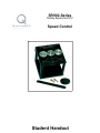
1
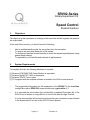
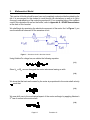
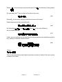
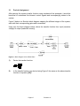
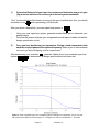
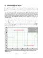
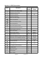
SRV02-Series
Rotary Experiment # 2
Speed Control
Student Handout
SRV02-Series
Rotary Experiment # 2
Speed Control
Student Handout
1.
Objectives
The objective in this experiment is to design a lead controller that will regulate the speed of
the output shaft.
At the end of this session, you should know the following:
•
•
•
•
How to mathematically model the servo plant from first principles.
To acquire an open-loop Bode plot of the system.
To design and simulate a lead controller to meet the required specifications (using
phase margin design).
To implement your controller and evaluate its performance.
2.
System Requirements
To complete this lab, the following hardware is required:
[1] Quanser UPM 2405/1503 Power Module or equivalent.
[1] Quanser MultiQ PCI / MQ3 or equivalent.
[1] Quanser SRV02-T servo plant.
[1] PC equipped with the required software as stated in the WinCon user manual.
•
The suggested configuration for this experiment is the SRV02-T in the Low-Gear
configuration with a UPM 1503 power module and a gain cable of 1.
•
It is assumed that the student has successfully completed Experiment #0 of the
SRV02 and is familiar in using WinCon to control the plant through Simulink.
•
It is also assumed that all the sensors and actuators are connected as per dictated
in the Experiment #0 as well as the SRV02 User’s Manual.
Page # 2
Revision: 01
3.
Mathematical Model
This section of the lab should be read over and completely understood before attending the
lab. It is encouraged for the student to work through the derivations as well as to get a
thorough understanding of the underlying mechanics. For a complete listing of the symbols
used in this derivation as well as the model, refer to Appendix A - SRV02 Nomenclature
at the back of this handout.
We shall begin by examining the electrical component of the motor first. In Figure 1, you
see the electrical schematic of the armature circuit.
Figure 1 - Armature circuit in the time-domain
Using Kirchhoff’s voltage law, we obtain the following equation:
[3.1]
Since Lm << Rm, we can disregard the motor inductance leaving us with:
[3.2]
We know that the back emf created by the motor is proportional to the motor shaft velocity
such that:
[3.3]
We now shift over to the mechanical aspect of the motor and begin by applying Newton’s
2nd law of motion to the motor shaft:
[3.4]
Page # 3
Revision: 01
Where
is the load torque seen thru the gears. And
is the efficiency of the gearbox.
We now apply the 2nd law of motion at the load of the motor:
[3.5]
Where Beq is the viscous damping coefficient as seen at the output.
Substituting [3.4] into [ 3.5], we are left with:
[3.6]
We know that
and
(where
is the motor efficiency),
we can re-write [3.6] as:
[3.7]
Finally, we can combine the electrical and mechanical equations by substituting [3.3] into
[3.7], yielding our desired transfer function:
[3.8]
Where:
This can be interpreted as the being the equivalent moment of inertia of the motor system
as seen at the output.
Page # 4
Revision: 01
3.1
Pre-Lab Assignment
After deriving the system transfer function using mechanical first principals, it would be
beneficial to understand the inherent control signals and accompanying states in the
system.
Figure 2 below is a Simulink block diagram mapping the different stages of the system,
each with their corresponding gains and conversions.
Using only the block diagram below, derive the transfer function from input (armature
voltage) to output (load shaft velocity).
Figure 2 - Block Diagram of the SRV02 Plant
1)
Derive the transfer function:
2)
Is the transfer function you derived using Figure 2 the same as the above transfer
function of equation [3.8]?
Page # 5
Revision: 01
4.
Lab Procedure
4.1
Wiring and Connections
The first task upon entering the lab is to ensure that the complete system is wired as
described in the SRV02 Experiment #0 - Introduction. If you are unsure of the wiring, please
refer to the SRV02 Manual or ask for assistance from a T.A. assigned to the lab. Now that
all the signals are connected properly, start-up MATLAB and start Simulink. You are now
ready to start the lab.
4.2
Controller Specifications
This lab requires you to design a Lead-Compensator to control the Servo plant with the
following specifications:
•
•
•
•
4.3
The system should have zero steady-state error (for a step input).
The system Bandwidth should be 100 rd/s (approximately 16 Hz).
The open-loop system should have a phase-margin of approximately 75
degrees.
The system should have no over-shoot (very minimal at the most).
Open Loop Characteristics
When designing a controller of a system in the frequency domain, it is necessary to first
study the open loop response of the system. In cases where the system cannot be modeled
from first principles (or the system is too complicated), an open loop Bode plot is acquired
by inputting a sinusoid of varying frequency and recording the magnitude and phase of the
corresponding output. In this case, our model is of first order and our model is sufficiently
accurate. The open-loop Bode plot to be used in the design will therefore be generated by
MATLAB using our plant model.
In order to achieve a zero steady-state error to a step input, our system must be of type 1.
By definition, a system is type 1 when it has a single pole located at the origin. We must
therefore introduce an integrator in the loop to track a step input with no steady-state error.
We now have the transfer function
function of:
4.4
with an integrator, yielding an open-loop transfer
Controller Parameters
After achieved the first criteria of zero steady-state error (with the integrator), the next task
should be to set the bandwidth of the system.
*Note: All relevant motor parameters can be found in Appendix A at the back of this handout or in
the SRV02 User Manual.
Page # 6
Revision: 01
1)
Generate a Bode plot of your open loop system and determine how much gain
(Kp) must be introduced to achieve your desired system bandwidth.
*Hint: Your bandwidth will be the zero crossing of the open-loop Bode plot. Also, you should
remember to use
when generating your Bode plot.
After you select a desired Kp, your new open-loop system is:
S
Using your new open-loop system, generate another Bode plot to determine your
phase-margin.
Calculate the amount of phase your compensator would require to add such that the
design specification is met.
S
2)
Once you have decided on your parameters, Design a Lead compensator that
adds the required phase at the required frequency. Refer to your in class material
on how to go about designing such a compensator.
After determining your controller
, generate a Bode plot of your complete open loop
system:
to determine if all design specifications have been met.
Figure 3 - Open loop Bode plot of the complete system including the compensator. As you can see,
the system has achieved a phase-margin of ~ 75 degrees as well as a bandwidth of ~ 100 rad/s
Page # 7
Revision: 01
Does your system meet the design specifications as seen in Figure 3? If you have not yet
met the specifications, you should go back and redesign your compensator. Most control
designs are iterative and will require fine-tuning to achieve the best control.
5.
Simulation & Implementation
5.1
Controller Simulation
If you are content with the controller and have met the required design specifications, you
are then ready to simulate your controller.
You must first run an M-file called “Setup_SRV02_Exp2.m”. This file initializes all the motor
parameters and gear ratios to the MATLAB workspace.
In Simulink, open a model called “s_tacho_lead.mdl”. This model includes the plant model
SRV-02 Plant Model (same as Figure 2), as a block in the final closed loop form. Use this
model to simulate your controller.
You can implement your controller by making sure the following variables are set in the
MATLAB workspace:
•
•
Desired_Kp - This variable should be set to the gain you had calculated to attain your
desired bandwidth (section 4.4).
Controller_NUM - This is the numerator of your compensator in decreasing orders
of s.
Controller_DEN - This is the compensator denominator in decreasing orders of s.
Ex:
If your controller transfer function was:
•
Controller_NUM = [2 1 -1]
Controller_DEN = [1 -3 5]
After setting the control parameters, you are now ready to simulate your design. Under the
simulation menu, choose start. Monitor the Simulated Velocity scope and compare the
signal to the Setpoint Input.
Looking at the system response (as well as the final Bode plot in section 4.4), you should
now have met all the design requirements. If you are content with your controller
performance, and are satisfied with your simulation, you are now ready to implement your
controller. Remember, if the simulated response is not desirable, you can easily re-iterate
your design process until you reach a satisfactory simulation.
Page # 8
Revision: 01
5.2
Implementation of the Controller
Open a Simulink model called “q_tacho_lead.mdl”. In this model, you will see 2 matching
loops. This will allow you to run the simulation as well as the actual plant simultaneously,
enabling you to note the difference in actual plant performance as opposed to the simulated
plant.
You must now build the model using the WinCon menu. Once it has compiled, you may
Start it using the WinCon server. The SRV-02 should now be tracking the command input.
Plot the Measured Velocity as well as the Setpoint and the Simulated Velocity. This is done
by clicking on the scope button in WinCon and choosing Measured Plant Velocity. Now you
must choose the Setpoint and the Simulated Velocity signals thru the Scope->File>Variables menu.
You should now be monitoring all 3 signals on the same plot. If your controller had been
designed to the above specifications and procedure, you should be seeing a response
similar to Figure 4 below.
*Note: Try adjusting the command input gain and take note of the response. DO NOT
exceed a command of 60 RPM for the high gear configuration or a command of 300 RPM
in the low gear configuration.
Figure 4 - Step response of the actual plant velocity (red) and the simulated velocity (blue) to an input
command (black).
Page # 9
Revision: 01
6.
Post Lab Questions & Report
After successfully designing and implementing your lead compensator, you should now
begin to document your report. This report should include:
I.
System characteristic Bode plots. Here you should include all Bode plots you
generated with all plots clearly labeled and documented.
II.
Design procedure. Clearly indicate all the steps you took in obtaining the final
controller. In this section, make clear reference to which Bode plots you used and
clearly label the system characteristic on each plot (i.e. phase margin).
III.
Any iterations in designing the controller should also be documented. (If your original
design did not meet the required specifications or if you wanted a better response).
IV.
The following plots as they are instrumental in measuring the quality of your design.
Make sure you include these plots and that they are labeled and documented:
•
•
A final open loop Bode plot of your complete system like the one seen in
Figure 3 of section 4.
A step response to your system including the actual and simulated velocities
as well as the input command. This should look similar to the Figure 4 of
section 5.
V.
Final remarks and conclusions as well as answers to the post lab questions.
6.1
Post Lab Questions
1)
Were there any design limitations or problems you encountered during the lab? If so,
how were these limitations overcome?
2)
Did the actual response of the system match directly to that of the simulated model?
From your understanding of the system, what could you theorize is the source of
these discrepancies and how would you improve them?
3)
If you were given the same speed control experiment again, would you choose a
lead compensator as a controller or would you use a different approach? Explain.
Page # 10
Revision: 01
Appendix - A: SRV02 Nomenclature
Symbol
Description
Vm
Armature circuit input voltage
Im
Armature circuit current
Rm
Armature resistance
Lm
Armature inductance
Eemf
Motor back-emf voltage
MATLAB
Variable
Nominal Value
SI Units
Rm
2.6
Motor shaft position
Motor shaft angular velocity
Load shaft position
Load shaft angular velocity
Tm
Torque generated by the motor
Tl
Torque applied at the load
Km
Back-emf constant
Km
0.00767
Kt
Motor-torque constant
Kt
0.00767
Jm
Motor moment of inertia
Jmotor
3.87 e-7
Jeq
Equivalent moment of inertia at the load
Jeq
9.31 e-4
Beq
Equivalent viscous damping coefficient
Beq
1.5 e-3
Kg
SRV02 system gear ratio (motor->load)
Kg
14 (14x1)
Gearbox efficiency
Eff_G
0.9
Motor efficiency
Eff_M
0.69
Undamped natural frequency
Wn
Damping ratio
zeta
Kp
Proportional gain
Kp
Kv
Velocity gain
Kv
Tp
Time to peak
Tp
Page # 11
Revision: 01