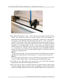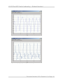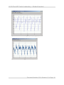
Download IP01_2 LFJC_SIP_LQR_Student_610

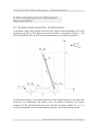
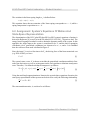
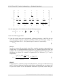
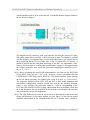
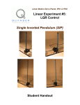
Linear Motion Servo Plants: IP01 or IP02
Linear Experiment #11:
LQR Control
Linear Flexible Joint Cart Plus
Single Inverted Pendulum (LFJC+SIP)
Student Handout
LFJC-Plus-SIP Control Laboratory – Student Handout
Table of Contents
1. Objectives............................................................................................................................1
2. Prerequisites.........................................................................................................................2
3. References............................................................................................................................2
4. Experimental Setup..............................................................................................................3
4.1. Main Components........................................................................................................3
4.2. Wiring..........................................................................................................................3
5. Controller Design Specifications.........................................................................................4
6. Pre-Lab Assignment: State-Space Representation..............................................................5
6.1. System Representation and Notations.........................................................................5
6.2. Assignment: System's Equations Of Motion And State-Space Representation...........6
7. In-Lab Procedure.................................................................................................................9
7.1. Experimental Setup......................................................................................................9
7.2. Design And Real-Time Implementation of a Linear Quadratic Regulator (LQR)......9
7.2.1. Objectives.............................................................................................................9
7.2.2. Experimental Procedure.......................................................................................9
Appendix A. Nomenclature...................................................................................................17
Document Number: 610 Š Revision: 01 Š Page: i
LFJC-Plus-SIP Control Laboratory – Student Handout
1. Objectives
The objective of the Linear Flexible
Joint Cart Plus Single Inverted
Pendulum (LFJC+SIP) experiment is to
design a control system to balance a
single inverted pendulum on a springdriven linear cart while minimizing the
spring deflection (i.e., oscillation). This
should only be achieved by controlling
the input (i.e. motorized) cart position.
The experiment consists of a system of
two carts sliding on an IP01 or IP02
track, as shown in Figure 1. While one
of the two carts is motorized and drives
the system (e.g. IP01 or IP02), the
second cart, a LFJC-PEN-E, is passive
and coupled to the first one through a
linear spring. The shafts of these
elements are coupled to a rack and
pinion mechanism in order to input the
driving force to the system and to
measure the two cart positions. An
single pendulum rod is mounted atop
the LFJC-PEN-E output cart and is free
to fall along the LFJC's axis of motion.
The single rod has its axis of rotation
perpendicular to the direction of motion
of the LFJ cart.
Figure 1 LFJC-PEN-E-Plus-SIP Coupled to an IP02
During the course of this experiment, you will become familiar with the design and
implementation of a full-state Linear Quadratic Regulator (LQR).
At the end of the session, you should know the following:
How to mathematically model the Linear Flexible Joint Cart Plus Single Inverted
Pendulum (LFJC+SIP) coupled to an IP01 or IP02 linear servo plant, using, for
example, Lagrangian mechanics or force analysis on free body diagrams.
How to obtain a state-space representation of the open-loop system.
How to design, simulate, and tune a LQR-based state-feedback controller satisfying
Document Number: 610 Š Revision: 01 Š Page: 1
LFJC-Plus-SIP Control Laboratory – Student Handout
the closed-loop system's desired design specifications.
How to use integral action to eliminate steady-state error.
How to implement your LQ Regulator in real-time and evaluate its actual
performance.
How to tune on-line and in real-time your LQR so that the actual linear-flexiblelinkage-cart system meets the closed-loop design requirements.
2. Prerequisites
To successfully carry out this laboratory, the prerequisites are:
i) To be familiar with your IP01 or IP02 main components (e.g. actuator, sensors), your
data acquisition card (e.g., Q8/Q4/MultiQ), and your power amplifier (e.g. UPM), as
described in References [2], [4], and [5].
ii) To be familiar with your Linear Flexible Joint Cart (LFJC-PEN-E) module, as
described in Reference [3].
iii) To have successfully completed the pre-laboratory described in Reference [1].
Students are therefore expected to be familiar in using WinCon to control and monitor
the plant in real-time and in designing their controller through Simulink.
iv) To be familiar with the complete wiring of your IP01 or IP02 servo plant, as per
dictated in Reference [2] and carried out in pre-laboratory [1].
v) To be familiar with the complete wiring of your LFJC-PEN-E module, as per dictated
in Reference [3].
vi) To be familiar with LQR design theory and working principles.
vii) To be familiar with FFT theory and working principles.
3. References
[1] IP01 and IP02 – Linear Experiment #0: Integration with WinCon – Student Handout.
[2] IP01 and IP02 User Manual.
[3] IP01 and IP02 – Linear Flexible Joint Cart Plus Single Inverted Pendulum
(LFJC+SIP) User Manual.
[4] Q8 User Manual.
[5] Universal Power Module User Manual.
[6] WinCon User Manual.
[7] IP01 and IP02 - Linear Experiment #1: PV Position Control – Student Handout.
[8] LFJC-Plus-SIP Dynamic Equations - Maple Worksheet.
Document Number: 610 Š Revision: 01 Š Page: 2
LFJC-Plus-SIP Control Laboratory – Student Handout
4. Experimental Setup
4.1. Main Components
To setup this experiment, the following hardware and software are required:
Power Module:
Quanser UPM 1503 / 2405, or equivalent.
Data Acquisition Board:
Quanser Q8 / Q4 / MultiQ PCI / MQ3, or equivalent.
Linear Motion Servo Plant: Quanser IP01 or IP02, as represented in Figure 1.
LFJC-PEN-E:
Quanser LFJC-PEN-E module, as seen in Figure 1.
Real-Time Control Software:
The WinCon-Simulink-RTX configuration, as
detailed in Reference [6], or equivalent.
For a complete and detailed description of the main components comprising this setup,
please refer to the manuals corresponding to your configuration.
4.2. Wiring
To wire up the system, please follow the default wiring procedures for your IP01 or IP02 as
well as for the LFJC-PEN-E module, as fully described in References [2] and [3],
respectively. When you are confident with your connections, you can power up the UPM.
Document Number: 610 Š Revision: 01 Š Page: 3
LFJC-Plus-SIP Control Laboratory – Student Handout
5. Controller Design Specifications
In the present laboratory (i.e. the pre-lab and in-lab sessions), you will design and
implement a control strategy based on the Linear Quadratic Regulator (LQR) scheme. As a
primary objective, the obtained optimal feedback gain vector, K, should allow you to keep
the single inverted pendulum balanced as well as to track the spring-driven load cart to a
desired position as quickly as possible while minimizing its overshoot, residual oscillation,
and steady-state error. The corresponding control effort should also be looked at and
minimized.
Please refer to your in-class notes, as needed, regarding the LQR design theory and the
corresponding implementation aspects of it. Generally speaking, the purpose of optimal
control is to allow for best trade-off between performance and cost of control.
Tune the LQR controlling the LFJC-Plus-SIP system in order to satisfy the following
design performance requirements:
1. Regulate the pendulum angle around its upright position and never exceed a ± 2.5degree-deflection from it, i.e.:
α ≤ 2.5 [ deg ]
2. While regulating both inverted pendulum and linear cart positions, minimize the
spring deflection, xs, such that:
xs ≤ 10.0 [ mm ]
3. Regulate the driving cart position, xc, so that it never exceeds the following:
xc ≤ 40.0 [ mm ]
4. Have no saturation in the system. In other words, the commanded motor input voltage
Vm (proportional to the control effort produced) should not make the power amplifier
(e.g. UPM) go into saturation.
As a remark, it can be seen that the previous design requirements bear on the system's three
outputs: xc, xs, and α. Therefore our inverted-pendulum-linear-cart system consists of three
outputs, for one input, Vm.
Document Number: 610 Š Revision: 01 Š Page: 4
LFJC-Plus-SIP Control Laboratory – Student Handout
6. Pre-Lab Assignment: State-Space
Representation
6.1. System Representation and Notations
A schematic of the Linear Flexible Joint Cart Plus Single Inverted Pendulum (LFJC+SIP)
mounted on an IP01 or IP02 linear-cart-and track system is represented in Figure 2. The
LFJC-plus-SIP-plus-IP01-or-IP02 system's nomenclature is provided in Appendix A.
Figure 2 Schematic of the LFJC-Plus-SIP System
As illustrated in Figure 2, the positive direction of linear displacement is to the right when
facing the cart. Furthermore, the positive sense of rotation is defined to be counterclockwise (CCW), when facing the linear cart. Also, the zero angle, modulus 2π, (i.e. α = 0
rad [2π]) corresponds to the inverted pendulum perfectly vertical and pointing upward.
Document Number: 610 Š Revision: 01 Š Page: 5
LFJC-Plus-SIP Control Laboratory – Student Handout
The variation in the linear spring length, xs, is defined below:
x s( t ) = x 2( t ) − x c( t )
This equation shows that an extension of the linear spring corresponds to xs > 0, while a
spring compression is equivalent to xs < 0.
6.2. Assignment: System's Equations Of Motion And
State-Space Representation
The determination of the LFJC-plus-SIP-plus-IP01-or-IP02 system's equations of motion is
derived in Reference [8] as well as in the file titled LFJC+SIP IP01_2 Equations.html. The
energy-based Lagrange's method is used to obtain the dynamic model of the system. In this
approach, the single input to the system is considered to be Fc, and the three Lagrangian
coordinates (a.k.a. generalized coordinates) are chosen to be: xc, xs, and α. It is reminded
that the reference frame used is defined in Figure 2.
Since the input U is set in a first time to be Fc, the driving force of the linear motorized cart
(e.g. IP01 or IP02), we have:
U = Fc
[1]
The system's state vector, X, is chosen to include the generalized coordinates and their firstorder time derivatives as well as an integrator on the cart's position to eliminate steady-state
error. Therefore, X is defined such that its transpose is as follows:
d
d
d
xc( t ) d t ⎤⎥⎥
X T = ⎡⎢⎢ xc( t ), xs( t ), α ( t ), x c( t ), xs( t ), α ( t ), ⌠
⎮
[2]
⎮
d
t
d
t
d
t
⌡
⎣
⎦
Using the small angle approximation to linearize the system's three equations of motion, the
state-space representation of that system can be derived to verify the following relationship:
∂
X=AX+BU
[3]
∂t
The state transition matrix, A, results to be as follows:
Document Number: 610 Š Revision: 01 Š Page: 6
LFJC-Plus-SIP Control Laboratory – Student Handout
⎡0
⎢
⎢0
⎢
⎢
⎢0
⎢
⎢
⎢
⎢
⎢0
⎢
⎢
A = ⎢⎢
⎢
⎢0
⎢
⎢
⎢
⎢
⎢
⎢0
⎢
⎢
⎢
⎢
⎢⎢
⎣1
0
0
1
0
0
0
0
0
1
0
0
0
0
0
1
0
0
Ks
−
Ks
Mc
−
−
−
0
Mc
Ks
Mp g
B eq
M c2
M c2
Mc
Ks
g ( M c2 + M p )
l p M c2
l p M c2
0
0
−
B eq
Mc
−
B eq2
M c2
B eq2
l p M c2
0
−
−
B eq2
−
M c2
B eq2
l p M c2
−
Bp
l p M c2
B p ( M c2 + M p )
0
Also the input matrix, B, is found to be with the following transpose:
1
1
⎡
−
0
0 ⎤⎥
0
0
B T = ⎢⎢ 0
⎥
Mc
Mc
⎣
⎦
2
M p l p M c2
0
0⎤
⎥
0⎥⎥
⎥
0⎥⎥
⎥
⎥
⎥
0⎥
⎥
⎥
⎥
⎥
⎥
0⎥⎥
⎥
⎥
⎥
⎥
0⎥⎥
⎥
⎥
⎥
⎥
0⎥⎦
[4]
[5]
Answer the following questions:
1. From the system's state-space representation, evaluate the matrices A and B for the case
where the system's input U is equal to the IP01 or IP02 cart's DC motor voltage Vm,
instead of the linear force Fc. The system's input U can now be expressed by:
U = Vm
[6]
Hint #1:
In order to convert the previously given force equation state-space representation to
voltage input, it is reminded that the driving force, Fc, generated by the DC motor and
acting on the cart through the motor pinion has already been determined in previous
laboratories. As shown for example in Equation [B.9] of Reference [7], Fc can be
expressed by:
2
d
ηg Kg ηm Kt Km ⎛⎜⎜ xc( t ) ⎞⎟⎟ η K η K V
⎝ dt
⎠+ g g m t m
[7]
Fc = −
2
Rm r mp
Rm r mp
Hint #2:
Evaluate matrices A and B by using the model parameter values given in References [2]
and [3]. Ask your laboratory instructor what system configuration you are going to use
in your in-lab session. In case no additional information is provided, assume that your
Document Number: 610 Š Revision: 01 Š Page: 7
LFJC-Plus-SIP Control Laboratory – Student Handout
system is composed of a LFJC-PEN-E module, together with its two additional masses,
mounted against an IP02 cart, atop of which its additional weight is also attached. The
long (i.e., 24-inch) single pendulum rod is also assumed.
2. Calculate the open-loop poles of the system. Is it stable? What is the type of the system?
What can you infer regarding the system's dynamic behaviour? Do you see the need for a
closed-loop controller? Explain.
Hint:
The characteristic equation of the open-loop system can be expressed by the equation
shown below:
det( s I − A ) = 0
[8]
where det() is the determinant function, s is the Laplace operator, and I the identity
matrix. Therefore, the system's open-loop poles can be seen as the eigenvalues of the
state-space matrix A.
Document Number: 610 Š Revision: 01 Š Page: 8
LFJC-Plus-SIP Control Laboratory – Student Handout
7. In-Lab Procedure
7.1. Experimental Setup
Even if you don't configure the experimental setup entirely yourself, you should be at least
completely familiar with it and understand it. If in doubt, refer to References [1], [2], [3],
[4], [5], and/or [6].
The first task upon entering the lab is to ensure that the complete system is wired as fully
described in References [2] and [3]. You should have become familiar with the complete
wiring and connections of your IP01 or IP02 system during the preparatory session
described in Reference [1]. If you are still unsure of the wiring, please ask for assistance
from the Teaching Assistant assigned to the lab. When you are confident with your
connections, you can power up the UPM. You are now ready to begin the lab.
7.2. Design And Real-Time Implementation of a Linear
Quadratic Regulator (LQR)
7.2.1. Objectives
To use the obtained LFJC-plus-SIP-plus-IP01-or-IP02 state-space representation to
design the following kind of state-feedback controller: Linear Quadratic Regulator
(LQR).
To implement with WinCon a real-time LQR for your actual LFJC-plus-SIP-plusIP01-or-IP02 plant.
To tune and implement the LQ Regulator on the actual system and in real-time with
WinCon.
To assess from the actual system response whether the closed-loop design
requirements are satisfied.
7.2.2. Experimental Procedure
Please follow the steps described below.
Step1. If you have not done so yet, you can start-up MATLAB now. Depending on your
system
configuration,
open
the
Simulink
model
file
of
type
q_lqr_lfjce_sip_YY_ZZ.mdl, where YY for either 'ip01' or 'ip02', and ZZ for either for
'q8', 'q4', 'mq3', 'mqp', or 'nie'. Ask the TA assigned to this lab if you are unsure
Document Number: 610 Š Revision: 01 Š Page: 9
LFJC-Plus-SIP Control Laboratory – Student Handout
which Simulink model is to be used in the lab. You should obtain a diagram similar to
the one shown in Figure 3.
Figure 3 Actual Implementation of the LQR Closed-Loop System For The LFJC-plus-SIP-plus-IP02
The diagram directly interfaces with your hardware and runs the actual LFJC-plusSIP system connected to your IP01 or IP02 linear servo plant. To familiarize yourself
with the diagram, it is suggested that you open both subsystems to get a better idea of
their composing blocks as well as take note of the I/O connections. Of interest, it
should be noticed that the subsystem interfacing to the IP01 cart implements a Bias
Removal block in order to set both initial potentiometer voltages to zero upon starting
the real-time controller. Also, check that your model sampling time should be set to 1
ms, i.e. Ts = 10-3 s.
Step2. Before beginning the actual LQR implementation, you must run the MATLAB
script called setup_lab_ip01_2_lfjc_sip.m. However, ensure beforehand that the
CONTROLLER_TYPE flag is set to 'MANUAL'. This mode initializes, before starting
on-line the tuning procedure, the optimal gain vector K to zero, i.e. [0,0,0,0,0,0,0].
The script also initializes all the LFJC, SIP, and IP01 or IP02 model parameters and
user-defined configuration variables needed and used by the Simulink diagram.
Lastly, it also calculates the state-space matrices, A and B, corresponding to the
LFJC-plus-SIP-plus-IP01-or-IP02 system configuration that you defined. Check that
the A and B matrices thus set in the MATLAB workspace correspond to the ones that
you evaluated in your pre-lab assignment.
Step3. The LQR feedback gain vector K now needs to be determined so that the desired
design specifications, as previously defined, are met. Since it is used by the actual
controller implemented in the Simulink model file, the 7-element vector variable K
Document Number: 610 Š Revision: 01 Š Page: 10
LFJC-Plus-SIP Control Laboratory – Student Handout
must also be set in the MATLAB workspace. Using the MATLAB 'lqr' function,
calculate the optimal gain vector K corresponding to the two following weighting
matrices Q and R:
0
0 0 0 0
0⎤
⎡⎢ 4000
⎥
⎢⎢
0 500
0 0 0 0
0 ⎥⎥
⎥
⎢
⎢⎢
0
0 3000 0 0 0
0 ⎥⎥
R = [1.0 ]
0
0
0 0 0 0
0 ⎥⎥
Q = ⎢⎢
[9]
⎥
⎢⎢
⎥
0
0
0 0 0 0
0⎥
⎢⎢
⎥
⎢
0
0
0 0 0 0
0 ⎥⎥
⎢⎢
⎥
⎢
0
0
0 0 0 0 100 ⎥⎦
⎣
CAUTION:
Once K has been calculated, have your lab assistant check your controller gain
values. DO NOT proceed to the next step without his or her approval.
Step4. Calculate the location of the corresponding closed-loop poles. Compare them to
the location of the open-loop poles found in your pre-lab assignment.
Hint #1:
You can use the MATLAB function 'eig' to determine the eigenvalues of the closedloop state-space matrix.
Hint #2:
The closed-loop state-space matrix can be expressed as: A-B*K.
Step5. You are now ready to build the real-time code corresponding to your diagram, by
using the WinCon | Build option from the Simulink menu bar. After successful
compilation and download to the WinCon Client, you should be able to use WinCon
Server to run in real-time your actual system. However, before doing so, manually
move your LFJC-plus-IP01-or-IP02 cart system to the middle of the track (i.e.,
around the mid-stroke position) and make sure that it is free to move on both
sides. Additionally, ensure that the pendulum is free to rotate over its full
rotational range (±360º) from anywhere within the LFJ cart's full linear range of
motion. Before starting the real-time controller, also follow the starting procedure for
the inverted pendulum, as described in the following Step.
Step6. Inverted Pendulum Starting Procedure. One important consideration to bear in
mind for the pendulum starting procedure is that encoders take their initial position
reading as zero when the real-time code is started. In our linearized model, it is
reminded that the zero pendulum angle corresponds to a perfectly upright position.
The starting procedure described hereafter finds the exact vertical position from the
pendulum hanging straight down, at rest, in front of the LFJC linear cart.
Document Number: 610 Š Revision: 01 Š Page: 11
LFJC-Plus-SIP Control Laboratory – Student Handout
Step7. The starting procedure consists first of letting the pendulum come to perfect
rest in the gantry configuration, so that it is hanging straight down. This is
illustrated in Figure 4.
Figure 4 LFJC-plus-SIP-plus-IP02 Starting Position
Then, the real-time code can be started so that the exact ±π-radian angle is precisely
known. To do this, click on the START/STOP button of the WinCon Server window.
Finally, manually rotate the pendulum to its upright position. The LQR, initially
turned off by the start-up logic implemented in the controller model file, should
automatically kick in and become enabled once the pendulum is completely inverted
(i.e., its angle reached zero). The controller becomes effective only once the vertical
equilibrium point is reached. At this stage, you can let the inverted pendulum go
without trying to help it any further. Your LQR real-time controller should now
command the IP01 or IP02 cart position so that the system regulates a constant
setpoint while maintaining the inverted pendulum balanced. This is depicted in Figure
5.
Document Number: 610 Š Revision: 01 Š Page: 12
LFJC-Plus-SIP Control Laboratory – Student Handout
Figure 5 LFJC-plus-SIP-plus-IP02 Balancing Position
Step8. Open the three sinks xc (mm), xs (mm), and alpha (deg) in three separate WinCon
Scopes. You should also check the system's control effort and saturation, as
mentioned in the design specifications, by opening the V Command (V) scope located,
for example, in the following subsystem path: LFJC-PEN-E + IP02: Actual Plant Q8/IP02 - Q8/. On the xc (mm) scope, you should now be able to monitor on-line, as
the IP01 or IP02 motorized cart moves and drives the LFJC, the actual cart position
regulating at its starting position. On the xs (mm) scope, you should be able to
monitor on-the-fly, as both linear cart moves, the actual resulting spring elongation
(i.e., compression or extension). On the alpha (deg) scope, you should be able to
monitor in real-time the actual inverted pendulum angle as it fluctuates about the
vertical axis at any given time.
Hint #1:
To open a WinCon Scope, click on the Scope button of the WinCon Server window
and choose the display that you want to open (e.g., xc (mm)) from the selection list.
Hint #2:
For a better signal visualization, you can set the WinCon scope buffer to 20 seconds.
To do so, use the Update | Buffer... menu item from the desired WinCon scope.
Step9. What are your observations at this point? Does your actual LQR closed-loop
implementation meet the desired design specifications?
Step10. If it does not, then you should re-iterate the controller design by finely tuning
the LQR weighting matrices, Q and R, and re-computing K so that the final system
satisfies the design requirements. Iterate your manual LQR tuning as many times as
Document Number: 610 Š Revision: 01 Š Page: 13
LFJC-Plus-SIP Control Laboratory – Student Handout
necessary so that your actual system's performance meets the desired design
specifications. Also remember to avoid system saturation by monitoring the
corresponding control effort spent, by means of the V Command (V) scope. If you are
still unable to achieve the required performance level, ask your T.A. for advice.
Step11. Once your results are in agreement with the closed-loop requirements, they
should look similar to those displayed in Figures 6, 7, 8, and 9, below. Also ensure
that the actual commanded motor input voltage Vm (which is proportional to the
actual control effort produced) does not go into saturation, as listed as part of the
requirements. As an example, an acceptable command voltage Vm is illustrated in
Figure 9. More specifically, it can be observed in Figure 9 that no saturation occurs in
the system and that the commanded motor input voltage is always such that:
V m ≤ 4.0 [ V ]
Step12. Include the corresponding plots (e.g., screen captures of WinCon Scopes) in
your lab report to support your observations. You should at least include the WinCon
plots, that you obtained, equivalent to Figures 6, 7, 8, and 9. Also include your final
Q and R matrices as well as the resulting LQR gain vector K. Ensure to properly
document all your results and observations before leaving the laboratory session.
Step13. Remember that there is no such thing as a perfect model. Specifically discuss in
your lab report how your actual linear cart positions and inverted pendulum angle
compare to their respective theoretical values? Outline the most prominent
differences between the theoretical and actual responses. Is there any discrepancy in
the results? If so, find some of the possible reasons.
Document Number: 610 Š Revision: 01 Š Page: 14
LFJC-Plus-SIP Control Laboratory – Student Handout
Figure 6 Actual Motorized Cart (IP02) Response: xc (mm) Scope
Figure 7 Actual Spring Elongation Response: xs (mm) Scope
Document Number: 610 Š Revision: 01 Š Page: 15
LFJC-Plus-SIP Control Laboratory – Student Handout
Figure 8 Actual Inverted Pendulum Angle Response: alpha (deg) Scope
Figure 9 Actual Command Voltage: V Command (V) Scope
Document Number: 610 Š Revision: 01 Š Page: 16
LFJC-Plus-SIP Control Laboratory – Student Handout
Appendix A. Nomenclature
Table A.1, below, provides a complete listing of the symbols and notations used in the IP01
and IP02 mathematical modelling, as presented in this laboratory. The numerical values of
the system parameters can be found in Reference [2].
Symbol
Description
MATLAB
Notation
Vm
Motor Armature Voltage
Vm
Im
Motor Armature Current
Im
Rm
Motor Armature Resistance
Rm
Kt
Motor Torque Constant
Kt
ηm
Motor Efficiency
Km
Back-ElectroMotive-Force (EMF) Constant
Km
Jm
Rotor Moment of Inertia
Jm
Kg
Planetary Gearbox Gear Ratio
Kg
ηg
Planetary Gearbox Efficiency
Eff_g
Mc
Lumped Mass of the IP01 or IP02 Cart System, including
the Rotor Inertia
rmp
Motor Pinion Radius
r_mp
Beq
Equivalent Viscous Damping Coefficient as seen at the
Motor Pinion
Beq
Fc
Cart Driving Force Produced by the Motor
xc
Motorized Cart Linear Position
xc
∂
x
∂t c
Motorized Cart Linear Velocity
xc_dot
Time Integration of the Motorized Cart Linear Position
xc_int
⌠
xc d t
⎮
⎮
⌡
Eff_m
Mc
Table A.1 IP01 and IP02 Model Nomenclature
Table A.2, below, provides a complete listing of the symbols and notations used in the
mathematical modelling of the Linear Flexible Joint Cart Plus Single Inverted Pendulum
(LFJC+SIP) system, as presented in this laboratory. The numerical values of the LFJC-
Document Number: 610 Š Revision: 01 Š Page: 17
LFJC-Plus-SIP Control Laboratory – Student Handout
PEN-E-plus-SIP system parameters can be found in Reference [3].
Symbol
Description
Mc2
Mass of the Load Cart System
Ks
Linear Spring Stiffness Constant
Beq2
Equivalent Viscous Damping Coefficient as seen at the
Load Cart Position Pinion
MATLAB
Notation
Mc2
Ks
Beq2
x2
Load Cart Linear Position
x2
∂
x
∂t 2
Load Cart Linear Velocity
x2_dot
xs
Linear Spring Elongation
xs
∂
x
∂t s
α
Linear Spring Elongation Velocity
xs_dot
Pendulum Angle From the Upright Position
alpha
∂
α
∂t
Pendulum Angular Velocity
Mp
Pendulum Mass (with T-fitting)
Mp
Bp
Pendulum Viscous Damping Coefficient as seen at the
Pendulum Axis
Bp
Lp
Pendulum Full Length (from Pivot to Tip)
Lp
lp
Pendulum Length from Pivot to Center Of Gravity
lp
xp
x-coordinate of the Pendulum Centre Of Gravity
yp
y-coordinate of the Pendulum Centre Of Gravity
alpha_dot
Table A.2 LFJC-Plus-SIP System Model Nomenclature
Table A.3, below, provides a complete listing of the symbols and notations used in the LQR
controller design, as presented in this laboratory.
Document Number: 610 Š Revision: 01 Š Page: 18
LFJC-Plus-SIP Control Laboratory – Student Handout
Symbol
Description
A, B, C, D State-Space Matrices of the LFJC-plus-SIP-plus-IP01or-IP02 System
MATLAB
Notation
A, B, C, D
X
State Vector
X
Y
System Output Vector
Y
K
Optimal Feedback Gain Vector
K
U
Control Signal (a.k.a. System Input)
Q
Non-Negative Definite Hermitian Matrix
Q
R
Positive-Definite Hermitian Matrix
R
t
Continuous Time
dx
Variation in the Linear Spring Length
dx
Table A.3 LQR Controller Nomenclature
Document Number: 610 Š Revision: 01 Š Page: 19