Download Flexible Link

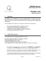
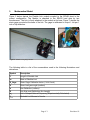
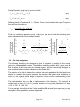
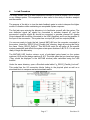
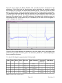
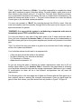
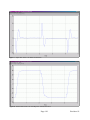
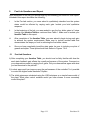
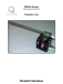
SRV02-Series
Rotary Experiment # 5
Flexible Link
Student Handout
SRV02-Series
Rotary Experiment # 5
Flexible Link
Student Handout
1.
Objectives
The objective in this experiment is to tune a state-feedback controller for the rotary
flexible link module. The final controller should allow the user to command a desired tip
angle position. The controller should eliminate the link's vibrations while maintaining a
fast response.
Upon completion of the exercise, you should have experience in the following:
•
•
•
•
•
2.
How to mathematically model the Flexible Link system.
To linearize the model about an operating point.
To dampen the arm vibrations by tuning the controller.
To design and simulate a WinCon controller for the system.
How to design an optimal LQR controller.
System Requirements
To complete this Lab, the following hardware is required:
[1] Quanser UPM 2405/1503 Power Module or equivalent.
[1] Quanser MultiQ PCI / MQ3 or equivalent.
[1] Quanser SRV02-E(T) servo plant.
[1] Quanser FLEXGAGE– Rotary Flexible Link Module.
[1] PC equipped with the required software as stated in the WinCon user manual.
•
The required configuration of this experiment is the SRV02-E(T) in the High-Gear
configuration with a UPM 2405 power module and a suggested gain cable of 1.
•
It is assumed that the student has successfully completed Experiment #0 of the
SRV02 and is familiar in using WinCon to control the plant through Simulink.
•
It is also assumed that all the sensors and actuators are connected as per dictated
in the SRV02 User Manual and the Rotary Flexible Link User Manual.
Page # 2
Revision: 01
3.
Mathematical Model
Figure 2 below depicts the Flexible Link module coupled to the SRV02 plant in the
correct configuration. The Module is attached to the SRV02 load gear by two
thumbscrews. The Link is firmly attached to the module at its base. Figure 1 depicts the
strain gage mounted at the base of the link. The gage is calibrated to output 1 volt per 1
inch of tip deflection.
Figure 1 - Strain Gage
Figure 2 - SRV02 w/ FlegGage Module
The following table is a list of the nomenclature used is the following illustrations and
derivations.
Symbol
Description
L
Length of Flexible Link
m
Mass of Flexible Link
K_Gage
Strain Gage Calibration factor (1 Volt / Inch)
θ
Servo load gear angle (radians)
α
Arm Deflection (radians)
D
Link End-point Deflection (Arc Length)
ωc
Link's Damped Natural Frequency (Experimentally Calculated)
JLink
Modeled Link Moment of Inertia
Page # 3
Revision: 01
Figure 3 - Schematic of Flexible Link Module
Figure 3 depicts the flexible link at a given deflection resulting in an end-point
displacement of D. The stain-gage is calibrated such that it outputs 1 volt per 1 inch
deflection of D resulting in the following equation:
=
D
L
[3.1]
To get a complete model of a flexible link is beyond the scope of this laboratory. In
controlling the tip of the link, it is sufficient to use a simplified model that will adequately
describe the motion of the endpoint. Figure 4 below depicts the simplified model:
Figure 4 - Simple Flexible Link Model
From Figure 4, the equation of a rotary spring is:
J Link ̈=−K Stiff 
[3.2]
Page # 4
Revision: 01
To get an estimation of the the modeled stiffness (Kstiff), we fixed the clamped end of the
link and set an initial condition of alpha and measured the link's damped natural
frequency. With any given oscillation system, we have the following relation:
̈=− 2c 
[3.3]
Combining equations [3.2] & [3.3], we are left with the following expression:
K Stiff = 2c J Link
[3.4]
Were the Link is modeled as a rod rotating about its endpoint with moment of inertia:
J Link =
3.1
M L2
3
[3.5]
Deriving The System Dynamic Equations
Now that we have developed a simple model for the Link, the system dynamic equations
can be obtained using the Euler-Lagrange formulation. We obtain the Potential and
Kinetic energies in our system as:
Potential Energy - The only potential energy in the system is in the spring:
1
V =P.E.Spring = K Stiff  2
2
[3.6]
Kinetic Energy - The Kinetic Energies in the system arise from the moving hub and
flexible link:
1
1
2
2
T =K.E. HubK.E. Link = J eq ˙  J Link  ̇̇
2
2
[3.7]
Forming the Lagrangian:
1
1
1
L=T −V = J eq ˙2 J Link  ̇̇2− K Stiff  2
2
2
2
[3.8]
Our 2 generalized co-ordinates are θ and α. We therefore have 2 equations:

t

t
 
 
L
L
=T output −Beq ̇
−
 ̇

[3.9]
L
L
−
=0
 ̇

[3.10]
Page # 5
Revision: 01
Solving Equations [3.9] & [3.10], we are left with :
J eq ̈J Arm  ̈̈=T output−Beq ̇
[3.11]
J Arm  ̈̈K Stiff =0
[3.12]
Referring back to Experiment # 1 – Position Control, we know that the output Torque on
the load from the motor is:
T output=
m  g K t K g V m−K g K m ̇
[3.13]
Rm
Finally, by combining equations [3.11], [3.12] & [3.13], we are left with the following statespace representation of the complete system:
[]
[
0
0
0
0
̇
K Stiff
̇
= 0
J eq
̈
̈
−K Stiff J eq J Arm 
0
J eq J Arm
3.2
1
0
− m  g K t K m K 2g Beq Rm
J eq Rm
m  g K t K m K 2g Beq Rm
J eq Rm
][ ] [ ]
0
1
0
0
0
0
m  g K t K g



J eq Rm
̇
−m  g K t K g
̇
Vm
J eq Rm
Pre Lab Assignment
The following laboratory was designed to give the student an insight into the various
gains in a state-feedback system. The student is initially provided with a gain vector k
that will place the link end-point at a desired location, but was intentionally designed to
also introduce higher modes of vibrations in the flexible link.
The purpose of the lab is to have the students vary each gain about its initial point in an
attempt to maintain the system response but dampen the higher mode vibrations. In
doing so, the student should begin to develop a more intuitive understanding of the
various state-feedback gains.
The state-feedback law u = -kx is implemented in this laboratory. The controller is
initialize with 4 gains (k1, k2, k3, k4) and the student is to vary each parameter in 5 steps
( 0.5k , 0.75k , k , 1.5k , 2k ).
For the pre-lab, what effect on the 2 state variables (θ & α) would you expect as you vary
each gain? Only a qualitative answer is required.
Page # 6
Revision: 01
4.
In Lab Procedure
The rotary flexible Link is an ideal experiment intended to model a flexible Link on a robot
or any linkage system. This experiment is also useful in the study of vibration analysis
and resonance.
The purpose of the lab is to tune the state-feedback gains in order to dampen the higher
modes of vibrations while maintaining an acceptable system response.
The first task upon entering the laboratory is to familiarize yourself with the system. The
arm deflection signal (α) should be connected to encoder channel #1 and the
servomotor's position signal (θ) should be connected to encoder channel #0. Analog
Output channel #0 should be connected to the UPM (Amplifier) and from the amplifier to
the input of the servomotor. This system has one input (Vm) and two outputs (θ & α).
You are now ready to begin the lab. Launch MATLAB from the computer connected to
the system. Under the “SRV02_Exp5_Flexible Link” directory, begin by running the file by
the name “Setup_SRV02_Exp5.m”. This MATLAB script file will setup all the specific
system parameters and will set the system state-space matrices A,B,C & D. You are now
ready to begin the laboratory.
The MATLAB LQR function returns a set of calculated gains based on the system
matrices A & B and the design matrices Q & R. The initial gains that you have been given
(They should be displayed in the MATLAB window) were calculated using the LQR
method.
Under the same directory, open a Simulink model called “q_SRV02_Flexible_Link.mdl”.
This model has the I/O connection blocks linking to the physical plant as well as a
simulated block to compare real and simulated results.
Figure 5 - Flexible Link Controller
Page # 7
Revision: 01
Figure 5 above depicts the Rotary Flexible Link controller we have developed for this
experiment. Notice that both the actual system and a simulation are running in parallel
thus allowing us to compare the actual and simulated results. Take note of the four slider
gains in the controller. These are the gains that you will be Tuning during this experiment.
The simulation running in parallel with the controller is of the simplified linear model. The
controller gains that you will be using as the base of this experiment were calculated
based on this simple model. Using this technique, the higher-order vibrations were not
anticipated and that is the reason why it is necessary for the user to tune the gains in
order to dampen the vibrations.
Figure 6 - Higher Order Vibrations
Figure 6 Above clearly displays the vibrations in the link (Alpha) due to the higher order
modes being excited. The main goal of this laboratory would be to sufficiently dampen
these unwanted vibrations.
You should first begin by preparing the following table:
Slider1 Slider2 Slider3 Slider4 Rise time
Alpha Vibrations % Overshoot
(Gamma)
Alpha Range
0.5
1
1
1
Slower
More
0
- 3.5º < α < 3.5º
0.75
1
1
1
Slower
Unchanged
0
- 6º < α < 6º
1
1
1
1
Same
Unchanged
0
- 8º < α < 8º
1.5
1
1
1
Faster
Less
15.00%
- 10º < α < 10º
2
1
1
1
Faster
Less
35.00%
- 12º < α < 12º
Table 1 - Iteration Table : Sample Entries
Page # 8
Revision: 01
Table 1 shows the 5 iterations of Slider1. You will be responsible to complete the above
table with 5 iterations for each of the other sliders. For each iteration, make sure to set all
other sliders to their default value of 1. For the Rise Time and Alpha Vibrations columns,
only a quantitative observation will suffice. Be sure to compare each observation to the
default set where each slider is set to 1. The goal of this excerise is to notice the effects
of each gain on the individual system parameters.
You may now proceed to “Build” the controller through the WinCon menu. After the
code has compiled, start the controller through WinCon and open up two scopes; one for
alpha and another for gamma.
*WARNING: If at any point the system is not behaving as expected, make sure to
immediately press STOP on the WinCon server.
You may now begin to vary each of the slider gains in the 5 steps mentioned above.
Once you have completed the Iteration Table, you should have a good understanding of
the effects each gain has on the system response and should now proceed to tune each
gain.
*Hint: You should be using your table as a guide to pick the best set of slider settings to
achieve the system requirements.
Your final slider values should result in a response with:
•
•
•
•
A fast rise-time (should be similar to the default).
No Alpha Vibrations (very minimal at the least).
0 % Overshoot on Gamma.
Alpha should not exceed ± 10°.
As you are tuning the gains to achieve the system requirements, make sure to fill out
another table similar to your Iteration Table to document the steps taken at achieving
your final slider values that best meet the system requirements. Make sure to try a variety
of combinations as there will be a few different configurations that will meet the
requirements.
The following plots on the next page are of Alpha and Gamma with the Slide gains set to
their optimum values in meeting the controller requirements. Once you have tuned the
gains to their final values, your plots should look very similar to Figure 7 & Figure 8.
Page # 9
Revision: 01
Figure 7 - Alpha Plot: Notice the Reduced Vibrations
Figure 8 - Gamma Plot: Notice the Fast Response without Overshoot
Page # 10
Revision: 01
5.
Post Lab Questions and Report
Upon completion of the lab, you should begin by documenting your work into a lab report.
Included in this report should be the following:
i.
In the Pre-Lab section, you were asked to qualitatively describe how the system
states would be effected by varying each gain. Include your brief qualitative
response.
ii.
In the beginning of the lab, you were asked to vary the four slider gains in 5 steps
forming your Iteration Table as continued from Table 1. Make sure to include your
Iteration Table in this report.
iii.
After completion of the Iteration Table, you were asked to begin tuning each gain
to achieve the system requirements. Make sure to include another table that
demonstrates the steps you took in achieving the final slider values.
iv.
Once you have completely tuned the state gains, be sure to include your plots of
gamma and alpha. These plots should look similar to Figures 7 & 8.
5.1
Post Lab Questions
1) After completing your Iteration Table, you should now be fairly familiar with how the
each state-feedback gain effects the overall performance of the system. Comment on
your observations made by varying the 4 gains. Did your observations agree with what
you had theorized in the pre-lab?
2) In what ways could you improve upon the performance of the controller? Is it possible
to control the higher mode vibrations? Explain.
3) The initial gains were calculated using the LQR technique on a simple linear model of
the plant. What other control methods would you have chosen to more accurately
control this plant?
Page # 11
Revision: 01