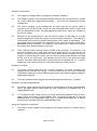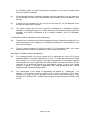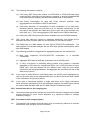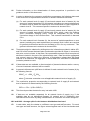
Download CDCM User Manual – May 2012

User manual for CDCM Model 100
May 2012, revision 3275
13/07/201213/07/2012Page 1 of 36Page 1 of 36
energynetworks.org
Contents
Overview .............................................................................................................................. 3
Guidance on asset models ................................................................................................. 7
General costing guidance for asset models........................................................................... 9
Network model ...................................................................................................................... 9
Service models ................................................................................................................... 11
Input data tables ............................................................................................................... 15
1000. Company name, charging year and model version ................................................... 15
1010. Financial and general assumptions .......................................................................... 15
1017. Diversity allowance between top and bottom of network level .................................. 15
1018. Proportion of relevant load going through 132kV/HV direct transformation ............... 16
1019. Network model GSP demand (MW) ......................................................................... 16
1020. Gross asset cost by network level (£) ....................................................................... 16
1022. LV service model asset cost (£) ............................................................................... 16
1023. HV service model asset cost (£) ............................................................................... 16
1025. Matrix of applicability of LV service models to tariffs with fixed charges.................... 17
1026. Matrix of applicability of LV service models to unmetered tariffs ............................... 17
1028. Matrix of applicability of HV service models to tariffs with fixed charges ................... 17
1032. Loss adjustment factors to transmission ................................................................... 17
1037. Embedded network (LDNO) discounts ..................................................................... 17
1041. Load profile data for demand users: coincidence factor; load factor ......................... 17
1053. Volume forecasts for the charging year .................................................................... 18
1055. Transmission exit charges (£/year)........................................................................... 18
1059. Other expenditure .................................................................................................... 19
1060. Customer contributions under current connection charging policy ............................ 19
1061 and 1062. Average split of units between distribution time band ............................... 20
1068. Typical annual hours by distribution time band ......................................................... 21
1069. Peaking probabilities by network level ...................................................................... 21
1076. Target revenue ......................................................................................................... 22
1092. Average kVAr by kVA, by network level.................................................................... 23
1201. Current tariff information ........................................................................................... 23
Calculation sheets ............................................................................................................ 24
LAFs — Loss adjustment factors and network use matrices ............................................... 24
DRM — Network model ...................................................................................................... 25
SM — Service models......................................................................................................... 25
Loads — Load characteristics ............................................................................................. 26
Multi — Load characteristics for multiple unit rates ............................................................. 26
SMD — Forecast simultaneous maximum load ................................................................... 27
AMD — Forecast aggregate maximum load ........................................................................ 28
Otex — Other expenditure .................................................................................................. 29
Contrib — Customer contributions ...................................................................................... 31
Yard — Yardsticks .............................................................................................................. 31
Standing — Allocation to standing charges ......................................................................... 32
NHH — Standing charges as fixed charges ........................................................................ 32
Reactive — Reactive power unit charges ............................................................................ 33
Aggreg — Aggregation........................................................................................................ 34
Revenue — Revenue shortfall or surplus ............................................................................ 34
Scaler — Revenue matching............................................................................................... 35
Adjust — Tariff component adjustment and rounding .......................................................... 36
Page 2 of 36
Overview
1.
This user manual accompanies the spreadsheet model that is used to implement the
Common Distribution Charging Methodology (CDCM) for electricity distribution
networks in Great Britain (the CDCM Model). The CDCM is contained within
Schedule 16 of DCUSA and the current model version number is referred to in
paragraph 3 of Schedule 16. This user manual is based on version 100 of the model
which was published on 1st April 2010.
2.
The CDCM model may be updated following a DCUSA change proposal. Users of
the CDCM Model should check that they are using the most up to date version of the
model by checking the current version of DCUSA at the DCUSA website:
http://www.dcusa.co.uk/Public/DCUSADocuments.aspx?s=c.
3.
Figure 1, reproduced from the CDCM statement, shows the main steps in the
methodology and model. Figure 2 gives an overview of relationships between the
main elements of the model.
Figure 1 Overview of main steps and data flows
Page 3 of 36
Figure 2 Overview of the relationship between elements of the model
Sheets
4.
Sheets in the workbook have been given very short abbreviated names. This is to
make the best use of screen space given the way in which Microsoft Excel displays
information. A proper title appears at the top of each sheet.
5.
Figures 3 and 4 are maps of the calculation sheets in the model workbook.
Figure 3 Step 2 sheets in the workbook (data flow from left to right)
Figure 4 Step 3 sheets in the workbook (data flow from left to right)
Page 4 of 36
Tables
6.
Each sheet is structured as a list of data tables, to be read from top to bottom — like
a book.
7.
Each of these data tables has a four-digit table number. Numbers that start with 10
are manually assigned for input data tables and do not change from version to
version. Other table numbers are assigned when the model is built and may vary
when the model is changed or different options are selected.
Hyperlinks in the workbook
8.
The tables in the model are listed in the overview sheet, with hyperlinks to the data.
Links to the source data for each calculation are shown above each calculation table.
9.
The Forward and Back buttons on Microsoft Excel’s Web toolbar can be useful when
navigating around the workbook using these hyperlinks. For example, to go back to
where you were before clicking a hyperlink, use the Back button.
10.
To show the Web toolbar in Microsoft Excel 2000–2004, select Web from Toolbars
from the View menu (details may vary depending on the Excel version). The Web
toolbar has been removed from Microsoft Excel 2007, but the Back and Forward
buttons can be added to the Quick Access Toolbar instead.
11.
Links do not work well if the model is displayed within a web browser. To get the full
functionality, save the model as a file and open it in Microsoft Excel or compatible
software.
Technologies and dependencies
12.
The model is implemented as a stand-alone Microsoft Excel workbook in Excel
1997–2003 file format. No software other than Microsoft Excel 1997 or above (or
compatible software) is needed to operate the model.
13.
The model relies on standard spreadsheet formulae. It does not use any macros,
Visual Basic for Application, pivot tables, solver, goal seek, or array formulae.
14.
The workbook is produced by a computer programme in the programming language
Perl 5. This programme can be run on a personal computer or as a web service, and
can generate versions of the models with different tariffs or allocation rules.
Overview sheet
15.
The overview sheet (Overview) lists the data tables in the workbook.
Input sheet
16.
The input data sheet (Input) contains all the input data for the model.
Tariff sheets
17.
The tariff sheet (Tariffs) summarises the final tariffs.
Page 5 of 36
Additional output sheets
18.
The summary sheet (Summary) gives a copy of the tariffs, average revenue per unit
and average revenue per user for each tariff, and a summary of options and
assumptions used in the model.
19.
Tariff matrices are provided on the M-ATW sheet. Tariff matrices show the tariff
components of the final tariffs and their decomposition into the various elements of
cost and revenue in a form that can be easily read and printed.
20.
The revenue matrix sheet (M-Rev) shows the revenues raised in respect of each end
user type and each element of cost or revenue in the model.
21.
The comparison sheets (CData and CTables) attempt an indicative comparison
between current and proposed all-the-way tariffs, and between all-the-way and
LDNO tariffs.
22.
All these additional output sheets are for information only. They can be removed or
modified without effect on the rest of the calculations.
Page 6 of 36
Updating the CDCM model
Frequency of Update
23.
DNOs can modify charges to customers at any time, but Section 19.1 of DCUSA
stipulates that DNOs should use reasonable endeavours to modify charges no more
than twice a year and to use reasonable endeavours to vary charges from the
effective date of 1st April or the 1st October. The issue of charges follows a timetable
which is set down in SLC 14.11. Under this licence condition, DNOs are required to
give 3 months notice for indicative charges and, under section 19.1 of DCUSA, 40
days notice for final charges. The charges can only change between indicative and
finals to the extent that the DNO identifies they contain assumptions when they issue
indicatives that may change prior to the issue of the final charges.
24.
The review and issue of the CDCM model will follow the timetable outlined above. All
of the inputs into the CDCM model will be reviewed once a year prior to the issue of
charges for the 1st April.
25.
For a mid year tariff change, DNOs are able to review and modify any of the CDCM
inputs. However, as a general guideline, the table below shows which inputs would
typically be modified as part of a mid-year tariff review::
CDCM Input data table:
1000. Company, charging year, data version
1010. Financial and general assumptions
1017. Diversity allowance between top and bottom of network level
1018. Proportion of relevant load going through 132kV/HV direct transformation
1019. Network model GSP peak demand (MW)
1020. Gross asset cost by network level (£)
1022. LV service model asset cost (£)
1023. HV service model asset cost (£)
1025. Matrix of applicability of LV service models to tariffs with fixed charges
1026. Matrix of applicability of LV service models to unmetered tariffs
1028. Matrix of applicability of HV service models to tariffs with fixed charges
1032. Loss adjustment factors to transmission
1037. Embedded network (LDNO) discounts
1041. Load profile data for demand users
1053. Volume forecasts for the charging year
1055. Transmission exit charges (£/year)
1059. Other expenditure
1060. Customer contributions under current connection charging policy
1061. Average split of rate 1 units by distribution time band
1062. Average split of rate 2 units by distribution time band
1068. Typical annual hours by distribution time band
1069. Peaking probabilities by network level
1076. Target revenue
1092. Average kVAr by kVA, by network level
1201. Current tariff information
Page 7 of 36
Reviewed
for 1st April
Tariff
Change
√
√
√
√
√
√
√
√
√
√
√
√
√
√
√
√
√
√
√
√
√
√
√
√
√
Reviewed for
Mid Year
Tariff Change
√
√
√
√
√
√
√
Annual Review Pack
26.
DNOs will issue the Annual Review Pack (ARP) on or before the 31st December each
year based on the CDCM model used to derive indicative charges. If the CDCM
model is amended between indicatives and finals, the ARP will also be updated and
published 40 days prior to when the charges take effect. The ARP is only published
once a year for charges that apply from 1st April. DNOs are not obliged to produce
an ARP if charges are amended at other times of the year.
27.
The ARP is a Excel spreadsheet that contains the following:
(a) A 5 year forecast of the CDCM inputs which are used to derive tariffs. The first
year will be the actual values used by the DNO to derive indicative or final
charges from the following April. The subsequent years will be a forecast of the
CDCM inputs by the DNO. The ARP contains CDCM input sheets for each year
that match the CDCM input sheet and can be directly copied into the CDCM
model.
(b) Historical CDCM input data for a minimum period of three years.
(c) The ARP contains a macro that can be run to produce tariffs and typical bills for
each of the 5 years. This data is provided to assist customers, suppliers and
any other stakeholders in forecasting longer term Distribution Use of System
Charges for HV and LV customers.
(d) Within the ARP, the DNO provides a RPI forecast which will be linked to any of
the CDCM inputs which the DNO believes are related to RPI. This is to enable
users of the annual review pack to update the RPI forecast and for it to
automatically update the appropriate CDCM input.
(e) A commentary on the forecast and justification of the forecast for each CDCM
input via individual comments.
(f)
The timebands that will be used in each of the 5 years contained within the
annual review.
The forecast CDCM input data will be provided by DNOs based on their own
perception of how the CDCM input data may change over the 5 year period. The
format of the annual report will be common, but the actual forecast will be DNO
specific to allow DNOs flexibility to express their views and provide a realistic
forecast.
Guidance on asset models
28.
Two types of asset models are used:
(a) The network model (also known as DRM or 500 MW model) relates to shared or
shareable assets in the network.
(b) The service models relate to assets dedicated to a single network user.
29.
This section provides guidance on the development of these assets models.
Page 8 of 36
General costing guidance for asset models
30.
The unit costs in the model should reflect what it would cost to purchase and install
the assets included in the hypothetical incremental network, including building and
civil engineering works, in unmade ground.
31.
In the case of LV underground cables, one third of excavation costs should be
included in unit costs. (This factor comes from an assumption that these costs are
shared with gas and water utilities.) No reinstatement costs should be included.
32.
Overheads directly related to the construction activity should be included.
33.
Land or easement purchase values should not be included. The costs of applying for
planning permission or taking part in a public inquiry should not be included.
Wayleave rental payments should not be included. Legal and administrative costs
incurred in establishing wayleaves should be included.
34.
Unit costs for actual or planned asset replacement projects (including any unit costs
included in business plan submissions to Ofgem) should be disregarded in pricing
the network model if relying on them would conflict with the assumptions above.
Network model
35.
The assets in each network level of the model should be sized to be sufficient to
supply loads which are representative of the mix of demand for the licensee’s area
and which, once aggregated and measured at the grid supply point level, have a
peak demand of 500 MW.
36.
By exception to the rule above, if a 132kV/HV network level is used, then the
132kV/HV network level should be sized to meet loads which, aggregated and
measured at the grid supply point level, would make a contribution to peak demand
equal to 500 MW times the 132kV/HV proportion. In that case, the 132kV/EHV, EHV
and EHV/HV network levels should be sized to loads which, aggregated and
measured at the grid supply point level, would make a contribution to peak demand
equal to 500 MW times one minus the 132kV/HV proportion.
37.
No generation should be assumed in the network model’s customer mix.
38.
The hypothetical 500 MW network for each network level must be designed as an
increment serving loads that have the same topography, diversity and other
characteristics as the actual loads on the existing network. In particular, customers’
locations and consumption patterns should be representative of reality in the
licensee’s area. But the hypothetical network used to supply them must reflect
current design practice and the assumptions about utilisation detailed below for a
forward-looking hypothetical incremental network: the mix of assets in this
hypothetical network need not be similar to that in the licensee’s network.
39.
The volume and capacity of assets included in the model at each network level
should be based on the minimum-cost way of delivering the minimum amount of
redundancy required to comply with Engineering Recommendation P2/6. The design
must be feasible; asset quantities should be rounded up to accommodate at least the
required capacity without using notional fractions of assets. The licensee’s own
planning guidelines must be ignored insofar as they impose greater security,
redundancy or resilience requirements than Engineering Recommendation P2/6.
Page 9 of 36
40.
The design of the hypothetical incremental network must not rely on any spare
capacity that might exist on current network assets.
41.
The hypothetical incremental network must not include any spare capacity to cater
for any further growth, even if it would be normal practice of the company to plan for
such growth when establishing new networks. Because of this assumption, the
utilisation factors in the hypothetical incremental network may be higher than actual
utilisation factors in the network. Actual utilisation factors in the network should not
be relied upon as the basis for assumptions in the model, although they may be used
as a cross-check for the assumptions made.
42.
The possibility of using emergency ratings in fault or outage situations should be
taken into account in estimating the asset volumes and capacities required in the
hypothetical incremental network.
43.
For example, a substation with two transformers rated 12/24 MVA (i.e. 12 MVA with
passive cooling and 24 MVA with active cooling) is sufficient to meet a maximum
load of 24 MVA, since that level of load could be accommodated on a single
transformer if the other was out of use (n–1 situation).
44.
Similarly, a substation with two transformers rated 90 MVA, who are each considered
capable of accommodating an emergency flow of 117 MVA if necessary (30 per cent
more than the continuous rating of 90 MVA), is sufficient to meet 117 MVA.
45.
In a situation where interconnection is used to provide security, then a more detailed
analysis of redundancy requirements should be used.
For example, three
132kV/33kV single-transformer 60 MVA with 30 per cent emergency rating
substations supplying a 33kV interconnected ring would be considered able to supply
an aggregate load of 156 MVA (calculated as twice the emergency flow of 78 MVA).
46.
At EHV (including primary substations), no additional capacity should be included in
the hypothetical incremental network on account of geographical dispersion of loads;
a sufficient range of substation sizes should be included in the model to ensure that
this is a reasonable assumption.
47.
At HV and LV, the estimated utilisation in the hypothetical incremental network
should take account of geographical dispersion of loads and the use of standard-size
equipment. A sample of maximum loads from substations on the network may be
used to estimate utilisation (as the aggregate maximum load divided by the
aggregate of the smallest standard substation size that will accommodate each load
in the sample).
48.
In the absence of other information, utilisation rates of assets in the network or
assumed utilisation rates in recent extensions to the network may be used to inform
the assumptions made. Such evidence must not be used if doing so would conflict
with the requirement not to include additional capacity to cater for future growth.
49.
Circuit lengths in the hypothetical incremental network depend on the geographical
distribution of loads and on the geographical distribution of substations. Data on
circuit lengths from the actual network may be used to inform these assumptions,
provided that appropriate adjustments are made for any differences in the type of
substations in the hypothetical incremental network compared to the actual network.
Circuit sizes must be taken to be the lowest relevant standard size that will deliver
the required capacity.
Page 10 of 36
Service models
50.
The assets included in service models are the assets that would be constructed
under the licensee’s current engineering practices to establish a connection with a
customer, excluding assets that are included in the 500 MW network model.
51.
Shared, shareable or potentially shareable assets should be included in the network
model. Only sole-use assets that are not shareable or potentially shareable are
therefore permitted in service models.
52.
Different customers might require different service assets. Averaging is required to
produce generic figures for use in setting use of system tariffs.
53.
The remainder of this section outlines the service model for each tariff.
HV Medium Non-Domestic
54.
This is a non-half-hourly metered customer, i.e. less than 100 kW. This will typically
be a legacy site in a remote area, a site which is no longer operating at the capacity
for which it was designed, or a generator’s own demand.
55.
In order to avoid undue discrimination between generators on the basis of whether
their station demand is half hourly settled or not, this should use the same service
models as for the HV HH Metered tariff.
HV HH Metered
56.
The cost should cover the ring main unit (including installation and jointing) but none
of the HV feeder, cable or line costs — all of the HV lines are treated as part of the
HV network and not as service model assets.
57.
Different companies may use different grades of ring-main units for their typical HV
customers (e.g. fuse-based v circuit breakers), so there may be large but legitimate
differences in cost between companies.
HV Sub HH Metered
58.
The cost should cover the installation and jointing of a suitable circuit breaker within
the primary substation, excluding any costs of expanding the primary substation
building. No EHV or transformation costs should be included.
59.
Only short lengths of cable within the substation can be included — any HV line
going outside the boundary of the substation is a potentially shareable asset and is
treated as part of the HV network — therefore not as a service model asset.
60.
The above reflects the rule that a customer connected to a primary substation
through a HV cable owned by the DNO that goes beyond the boundary of the primary
substation is a HV network customer, not a HV substation customer.
HV Generation Intermittent / HV Generation Non-Intermittent
61.
These service models should reflect the additional cost of protection equipment for a
typical generator in each category, for example the difference in cost between a fuse
and a circuit breaker, or the costs of additional telecommunications equipment that
would be generally required for an HV generation connection.
Page 11 of 36
Domestic Unrestricted
62.
The supply is a single-phase LV supply to a domestic customer.
63.
The model is priced on the hypothetical basis that services are being built or re-built
for a whole street as a single planned project — not an ad hoc replacement for one
isolated user.
64.
The cost of creating a joint between the LV mains and the LV service cable is
included in the service model, as are all costs associated with service cables and
with any distribution boards. No costs associated with the LV mains are included in
the service model.
65.
Because of the requirement to cost the service model on the basis of a single
planned project, the model will normally include several connections. The number of
connections in the model is reflected through table 1025 “matrix of applicability”. The
percentage figure in that table is the proportion of the cost of the service model that is
attributable to each customer. For example, if the model is for a scheme to connect
20 houses, then the percentage is 5 per cent.
66.
Table 1025 also allows several service models to be averaged. For example, if 10
per cent of houses are in rural areas where the typical set-up is a pole serving five
houses, and 90 per cent of houses are in urban areas where the typical set-up is a
length of mains serving 20 houses, then the service model costs should be entered
as the cost of the five-house rural scheme and the cost of the 20-house urban
scheme, and table 1025 should have, in the domestic unrestricted row, 2% (=10%/5)
against the rural scheme and 4.5% (=90%/20) against the urban scheme.
Domestic Two Rate
67.
The supply should reflect the way in which Domestic Two Rate customers are
supplied in the relevant GSP Group. This will usually be the same as for Domestic
Unrestricted, although in some areas it might include three-phase supplies instead of
single-phase supplies.
68.
The other guidance under Domestic Unrestricted applies to Domestic Two Rate.
Domestic Off Peak (related MPAN)
69.
No service model data should be entered for the Domestic Off Peak (related MPAN)
tariff if the same service cable would be used irrespective of whether there is a
related MPAN or not.
70.
If, in a particular GSP Group, there is a strong association between having a threephase supply and having a related MPAN, then it might be appropriate to treat the
additional cost of a three-phase supply over a single-phase supply as a service
model for the Domestic Off Peak (related MPAN) tariff.
Small Non Domestic Unrestricted
71.
This service model relates to the building a new typical supply for a profile class 3
customer.
Page 12 of 36
72.
Only cables on or very near the customer’s land should be included in the service
model. Longer cables installed to connect to existing mains are potentially
shareable.
Small Non Domestic Two Rate
73.
This service model relates to the building a new typical supply for a profile class 4
customer. This will often be the same as for Small Non Domestic Unrestricted.
Small Non Domestic Off Peak (related MPAN)
74.
The guidance given under Domestic Off Peak (related MPAN) applies to service
models for this tariff.
LV Medium Non-Domestic
75.
This service model relates to the building of a new typical supply for a profile class 5–
8 customer.
76.
As the customer will be non half hourly metered, the capacity of the connection need
not exceed 100 kW.
77.
Provision for current transformers used for metering purposes should be included in
the service model. No metering costs should be included — these relate to the
metering activity and not the distribution activity.
78.
Only cables on or very near the customer’s land should be included in the service
model. Longer cables installed to connect to an existing mains are potentially
shareable and therefore part of the network model.
LV Sub Medium Non-Domestic
79.
The typical customer for this tariff (which must be under 100 kW as it is non half
hourly metered) is a legacy site in a remote area or a site which is no longer
operating at the capacity for which it was designed.
80.
The guidance under LV Sub HH Metered applies to this service model.
LV HH Metered
81.
This service model relates to the building of a new typical supply for half hourly
metered customer, typically over 100 kW.
82.
Provision for current transformers used for metering purposes should be included in
the service model. No metering costs should be included — these relate to the
metering activity and not the distribution activity.
83.
Only cables on or very near the customer’s land should be included in the service
model. Longer cables installed to connect to an existing mains are potentially
shareable and therefore part of the network model.
LV Sub HH Metered
84.
This service model relates to the building of a new typical supply for a customer with
a dedicated substation, not including any HV/LV transformation costs or any HV
costs. (A charge for the average cost of HV/LV transformation will be made through
Page 13 of 36
the 500 MW model, so that including the transformer in the service model would
amount to double-counting.)
85.
If the metering breaker is typically separate from the substation, then the costs are
for that breaker and the short cable between that breaker and the substation, plus
jointing.
86.
It would not be surprising for the cost to be less than for LV HH Metered, even
though the capacity will be higher.
87.
The above reflects the rule that a customer connected to a substation (whether
dedicated or shared) through a LV cable owned by the DNO that goes beyond the
boundary of the HV/LV substation is a LV network customer, not a LV substation
customer.
LV Generation (NHH / Intermittent / Non-Intermittent)
88.
These service models should reflect the additional cost of protection equipment for a
typical generator in each category, for example the difference in cost between a fuse
and a circuit breaker.
89.
There is almost certainly no service model for LV Generation NHH: such small
generating units would not be expected to require special protection.
NHH UMS / LV UMS (Pseudo HH Metered)
90.
For unmetered tariffs, the service model cost is expressed as a cost (£) for each
estimated MWh of electricity distributed in a year. To make that estimate, the DNO
Party defines one or more typical or average configurations of unmetered supplies,
and estimates for each configuration the service model cost and the number of units
expected to be delivered through that hypothetical system in each year, taking
account of typical or average consumption rates and operating hours of items
supplied under unmetered supply tariffs.
91.
The percentages in the matrix of applicability are based on 1 MWh/year. For
example, if the scheme connects columns with, in total, 10 lamps of 70 W each,
burning for 8 hours a day on average, then the total annual consumption of the
scheme is 10*70W*8h*365 = 2 MWh, and the figure in the relevant cell of table 1026
is 50%.
Page 14 of 36
Input data tables
92.
This section reviews each of the tables in the input data sheet, providing guidance on
data definitions and possible data sources wherever possible.
1000. Company name, charging year and model version
93.
The text entered in table 1000 will be reproduced at the top of each sheet.
1010. Financial and general assumptions
94.
This table contains the following assumptions:
(a) The rate of return to be used to calculate annuity factors. This is the (pre-tax)
cost of capital set by the Authority as part of the then most recent review of the
charge restriction conditions applying under the DNO Party’s Distribution
Licence
(b) The annualisation period to be used to calculate annuity factors.
(c) The proportion of the full annuity that should be included in prices in respect of
assets which are deemed to be covered by customer contributions.
(d) The power factor assumed in the network model.
(e) The number of days in the charging year.
95.
The first four parameters are specified on the face of the methodology statement.
96.
The CDCM model has been set up to run for a one year period. To run the CDCM
model for a mid-year price change, the number of days in the charging year should
be left at 365 or 366 as appropriate, and the following procedure used:
(a) Estimate net CDCM revenue forecast to accrue within the first half and within
the second half of the year, if current tariffs were continued. Denote these
forecasts R1 and R2. Unless volume forecasts have changed since tariffs were
set, R1 + R2 will be equal to the net CDCM target revenue used to set tariffs.
(b) Produce an updated estimate of net CDCM revenue (including K factor, net of
revenue outside the model, etc) for the whole year. Denote this NTR.
(c) Populate the CDCM model with latest data for all inputs and with the following
CDCM target revenue figure: (NTR – R1)/R2*(R1 + R2). The result of that
calculation should be entered in the first column of table 1076 and all other
columns in table 1076 should be set to zero for this purpose.
1017. Diversity allowance between top and bottom of network level
97.
Up to four figures are to be entered in this table. They are in the rows labelled
“GSP”, “132kV”, “EHV” and “HV”. The other cells in this table should be left blank or
so to zero. In Scotland, the “132kV” figure should also be left blank or set to zero.
98.
Each figure is a diversity allowance expressed as a percentage. It represents the
extent to which aggregate maximum load across a set of substation sites exceeds
the maximum of the total flow through these sites.
Page 15 of 36
99.
These diversity allowances are expressed as percentages, relative to a value of zero
to indicate no diversity. The diversity allowance is the extent to which some
aggregate maximum load exceeds the corresponding maximum of the aggregate
load.
100.
The figure in the “GSP” row relates to diversity between the GSP Group and
individual grid supply points.
101.
The figure in the “132kV” row (in England and Wales only) relates to diversity
between a grid supply point and the 132kV/EHV bulk supply points under it. It is
labelled “132kV” because it is the diversity between the top and the bottom of the
132kV network.
102.
The figure in the “EHV” row relates to diversity between a 132kV/EHV bulk supply
point (or grid supply point in Scotland) and the EHV/HV primary substations under it.
103.
The figure in the “HV” row relates to diversity between a EHV/HV primary substation
and the HV/LV substations under it.
104.
These diversity allowances should be entered in a non-cumulative basis. The model
cumulates them as necessary (see the DRM sheet).
105.
Insofar as the network topology and substation mix of the 500 MW model differs from
the network topology and substation mix of the actual network, diversity allowances
relate to the 500 MW model.
1018. Proportion of relevant load going through 132kV/HV direct transformation
106.
The single cell in this table contains the percentage of the loads at HV, LV Sub or LV
load which is supplied through direct 132kV/HV transformation. Leaving this cell
blank signifies that 132kV/HV is not used in the 500 MW model.
1019. Network model GSP demand (MW)
107.
The single cell in this table should be set to the figure of 500, corresponding to the
500 MW specified in the methodology statement.
1020. Gross asset cost by network level (£)
108.
The figure to be entered in each cell is the aggregate cost of the assets at that level
in the 500 MW network model, in £.
109.
See the asset models guidance above (page 9) for more information.
1022. LV service model asset cost (£)
110.
This table gives asset costs for each LV service model.
1023. HV service model asset cost (£)
111.
This table gives gross asset replacement costs for each HV service model.
Page 16 of 36
1025. Matrix of applicability of LV service models to tariffs with fixed charges
112.
This table gives, for each tariff which might have LV sole use assets and includes a
charge per MPAN, the proportion of each service model that needs to be included to
calculate the average value of sole use assets for one MPAN on this tariff.
1026. Matrix of applicability of LV service models to unmetered tariffs
113.
This table gives, for each LV unmetered tariff, the proportion of each service model
that needs to be included to calculate the average value of sole use assets for a load
amounting to 1 MWh a year on this tariff.
1028. Matrix of applicability of HV service models to tariffs with fixed charges
114.
This table gives, for each tariff which might have HV sole use assets, the proportion
of each service model that needs to be included to calculate the average value of
sole use assets for one MPAN on this tariff.
1032. Loss adjustment factors to transmission
115.
This table contains the loss adjustment factors needed to adjust meter readings at
each network level up to transmission.
116.
A single loss adjustment factor is used for each network level, even if the loss
adjustment factors used in settlement vary by season or time of day, or if different
loss adjustment factors are set for customers at the same network level.
117.
Loss adjustment factors should reflect, as far as practicable, average losses from all
sources (including commercial losses) at the time of distribution system peak.
1037. Embedded network (LDNO) discounts
118.
These percentages represent the proportion of all-the-way charges that should be
applied to LDNO tariffs for each combination of the boundary network level and end
user network level.
119.
The values for this table should be sourced from the separate price control
disaggregation model. The disaggregation model will be updated on an annual basis
as part of the annual review of CDCM inputs.
1041. Load profile data for demand users: coincidence factor; load factor
120.
A load factor represents the average load of a user or user group, relative to the
maximum load level of that user or user group. Load factors are numbers between 0
and 1.
121.
A coincidence factor represents the expectation value of the load of a user or user
group at the time of system maximum load, relative to the maximum load level of that
user or user group. Coincidence factors are numbers between 0 and 1.
122.
The meter and profiling data for the most recent 3 year period for which these data
are available in time for use in the calculation of charges must be used to calculate
smoothed coincidence and load factors.
123.
The smoothed inputs are the average of the annual figures calculated for each of the
3 years.
Page 17 of 36
124.
The following raw data are required:
(a) Half hourly GSP Group take (based on CDCA-I029 or CDCA-I030 data flows
under the BSC, depending on the licensee’s analysis of whether embedded BM
Units affect the time properly described as network peak on its network).
(b) Half hourly consumption for each half hourly demand customer class
(aggregated from the D0036 or D0275 data flows).
(c) Half hourly allocation of consumption for each combination of non half hourly
demand customer class and unit rates (e.g. for domestic unrestricted, for the
day rate of the domestic two rates tariff, for the night rate of the domestic two
rates tariff, etc.). This is an aggregate of SPX data from the D0030 data flows.
(d) Half hourly GSP Group correction factor (available from the ELEXON website).
125.
GSP group take data are needed to determine distribution time bands and to
determine the time of system peak for the calculation of coincidence factors.
126.
The D0030 has one VMR dataset for each PC/LLFC/SSC/TPR combination. The
data required for load data anlaysis are the SPX data (profiled consumption) within
that VMR dataset.
127.
The following procedure is suggested for aggregating data into the relevant form:
(a) Map each supported
combination.
PC/LLFC/SSC/TPR
combination
to
a
tariff/rate
(b) Aggregate SPX data by tariff/rate combination into a 366*50 matrix.
(c) If using a de-linked or defaulting billing method, then produce a separate
aggregate of SPX data for unsupported SSCs into a 366*50 matrix for each
DUoS tariff, split that dataset into the different rates using the time bands
specified in the charging statement, and aggregate the result with the rest of the
data from (b) above.
128.
In the case of tariffs billed on a de-linked basis, the 366*50 matrix aggregated by
tariff on the same way as the defaulted data from (c) above should be used instead
of the calculations at (a) and (b) above.
129.
In the case of unmetered supplies, a single load factor and a single coincidence
factor should be calculated to cover all unmetered supplies, and these figures should
be used for both the NHH UMS and LV UMS (Pseudo HH Metered) tariffs.
1053. Volume forecasts for the charging year
130.
Volume forecasts should not include any volumes for which the charges are excluded
service revenues for price control purposes, e.g. capacities subject to standby
availability charges.
1055. Transmission exit charges (£/year)
131.
Transmission exit charges should be taken from a forecast by reference to relevant
transmission tariff and price control information.
Page 18 of 36
132.
Historical figures for transmission exit charges are in table 2.6 of the RRP (2008
layout). Historical data should only be used for comparison purposes.
1059. Other expenditure
133.
This table contains data to determine the amount of “other expenditure”, allocated
according to asset values in the model.
134.
The amount of expenditure to be allocated according to asset values in the model is
a forecast for the charging year of the sum of:
(a) 100 per cent of direct operating costs (including statutory depreciation on nonoperational assets related to direct activities).
(b) 60 per cent of indirect operating costs (including statutory depreciation on nonoperational assets related to indirect activities).
(c) 100 per cent of network rates.
135.
The cells in table 1059 contain this data, including the “indirect cost proportion” set to
60 per cent by the methodology document.
136.
No transmission exit charges should be included in the amount of expenditure to be
allocated according to asset values in the model.
137.
The concepts of direct and indirect costs are the same as in the RRP.
138.
Forecasts of direct and indirect costs may be based on historical expenditure data
combined with the licensee’s estimate of trends in operating expenditure (e.g. taking
account of input price movements and productivity gains).
139.
Historical values for relevant direct and indirect costs can be obtained from the
2007/2008 to 2009/2010 editions of the RRP as follows:
(a) Direct operating costs (including some statutory depreciation on non-operational
assets) are in table 2.2 cells L184 and M184, except for direct operating costs
on faults which are in table 2.3 cells I38 and K38. Any statutory depreciation on
non-operational assets related to the faults activity entered in table 2.2 cell K166
is to be apportioned between faults operating and capital expenditure.
(b) Indirect operating costs (including some statutory depreciation on nonoperational assets) are in table 2.2 cell AD184. Depending on how the data has
been reported, some or all of table 2.2 cell J166 might need to be added to
capture all statutory depreciation on non-operational assets.
140.
Historical information about network rates is in table 1.3 of the 2007/2008 to
2009/2010 editions of the RRP (column AG). Historical data should only be used for
comparison purposes.1060. Customer contributions under current connection
charging policy
141.
This table provides, for each combination of user network level and asset network
level, the proportion of assets that are deemed to be covered by customer
contributions under the current connection charging policy.
Page 19 of 36
142.
Further information on the determination of these proportions is provided in the
guidance section of this document.
143.
In order to determine the customer contribution percentages, the following data need
to be sourced for a representative selection of network investment schemes:
(a) For each network level of supply (S) and each network level of assets (A), the
amount of capital expenditure on new assets (excluding any asset replacement)
at network level A which are required for new connections for users supplied at
network level S. This customer-specific investment is denoted CSISA.
(b) For each network level of supply (S) and each network level of assets (A), the
amount of capital expenditure included with CSISA which, under the charging
year’s connection charging policy, would be chargeable as part of the
connection charge to the relevant users. This customer contribution is denoted
CCSA.
(c) For each network level of assets (A), the amount of capital expenditure on new
assets (excluding any asset replacement) at network level A which are required
for general reinforcement and are not included in CSISA for any customers. This
general reinforcement investment is denoted GRIA.
144.
These data might be obtained by drilling down the information provided in tables LR1
and LR4 of the forecast business plan questionnaire provided to Ofgem in connection
with price control reviews: in that case, the representative sample would comprise all
schemes included in the part of the questionnaire used. Data should be aggregated
over several years to reduce the influence of fluctuations; unless there are good
reasons to do otherwise, the aggregate of actual data from 2005/2006 to 2008/2009
(inclusive) should be used.
145.
If these data are not available, a direct analysis of planned schemes and/or a survey
of recent investment schemes will be needed.
146.
A general reinforcement uplift factor is defined for each network level of assets (A) by
the following formula:
GRUFA = 1 + GRIA / ∑SCSISA
where ∑S denotes summation over all applicable network levels of supply (S)
147.
The contribution proportion corresponding to network level of supply S and network
level of assets A is determined by the following formula:
CCPSA = CCSA / (CSISA*GRUFA)
148.
This formula provides the data for entry into table 1060.
149.
If data are not available separately for all network levels of supply (e.g. if the
available data do not distinguish between LV network and LV substation) then
calculations can be done by using a classification of customers into fewer categories.
1061 and 1062. Average split of units between distribution time band
150.
In each table, each line relates to a different user type and tariff structure. For each
user type and tariff structure, the figure entered against each of the time bands used
Page 20 of 36
for network analysis is the proportion of the units recorded on the relevant TPR or
within the relevant charging period that would fall with each time band.
151.
Each of these tables relates to a different TPR (for linked tariffs) or charging period
(for de-linked tariffs). Only tariffs which have at least the relevant number of unit
rates and which use TPRs or charging periods that may differ from the distribution
time bands are included in each table.
152.
These data will need to be extracted from an analysis of load profiles or load data,
and on information about distribution time band switching times to be determined by
the licensee.
153.
The load data sources described under table 1041 can be used for this purpose.
However, GSP Group Correction Factors should not be applied to data used to
populate tables 1061 and 1062.
1068. Typical annual hours by distribution time band
154.
For each time band used for network cost analysis, this table provides the number of
hours that fall within that time band in a year
155.
If the figures entered are inconsistent with the number of days in the charging year
then the model will rescale the annual hours by distribution time bands. This is the
only case in which user input data is sanitised (this is so that leap years are correctly
dealt with without needing to change the data in table 1068).
1069. Peaking probabilities by network level
156.
For network levels included in the network model, the peaking probability is the
proportion of assets at that level that have their time of maximum load during each
distribution time band.
157.
The three numbers entered in each row should add up to 100 per cent.
158.
This data should be obtained from an analysis of substation meter data underpinning
the week 24 data submission to National Grid Electricity Transmission (NGET) and
data underpinning the long term development statement. Where data permits, the
proportions should be weighted by peak load (MVA).
159.
To calculate the peaking probabilities at the GSP level, data should typically be taken
from the week 24 submission to NGET. This table provides the time and date of
substation peak and the peak load (MVA) at each substation. Using this data, the
peaking probabilities at the GSP level, for each time band, can be calculated by
summing the peak loads (MVA’s) of each substation that occur in each time band
and then dividing by the sum of the peak loads on each substation. The proportion of
the total MVA’s that occurred in each time band represent the peaking probabilities.
160.
At the primary substation level (132 kV and EHV) the peak loads (MVA’s) should be
derived, where possible, from load forecast data underpinning the long term
development statement. The peaking probabilities for each time band can then be
calculated following the same steps as at the GSP level (i.e. based on the proportion
of the total MVA’s that occurred in each time band).
Page 21 of 36
161.
Unless data specific to circuits is available, the figures for 132kV circuits should
reflect data for the 132kV/EHV transformation level (England and Wales only), and
the figures for EHV circuits should reflect data for the EHV/HV transformation level.
162.
The figures for HV and LV circuits and the HV/LV transformation should reflect data
for HV feeders or for the HV/LV transformation level if available. Otherwise data for
the EHV/HV level are used at these levels.
1076. Target revenue
163.
This table provides the amount of revenue to be recovered from CDCM charges net
of CDCM credits.
164.
Table 1076 has four cells:
(a) Allowed revenue (£/year). This is intended to reflect a figure from price control
calculations. It includes revenue allowances and deductions under price control
incentive schemes.
(b) Pass-through charges (£/year). This is intended to reflect amounts specified as
pass-through items in the price control formulae but not already included in
allowed revenue.
(c) Adjustment for previous year's under (over) recovery (£/year). This is intended
to reflect the effect of the K factor in the price control formula. A positive figure
indicates an under-recovery in the year. The amount in that cell is added to
target revenue for the charging year — any applicable interest must be included
in the figure entered in this cell.
(d) Revenue raised outside this model (£/year). This is intended to capture the
revenue (net of relevant credits) forecast to be raised outside the CDCM model,
e.g. from EHV users, insofar as they are not excluded revenue for price control
purposes.
165.
CDCM target net revenue will be calculated in the model as (a) plus (b) plus (c)
minus (d).
166.
To run the CDCM model for a mid-year price change, leave the number of days in
the charging year (in table 1010) unchanged, and use the following procedure:
(a) Estimate net CDCM revenue forecast to accrue within the first half and within
the second half of the year, if current tariffs were continued. Denote these
forecasts R1 and R2. Unless volume forecasts have changed since tariffs were
set, R1 + R2 will be equal to the net CDCM target revenue used to set tariffs.
(b) Produce an updated estimate of net CDCM revenue (including K factor, net of
revenue outside the model, etc) for the whole year. Denote this NTR.
(c) Populate the CDCM model with latest data for all inputs and with the following
CDCM target revenue figure: (NTR – R1)/R2*(R1 + R2). The result of that
calculation should be entered in the first column of table 1076 and all other
columns in table 1076 should be set to zero for this purpose.
Page 22 of 36
1092. Average kVAr by kVA, by network level
167.
This table contains the average value of SQRT(1–PF^2) (where PF stands for power
factor), or of the absolute value of the reactive power flow divided by the total kVA,
for network assets at different network levels.
168.
These data need to be extracted from an analysis of similar data as peaking
probabilities. Data availability permitting, the value of SQRT(1–PF^2) should be
calculated at the time of each substation’s peak, and the averaging of these values
should be weighed by reactive flow (MVAr) at the time of substation peak.
169.
Where data are not available for a network level, data nearest network level at which
they are available are used as a proxy.
1201. Current tariff information
170.
This table allows the entry of information about current tariffs, for comparison
purposes. If the first column (total revenue) is populated with a positive value then
the other data (tariff components or p/kWh averages) are ignored.
Page 23 of 36
Calculation sheets
LAFs — Loss adjustment factors and network use matrices
171.
This sheet combines data about line loss factor and network use in order to produce
a matrix of line loss factors scaled by network use, as outlined in table 2.
172.
The resulting matrix indicates the extent to which costs at each network level are to
be charged to each type of network user.
Table 1
2001
Loss adjustment factors and network use matrices (LAFs) calculations
Loss adjustment factors to transmission
This table maps each tariff to the network level corresponding to the relevant type
of end user and extracts the corresponding loss adjustment factor to transmission.
2002
Mapping of DRM network levels to core network levels
This table maps each tariff to the network level corresponding to the relevant
location for calculating flows subject to use of system charges (i.e. the boundary
point in the case of LDNO tariffs), and calculates the additional loss adjustment
element used in the Adjust sheet to adjust unit rates on these tariffs.
2003
Loss adjustment factor to transmission for each DRM network level
This table uses the mapping of DRM network levels to core networks, to show the
Loss adjustment factor to transmission that corresponds to each DRM network
level.
2004
Loss adjustment factor to transmission for each network level
This table copies the loss adjustment factors provided as input data, adding a
figure of 1 for the GSP network level for completeness.
2005
Network use factors
This matrix shows which network levels would be chargeable to which tariffs if
132kV/HV direct transformation was not used.
2006– Proportion going through 132kV/EHV, EHV, HV/HV; Rerouteing matrix for all
2010
network levels; Network use factors including 132kV/HV (except for HV Sub)
These intermediate tables are used to calculate the extent to which costs for
132kV/EHV, EHV, EHV/HV and/or 132HV/HV are attributable to each tariff.
2011
Network use factors including 132kV/HV
This matrix shows which network levels are chargeable to which tariffs, taking
account of 132kV/HV.
2012
Loss adjustment factors between end user meter reading and each network
level, scaled by network use
This matrix combines network use factors and loss adjustment factors to enable
the allocation of charges for each network level to each tariff.
Page 24 of 36
DRM — Network model
173.
This sheet derives unit costs form the 500 MW network model, as outlined in table 2.
Table 2
2101
Network model (DRM) calculations
Annuity rate
This calculates the annuity rate to be used throughout the model.
2102– Loss adjustment factors to transmission for each core level; loss adjustment
2103
factors
These two tables are used to reshape the loss adjustment factor table provided as
input data.
2104
Diversity calculations
This cumulates the non-cumulative diversity allowances entered as input data.
2105– Network model total maximum demand at substation (MW); Network model
2108
contribution to system maximum load measured at network level exit (MW);
Rerouteing matrix for DRM network levels; GSP simultaneous maximum load
assumed through each network level (MW)
These tables estimate the simultaneous maximum load for each network level
which the 500 MW model is designed to accommodate.
2109
Network model annuity by simultaneous maximum load for each network
level (£/kW/year)
This converts asset costs into unit annual costs (£/kW/year) based on system
simultaneous maximum load at each network level.
SM — Service models
174.
Table 3 outlines the calculations performed on service model data in the SM sheet.
Table 3
2201
Service models (SM) calculations
Asset £/customer from LV service models
This calculates the average asset values by tariff from LV service models.
2202
Asset £/(MWh/year) from LV service models
This calculates the average asset values from LV service models by annual MWh
for unmetered tariffs.
2203
Service model asset p/kWh charge for tariffs for unmetered tariffs.
This calculates the unit rate uplift needed to recover an LV service model
replacement annuity in the case of unmetered tariffs.
2204
Asset £/customer from HV service models
This calculates the average asset values by tariff from HV service models.
Page 25 of 36
Table 3
2205
Service models (SM) calculations
Service model assets by tariff (£)
This collects data on service model asset values per customer for both HV and LV
tariffs (excluding unmetered tariffs).
2206
Replacement annuities for service models
This converts asset values per MPAN into replacement annuity charges
(p/MPAN/day). All these values are zero if replacement costs for customercontributed assets are not included in the model.
Loads — Load characteristics
175.
This sheet collects and combines information about load characteristics of different
categories of network users.
176.
The main output is a load coefficient for each tariff, which is set to –1 for generation
tariffs, and calculated as the ratio of the coincidence factor to the load factor for
demand tariffs.
Table 4
2301
Load characteristics (Loads) calculations
Demand coefficient (load at time of system maximum load divided by
average load)
This calculates demand coefficients for demand users.
2302
Load coefficient
This combines the calculated demand coefficients with assumed load coefficients
of –1 for generation.
2303
Discount map
This maps each tariff on the relevant LDNO discount percentage.
2304
LDNO discounts and volumes adjusted for discount
This calculates notional volumes adjusted for LDNO discounts, which are used
throughout the modelling of all-the-way charges.
2304
Equivalent volume for each end user
This aggregates the adjusted volume forecasts by end user type.
Multi — Load characteristics for multiple unit rates
177.
This sheet uses peaking probabilities and data on load patterns in order to calculate
p/kWh charges by time period.
178.
The calculation uses distribution time bands. These do not need to be the same as
the charging time periods. There are up to three distribution time bands (this can be
changed at model build time).
Page 26 of 36
Table 5
2401
Load characteristics for multiple unit rates (Multi) calculations
Adjust annual hours by distribution time band to match days in year
This adjusts the number of annual hours by distribution time band provided on the
Input sheet to ensure that it agrees with the number of days in the charging year.
2402– Split of rate 1–3 units between distribution time bands
2406
These tables combine user input for TPR-based tariffs with constant values for
tariffs based on distribution time bands. Values are normalised to add up to 100
per cent.
2407
All units (MWh)
This calculates the total number of units for each tariff.
2408– Calculation of implied load coefficients for two/three-rate users
2409
These tables calculate implied load coefficients from the distribution of units
between time bands, if there were no correlation between user and system
peaking within each distribution time band. This assumes that the time of system
peak is always in the red time band.
2410
Calculation of adjusted time band load coefficients
This calculates the factor that needs to be applied to reconcile implied load
coefficients (from above) with actual load coefficients (from the Loads sheet).
2411–
2412
Normalisation of peaking probabilities; peaking probabilities by network
level (reshaped)
This table copies the peaking probability data provided by the user, normalising the
probabilities so that they add up to 100 per cent where they should, and reshaping
it to match the structure of the calculations on the Multi sheet.
2413
Pseudo load coefficient by time band and network level
This is what would be used instead of the coincidence factor to load factor ratio to
calculate contributions of each network level to charges within each distribution
time band.
2414– Unit rate 1–3 pseudo load coefficient by network level
2416
This is what needs to be used instead of the coincidence factor to load factor ratio
to calculate each unit rate.
SMD — Forecast simultaneous maximum load
179.
This sheet uses demand forecasts and load characteristics to forecast system
simultaneous maximum load at each network level.
Page 27 of 36
Table 6
Forecast simultaneous maximum load (SMD) calculations
2501– Contributions of users on one/two/three-rate multi tariffs to system
2503
simultaneous maximum load by network level (kW)
This performs a similar calculation as in table 2501 but taking account of
information by rate or by distribution time band for tariffs where such information
exists.
2504
Estimated contributions of users on each tariff to system simultaneous
maximum load by network level (kW)
This combines load characteristic data, volume forecast data and network use
factors to determine the contribution of each tariff to system simultaneous
maximum load, disregarding any time band information.
2505
Contributions of users on each tariff to system simultaneous maximum load
by network level (kW)
This combines tables 2501 to 2504, giving an estimated contribution to system
simultaneous maximum load for each tariff that matches the basis (single rate or
multiple rates) on which charges for that tariff are calculated.
2506
Forecast system simultaneous maximum load (kW) from forecast units
This aggregates the data in table 2505 so as to give forecasts of system
simultaneous maximum load for each network level.
AMD — Forecast aggregate maximum load
180.
This sheet compiles information on aggregate maximum loads derived from the
volume forecast, and makes some diversity-related adjustments.
Table 7
Forecast aggregate maximum load (AMD) calculations
2601– Pre-processing of data for standing charge factors; standing charges factors
2602
adapted to use 132kV/HV
These factors show, for each tariff and each network level, the extent to which
costs are to be recovered through fixed or availability charges rather than unit
rates.
2603
Capacity-based contributions to chargeable aggregate maximum load by
network level (kW)
This collects information about contributions to aggregate maximum load for users
with agreed import capacities.
2604
Unit-based contributions to chargeable aggregate maximum load (kW)
This combines load characteristic data, volume forecast data and network use
factors to estimate the contribution of each tariff group to aggregate maximum
load.
Page 28 of 36
Table 7
2605
Forecast aggregate maximum load (AMD) calculations
Contributions to aggregate maximum load by network level (kW)
This combines data from table 2603 and 2604.
2606
Forecast chargeable aggregate maximum load (kW)
This aggregates table 2605 by network level.
2607
Forecast simultaneous load subject to standing charge factors (kW)
This applies the standing charge factors to system simultaneous maximum load
estimates from the SMD sheet. This is to identify the extent to which unit charges
will be replaced with capacity and fixed charges, so as to adjust the operating
expenditure allocation in line with the exact charging rule used.
2608
Forecast simultaneous load replaced by standing charge (kW)
This aggregates table 2607 by network level.
2609
Calculated LV diversity allowance
This estimates the figure equivalent to a diversity allowance that needs to be used
between HV/LV transformation and LV end users in order to set capacity or fixed
charges for LV circuits which reflect the same underlying costs as those included in
unit charges.
2610– Network level mapping for diversity allowances; diversity allowances
2612
including 132kV/HV; diversity allowances (including calculated LV value)
This combines the calculated LV diversity allowance with input data for diversity
allowances at other network levels.
2613
Forecast simultaneous maximum load (kW) adjusted for standing charges
This adjusts the system simultaneous maximum load estimate to the extent
necessary to ensure that the operating expenditure recovered through capacity
charges will match the amount allocated on the basis of system simultaneous
maximum load. The need for this adjustment arises from possible differences
between the overall load factor implied by the diversity allowances and the tariffspecific load factors provided as input data. There is no adjustment in respect of
the LV circuits level since the diversity allowance is set to a figure calculated using
the tariff-specific load factors provided as input data.
Otex — Other expenditure
181.
This sheet allocates operating expenditure between network levels.
Table 8
2701
Other expenditure (Otex) calculations
Operating expenditure coded by network level (£/year)
This collects information about transmission exit charges — the only element of
operating expenditure that is to be forecast by network level.
Page 29 of 36
Table 8
2702
Other expenditure (Otex) calculations
Network model assets (£) scaled by load forecast
This combines a forecast simultaneous maximum load at each network level with
the network model costs, in order to create a set of notional asset values for each
network level.
2703
Annual consumption by tariff for unmetered users (MWh)
This collects information about forecast consumption of unmetered users in order
to size the corresponding service models.
2704
Service model asset data
This calculates the asset values of service model assets, based on the volume
forecast (number of MPANs and consumption on unmetered tariffs).
2705
Data for allocation of operating expenditure
This combines network model asset data and service model asset data.
2706
Amount of expenditure to be allocated according to asset value
This calculates the sum of other expenditure which includes direct costs, network
rates and a proportion of indirect costs.
2707
Total operating expenditure by network level (£/year)
This allocates the unallocated operating expenditure from table 1057 in the
proportions given by the data for allocation of operating expenditure, and combines
these data with the operating expenditure coded by network level.
2708
Operating expenditure percentage by network level
This calculates the ratio of annual operating expenditure to asset gross
replacement cost for each network level.
2709
Unit operating expenditure based on simultaneous maximum load
(£/kW/year)
This converts the total operating expenditure into a unit operating expenditure
figure by dividing it by the forecast system simultaneous maximum load at each
network level.
2710
Operating expenditure for customer assets p/MPAN/day
This allocates operating expenditure on service model assets to tariffs with fixed
charges.
2711
Operating expenditure for unmetered customer assets (p/kWh)
This allocates operating expenditure on service model assets to tariffs without fixed
charges.
Page 30 of 36
Contrib — Customer contributions
182.
This sheet compiles matrices of customer contribution data for each tariff and
network level combination.
Table 9
2801
Customer contributions (Contrib) calculations
Network level of supply (for customer contributions) by tariff
This matrix maps each tariff to the level of supply to which it belongs, for the
purpose of estimate the relevant customer contribution percentages.
2802
Contribution proportion by network level of supply and network level of
assets (proportion of assets annuities deemed to be covered by customer
contributions)
This calculates the proportion of the annuity that is chargeable, taking account of
the fact that a lower (replacement-only) annuity is required where assets are fully
contributed.
2803
Contribution proportion by tariff and network level (proportion of assets
annuities deemed to be covered by customer contributions)
This uses the table 2801 mapping to allocate the contribution proportions from
table 2802 to each tariff.
2804
Proportion of annual charge covered by contributions (for all charging
levels)
This extends the matrix with a set of zero figures for operating expenditure, so that
it covers all levels at which charges can be applied.
Yard — Yardsticks
183.
The yardstick calculations allocate network model costs (£/kW simultaneous
maximum load) to p/kWh yardsticks for each customer class, without allowing for any
capacity or fixed charges to cover the same costs.
184.
A single yardstick unit rate is calculated for all tariffs, taking no account of time-of-day
patterns or of the lower level of diversity on local networks. That calculation is done
on the basis of all-year averages and applying the single coincidence factor to
system peak in respect of all network levels.
185.
This sheet also calculates unit rates for multi-rate tariffs.
186.
The same set of formulae covers both demand and generation end users since the
load coefficient has been set on the Loads sheet as –1 for generation users and the
ratio of the coincidence factor to the load factor for demand users.
Page 31 of 36
Table 10 Yardsticks (Yard) calculations
2901
Unit costs at all levels £/kW/year (relative to system simultaneous maximum
load)
This compiles all the £/kW/year cost information, where unit costs are based on
system simultaneous maximum load.
2902
Pay-as-you-go yardstick unit rate by charging level (p/kWh)
This calculates the unit rate that would apply for each tariff on an unrestricted basis
and if there were no standing charges.
2903– Pay-as-you-go unit rate 1–3 p/kWh
2905
These tables calculates the unit rates that would apply for each tariff with more
than one unit rate, if there were no standing charges
Standing — Allocation to standing charges
187.
This sheet applies allocates costs between consumption-related charges and
standing charges for demand tariffs which have either a £/kVA availability charge or a
p/MPAN/day fixed charge that can used to cover assets at network levels close to the
voltage of supply.
Table 11
3001
Allocation to standing charges (Standing) calculations
Costs based on aggregate maximum load (£/kW/year)
This compiles £/kW/year cost information where unit costs are based on aggregate
maximum load at each network level (i.e. taking account of asset diversity).
3002
Capacity elements (p/kVA/day)
This calculates elements of capacity charges (p/kVA/day) that would apply if
capacity charges were applicable.
3003– Yardstick unit rate p/kWh and unit rate 1–3 (taking account of standing
3006
charges)
This applies the standing charge factors to unit rates calculated on the Yard sheet,
to take account of costs that are being recovered from fixed or capacity charges
rather than unit rates.
NHH — Standing charges as fixed charges
188.
This sheet calculates the elements of fixed charges for non half hourly demand users
that relate to network costs of the kind that would be charged through capacity
charges for half hourly settled demand.
Page 32 of 36
Table 12 Standing charges as fixed charges (NHH) calculations
3101
Average maximum kVA/MPAN by end user class, for user classes without an
agreed import capacity
This determines a factor to convert capacity-related costs to fixed charges in the
case of tariffs without capacity charges.
3102
Capacity-driven fixed charge elements from standing charges factors
p/MPAN/day
This calculates p/MPAN/day elements of fixed charges based on capacity.
3103
Capacity used by LV users without an agreed capacity
This estimates the capacity used by non half hourly settled demand users, based
on tariff-specific load factors provided as input data, and collects information on
MPAN counts by tariff.
3104
Aggregate data for LV users without agreed capacity for allocation of LV
circuit costs
This aggregates table 3103 across all tariffs.
3105
LV fixed charge elements from standing charges factors p/MPAN/day
This calculates charges in respect of the proportion of LV circuit costs to be
recovered on the basis of exit points rather than capacity.
3106
Fixed charge elements from standing charges factors
This combines capacity-driven fixed charge elements from table 3102 with exit
point-driven fixed charge elements from table 3105.
Reactive — Reactive power unit charges
189.
The Reactive sheet calculates charges for reactive power units.
Table 13 Reactive power unit charges (Reactive) calculations
3201
Standard components p/kWh for reactive power (absolute value)
This takes the absolute value of p/kWh yardstick elements.
3202
Standard reactive p/kVArh
This uses the kVAr/kVA factor for each network level to convert the p/kWh
yardstick (which excludes costs recovered through capacity charges) into a
p/kVArh charge element.
3203
Network use factors for generator reactive unit charges
This table of network use factors reflects the fact that reactive units supplied
from/to generators affect the capacity required at the voltage of supply, even
though no active power credits are given in respect of this network level.
Page 33 of 36
Table 13 Reactive power unit charges (Reactive) calculations
3204
Absolute value of load coefficient (kW peak / average kW)
This takes the absolute value of the load coefficient for generation tariffs. All
values in this table are 1 in the current version of the model (since load coefficients
for generators are set to –1).
3205
Pay-as-you-go components p/kWh for reactive power (absolute value)
This calculates p/kWh yardsticks, in absolute value, without any deduction for
capacity charges (since the relevant tariffs are generation tariffs).
3206
Pay-as-you-go reactive p/kVArh
This uses the kVAr/kVA factor for each network level to convert the p/kWh
yardstick from tale 3205 into a p/kVArh charge element.
Aggreg — Aggregation
190.
The Aggreg sheet calculates tariff components by aggregating elements from the
sheets described above.
Table 14 Aggregation (Aggreg) calculations
3301– Unit rate 1–3 p/kWh (elements)
3303
These tables collect unit rate elements from the Yard and Standing sheets.
3304
Fixed charge p/MPAN/day (elements)
This collects fixed charge elements from the SM, Otex and NHH sheets.
3305
Capacity charge p/kVA/day (elements)
This collects capacity charge elements from the Standing sheet.
3306
Reactive power charge p/kVArh (elements)
This collects reactive power unit charge elements from the Reactive sheet.
3307
Summary of charges before revenue matching
This aggregates the elements collected above.
Revenue — Revenue shortfall or surplus
191.
This sheet calculates the shortfall or surplus to be recovered or absorbed through
revenue matching.
Page 34 of 36
Table 15 Revenue shortfall or surplus (Revenue) calculations
3401
Net revenues by tariff before matching (£/year)
This combines the tariff information with volume forecast data. For embedded
network tariffs, the unit rates used at this stage are not adjusted for losses between
end user and boundary meter, and the volume data used are therefore those that
have been adjusted in the Loads sheet.
3402
Allowed revenue (£/year)
This puts together the input data on price control allowed revenue. Net revenues
outside the CDCM model are not netted off at this stage.
3403
Revenue surplus or shortfall
This calculates the desired revenue impact of the revenue matching adjustments to
tariffs. Net revenues outside the CDCM model are netted off at this stage.
Scaler — Revenue matching
192.
This sheet calculates adjustments to tariff components needed for revenue matching.
Table 16 Revenue matching (Scaler) calculations
35013502
Factor to scale to £1/kW at transmission exit level; applicability factor for
£1/kW scaler
This calculates the factor to be applied to the current transmission exit element of
tariff components in order to estimate the impact of a £1/kW/year fixed adder at the
transmission exit level.
3503
Scalable elements of tariff components
This calculates the extent to which each tariff component (for demand tariffs only)
would vary as a result of a £1/kW/year fixed adder.
3504
Marginal revenue effect of scaler
This calculates, for each tariff, the impact on revenue of a £1/kW/year fixed adder.
3505– Scaler value at which the minimum is breached; root if there were no
3509
constraints; starting point; solve a simple linear programming problem;
general scaler rate
This calculates the fixed adder necessary to match the revenue target, taking
account of the capping of tariff components to zero (no negative tariff components
allowed for demand).
3510
Scaler
This calculates the adjustment needed to each tariff component to absorb the
revenue surplus or recover the revenue shortfall.
Page 35 of 36
Adjust — Tariff component adjustment and rounding
193.
This sheet rounds tariff elements to the nearest value with no more than three
decimal places in the case of unit rates in p/kWh and reactive power unit charges in
p/kVArh, and no more than two decimal places in the case of other components.
194.
These rounding calculations are only applied within the model to all-the-way charges.
LDNO tariffs are rounded in the final tariff table through the use of Excel formatting.
Table 17 Tariff component adjustment and rounding (Adjust) calculations
3601
Tariffs before rounding
This adds up the tariff components before matching, the matching element and the
loss adjustment element.
3602
Decimal places
This constant table specifies the number of decimal places to be used in rounding.
3603
Tariff rounding
This calculates the minimum adjustment to each tariff component needed to make
it comply with the rounding rules.
3604
All the way tariffs
This calculates all-the-tariffs after rounding.
3605
Tariffs
This calculates all tariffs after applying LDNO discounts.
3606
Net revenues by tariff from rounding
This calculates, for each tariff, the effect on forecast revenues of the rounding
adjustment.
3607
Revenue forecast summary
This summarises the impact of the Scaler and Adjust sheet on total revenues.
Page 36 of 36