Download Proplab- Pro 3 – Part 1

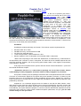
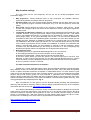
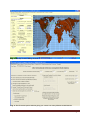
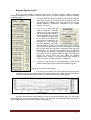
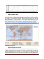
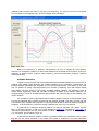
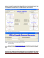
Proplab- Pro 3 – Part 1
A review by ON5AU
At the end of previous year 2007, I
had a look on the internet site of STD (Solar
Terrestrial Dispatch) and I was happily
surprised to find the announcement of their
latest release, Proplab-Pro Version 3,
available from December, 19 - 2007. This
was the promised “Upgrade” I was expected
for many years. In the past I often used
Problab-Pro 2 to illustrate and make
propagation properties visual in my monthly
Propagation column at antenneX. This
software packet was not only a program for
classical propagation predictions, such as
MUF, FOT and Reliability, but in special also
a program to analyze the propagation
properties of high frequency signals in the
ionosphere. This older Version 2 from about 1994 is a DOS related program and has some options not
too user friendly, but nevertheless gave reliable results. At the manual of Proplab-Pro 2 was
mentioned that these less user-friendly options should be resolved in a future Version 3. The time has
come to try out and study the newest release.
Installation
Installing the software was easy and smooth. The minimum system requirements are:
ƒ
ƒ
ƒ
ƒ
ƒ
Windows 2000, XP or Vista
256 MB of memory; recommended 512 MB
2.5 GB of free hard-disk space.
1 GHz microprocessor; recommended a 2+ GHz
Monitor capable of 1024 X 768 pixels; recommended 1680 X 1050 pixels.
I did the test computing for this review with Windows XP, 512 MB memory, 2 GHz Pentium 4
microprocessor and a monitor of 1024 X 768 pixels. For almost all of the available options this was
more than sufficient. However, the 3D ray-tracing option better needs a much higher microprocessor
clock frequency, see later.
A 60-page manual explains all the options and has several colorful illustrations. I quote from
the manual Introduction chapter:
“Problab-Pro Version 3 is a state-of-the-art package not for the faint of heart. A basic
understanding of radio propagation and terms related to radio propagation is presumed.”
This quote is certainly true; the package is therefore also accompanied with the user’s manual
of Version 2--not because it applies in any specific way to the operation of Version 3, (it does not), but
because it has a very nice introduction to radio propagation and ray theory. Reading my columns or
books should also be of great help to have insight into propagation and ionospheric properties, both
published by antenneX.
Proplab-Pro 3 is a Windows program and a lot easier to use than the DOS Version 2 was.
With simple mouse clicks the option windows pop-up and input parameters are easily chosen with
checkboxes, radio buttons and simple input fields. At first startup the program asks you to fill in your
email address. This option allows the program to connect to servers and fulfill the requirements for the
anonymous FTP protocol to collect certain needed ionospheric parameters, and yes, you can work
with the today’s on the spot values.
antenneX Issue No. 131 – March 2008
Page 1 Map location settings
The map option will be used frequently and let you set up several propagation circuit
parameters, Fig. 1.
ƒ
ƒ
ƒ
ƒ
ƒ
Map projections. Thirteen different kinds of map projections are available: Mercator,
spherical hemisphere and oblique Azimuth projections.
Short/long Path. This is the classical toggle selection between the two paths. Here one note:
the 3D ray-tracing engine is limited to short-path only or 20 000 km (half-way around the
globe)
Gray angle. Allows defining the width of the grayzone in degrees, (after sunset – ahead
sunrise, use a negative value, this means the sun below the horizon). One degree equals four
minutes in time.
Transmitter and Receiver Locations. The same classical methods as with Proplab-Pro 2 are
available. However, using the grid-location method, popular amongst the VHF – UHF bands
users is not available with Version 3. Perhaps this can be added in a future update to make
these people happy. A truly great advantage with Version 3 is the enormous database of
worldwide locations with their latitude/longitude coordinates and even their altitude (for the
altitude see later). Speaking of databases, Proplab-Pro 3 is equipped with one of the largest
city databases in the world, nearly 600 000 KB. You can easily and quickly look up any of the
over 5 million city and place names included in the database. A minimum of 3 characters and
waiting 3 seconds after typing your last character is enough to find the location(s). Simply
choose the city that matches what you are looking for and click on it. The corresponding city
latitude and longitude will then be displayed into the appropriated input boxes.
Miscellaneous items.
1- Centering the map on a particular latitude/longitude to your convenience.
2- The bearing and distance for the communication circuit is displayed.
3- Buttons for Redraw Map – display Great-Circle Path and Clear Patch.
4- Set Time mode. Where you have the options: Use Current Real-Time or Set UTC Time
Manually. In case of use current real-time you can define the Map Refresh Interval in minutes
and a countdown counter is displaying how many minutes/seconds left for the map refresh.
5- The sun position is shown on the map.
The 2007 International Reference Ionosphere
Proplab-Pro 3 comes integrated with the 2007 IRI (International Reference Ionosphere) data.
Many different versions of the IRI were released throughout the years. This is the latest and greatest
version of data to describe the Earth’s ionosphere in mathematical terms. For those without a good
grasp, this is truly significant since IRI 2007 is without question, one of the most elaborate and useful
versions that the IRI working group has ever produced. It generates more accurate ionospheric
electron density profiles than ever before and gives Proplab the ability to ray-trace through even more
realistic simulations of the behavior of the Earth’s ionosphere. The end result is greater accuracy, even
during geomagnetically disturbed periods, Fig. 2.
New in Proplab-Pro 3 is the option to use the D-Region Model permitting SW (Stratospheric
Warming) and WA (Winter Anomaly). Data for these D-Region properties and many other ionospheric
informative data can be found at: http://www.swpc.noaa.gov.
An in-depth understanding of what the various checkboxes enables or disables is beyond the
need to know, is what the manual says. They simply turn on or off various models used by the IRI to
calculate ionospheric properties that Proplab-Pro 3 uses. The manual mentions having an Internet
search for “Ionospheric IRI”. I did some searching and the following links might be of help for a start.
Perhaps this is a challenge for a future issue to dig a bit deeper into these matters.
http://modelweb.gsfc.nasa.gov/ionos/iri.html
http://www.ted.isas.jaxa.jp/IRI_News/
antenneX Issue No. 131 – March 2008
Page 2 Fig. 1. The Map location settings window
Fig. 2. The IRI model Options window giving you control over many IRI2007 model features.
antenneX Issue No. 131 – March 2008
Page 3 Electron Density Profile
Once you have defined a communication circuit, Proplab computes several ionospheric
properties, displayed by the Electron Density Profile option. This option displays a window consisting
of individual parts.
ƒ The main part of the Electron Density Profile window displays a
world map showing the circuit path and its distance, and the
day-grayline-night shading. This map serves also for giving
specific details of ionospheric properties of any chosen
location, see below.
ƒ
At the left a table with the
various ionospheric computed
values at the path mid-point,
Fig. 3a. Unique with Proplab 3
is the possibility of finding out
the ionospheric property values
at any point of the world map.
This option is enabled by unchecking the Path Mid-Point
box, see illustration at the right
and thereafter by clicking at any point at the map. Doing so
along the circuit path gives you all the information you would
like to know about the ionospheric properties along that path.
Furthermore, you can find out the altitudes at any location on
the Earth with this feature. This altitude is simply displayed at
the bottom of the Ionospheric Statistics table in the Receiver
Height box. Simply point and click. Note: the altitudes
displayed are in meters. To convert meters to feet, multiply by
3.281 and meters to miles, multiply by 0.00062137.
ƒ
At the top of the window is a chart showing a profile of the
plasma frequencies along the defined circuit path, Fig. 3b.
Fig. 3a. The numerical values table.
ƒ Un-checking the Plasma Freq. Along Path checkbox shows the
vertical electron density profile chart over the path mid-point if the Path mid-point checkbox is
checked. Otherwise the density profile of a chosen location on the map, Fig. 3c.
Fig. 3b. The circuit plasma frequencies chart.
For both, the transverse plasma frequency chart or the electron density chart, you can set the
height range and you have the possibility to zoom in or zoom out. This interesting zooming facility is
also available at many other map and charts with Proplab 3.
antenneX Issue No. 131 – March 2008
Page 4 Fig. 3c. The vertical electron density profile chart.
Global Ionospheric Maps
Proplab-Pro 3 is equipped with a complete suite of ionospheric maps, Fig. 4. You can plot
about anything, such as Maximum Useable Frequencies, ionospheric layers critical frequencies, the
layers height maximum, magnetic field parameters, electron gyro frequencies, etc. New is compared
with Proplab 2: D-layer parameters; Ionospheric Valley Top height; Ionospheric Valley Thickness;
Spreaf-F Probabilities in %; X-Ray Absorption for a given frequency and a ray-traced MUF or FOT.
These additions are of great help to study the ionospheric behavior and the propagation
characteristics in greater detail and more profoundly. Also new is the option Map Transparency, an
attractive feature of Proplab 3 to make the underlying map more or less prominent on the screen.
Fig.4. Global Ionospheric Map
Maximum Useable Frequencies
Compared to Proplab 2, the Version 3 has two additions with the Hourly MUF Graphs option: a
ray-traced FOT and the elevation angle required for a signal at the MUF to reach the destination.
Proplap 3 computes two kind of FOT, the Normal FOT, which is computed as simply 85% of the MUF,
which differ substantially from the ray-traced FOT. The ray-traced FOT is defined as the highest
frequency that permits 85% of the signal to be refracted back to Earth. Why is this information useful?
Because unlike the traditional FOT, this ray-traced definition of the FOT guaranties that 85% of your
antenneX Issue No. 131 – March 2008
Page 5 radiated power will reach the Earth on the given FOT frequency. The same is not true for the Normal
FOT computed in the traditional way, as the plot Fig. 5 clearly illustrates.
Fig.5. MUF chart.
Note: FOT (Frequency of Optimum Transmission): the FOT is usually the most effective
frequency for ionospheric reflection of radio waves between two specified points on Earth. Synonyms:
frequency of optimum traffic, optimum traffic frequency, optimum transmission frequency, optimum
working frequency.
Antenna Selection
Proplab 3 comes pre-built with several standard antenna radiation patterns that can be used to
produce more realistic signal analyses. The radiation patterns are not completely 3-dimensional; the
elevation/azimuth gain tables are simplified to a two and a half dimension. The reason for not using
true 3-D patterns is simply computing speed (not to mention complexity), even with today’s fastest
home-based computer systems. Using partly simplified radiation patterns, the software is able to
render results significantly faster and yet retain a majority of realism in the radiation patterns. The
simplified pattern means an elevation/azimuth gain slide with the maximum gain at that heading of the
chosen antenna.
It is possible to create or generate antenna radiation patterns yourself, not with Proplab 3 itself
but with an additional utility program included with the package, Fig. 6b. This utility converts 2-D and
3-D antenna types useable with VOACAP in conjunction with HFANT to antenna patterns useable for
Proplab 3. In the Proplab-Pro 3 manual is clearly explained how to do such conversions.
A great help for creating the antennas patterns you need to represent your “station antenna
farm” is the extra collection of 3D type-13 files available at antenneX, compiled by L. B. Cebik: 16
collections representing more then 1700 antenna models. Yagi's, quads, various doublets, inverted
V´s, monopoles, ground planes, loops, etc
At the antenna selection window screen it is possible to define the Transmitter Power in watt,
Fig. 6a. It is not clearly explained in the manual if this power is supposed to be at the transmitter
antenneX Issue No. 131 – March 2008
Page 6 output or at the feedpoint of the antenna itself. I suppose the latter because feedline losses can
substantially change from station to station and feedline type and length. When using fixed azimuth
directional antennas it is possible to change the azimuthal bearing to its real-beaming direction. With
rotatable antennas both TX/RX antennas are pointed toward each other automatically.
Fig.6a. The antenna Selection option screen.
Fig.6b. The utility program ITS to Proplab Antenna Converter.
Discussion Group
There is a discussion group established so that owners of Proplab-Pro 3 can exchange ideas
and findings; just navigate to http://www.spacew.com/forum and click on the “Software Discussion”
section, followed by the Proplab-Pro link. An easier way should be an inherent tab-link in Proplab-Pro
itself.
Primary Comments and findings
In the introductory chapter of the manual the authors the write: “Many of the features in
Version 3 are not available in Version 2, and there may even be a few things that were present
in Version 2 that are not present in Version 3. If anyone can spot a feature that is missing from
antenneX Issue No. 131 – March 2008
Page 7 this latest version, by all means let us know. We would love nothing more than to debug
something else!”
I spotted some and mailed Cary about it. Cary answered that most were planned and will be
included in a next build update.
ƒ
ƒ
ƒ
ƒ
ƒ
ƒ
ƒ
All maps, charts or plots can be printed by one mouse click. Version 2 has the additional
possibility to Copy them as a gif file.
No option to define a Sporadic-E layer.
No Auroral zone border lines projection on the maps.
The magnetic disturbance Ap-index is not possible to configure manually.
No option to define Polarcap absorption
No option to define X-ray flare type occurrence.
Location input of TX / RX not possible via Maidenhead grid square locator input.
I also made some suggestions and also these will be taken into account in a next release.
ƒ
ƒ
ƒ
When you hover the cursor above an input field, checkbox, etc, a legend is displayed about
the hovered item. You can disable this option at the Other Options screen. But the time that
the legend is displayed is too short to read properly. So, I proposed to lengthen the display
time or to keep it displayed as long as the mouse cursor hovers the item on the screen.
As mentioned above is a user’s discussion group internet page created. The proposal is to put
a direct clickable link to the user’s group discussion page from Proplab-Pro 3 directly and not
via an additional step, the Windows Internet Explorer.
I proposed also to put a direct Tab from within Proplab 3 to start the utility program ITSconvert. Would be much handier.
The manual is good explaining the features of Proplab 3 and well documented with colorful
illustrations. Those who have experience with Proplab Version 2 will encounter no problems to use the
new Version 3, contrary; it is now less cumbersome and much handier to define all the necessary
input parameters. For those not familiar with the older Version 2 is the accompanied manual of this
version a great help to understand ionospheric behavior and properties and some explanation about
the use of the ray-tracing engine and different analysis.
Proplab-Pro Version 3 can be ordered and downloaded via Internet or on CD-ROM at the STD
website. Delivered via Internet, the package costs $240 USD. Perhaps this sound rather high at first
glance. But taking into account the huge man-hours to program and to create the unique worldwide
locations and topographical databases plus the much better accuracy of the ray-tracing models makes
it more than worth its price. As mentioned at the start, I was looking toward a new release of ProplabPro since years and I am very happy it is finally available.
More to come
One option is not discussed yet, the ray-tracing of radio signals. This option is the one that
Proplab-Pro distinguishes the most from any other propagation prediction program. Proplab-Pro 2 was
considered by many around the world as the most powerful radio propagation diagnostic tool in the
world in spite of some drawbacks, which are solved in Proplab-Pro 3. This ray-tracing is rather
complex in particular for the novice user but more than worth learning how to do and interpret it by
analysis with knowledge. This will be entirely the Part 2 subject. So, stay tuned. -30-
Click for Author's Biography
antenneX Online Issue No. 131 — March 2008
Send mail to [email protected] with questions or comments.
Copyright © 1988-2008 All rights reserved worldwide - antenneX©
antenneX Issue No. 131 – March 2008
Page 8