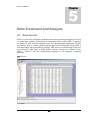
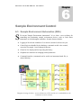
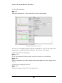
1
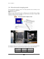
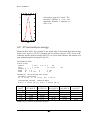
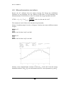
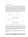
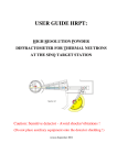
PAUL SCHERRER INSTITUTE Laboratory for Neutron Scattering Rita II Manual Version 1.3 LABORATORY FOR NEUTRON SCATTERING Rita II Manual Christof Niedermayer and Niels Christensen Laboratory for Neutron Scattering Paul Scherrer Institut CH 5232 Villigen PSI Phone +41 56 310 2086 • Fax +41 56 310 2989 [email protected] [email protected] Table of Contents The Instrument 2 3.3 1.1 Beamline and Guide 3 to point focusing mode 1.2 Monochromator 4 3.4 1.3 Beam Monitor 5 imaging mode 25 1.4 Sample Table 6 RITA II Alignment 26 1.5 Motorized slits 7 4.1 Monochromator 26 1.6 Filters 7 4.2 2T and neutron energy 27 1.7 Analyzer 8 4.3 Monochromator 1.7.1 The analyzer tank 8 curvature 28 1.7.2 The nine-bladed analyzer 8 4.4 29 1.8 Position 9 Data Treatment Analysis Sensitive Detector Short User Manual 11 2.1 Introduction to SICS 2.1.1 RITA-2 Configuration 2.2 Starting SICS 2.2.1 six 2.3 Drive, 2.4. OMA calibration and 32 11 5.2 Data Storage 33 12 5.3 Data Analysis 33 13 5.3.1 Data Conversion 33 5.3.2 Matlab Routines 33 UB Matrix and Crystal 15 2.4.1 Example Session 16 2.4.2 Out Of Plane Operation 18 2.5. Scan command 2.6. Other Commands and 19 Procedures Monochromatic 32 14 Alignment 20 Sample Control 6.1. Environment 35 Sample Environment Automation (SEA) 35 The Oxford 15T magnet MA15 37 7.1 Regulations and Specifications 37 38 7.2 Installing MA15 2.6.1 Simulation Mode 20 7.3 Change 2.6.2 Batch files 20 Omega 2.6.3 Counter Box Threshold 21 Stick 2.6.4 Monochromator Curvature 22 2.6.5 Scattering Sense 22 Index Rita Modes 3.1 23 Two axis and three axis modes 23 3.2 23 Flat mode 24 Data Format and Modify device parameters point 5.1 13 Check Monochromatic Motor to / from on Sample 42 43 T H E 1 Chapter I N S T R U M E N T The Instrument R ita II is a triple axis spectrometer for cold neutrons at the Swiss Spallation Neutron Source SINQ at the Paul Scherrer Institute in Villgen, Switzerland. The instrument is being operated in a joint venture between the Paul Scherrer Institute and the RISOE National Laboratory, Denmark. RITA II is based upon the conventional triple-axis idea, optimized in several ways. Its main components are: Supermirror coating (m=2) in the neutron beam guide A vertically focusing monochromator Motorized slits Be and BeO filters with built-in collimators A flexible 9-bladed analyzer A position-sensitive detector (PSD) A vertically focusing monochromator The multi-bladed analyzer combined with the PSD provide flexibility for measurement and opportunities for getting additional efficiency. 2 T H E I N S T R U M E N T 1.1 Beamline and Guide The neutrons from the Swiss Intense Neutron Source SINQ leave a cold source end enter the guide system RNR13. The primary super mirror (m=2) beam guide is 20 m long and has a curvature radius of 2408 m. The guide cross section is 12 x 3 cm2. Neutron fluxes were determined by gold foil activation and are given in the figure below. The SINQ instrument hall at PSI showing the neutron beam line from the source through the guides to the spectrometers. RITA2 is located at the position of the former Drüchal triple axis spectrometer. The flux measured by gold foil activation is also shown. Intensity versus wavelength given as monitor counts per second. 3 T H E I N S T R U M E N T 1.2 Monochromator The RITA II monochromator consists of 5 (vertical) x 3 (horizontal) PG (002) vertically focusing crystals of size 5 cm width * 2.5 cm height. The mosaicity is 40' in both directions. The curvature of the monochromator is controlled by the motor CUM, which turns the blades. The turning of the blades is given by CUM (in arbitrary units) for blade 2 and 4, twice that amount for blade 1 and 5. The optimal curvature depends on the spectrometer energy (see chapter 2). The proper curvature is automatically set by most scan files. The translations of the monochromator are TUM (in arbitrary units) and TLM (in arbitrary units). The monochromator goniometer is GM. The monochromator is rotated by the motor OMM (or A1, all angles in units of degrees). The corresponding scattering angle is 2TM (or A2). There is an encoder on this angle. The monochromator d – spacing is set by the variable DM (3.354 Å for PG 002). 4 T H E I N S T R U M E N T 1.3 Beam Monitor RITA II is equipped with a 3He beam monitor with an opening of 80*40 mm2. This is normally located on a holder on the first motorized slit, right at the exit of the monochromator shielding. The monitor counts are stored in the SICS variable MON, and the corresponding rate meters are called RmS, RmM and RmF for slow, medium and fast response times, respectively. The units are counts/sec. Normal monitor count rates are given in the following table. Configuration Seconds per 1000 Monitor Measuring time for 10000 Monitor. 5 T H E I N S T R U M E N T 1.4 Sample Table The centre of the sample table is placed 1.406 m from the monochromator axis. This table is designed to hold one of Risøs cryostats or magnets, see the page about the auxiliary equipment. Alternatively, an open-air sample holder, a monitor holder, or an Eulerian cradle may be put on the table. The maximum dimensions for cryostats on the sample table are approximately given by the Risø 9 T magnet: height 150 cm, diameter 44 cm, weight 450 kg. The sample table is shown in Fig. 1. Figure 1: Pictures of the sample table at the RITA II spectrometer. The sample table is rotated by the motor OM (A3); the corresponding 2 angle is called 2T (A4). The maximum movement of 2T is limited by the neutron guide and hence depends on the value of 2TM as given in the following table: Energy (meV) 3.7 5 13.68 14.7 2TM 89.0 74.16 42.76 41.18 Maximum in 2T -118 -115 -90 -81 Above the turning plate, there are two translations motors (TU and TL, in units of mm), and above these are two goniometers, GU and GL (measured in degrees). The height from the top of the sample table to the beam centre is 110 mm. Cryostats, magnets, and open-air sample holders are constructed so that the height from the sample mount to the beam is 57 mm. 6 T H E I N S T R U M E N T 1.5 Motorized slits There are four optical benches: Before and after the sample and inside the analyzer tank before and after analyzer. Each can hold a motorized slit. The slits are made from four 10 mm thick BN plates which attenuate the beam by more than 4 orders of magnitude. Each of the four plates has a motor connected. For the monochromator slit the motor names are MSL, MSR, MSB and MST (the third letter denotes left, right, bottom, and top, respectively). The slits after the sample are SSL, SSR, SSB and SST. The analyzer slit motors are named ASL, ASR, ASB and AST and the detector slit motors are DSL, DSR, DSB and DST. All eight motor values are in units of mm. Neutron monitor and motorized slit after the monochromator. 1.6 Filters RITA II has two radially collimating filters - a Be and a BeO filter. The filters are meant to be placed right before the analyzer tank, to filter out elastically scattered neutrons in an inelastic experiment. The filters a placed on a special holder and can easily be drawn in or out of the neutron beam. The filters are cooled with liquid nitrogen and have a hold time of 36 h when pumped out well. The filters have to be aligned. The rotation angles are 4 degrees for the BeO filter (marked on the filter support) and 0 degrees for the Be filter. Pictures of the BeO filter and the filter support. The filter can easily be pushed into or out of the beam. 7 T H E I N S T R U M E N T 1.7 Analyzer 1.7.1 The analyzer tank The tank housing the whole analyzer/detector system is shown in fig. 1. The outer walls are made from a mixture of polyethylene and boric acid, and the inside of the stainless steel tank is covered with 5 mm boron-containing plastic. This construction minimizes the neutron background, as most of the fast neutrons are thermalized by hydrogen in the thick walls, while thermal and cold neutrons are absorbed by the boron nuclei. The walls have an Al opening where neutrons scattered at the sample enter the tank. Here a collimator may be inserted. Figure 1: Sketch of the RITA2 analyzer tank. For monitoring the equipment inside the tank, a small video camera is placed inside the tank and the output is displayed on a video monitor on the control platform. Entrance to the tank is easy accessible by opening the tank doors, see fig. 2. An optional front shielding is shown on the figure too. Further additional shielding for the inside of the tank is available. 1.7.2 The nine-bladed analyzer The nine-bladed PG analyzer (at the moment only 7 blades are installed) of the RITA II spectrometer is shown in fig. 3. The blades have the dimensions 24*150 mm2 and are mounted on vertical axes, each with its own motor. The nine motors are named CA1 8 T H E I N S T R U M E N T through CA9 (where the angle is given in degrees), and they are in turn mounted on an analyzer module with a distance of 25 mm between them. The analyzer axis is located 120.7 cm from the center of the sample table. The analyzer module is also able to rotate around a vertical axis; the corresponding motor is called OMM (A5 when working in one of the standard triple axis modes). All blades of the analyzer may be set to the same angle by the command PARK a, where a is the setting angle, i.e. a flat analyzer is obtained by typing PARK 0. As for the monochromator, the d-spacing of the reflection at the analyzer must be stated, this is done by setting the variable DA (3.354 Å for PG 002). 1.8 Position Sensitive Detector For counting the neutrons, RITA II uses a 30x50 cm2 position-sensitive detector (PSD), which bins the neutron counts into 128 x 128 pixels, see fig. 1. The distance from the analyzer axis to the detector face is variable and the maximum value depends on the position of the analyzer. The detector is able to swing around in the tank to one side only, see fig. 2. The corresponding motor name is 2TA (A6). 9 T H E I N S T R U M E N T 10 S H O R T U S E R 2 Chapter M A N U A L Short User Manual I n this chapter we will give a brief introduction into the SINQ Instrument Control System SICS and the most relevant commands needed to control the instrument during an experiment. Convention for type-setting in this manual: <device> stands for all drivable variables (motors, fields, temperatures, etc.) <value> stands for a required variable entry [<value>] stands for an optional variable entry entrances marked with SICS are meant to be written in the command line in the SicsClient entrances marked with term are meant to be written on the console (e. g. in a xterm) 2.1 Introduction to SICS SICS (SINQ Instrument Control System) is a client-server system that controls all neutron spectrometers of SINQ. There is a magic server program running on the instrument computer which does all the work. The user interacts with SICS only with client applications which communicate with the server through the network. Most instrument hardware (motor controllers, counter boxes etc.) is connected to the system through RS-232 serial connections. These RS-232 ports are connected to a terminal server which is accessed through another server program, the SerPortServer program, which is also running on the instrument computer. The SICS server communicates with the terminal server and other devices through the network. The program was written by Mark Koennecke and a detailed description can be found in the SICS manual. 11 S H O R T U S E R M A N U A L FIGURE 1.1 Hardware Setup at SINQ 2.1.1 RITA-2 Configuration pc4345, rita2 Instrument computer, running Linux lnsgpib01 TCP/IP-GPIB bridge psts216 Terminal server. All ports configured 9600,8,1,no parity, no flow control, if not stated otherwise. Ports: port 2 EL734 motor controller port 3 Risø temperature log port 7 Lakeshore temperature controller 12 S H O R T U S E R M A N U A L 2.2 Starting SICS 1. Check, if the SICServer is running: term ps -A | grep SICS should report at least one line ending with term…… SICServer rita2.tcl. If not, type term startsics For this you’ll have to be user rita2 on the computer rita2.psi.ch. 2. Start the SicsClient: term sics& a new window will open. 3. Activate SICS via the pull down menu in the SicsClient: Connect / RITA2 and 4. Authorize: Enter User Name and Password standard user name and password are rita2user and 03lns1 5. Start the status-window: term rita2status & 6. Activate the status-window via the pull down menu: Connect / RITA2 7. An online plot of the PSD can be obtained by term sansstatus & 8. Activate the status-window via the pull down menu: Connect / RITA2 2.2.1 six six is an alternative to the standard Java SICS commandline client. Why an alternative SICS client? It is much faster It does not need the X window system It connects automatically to the instrument if you are logged into the instrument computer 13 S H O R T U S E R M A N U A L It has the full functionality of the standard commandline client, but no graphical interface. This means you can not (and have not to) use the mouse there are no colors to distinguish commands, responses and errors instead of clicking on the interrupt button, you have to enter ”stop” the history is only accessible with the arrow keys 2.3 Drive, Check and Modify device parameters The current value of a device is reported by just typing its name: SICS <device> There are hardware and software limits for all motors. These can be checked for an individual motor by typing SICS <device> list To change the software limits type: SICS <device> softlowerlim <value>, e.g. SICS ca5 softlowerlim -200 SICS <device> softupperlim <value> For PSI motors and encoded RISOE motors (2t and 2ta) repositioning should be done by the command sp, which changes the softzero value. SICS sp <device> <value>sp, e.g. SICS sp omm 37.07 Repositioning of unencoded RISOE motors can be done by the command SICS<device> putpos <value>, e.g. SICS oma putpos 74.17 (This is however at the present state of development not working properly for all motors) The hardware limits can not be changed! Drive a device to a value: SICS dr[ive] <device> <value> Drive several devices at the same time: SICS dr[ive] <device1> <value1> <device2> <value2> [etc.] 14 S H O R T U S E R M A N U A L 2.4. UB Matrix and Crystal Alignment SICS cell a b c alpha beta gamma set unit cell constants. If b or c are omitted, the same value as for a is used, if angles are omitted, they are set to 90 degress. Without arguments, the cell constants are listed. SICS ref qh qk ql a3 a4 sgl sgu Ei Ef Make an entry in the list of peaks. For angles and k-values not given, the current motor positions are used. If the given qhkl triple already exists, its list entry is overwritten. If not, a new entry is made. The peak number and the peak data are returned. SICS addauxref qh qk ql Add an auxiliary reflection to the list of reflections. A4 is calculated from the cell constants, the current ei and ef values are used. A3 is left alone or is calculated to have the right angular difference to the previous reflection. Using auxiliary reflections is a help during setup of the instrument or in powder mode. The sequence: SICS ref clear SICS cell aa bb cc alpha beta gamma SICS addauxref ax ay az SICS addauxref bx by bz SICS makeub 1 2 with ax, ay, az being the first plane vector and bx, by, bz being the second plane vectors creates a UB matrix which allows to drive QE positions and qm. But be aware that a3, sgu and sgl values are still invalid. SICS ref clear peak Remove a peak. SICS ref clear all Remove all peaks. SICS ref List all peaks. SICS makeub peak1 peak2 Calculate, activate and print out the UB matrix, as well as the peak list with qhkl values calculated back. Peak 1 is used as the main peak, i.e. driving to the angles given for this peak will correspond to a QHKL which may only differ by a scalar factor of about one, if the cell constants are not correct. peak2 is used only for determining the scattering plane. SICS makeubfromcell Calculate and activate a UB which has been derived from the cell constants alone. This is useful to get a4 when no reflection has yet been found to calculate a proper UB. 15 S H O R T U S E R M A N U A L SICS makeauxub qh qk ql Calculate a UB matrix from the first reflection and an auxiliary second reflection specified through the miller indices qh , qk, ql. The auxiliary reflection will have the same angles as the first reflection, except a3 and a4 will be adjusted to match the requirements from the crystals geometry. SICS listub List the UB matrix, the cell constants and all stored reflections. 2.4.1 Example Session First enter the cell parameters SICS cell 2.88 2.88 2.88 90 90 90 Define the scattering plane SICS addauxref 2 0 0 SICS addauxref 0 2 0 SICS makeub 1 2 Calculate and activate a UB which has been derived from the cell constants alone. Drive the instrument to the calculated A4 position. SICS dr a4 position Find the peak 2 0 0 and optimize it. Once you are at the maximum: SICS ref 2 0 0 Peak QH QK QL A4 A3 SGL SGU 1 2.00 0.00 0.00 65.31 -87.21 1.25 -5.22 Make an axiliary UB and drive to the theoretical position for 0 4 4 SICS dr qh 0 4 4 Find the 0 4 4 reflection and optimize. Once you are at its maximum: SICS ref 0 4 4 Peak QH QK QL A4 A3 SGL SGU 1 0.00 4.00 4.00 65.31 -87.21 1.25 -5.22 Show the complete peak list: SICS ref Peak QH QK QL A4 A3 SGL SGU 1 2.00 0.00 0.00 65.31 -87.21 1.25 -5.22 2 0.00 4.00 4.00 99.45 20.39 4.25 -1.22 16 S H O R T U S E R M A N U A L Calculate the UB matrix, with 2 0 0 as primary peak and 0 4 4 as secondary peak. SICS makeub 1 2 UB 2.456 0.530 -0.200 -0.530 2.456 -0.090 0.200 0.090 2.456 Peak QH QK QL A4 A3 SGL SGU QH QK QL 1 A 2.00 0.00 0.00 65.31 -87.21 1.25 -5.22 2.03 0.00 0.00 2 B 0.00 4.00 4.00 99.45 20.39 4.25 -1.22 0.02 3.95 4.03 The last 3 columns above show the Q values calculated back from the angles. Drive to the 2 0 0 peak SICS dr qh 2 0 0 SICS pr A4 A3 SGL SGU A4 = 64.218 A3 = -87.515 SGL = 2.258 SGU = -3.217 The value of A4 has changed, because the cell constants do not match the values given for the first peak. The value of A3 has changed by the same reason, and in addition, because the the plane given by 2 0 0 and 0 4 4 is now tilted back into in the scattering plane. For the latter reason SGU and SGL have changed also. SICS DR QH 3 3 3 SICS PR A4 A3 SGL SGU A4 = 82.516 A3 = -31.215 SGL = 2.258 SGU = -3.217 Note that the values for SGU and SGU have not changed. The will not change as long as we stay in the scattering plane (no drives to Q3) and as long as the UB matrix has not changhed. SICS REF 3 3 3 Peak QH QK QL A4 A3 SGL SGU 3 3.00 3.00 3.00 82.32 -31.25 2.26 -3.22 SICS MAKEUB C B UB 2.456 0.530 -0.200 -0.530 2.456 -0.090 0.200 0.090 2.456 Peak QH QK QL A4 A3 SGL SGU QH QK QL 1 2.00 0.00 0.00 65.31 -87.21 1.25 -5.22 2.03 0.00 0.00 2 B 0.00 4.00 4.00 99.45 20.39 4.25 -1.22 0.02 3.95 4.03 17 S H O R T U S E R M A N U A L 3 A 3.00 3.00 3.00 82.32 -31.25 2.26 -3.22 3.00 3.00 3.00 We have calculated a new UB matrix, based on the peak 3 3 3 as primary and the 0 4 4 as secondary peak. The UB matrix has not changed, as we were already exactly at 3 3 3. 2.4.2 Out Of Plane Operation This formalism allows to drive out of the scattering plane using the tilt motors of the sample stage. Some cryostats cannot stand this. Therefore driving out of plane can be switched off and on. SICS TASUB OUTOFPLANE 1 This command switches out of plane operation on. SICS TASUB OUTOFPLANE 0 This command switches out of plane operation off. SICS TASUB OUTOFPLANE lists the current value of the out of plane variable 18 S H O R T U S E R M A N U A L 2.5. Scan command The scan syntax is like on TASMAD. The general scan command is SICS sc[an] <device> <center> <step> <np> <preset> with the arguments : <device> any driveable variable, and <center> its center value <step> any step (d immediately followed by the variable name) <np> followed by the number of points <preset> followed by the monitor mn or time ti preset value The presence of 4 argument parts is mandatory, but the order of the parts is not relevant. For every step variable, the corresponding center value must be given. If no step is given for a center variable, a step 0 is used. Special cases are the variables QH and Q3 , and their corresponding steps DQH and DQ3 which have 4 or 3 values. Examples: SICS SC A3 40 DA3 0.1 NP 41 MN 1000 orders a scan of A3 around 40 degrees with 20 steps to either side with a step width 0.1 and 1000 counts in the monitor. Alternatively, the preset value time gives the counting time in seconds. SICS sc a3 40 da3 0.1 np 41 ti 1 Energy scan (the following two beeing equivalent)) SICS SC QH 1 0 0 0 DQH 0 0 0 0.01 NP 5 MN 1000 SICS SC QH 1 0 0 EN 0 DEN 0.01 NP 5 MN 1000 q scan (the following two beeing equivalent)) SICS SC QH 1 0 0 0 DQH 0 0.01 0 0 NP 5 MN 1000 SICS SC QH 1 0 0 0 DQH 0 0.01 0 NP 5 MN 1000 The scan uses the value of <device> and the number of counts window 5 as plotting variables in rita2status. One can also scan multiple motors. For example a - 2 scan is performed by the following command: SICS sc a3 40.2 da3 0.1 a4 73.5 da4 0.2 np 41 mn 1000 19 S H O R T U S E R M A N U A L 2.6. Other Commands and Procedures 2.6.1 Simulation Mode For testing batch files or in order to check the movement of the instrument it may be helpful to run SICS in simulation mode. You must then connect to a special simulation SICS server. Open a new sics client and connect to RITA-2-SIM. term sics & In the simulation server, everything is like in the actual SICS server, except that no hardware is moved, no counts collected and no data file written. There is one specialty, however. The command: SICS sync synchronizes the parameters and limits in the simulation server with those in the instrument. 2.6.2 Batch files To see the batch file path: SICS exe batchpath To change the batch file path: SICS exe batchpath newpath, e.g. SICS exe batchpath /home/rita2/batch To write a batch file: Produce a text file with a text editor of your choice (emacs, kate etc) term kate test01.job &" Write the commands directly into the text file, as you would have done at the SICS client. Save the file in the batch directory defined above To execute the text file type SICS do test01.job The batch file can not be changed once it is executed. A workaround this limitation is to call another batch file at the end of the file. 20 S H O R T U S E R M A N U A L Example of a batchfile dr ef 5 ritamode monoim dr tt 10 wait 600 dr mf=5 title (H,L)scan, E=0.7meV, H=5T sc qh -0.5 0 0.98 0.7 dqh 0.005 0 0.0072 0 np 41 mn 200000 dr mf=0 title (H,L)scan, E=0.7meV, H=0T sc qh -0.5 0 0.98 0.7 dqh 0.005 0 0.0072 0 np 41 mn 1e6 title energy scan at (1 0 1), H=0T sc qh 1 0 1 1.5 dqh 0 0 0 0.1 np 41 mn 2e5 do nextjob.job 2.6.3 Counter Box Threshold To prevent collecting background data in case of no beam or a very low beam a threshold value should be set on the PSI counter-box. (In TASCOM this was done by the command CIBO and setting the threshold manually). The PSI counter-box is now accessible from SICS. The following commands are available: SICS el737 getthreshold 1 reads the current threshold SICS el737 setthreshold 1 <value> sets a new threshold. Typical values are 20 to 50. 21 S H O R T U S E R M A N U A L 2.6.4 Monochromator Curvature The curvature of the monochromator is controlled by the motor CUM, which turns the blades. The optimal curvature depends on the spectrometer energy and is given by CUM vb1 vb2 / sin(omm) with vb1 0.307 and vb 2 8.90 (as of April 2007) These values can be changed by the command SICS tasub mono vb1 value SICS tasub mono vb2 value The gain in intensity compared to a flat monochromator is about 2.5, as can be seen from the figure below. 2.6.5 Scattering Sense Most experiments are done in a sm=1, ss=-1 and sa=1 configuration, where +1 means scattering to the left and -1 scattering to the right. Sm and sa can only be +1, only the scattering sende at the sample can be changed by SICS se ss value or SICS tasub ss value 22 R I T A 3 Chapter M O D E S Rita Modes S electing the analyzer mode is an important issue for the RITA II spectrometer. In this chapter we describe the different modes which are available at present for standard operation. 3.1 Two axis and three axis modes The spectrometer can be run both in two - axis and triple – axis mode. There are 2 triple-axis modes: ki and kf. (fixed incoming or fixed final energy). Usually the kf option is used. There is only one 2-axis mode: elastic. To read which mode the spectrometer is in write SICS tasub const To change the mode write for instance SICS tasub const elastic To avoid a shadow from the edge-on analyzer in two axis mode one may like to turn away OMA (to e.g. 90 degrees) and lock it by SICS fix oma 3.2 Flat mode This mode is selected by the command SICS ritamode flat The nine-bladed analyzer is made flat (all cai zero) and oma equal to omm (In standard triple axis notation A5 = A1). 23 R I T A M O D E S 3.3 Monochromatic point to point focusing mode A monochromatic point-to-point focusing mode which produces a reasonable E resolution and a relaxed Q resolution is obtained by SICS ritamode focus This mode focuses the beam on the central part of the PSD. Analyzer configuration in focusing mode. The 7 blades focus the beam on the central part of the PSD. The outer parts of the PSD are covered up by borated polyethylene pieces, which can be screwed to the detector housing. 24 R I T A M O D E S 3.4 Monochromatic imaging mode The monochromatic q dispersive mode is now fully operational and can routinely be used for experiments. It is obtained by SICS ritamode monoim In this mode the different blades scatter on different parts of the PSD and have slightly different q values. In order to minimize cross talk between the blades a flexible radial collimator is installed in front of the PSD. Analyzer configuration in monochromatic q-dispersive mode. The collimator blades can be driven by the two motors lc and rc for the left and right half of the collimator, respectively. Typical values for lc and rc are given in the table below: Ef (meV) 3.7 5.0 lc 77 22 rc 20 0 25 R I T A 4 Chapter M O D E S RITA II Alignment 4.1 Monochromator Insert 40’ collimator into the beam opening of the monochromator shielding. Place a 15 mm slit in front of the monitor, which is mounted on the 600 mm X95 profile. Drive monochromator flat (no curvature) SICS dr cum 0 Drive A2 (2TM) to the desired value (see Table 1) Scan (A1) OMM around its nominal value. In order to do this you have to set the counterbox threshold to zero and scan by time (stable beam required) SICS sc omm current_value domm 0.05 np 21 ti 1 find maximum intensity for OMM, drive there and redefine OMM by 2TM/2. SICS sp OMM 2TM/2. Energy [meV] 3.63575 5.0 8.0 13.68 Wavelength [Å] 4.7434 4.0448 3.1977 2.4453 OMM (Monochromator °) 45.00 37.08 28.47 21.38 2TM (2 Monochromator) 90.00 74.17 56.94 42.76 Tabelle 1: Scattering angles A1 (OMM) and A2 (2TM) for specific energies The monochromator is mounted on a goniometer (motor name GM). Check GM by performing a scan. Before doing so insert a vertical bezel in front of the monitor (vertical opening 30 mm) SICS sc gm current_value dgm 0.1 np 21 mn 1000 26 R I T A M O D E S FWHM=1.139° (GM)=1.0876 Goniometer scan at E=4 meV. The measured FWHM is 1.14° and maximum Intensity is obtained at GM = 1.08 1500 1000 500 0 -1 0 1 2 3 GM 4.2 2T and neutron energy Mount the Risø TAS-6 Al2O3 sample on the sample table. to determine the neutron energy and the zero point of A4 (2T) (Counting rate in auxiliary detector AUX). Insert a 40’ collimator into the analyzer housing. RITA-2 is in 2 axis mode. Measure the intensity of a peak with both negative and positive A4 (2T). Lazy-Input for Al2O3: TITLE AL2O3 CONDIT 2.4571 5.0 75.0 NE CELL 4.76100 12.99100 SPCRGP R -3 C ATOM AL 1 0 0 0.355 ATOM O 1 0.303 0 0.25 120 INTENSITY CALCULATION FOR AL2O3 TRIGONAL STRUCTURE A= 4.76100, C= 12.99100, WL= 2.45710 SCATTERING FACTOR COEFFICIENTS B(Al)= 0.34490 CM-12, B(O)= 0.58030 CM-12 Energy [meV] Intensity 3.63575 5.0 8.0 13.68 2 (012) d=3.4811 Å 84.5 85.89 71.04 54.68 41.13 2 (104) d=2.5513 Å 56.9 104.87 77.61 57.27 2 (006) d=2.1652 Å 143.7 95.20 68.76 Table : Al2O3 reflexes at different energies 27 2 (113) d=2.0861 Å 693.68 100.07 71.76 2 (116) d=1.6017 1176.62 99.52 R I T A M O D E S 4.3 Monochromator curvature Remove the 40’ collimator from the analyzer housing. Die Energie der einfallenden Neutronen ist nun bestimmt, was nun optimiert werden kann, ist die Krümmung des Monochromators CUM. SICS uses a macro to calculate the energy dependnet curvature: CUM A1 A 2 2 d PG 002 E with A1=0.44 und A2=10.87 81.804 The constants A1 and A2 have to be determined experimentally. Mount a Vanadium sample. Set A4 to 90 degrees. Perform cum scans at different neutron energies. SICS dr ef 5 SICS sc cum 26 dcum 1 np 51 mn 1000 SICS dr ef 8 SICS sc cum 26 dcum 1 np 51 mn 1000 Intensity versus monochromator curvature CUM at Ef = 14.68 meV. From the energy dependent maxima CUMmax(Ef) one can determine the SICS - macro parameters A1 and A2. 28 R I T A M O D E S 4.4 OMA calibration It has for some time been a problem that the angle between the analyzer rack and the beam (motor OMA) cannot be properly calibrated. This is due to the flexibility of the analyzer in the capability of turning the analyzer blades. As the blades turn around the same axes as OMA (certainly blade 5), only one of these angles can be calibrated. The analyzer consists of 7 blades numbered 2 to 8 controlled by the motors ca2 to ca8. The point-to-point focusing mode (ritamode focus) was designed to monochromatically focus the beams reflected from the different blades of the analyzer to the same point on the detector. Because of the asymmetry of the analyzer rack relative to the incoming neutron beam and the asymmetry of the detector to the analyzer, the beams from the different blades will actually intersect the detector at slightly different positions. This is seen in figure 1(a) calculated theoretically, assuming 5 meV neutrons and perfect alignment of all angles. The calculated intersection points on the PSD in the point-to-point focusing mode. The beam from the central blade (ca5) is defined to intersect the detector at 0. This corresponds to pixel 64 on the PSD. The exact position of the intersection can be controlled with the motor 2TA. Actually this can be used to calibrate 2TA. In the following it is only the relative position of the intersections, that is important. It is seen in figure 1(a), that the rest of the blades intersect the detector nearly pairwise, in distances increasing with the blade distance from the central blade. Plotting these distances from the central blade as a function of blade number gives a parabola, see figures at the end. If the angle OMA is above or below the perfectly aligned value, the centerof the parabola will be shifted, and the intersection of the beams will not be pairwise, see figure 1(b) and the figures at the end. 29 R I T A M O D E S This section will describe alignment of OMA and the analyzer blades using the point-topoint focusing mode. The energy is set to EF = 5 meV, corresponding to 2TA = 74.17◦. First invoke this mode by ritamode focus, making sure that all the blades are free to move. Place a vanadium or plastic sample on the sample table. Run cascan macro. This will scan each blade one at a time, leaving the others parked at 0. After each scan a pixscanx of the PSD i taken at the most intense position of the blade. This gives the position of the blades reflection on the PSD. The macro gives a table showing the old position, the maximum intensity position and the position on the PSD of each blade. Plot the positions of the blades versus blade number, and connect the points with a parabola. The position of the center of the parabola gives the error in OMA. The figures at the end can be consulted to determine the magnitude of the error. Now move OMA by subtracting OMA and remo to the value it had before. (i.e. if OMA is 74.17◦ and OMA is found as -2◦, set OMA = 76.17 and remo to 74.17.) Move the ca motors according to the movement in OMA. BUT note that the values of the ca motors rise clockwise opposite to all other motors, where the values rise anticlockwise. This means that the ca’s must be compensated in the same (numerical) direction as OMA. If the change in OMA angle is considerable (more than 1−2 ) the blades should be recalibrated with the cascan macro, as the asymmetry means that the blades can not be compensated by exactly the same amount as OMA is moved. 30 R I T A M O D E S Peak position on the PSD for the different blades for a negative OMA (EF = 5 meV). Peak position on the PSD for the different blades for a postive OMA (EF = 5 meV). 31 R I T A 5 Chapter M O D E S Data Treatment and Analysis 5.1 Data Format NeXus is a joint effort of both the synchrotron and neutron scattering community to develop a common data exchange format based on a hierarchical data format (HDF). As physical file format the HDF from the National Center for Supercomputing Applications (NCSA) was choosen. This is a binary, platform independent, self describing data format. HDF is well supported by major data analysis packages. HDF files are accessed through a library of access functions. This library is public domain software. Libraries are available for the ANSI–C, Fortran77 and Java programming languages on all important computing platforms. term hdfview 32 S A M P L E E N V I R O N M E N T C O N T R O L 5.2 Data Storage Under the directory /home/rita2 a directory data/ exists. In data/ you will find some directories according to each year (2006/, 2007/,...). Starting from 2006 onwards within the year directory the data files are grouped in subdirectories for each 1000 data files named 001/, 002/, 003, etc. All data files produced are stored in these directories according to the year and number they were obtained. The data files have the general syntax rita2yearnxxxxxx.hdf with xxxxxx (6 digits) the run number of the file and year the year of production, e.g.: home/rita2/data/2010/001/rita22010n001258.hdf Routinely all new data files are backed up immediately on the machine lnsa15.psi.ch, which is accessible through the AFS file system at PSI. Within UNIX environment one has to get access to the directory root/afs/psi.ch/project/sinqdata/2010/rita2 and then to the desired data subdirectory. From there one can copy files to other disks etc. afs/psi.ch/project/sinqdata/2010/rita2/001/rita22010n001258.hdf 5.3 Data Analysis 5.3.1 Data Conversion You can convert the hdf data into an ASCII file, which you can then import into your favorite data analysis program. term hdf2ascii(`filename`) converts to filename.asc in the current directory 5.3.2 Matlab Routines Log on to the Rita computer term ssh –x rita2@rita2 Ask local contact for password. term cd matlab setup the necessary path info in mypaths. 33 S A M P L E E N V I R O N M E N T C O N T R O L Matlab s=hdf2spec(`filename`,`scanvariable`,flag) e.g. s=hdf2spec(`/afs/psi.ch/project/sinqdata/2010/rita2/001/rita22010n001258.hdf`,`E5`,1) Creates a 1x7 spec1d object. Flag = 0,1 divides (1) or does not (0) divide by monitor Matlab Det_Images(‘filename’) e.g. Det_Images(’/home/rita2/data/2010/001/rita22010n001258.hfd’) Graphical User Interface Matlab qad_view [fs,ps]=fits(s,’gauss’,[1 2.4 0.2 0], [1 1 1 1 ]) Gaussian fit to s with start parameters [1 2.4 0.2 0] (Amplitude, Position, width, Background) 34 S A M P L E E N V I R O N M E N T C O N T R O L 6 Chapter Sample Environment Control 6.1. Sample Environment Automation (SEA) S EA means "Sample Environment Automation". It is a client - server software for controlling and monitoring sample environment devices, such as Lake Shore temperature or Oxford magnet controllers. Its main features include: Logging of all relevant variables at 5 sec interval, stored for at least one year Control logic not handled by the hardware: automatic needle valve control, correction for sample - heat exchanger difference Charts for live display and for inspecting the history Graphical user interface for changing control parameters Command interface (commands can be used in an instrument batch file, or entered directly) Diagram showing the client - server architecture of SEA and how it is embedded into the instrument control software. 35 S A M P L E E N V I R O N M E N T C O N T R O L To start a SEA client enter term sea & on the unix command line, or click on the SEA icon on the linux desktop. The SEA graphical user interface Once the sea user interface appears select the cryostat/device in use, if not already done automatically. (e.g. DISE for the Risoe Displex E, MA15 for the 15 T magnet) In SICS temperatures are changed by: SICS run tt 50 just sets the temperature without waiting, control is given back to sics immediately SICS dr tt 50 waits for temperature to be stable. Stability criteria and settling time can be changed in sea window. Variable name for magnetic field is mf. SICS dr mf 5 Changes the magnetic field to 5 T on the magnet in use. 36 T H E 1 5 T V E R T I C A L M A G N E T M A 1 5 7 Chapter The Oxford 15T magnet MA15 7.1 Regulations and Specifications The forces on the magnet may not exceed 100 kg. Under normal operation conditions the forces from the monochromator shielding exceed this value and requires an extension of the monochromator – sample distance. The operation of MA15 on Rita-II is thus only allowed for the following conditions: * between 3.0 and 17.0 meV at a distance of 450 mm or more, up to 14.9 Tesla * between 3.0 and 8.0 meV at a distance of 410 mm or more, up to 13.5 Tesla * between 8.0 and 17.0 meV at a distance of 410 mm or more, up to 11.5 Tesla For any other configuration force tests have to be done. How the distance has to be measured. In this example the distance is around 400 mm. 37 T H E 1 5 T V E R T I C A L M A G N E T M A 1 5 7.2 Installing MA15 The 15 T magnet requires a completely non magnetic environment. The goniometer motors thus have to be removed and replaced by a rigid support, which does not allow for any tilt. The magnet also does not allow for any rotation. The sample table motor OM (A3) can thus be not used and is replaced by a rotating sample stick . Remove goniometer from the sample table. Only unscrew the 4 screws connecting the goniometer with the sample table. Do not take the goniometer apart. Unplug the cables for the goniometer and translation motors (see picture below). Unscrew here (4 screws) Unplug cables here Screws holding omega motor (6 screws) 38 T H E 1 5 T V E R T I C A L M A G N E T M A 1 5 Unplug cables here Replace the 4 limit switch plugs by dummy plugs to prevent the ECB system from crashing. Mount the MA15 socket. 39 T H E 1 5 T V E R T I C A L M A G N E T M A 1 5 Install the magnet. Matching plugs and sockets are marked with the same color. Motor Controller for Sample Rotation Current Leads for magnet VTI (to He pump) Helium Recovery Line He pump for Lambda stage for fields above 13.5 T. 40 T H E 1 5 T V E R T I C A L M A G N E T M A 1 5 Connect sample temperature cable with the Lakeshore Controller. Connect all the other cables cables according to the color scheme. 41 T H E 1 5 T V E R T I C A L M A G N E T M A 1 5 The MA15 entrance window is defined by a line marked as WINDOW CENTER LINE. Line up this line with the monochromator - sample axis. This is most easily done by aligning the 45° mark with the 45° mark on the sample table angle scale (or 135°, 225°, 315°). 7.3 Change to / from Omega Motor on Sample Stick in /home/rita2/rita2_sics/rita2.tcl change the following line set ma15motor 1 (1 for motor on sample stick, 0 for normal omega table) and then restart sics with the command term monit restart sicsserver If the motor is not running, it may be necessary to load the motor parameters with the el734_test program. Type term el734_test -help for documentation. A parameter /home/users/tascom/PSI/mot_4_01.par file can be found under The serial cable for the omega motor is connected to channel 4 (port 3004) on the terminal server lnsts02.psi.ch. 42 I N D E X Index A Index 1, 1 Index 1, 1 Index 1, 1 Index 1, 1 Index 1, 1 Index 1, 1 Index 1, 1 Index 1, 1 Index 2, 2 Index 1, 1 T Index 2, 2 Index 1, 1 Index 1, 1 Index 3, 3 Index 1, 1 Index 1, 1 Index 1, 1 Index 1, 1 Index 1, 1 Index 1, 1 Index 1, 1 Index 1, 1 B Index 1, 1 Index 1, 1 Index 2, 2 Index 1, 1 K W Index 1, 1 Index 1, 1 Index 1, 1 Index 1, 1 L Index 1, 1 Index 2, 2 Index 1, 1 C Index 1, 1 Index 1, 1 Index 1, 1 Index 1, 1 Index 1, 1 Index 1, 1 Index 1, 1 Index 1, 1 Index 2, 2 Index 2, 2 Index 2, 2 Index 1, 1 Index 1, 1 Index 1, 1 Index 1, 1 Index 1, 1 D Index 1, 1 Index 1, 1 M Index 1, 1 Index 1, 1 Index 1, 1 Index 1, 1 Index 1, 1 Index 1, 1 Index 2, 2 Index 1, 1 N Index 1, 1 Index 1, 1 Index 1, 1 Index 1, 1 Index 2, 2 Index 1, 1 Index 1, 1 Index 2, 2 Index 1, 1 Index 1, 1 Index 1, 1 Index 1, 1 G Index 1, 1 Index 1, 1 R Index 1, 1 Index 1, 1 Index 1, 1 Index 1, 1 Index 1, 1 Index 1, 1 S Index 1, 1 Index 1, 1 H Index 1, 1 Index 1, 1 Index , Index 1, 1 Index 1, 1 E Index 2, 2 Index 1, 1 Index 1, 1 Index 2, 2 43 44