Download phys.vt.edu - Borexino

Internal Radioactive Source
Calibration of the Borexino Solar
Neutrino Experiment
Henning Olling Back
Dissertation submitted to the Faculty of the
Virginia Polytechnic Institute and State University
in partial fulfillment of the requirement for the degree of
Doctor of Philosophy
in
Physics
R. Bruce Vogelaar, Chair
John Ficenec
Ramaswamy Raghavan
Tatsu Takeuchi
Mark Pitt
September 14, 2004
Blacksburg, Virginia
neutrino physics, calibration, radiation, pulse shape discrimination
Copyright 2004, Henning Olling Back
Internal Radioactive Source Calibration of the
Borexino Solar Neutrino Experiment
Henning Olling Back
(Abstract)
A measurement of solar neutrinos below 1 MeV of energy will further our
knowledge of the neutrino’s mass and mixing properties and will provide a probe to
possible physics beyond the standard model of particle physics, as well as advance our
understanding of energy production in the Sun.
Borexino is a liquid scintillator detector that will measure the neutrino energy
spectrum to the lowest energy threshold to date. It has been designed to measure the flux
of the mono-energetic neutrinos produced by electron capture on 7Be in the Sun’s core,
which will produce a Compton-like edge in the energy spectrum. Because of the low
count rate, Borexino requires extremely low backgrounds, and a good understanding of
the backgrounds that do exist.
Although the purification techniques used for the
scintillator lowered the radioactive contaminates to levels never before achieved, cuts
must still be made to the data.
At Virginia Tech, we have developed an internal source calibration program that
will be able to give us a thorough understanding of both the pulse shape discrimination
efficiency and the energy and time response of Borexino. Energy calibration for alphas,
betas, and gammas (energy scales) can be accomplished with such sources. When the
calibration source is used in conjunction with an accurate source location system any
spatial dependencies can be found. The system will use different types of sources at
various energies to give the required information to make the cuts needed to extract
believable physics from the detector.
“God gave us these neutrinos… now it’s up to us to make ‘em dance”
Homer J. Simpson (modified)
iii
Acknowledgements:
I have benefited greatly from the advice and guidance of my advisor Bruce
Vogelaar, who let me explore my own ideas and take larger roles in projects than perhaps
a graduate student should take. I would like to thank him particularly for the exposure he
gave me not only to physics but to the physics community. The number of conferences,
workshops, and meetings I have attended fills a drawer with nametags.
I would like to thank Christian Grieb for his invaluable contribution to the source
location software. Without his work during his time at Virginia Tech, we surely would
not have accomplished as much as we did in that time.
Masafumi Koike, although we only worked together for a short time, is a
remarkable physicist. I really enjoyed all of our conversation together, about physics,
Scandinavian languages, Japanese history, etc.. The studies of alpha/beta separation
spatial dependencies would not have moved as quickly as it did without his help. Several
of the figures in chapter 4 are a product of his efforts.
Throughout my studies, Jose’ Maneira has been a tremendous help to me. He
guided me when I first started in my graduate studies on Borexino, and lent me a coat
when mine was stolen on my first visit to Italy. The simulation run for our alpha/beta
separation spatial dependencies was run by Jose’ while at Queens University in Kingston,
Canada.
I would also like to thank the faculty, staff and students in the physics department
at Virginia Tech. Everyone there has helped me one way or another, in one form or
another, at one time or another.
Finally, I would like to thank my parents for making me possible.
The research conducted for this dissertation was made possible by a grant from the
National Science Foundation. (grant number 9972127)
iv
CHAPTER 1:
INTRODUCTION ........................................................................................................... 1
CHAPTER 2:
NEUTRINO PHYSICS.................................................................................................... 5
2.1
NEUTRINO HYPOTHESIS AND DISCOVERY ..................................................................................... 5
2.1.1
Beta decay problem ................................................................................................................ 5
2.1.2
Pauli’s Neutronen................................................................................................................... 6
2.1.3
Hanford and Savannah River experiments ............................................................................. 8
2.1.4
More than one neutrino .......................................................................................................... 9
2.2
NEUTRINOS IN THE STANDARD MODEL AND BEYOND................................................................ 10
2.2.1
Interactions of the Standard Model ...................................................................................... 11
2.2.2
Masses in the Standard Model.............................................................................................. 13
2.2.3
Dirac and Majorana masses................................................................................................. 13
2.2.4
Neutrino mass measurements ............................................................................................... 15
2.2.5
Neutrinoless double beta decay ............................................................................................ 16
2.2.6
Neutrino mixing and the MNSP matrix................................................................................. 18
2.3
SOLAR NEUTRINOS ..................................................................................................................... 22
2.3.1
SSM and the solar neutrino problem .................................................................................... 22
2.3.2
What can solar neutrinos tell us about neutrino properties? ............................................... 26
2.3.3
A 7Be-neutrino experiment: the next step.............................................................................. 29
CHAPTER 3:
3.1
3.1.1
3.1.2
3.2
3.3
3.3.1
3.3.2
3.4
3.5
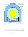
THE BOREXINO DETECTOR ................................................................................... 31
BOREXINO DESIGN ..................................................................................................................... 31
External backgrounds........................................................................................................... 32
Internal backgrounds............................................................................................................ 34
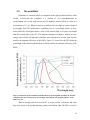
THE SCINTILLATOR..................................................................................................................... 36
BACKGROUND SUBTRACTION ..................................................................................................... 39
Pulse Shape Discrimination ................................................................................................. 39
Delayed coincidence and Statistical subtraction .................................................................. 41
THE COUNTING TEST FACILITY (CTF) ....................................................................................... 42
BOREXINO EXPECTED PERFORMANCE......................................................................................... 44
CHAPTER 4:
INTERNAL SOURCE CALIBRATION ..................................................................... 48
4.1
PSD SPATIAL DEPENDENCE ........................................................................................................ 49
4.1.1
The Monte Carlo................................................................................................................... 50
4.1.2
Alpha/beta separation spatial dependence ........................................................................... 53
4.1.3
Conclusion............................................................................................................................ 58
4.2
METHOD .................................................................................................................................... 58
4.2.1
Design................................................................................................................................... 59
4.2.2
Alpha source ......................................................................................................................... 62
4.2.3
Beta source ........................................................................................................................... 63
CHAPTER 5:
5.1
5.2
5.3
5.4
5.5
SOURCE INSERTION SYSTEM (SIS)....................................................................... 65
INSERTION RODS ........................................................................................................................ 67
THE UMBILICAL CORD ................................................................................................................ 69
THE GLOVE-BOX AND THE SOURCE CHANGING BOX ................................................................... 70
COUPLING TO THE FILLING STATIONS AND OPERATION .............................................................. 73
CONTAMINATION CONCERNS...................................................................................................... 76
CHAPTER 6:
SOURCE LOCATION SYSTEM................................................................................. 78
6.1
MOTIVATION (BOREXINO’S SOLAR NEUTRINO SIGNATURE) ....................................................... 79
6.2
CONCEPTUAL DESIGN ................................................................................................................. 79
6.2.1
Ray tracing ........................................................................................................................... 80
6.2.2
Triangulation ........................................................................................................................ 83
v
6.3
6.3.1
6.3.2
6.3.3
6.4
6.4.1
6.4.2
6.5
6.5.1
6.5.2
6.6
6.7
6.8
6.9
ACTUAL DESIGN ......................................................................................................................... 83
The camera housing.............................................................................................................. 84
The camera assembly............................................................................................................ 86
Radioactivity of materials..................................................................................................... 92
CONTROL SYSTEM AND SOFTWARE ............................................................................................ 93
Control box........................................................................................................................... 94
Control software ................................................................................................................... 96
CALIBRATION, IMAGE ANALYSIS, AND SOURCE LOCATING ....................................................... 103
Calibration ......................................................................................................................... 104
Source locating software .................................................................................................... 107
MAY 2002 TEST........................................................................................................................ 113
ADDITIONAL USES .................................................................................................................... 115
CTF CAMERAS ......................................................................................................................... 119
CONCLUSIONS .......................................................................................................................... 122
CHAPTER 7:
OTHER CALIBRATION SYSTEMS ........................................................................ 125
7.1
PMT CALIBRATION .................................................................................................................. 125
7.2
BUFFER AND SCINTILLATOR CALIBRATION ............................................................................... 128
7.2.1
Internal optical source........................................................................................................ 128
7.2.2
External optical sources ..................................................................................................... 130
7.3
EXTERNAL GAMMA SOURCE CALIBRATION SYSTEM ................................................................. 132
CHAPTER 8:
CONCLUSION ............................................................................................................ 137
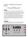
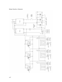
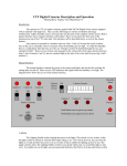
APPENDIX A – CTF DIGITAL CAMERAS DESCRIPTION AND OPERATION ......................... 140
REFERENCES ......................................................................................................................................... 150
vi
List of figures:
Figure 2.1: Two-body decay.
5
Figure 2.2: Three-body decay.
7
Figure 2.3: Electroweak interactions.
12
Figure 2.4: The Higgs mechanism.
13
Figure 2.5: Neutrino Dirac mass.
14
Figure 2.6: Neutrino Majorana mass.
14
Figure 2.7: Electron energy spectrum in beta decay.
16
Figure 2.8: The neutrino is its own anti-particle.
17
Figure 2.9: Diagram for neutrinoless double beta decay.
17
Figure 2.10: MNSP mixing matrix.
19
Figure 2.11: MSW effect in the Sun.
21
Figure 2.12: The pp-chains in the Sun.
23
Figure 2.13: Spectrum of neutrinos expected from the SSM and the respective reactions they are
from [45].
23
Figure 2.14: The expected fluxes for each solar neutrino experiment, and the total measured flux
25
[45].
Figure 2.15: Neutrino mixing parameter space.
26
Figure 2.16: LMA solution.
27
Figure 2.17: Transition from Vacuum to Matter dominated oscillations.
28
Figure 3.1: BOREXINO design.
33
Figure 3.2: Emission spectra and PMT quantum efficiency.
36
Figure 3.3: Energy levels for π-electrons in the scintillator [52].
37
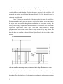
Figure 3.4: Gamma quenching.
38
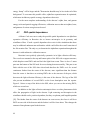
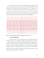
Figure 3.5: Photon time distribution.
39
Figure 3.6: Sample Tail/Total ratio histogram.
40
Figure 3.7: Tail to Total ratio from the CTF [54].
40
Figure 3.8: The
238
U and
232
Th chains.
41
Figure 3.9: Original CTF.
43
Figure 3.10: Borexino Monte Carlo fitted spectrum before cuts.
45
Figure 3.11: Borexino Monte Carlo fitted spectrum after cuts.
45
Figure 3.12: Hypothetical spectrum with poor alpha/beta separation.
47
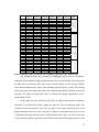
Figure 4.1: Layout of holes on Borexino SSS.
50
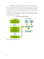
Figure 4.2: Borexino global code structure.
51
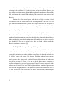
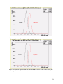
Figure 4.3: Alpha/beta separation with 25ns time threshold for tail for 450 keV events.
54
Figure 4.4: Alpha/beta separation with 25ns time threshold for tail for 750 keV events.
54
vii
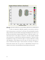
Figure 4.5: Contour plot of tail/total ratio versus total number of photoelectrons for both 450 and 750
55
keV events.
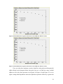
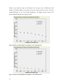
Figure 4.6: Threshold ratio to tag 95% of the betas versus radius (for 450 keV events).
56
Figure 4.7: Threshold ratio to tag 95% of the betas versus radius (for 750 keV events).
56
Figure 4.8: Ratio of residual alphas to total alphas versus radius (450 keV).
57
Figure 4.9: Ratio of residual alphas to total alphas versus radius (750 keV).
57
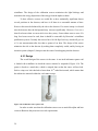
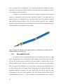
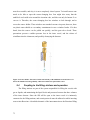
Figure 4.10: Calibration source quartz vial.
59
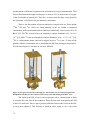
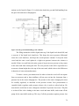
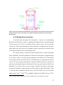
Figure 4.11: Source loading station schematic.
60
Figure 4.12: Prototype source loading station to create 222Rn sources.
61
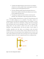
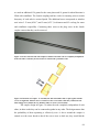
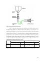
Figure 4.13: Beta calibration source micro-capillary tube.
63
Figure 5.1: Cleanroom 4 (CR4).
66
Figure 5.2: Cylinder mapping in IV.
67
Figure 5.3: Source insertion rod with couplers welded on.
68
Figure 5.4: Insertion rod coupler.
68
Figure 5.5: Hinge rod.
69
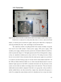
Figure 5.6: SIS glove-box and source-changing box.
71
Figure 5.7: Source-changing box.
72
Figure 5.8: The sliding seals.
72
Figure 5.9: Source holder.
73
Figure 5.10: SIS gas and fluid handling system schematic.
74
Figure 6.1: Image distortions due to lens geometry.
80
Figure 6.2: Illustration of simulated camera.
82
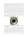
Figure 6.3: Drawing of camera housing, which is mounted on the SSS.
84
Figure 6.4: Effective pinhole determination.
85
Figure 6.5: Camera assembly.
86
Figure 6.6: Lens/camera mount.
88
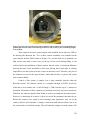
Figure 6.7: Borexino picture with vessels.
90
Figure 6.8: Camera assembly mounted inside the camera housing.
92
Figure 6.9: The camera control box.
94
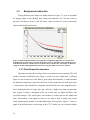
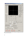
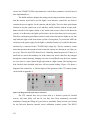
Figure 6.10: Main window for the software.
96
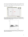
Figure 6.11: Camera Control window for general pictures.
98
Figure 6.12: Camera Control window for taking calibration source photos.
98
Figure 6.13: Associate Cameras window.
100
Figure 6.14: Camera parameter menu.
102
Figure 6.15: Load camera parameters.
103
Figure 6.16: Fit menu.
105
Figure 6.17: Simulated camera photo fitted to actual photo.
106
viii
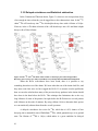
Figure 6.18: Vector representation of the fit residuals.
107
Figure 6.19: Image analysis interface.
109
Figure 6.20: Image noise reduction.
110
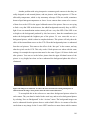
Figure 6.21: LED test string in Borexino.
113
Figure 6.22: Histogram of the radial errors for the LED positions and the fitted probability density
function.
115
Figure 6.23: Calculated error in water level.
117
Figure 6.24: Movie of water filling.
118
Figure 6.25: CTF Camera housing with camera installed.
120
Figure 6.26: Diagram of the CTF camera control box.
121
Figure 6.27: Pictures from the CTF cameras.
122
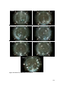
Figure 6.28: Pictures from Borexino's seven cameras.
124
Figure 7.1: The PMT quantum efficiency with the emission spectra of pseudocumene and scintillator
[52].
126
Figure 7.2: The Two Liquid Test Tank (TLTT).
128
Figure 7.3: The internal optical source.
130
Figure 7.4: Radial beams feed-through including the lens mount and pinhole collimator [52].
131
Figure 7.5: Aiming system for the oblique beams system.
132
Figure 7.6: Radial distribution of simulated events from a
228
Th source 635 cm from center of
detector [52].
Figure 7.7: Energy distribution of simulated events from a
133
228
Th source located 635 cm from center
of detector.
134
Figure 7.8: External source reentrant tube.
135
Figure 7.9: External source insertion system.
136
ix
List of tables:
Table 2.1: Table of the elementary particles and some of there properties.
11
Table 2.2: The electroweak charges of the known leptons.
12
Table 2.3: The electroweak charges including right-handed neutrinos.
14
Table 2.4: Proposed future neutrino-less double beta decay experiments.
18
Table 4.1: Simulation source coordinates.
52
Table 4.2: Possible alpha sources for calibration [60].
62
Table 4.3: Beta isotopes for calibration source.
64
Table 6.1: Camera specification for the Kodak DC290 Digital Zoom Camera.
87
Table 6.2: Camera cabling.
91
Table 6.3: Radioactive impurities in camera housing and camera assembly.
93
Table 6.4: Publication featuring CTF and Borexino pictures using Virginia Tech cameras.
Table 7.1: Rates predicted for a
x
228
Th source located 635 cm from the center of the detector.
119
136
List of equations:
Equation 2.1: Number of active light neutrinos [14].
10
Equation 6.1: Polynomial to correct the distortions in the images due to the lenses.
81
Equation 6.2: Sum of squares of distances from the presumed LED position and the point on the ray
which is closest to the LED position.
83
xi
Chapter 1:
Introduction
The neutrino (ν) was introduced nearly three quarters of a century ago [1], and has
remained quite elusive. It took a quarter of a century between prediction and discovery
[2], and we are still probing its basic properties today. The Sun, as a nuclear furnace,
provides a very strong source for electron-type neutrinos (νe). The neutrino has a very
small interaction probability and therefore the ones emitted by the Sun’s core travel
through the Sun and arrive at the Earth uninhibited. This makes the solar neutrino a
perfect probe of the Sun’s core, and has been studied for many decades.
In 1968 Raymond Davis built the first solar neutrino detector to study the Sun’s
core [3], but he measured less than 30% of the expected flux predicted by the solar model
[4,5]. This became known as ‘the solar neutrino problem’, and prompted more
experiments [6,7,8,9,10], which all measured a deficit in the solar neutrino flux.
However, this can be explained if the neutrino is not in a mass eigenstate, but is instead a
superposition of mass eigenstates. This property can lead to neutrino oscillations, which,
if true, would allow the νe born in the Sun’s core to morph into another flavor neutrino
(νµ, ντ) before they reach the Earth. The solar neutrino detectors up to this point were
primarily sensitive to the νe, which would explain why they have been measuring a solar
neutrino flux lower than expected if the neutrinos are oscillating.
The Sudbury Neutrino Observatory (SNO) [11] became the first detector to be
able to measure all flavors of neutrinos and differentiate the νe from the other flavors.
Therefore, giving it the possibility to measure the total neutrino flux, compared to only
the νe flux. In 2002 SNO showed that the total number of neutrinos reaching the Earth
match what the Standard Solar Model predicts [12], and that the neutrinos are changing
flavor before reaching the Earth.
Neutrino oscillations require not only a non-zero neutrino mass, but a non-zero
mixing angle. Currently a global fit to all the existing solar neutrino data, including SNO
and KAMLand [13] (a reactor-neutrino experiment), shows very strong evidence for a
solution in the mass-mixing angle phase space called the Large Mixing Angle (LMA)
1
solution [14]. This solution requires a matter enhanced oscillation mechanism called the
MSW effect [15,16], which comes about because solar νe interact differently than νµ and
ντ in an electron dense material.
Borexino is a liquid scintillator detector designed specifically to measure the
neutrinos produced in electron capture of 7Be in the core of the Sun, the so-called 7Be
neutrino [17]. This neutrino can be measured in real-time and has an energy of 863 keV,
which is far below the lower threshold of SNO and Super-Kamiokande [10] (another
solar neutrino detector), which are the only detectors with information about the solar
neutrino energy spectrum. When Borexino was first developed, its primary charge was to
measure the oscillation parameters θ12 (mixing angle) and ∆m122 ≡ m12 − m22 (mass
differences between the mass eigenstates), and to find which of the several possible
solutions to the solar neutrino deficit was correct. Borexino will be able to confirm the
LMA solution result independently of other experiments and put better limits on the
mixing angle. However, Borexino’s charge has changed somewhat over the years and
other possible caveats in solar neutrino physics have come to light, which Borexino will
be able to explore.
If the LMA solution is correct, then neutrinos at lower energy will be dominated
by vacuum oscillations and not matter enhanced oscillations (MSW effect), which is the
main mechanism at the higher energies. Existing higher energy spectral data cannot probe
this transition, but the neutrino energy that Borexino will study is vacuum oscillation
dominated, if this effect is true. Borexino will also be able to provide some insight to the
luminosity constraint, which is the direct correlation between the radiative energy and the
neutrino energy emitted from the Sun.
The Borexino experiment measures the neutrinos through neutrino-electron
scattering in liquid scintillator [17]. This reaction does not have a very unique signature
and can be mimicked by alpha, beta, and gamma radiations. The energy of the 7Beneutrino falls in an energy range where natural radioactivity becomes the limiting
background. Uranium and Thorium are the major culprits, along with their many alpha
and beta emitting daughters. The background must be as low as possible to extract the
7
Be-neutrino flux, so event tagging of the background is necessary. Pulse shape
discrimination is required to identify alphas in the detector, and it is possible to tag
2
daughters of the Uranium-238 and Thorium-232 chains with a time delayed coincidence.
A statistical subtraction can then be used to further lower the background. However, the
pulse shape discrimination’s efficiency is position dependent due to known and unknown
anisotropies in the detector. To remove the background events properly, the position
dependencies must be understood precisely.
To find the efficiency of the alpha/beta separation as a function of position and
energy we use alpha and beta calibration sources of various energies. These sources can
be placed throughout the detector with an insertion system developed at Virginia Tech,
and their positions can be found independently of the photomultiplier tubes to a high
accuracy with an independent location system. We have also made significant strides
towards the development of these sources. This dissertation provides motivation for the
use of radioactive sources, and reports on the development of the insertion and location
systems.
The dissertation is organized as follows:
Chapter 2 will begin by describing why the neutrino was introduced and how it
was found. Then we will briefly introduce neutrino properties and how mass enters into
the elementary particles and what consequence a massive neutrino has on particle
physics. The influence solar neutrinos have had on the search for the neutrino properties
will then be described, and finally we will give motivation for what a 7Be-neutrino can
teach us about neutrino mass and solar physics.
Chapter 3 will give us a description of the Borexino detector. This will include
both the detector geometry and how it will measure the flux of 7Be-neutrinos. The
backgrounds and their reduction techniques will be detailed and finally the expected
performance of Borexino will be presented. This will give the basic motivation for
radioactive source calibration.
Alpha/beta separation based on pulse shape discrimination is one of the major
background reduction techniques. Chapter 4 presents a study performed on the spatial
dependence of alpha/beta separation, which gives further in-depth motivation for
radioactive calibration sources. We will also describe the design for the sources and list
possible sources and what can be learned from them.
3
Chapter 5 details the Source Insertion System, which is used to introduce and
manipulate the calibration sources in the detector. All the designs and concerns for every
component in the system are described, and the procedure for inserting sources will also
be described.
Chapter 6 contains everything about the source location system, which is needed
because the insertion system cannot provide the source location accurately enough. In
order to find the source position independently of the photomultiplier tubes, digital
cameras are used to find the source position to better than 2 cm anywhere in the detector.
These cameras can also be used for several other purposes, which will also be described
Chapter 7 will give a brief overview of the other calibration systems in place.
Because of the invasive nature of the radioactive sources, other calibration systems exist
to measure properties of the detector that the radioactive sources are not required for.
Chapter 8 will provide conclusions and outlook, with a brief explanation of the
August 2002 Borexino accident.
4
Chapter 2:
Neutrino Physics
Our understanding of nuclear and particle physics changed drastically when the
neutrino was introduced over 70 years ago. Since then we have learned many things
about the neutrino and how the other elementary particles interact, culminating in the
construction of the Standard Model. However, it is only within the past decade that
experiments have started to yield answers to such basic questions as “do neutrinos have
mass?”, and now it looks like the neutrino is on the verge of changing particle physics
again.
Solar neutrinos have played an important role in this development. Over 35 years
ago a deficit in the solar neutrino flux was found, and in 2001 SNO [11,18] finally found
direct evidence that these neutrinos were changing flavor. SNO put very stringent limits
to the neutrino mass parameters, but further studies of the solar neutrinos at much lower
energies will be able to further expand our knowledge of the neutrino, and finally answer
the question Ray Davis asked in 1968 with the first solar neutrino experiment, how does
the Sun work?
2.1
Neutrino hypothesis and discovery
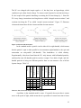
2.1.1 Beta decay problem
At the beginning of the twentieth century, a problem arose with the electron
energy spectrum in Beta decay. Beta decay, at the time, was understood as an atom
changing into another atom by releasing an electron, which is a two-body decay (Figure
2.1).
Figure 2.1: Two-body decay.
Energy and momentum conservation require the electron in this beta decay to be monoenergetic. However, in 1913 James Chadwick, while at the University of Berlin, studied
5
the beta ray spectrum of Radium B+C and found a continuous spectrum for the emitted
electron, without the peaks that other measurements had seen [19]. To explain this Niels
Bohr had gone so far as to suggest that energy might not be conserved [20].
After Rutherford discovered the atomic nucleus [21] it was believed that the
nucleus of an atom consisted of electrons and protons. The neutron had not been
discovered at this point. Rather than using neutrons and protons to obtain the correct
mass and charge, only protons were added together to obtain the correct mass, and then
electrons were used to cancel the proton’s charge to match the charge of the nucleus. For
example, the nitrogen-14 nucleus has a mass of 14 atomic mass units (amu) and a charge
of +7e, where e is the elementary charge (1.6022 x 10-19 Coulomb); according to the
above theory, the
14
N nucleus consists of 14 protons and 7 electrons. This theory also
described beta decay simply as the release of an electron from the nucleus.
Another problem that was coming into light at the time was the problem of spin.
If the proton-electron model of the nucleus were true then a nucleus needed to have
enough protons to give the right charge, and enough proton-electron pairs to give the
right mass. The spin of the resultant nucleus would have either whole or half-integer spin,
because the electron and the proton both have spin-½. The problem was found with the
Nitrogen-14 nucleus. The proton-electron model says that this nucleus consists of 14
protons and 7 electrons, for a total of 21 spin-½ particles together equaling a half-integer
spin nucleus. In 1929, Franco Rasetti, at the California Institute of Technology, found
that the 14N nucleus has a spin equal to one [22], but this is not possible if the nucleus has
21 spin-½ constituents.
2.1.2 Pauli’s Neutronen
Enter Wolfgang Pauli. To solve the problems of electron energy in beta decay,
and the nuclear spin, Pauli suggested a new particle he named a “neutronen”, or neutron*
in German. The neutronen was first proposed in a letter Pauli wrote to his colleagues at a
workshop in Tübingen on December 4, 1930. A translation of the letter Pauli wrote to
these members is shown here as translated in reference [23], (Reprinted with permission
from L. M. Brown, “The idea of the neutrino”, Physics Today, September 1978, p23,
*
The Neutron was not discovered until 1932 by James Chadwick [24]
6
Copyright 1978, American Institute of Physics). The neutron mentioned in this letter does
not refer to James Chadwick’s neutron, but to Pauli’s neutronen.
Dear radioactive ladies and gentlemen,
As the bearer of these lines, to whom I ask you to listen graciously, will explain
more exactly, considering the “false” statistics of N-14 and Li-6 nuclei, as well as the
continuous β-spectrum, I have hit upon a desperate remedy to save the “exchange
theorem” of statistics and the energy theorem. Namely [there is] the possibility that there
could exist in the nuclei electrically neutral particles that I wish to call neutrons, which
have spin ½ and obey the exclusion principle, and additionally differ from light quanta in
that they do not travel at the velocity of light: The mass of the neutron must be of the
same order of magnitude as the electron mass and, in any case, not larger than 0.01
proton mass. – The continuous β-spectrum would become understandable by the
assumption that the sum of energies of the neutron and the electron is constant.
Now the next question is what forces act upon the neutrons. The most likely
model for the neutron seems to me to be, on wave mechanical grounds (more details are
known by the bearer of these lines), that the neutron at rest is a magnetic dipole of a
certain moment µ. Experiment probably requires that the ionizing effect of such a neutron
should not be larger than that of a γ ray, and thus µ should probably not be larger than
e.10-13 cm.
But I don’t feel secure enough to publish anything about this idea, so I first turn
confidently to you, dear radioactives, with the question as to the situation concerning
experimental proof of such a neutron, if it has something like about 10 times the
penetrating capacity of a γ ray.
I admit that my remedy may appear to have a small a priori probability because
neutrons, if they exist, would probably have long ago been seen. However, only those
who wager can win, and the seriousness of the situation of the continuous β-spectrum can
be made clear by saying of my honored predecessor in office, Mr. Debye, who told me a
short while ago in Brussels, “One does best not to think about that at all, like the new
taxes.” Thus one should earnestly discuss every way of salvation. –So, dear radioactives,
put it to the test and set it right. –Unfortunately I cannot personally appear in Tübingen,
since I am indispensable here on account of a ball taking place in Zürich in the night
from 6 to 7 December. –With many greetings to you, also to Mr. Back, your devote
servant,
W. Pauli
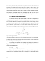
With Pauli’s neutronen as a constituent of the nucleus beta decay is understood to
be a three-body decay (Figure 2.2). Now it is possible to have a continuous electron
energy spectrum in beta decay, with the neutronen carrying away part of the energy
undetected. The
14
N spin problem was also solved by having 7 protons, 14
proton/electron pairs and an odd number of neutronens. Now, there were an even number
of spin-½ particles that could add up to a spin one nucleus.
Figure 2.2: Three-body decay.
7
In 1932 James Chadwick discovered the neutron, and the picture we had of the
nucleus changed forever [24]. As mentioned earlier, up until two years prior, it was
believed that the nucleus of the atom was made up of electrons and protons, and Pauli’s
neutronen was just a hypothetical particle. Nature was believed to be simple, and
suggesting that there were more than just three elementary particles as the building
blocks of matter was not heading in the right direction. Pauli had been afraid to publish
his idea of the neutronen, and Chadwick also resisted suggesting that the neutron was an
elementary particle. Dmitri Iwanenko and Werner Heisenberg changed all this. Iwanenko
in a paper took the leap to say that the neutron was an elementary particle [25].
Heisenberg’s proton-neutron model changed the way we thought of the atomic nucleus
[26]. Heisenberg completely removed the electrons from the nucleus, thereby proposing
that the electron, in beta decay, was created during the decay, and not simply released
from the nucleus. This was not so crazy, for another elementary particle was known to be
created, namely the photon, and Dirac had worked extensively on the quantum mechanics
of its creation in the 1920s. While at the Niels Bohr Institute in 1926, Dirac wrote the
first paper on quantum electrodynamics that describes the creation and annihilation of
photons [27].
In 1933, Fermi combined Heisenberg’s neutron-proton model of the nucleus,
Pauli’s neutronen, and Dirac’s idea of creation and annihilation to form the now famous
Fermi’s theory of beta decay. This theorized that the neutron converted into a proton by
emitting an electron and a neutrino [28]. Fermi was the first to coin the term neutrino,
meaning “little neutral one”, since Chadwick had used neutron to describe his heavy
neutral particle.
Although Bethe and Peierls had calculated the neutrino cross-section to be less
than 10-44 cm2 [29], it was now time to find the neutrino experimentally. This would not
happen until two decades latter.
2.1.3 Hanford and Savannah River experiments
In 1953 Fred Reines and Clyde Cowan set up a detector near the nuclear reactor
in Hanford Washington to measure the neutrinos emitted from the reactor’s core. At the
time the anti-neutrino was not known, which is actually what is created in a reactor.
8
Antineutrinos inverse beta decay with protons in the detector to create a positron and a
neutron.
ν e + p → e+ + n
The positron annihilates with an electron producing two gamma rays in the detector’s
liquid scintillator and the neutron later captures on the Cadmium (Cd) dissolved in the
scintillator, which produces gammas.
e + + e − → γ + γ and n+ ACd → ( A + 1) Cd + γ ' s
This gave the experimenters a delayed coincidence to tag neutrino events. The problem
was the background from cosmic rays, which produced false coincidences, and in the end
a definitive identification of neutrino detection could not be made [30].
To confirm the results of the experiment at the Hanford reactor, a second larger
experiment was built near the newly constructed Savannah River nuclear reactor in South
Carolina. The Hanford experiment had relied on the inverse beta decay reaction taking
place inside a single volume where accidental coincidences could take place. To
overcome this in the Savannah River experiment, Reines and Cowan used a sandwich
detector configuration. Two tanks containing cadmium chloride in a water solution acted
as the target for the neutrino. Here, the neutrino would convert a proton to a neutron and
emit a positron. The positron would quickly annihilate with an electron and produce two
gamma rays. The neutron would then capture on the cadmium with a characteristic time,
and would produce gamma rays. These cadmium loaded water tanks sat between three
liquid scintillator layers where the gammas would be detected. This experiment was able
to efficiently tag the neutrino events in the water/cadmium target by looking for
coincidences between the two scintillation counters on either side of the target. The
Savannah experiment confirmed the Hanford reactor experiment, proving for the first
time that neutrinos exist [31]. In 1995, Fred Reines was awarded the Noble Prize in
physics for the detection of neutrinos at Hanford.
2.1.4 More than one neutrino
In 1937 a new particle was found which showed the same properties of the
electron but with a far greater mass, the muon (µ) [32], and in 1962 a neutrino associated
with the muon was found [33], which earned Leon Lederman the Nobel prize in physics
9
in 1988. The neutrino that Reines found was associated with the electron and is now
called the electron neutrino (νe); in other words, it carried an electron flavor whereas
Lederman’s neutrino carried muon flavor and is called the muon neutrino (νµ). The muon,
electron, and their associated neutrinos are part of a family of particles called leptons. In
1975, a third charged lepton was found with a very heavy mass (~1.8 GeV), which was
named the Tau lepton (τ). Since the other leptons have neutrinos associated with them, it
was assumed that there also existed a tau neutrino (ντ), and it was detected by the
DONUT collaboration in 2001 [34]. But how do we know that there aren’t more flavors
of neutrinos?
By studying the width and the total mass of the Z boson produced in e+ecollisions, it is possible to discern how many flavors of active light neutrinos there are
(“light neutrinos” are defined as having a mass less than half the Z mass). First we need
to measure the partial width of decays which are not seen in the detector, but are known
to exist. This invisible partial width Γinv is found by subtracting all the measured partial
widths from the total width of the Z, and is assumed to be due to neutrino events. So, if
one takes the ratio of Γinv to the charge lepton partial width Γl, we can compare that to the
calculated ratio of the neutrino partial width Γν and charged lepton partial width. From
this, one obtains the number of neutrino flavors Nν to be:
Nν =
Γinv
Γl
 Γl

 Γν

 = 2.994 ± 0.012
 SM
Equation 2.1: Number of active light neutrinos [14].
2.2
Neutrinos in the Standard Model and Beyond
Fermi’s theory of beta decay was very successful, but it is not complete. At higher
energies it is not able to predict the outcome of reactions accurately enough. To explain
the interaction between the elementary particles at higher energies, the Standard Model of
Fundamental Particles and Interactions (the standard model) was developed. The standard
model reduces to Fermi’s theory in the low energy limit. It contains all the fundamental
particles, which form the universe we live in, and describes all the interactions among
them. Table 2.1 shows a list of all the particles in the standard model, and some of their
properties.
10
Flavor
νe
e
νµ
µ
ντ
τ
Fermions matter constituents
Spin 1/2, 3/2, 5/2, …
Leptons spin = ½
Quarks spin = ½
Mass
Electric
Flavor
Aprox. Mass
(GeV/c2)
Charge
(GeV/c2)
< 3×10-9
0
0.0015 to 0.0045
u
0.000511
-1
0.004 to 0.008
d
<0.00019
0
1.15 to 1.35
c
0.1056
-1
0.080 to 0.130
s
174.3 direct observation of t
t
<0.0182
0
1.777
b
-1
Electric
Charge
178.1 Standard model EW fit
4.1 to 4.4 ( MS mass)
4.6 to 4.9 (1S mass)
Bosons force carriers
Spin 1, 2, 3, …
Unified Electroweak spin = 1
Strong (color) spin = 1
< 6×10-17 ≈ 0
< 5×10-30 ≈ 0
0
γ
g
80.4
-1
W
80.4
+1
All values taken from [14]
W+
0
91.18
0
Z
2/3
-1/3
2/3
-1/3
2/3
-1/3
0
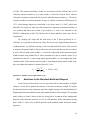
Table 2.1: Table of the elementary particles and some of their properties.
There are three fundamental forces in the standard model. The strong force holds
quarks together to form Baryons (protons, neutrons, etc.) and Mesons (pions, Kaons,
etc.). The weak force and the electromagnetic force are just manifestations of a combined
electroweak force, which drives such things as beta decay. The neutrino only interacts
through the weak force.
2.2.1 Interactions of the Standard Model
The standard model describes interactions as the exchange of force carriers, which
couple to “charges” the elementary particles carry. These charges are conserved
quantities, which must remain constant through the reaction. The force carriers in the
standard model are the bosons, which are emitted or absorbed in every interaction.
In the electroweak force, there are two charges and four force carriers. The W+
and W- bosons couple to the isospin (I3) of the particle, while the Z0 couples to both
isospin and hypercharge. The photon (γ) couples to electric charge (Q), which is a
combination of isospin and hypercharge (Y).
Q = e(I3 + Y/2)
11
The W’s are charged with isospin equal to ±1, but they have no hypercharge, which
combines to give them electric charge. To conserve total isospin of a reaction involving a
W, the isospin of the particle absorbing or emitting the W must change by 1. Since the
W’s carry charge, interactions involving them are called “charged current reactions”, and
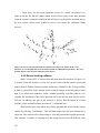
reactions involving the Z0 are called “neutral current reactions”. Figure 2.3 illustrates
electroweak interactions for the electron and the electron neutrino.
Figure 2.3: Electroweak interactions.
In the standard model a particle can be either left or right handed, which means
that the particle’s spin is either parallel to its momentum (right-handed) or the spin and
momentum are anti-parallel (left-handed). This handedness is called chirality.
Experimentally it has been found that the W’s only interact with left-handed particles,
and therefore only left-handed particles can have isospin. If we think of right- and lefthanded particles as being two different particles then we can construct a list of all the
leptons charges, Table 2.2.
-1
-1
-1
-1
-1
-1
Electric charge
(in units of e)
-½
-½
-½
½
½
½
Hypercharge (Y)
eL
µL
τL
νeL
νµL
ντL
Isospin (I3)
Particle
Electric charge
(in units of e)
Hypercharge (Y)
Isospin (I3)
Particle
left-handed
right-handed
-1
-1
-1
0
0
0
eR
µR
τR
0
0
0
-2
-2
-2
-1
-1
-1
Table 2.2: The electroweak charges of the known leptons.
A problem in the standard model is mass. If a particle has mass then it cannot
move at the speed of light, which means that it is possible to Lorentz boost into a frame
12
that is moving faster than the particle. When we perform such a boost the momentum of
that particle will change direction, but the spin will not, which is a flip in chirality. This
indicates that a massive particle cannot have definite chirality. It is a mixture of both leftand right-handed components. Indeed, mass is actually a chirality changing interaction,
which changes a left-handed particle into a right-handed one, and vise versa. Such a
transition demands that the isospin changes by ±½, which violates isospin conservation.
2.2.2 Masses in the Standard Model
To incorporate mass into the standard model we must have a mechanism for
changing the particle isospin by ±½ without violating isospin conservation. We can do
this if we assume that there is an infinite sea of isospin available. A new isospin-½ boson
is introduced which couples the left- and right-handed particles together. When this
boson “condenses” in the vacuum, it acts as the infinite isospin reservoir (Figure 2.4).
This is known as the Higgs mechanism, and the new boson is called the Higgs boson (φ).
Figure 2.4: The Higgs mechanism.
The Higgs mechanism is able to give all the fermions their masses. In this mechanism,
the Higgs boson carries isospin from the isospin sea to the particle, or takes isospin from
the particle and gives it to the isospin sea.
The exception is the neutrino. Since neutrinos were thought to be massless, no
Higgs mechanism for the neutrino was assumed, and the right-handed neutrinos were not
included in the standard model.
2.2.3 Dirac and Majorana masses
Evidence for neutrino mass has grown over the years, which requires the
introduction of the right-handed neutrino and its coupling to the left-handed neutrino
13
through the Higgs. By definition the right-handed neutrino has no isospin, electric charge,
and hypercharge (Table 2.3).
-1
-1
-1
-1
-1
-1
Electric charge
(in units of e)
-½
-½
-½
½
½
½
Hypercharge (Y)
eL
µL
τL
νeL
νµL
ντL
Isospin (I3)
Particle
Electric charge
(in units of e)
Hypercharge (Y)
Isospin (I3)
Particle
left-handed
right-handed
-1
-1
-1
0
0
0
eR
µR
τR
0
0
0
-2
-2
-2
-1
-1
-1
νeR
νµR
ντR
0
0
0
0
0
0
0
0
0
Table 2.3: The electroweak charges including right-handed neutrinos.
The chargeless right-handed neutrinos cannot be observed at all, because all the force
carriers have nothing to couple to, except through the Higgs. These neutrinos will be
completely invisible until it becomes left-handed through the Higgs again. The mass the
neutrino acquires through the Higgs mechanism is called a Dirac mass (Figure 2.5).
Figure 2.5: Neutrino Dirac mass.
An observed conservation in the leptons is a quantity called lepton-number (L).
Each lepton has L = 1 and the anti-leptons have L = -1. There is only experimental
evidence for this conservation, because there is no “flavor” charge on the leptons that a
force couples to. If we allow lepton-number violation then the right-handed neutrino
could change into its own anti-particle, which would be left-handed. This transition is
also a chirality flip, i.e. a mass called a Majorana mass.
Figure 2.6: Neutrino Majorana mass.
14
A Majorana mass is unique to the right-handed neutrino, and its anti-particle. For all the
other particles of the standard model a Majorana mass would violate charge conservation.
We can now write done the complete mass term for the neutrino.
[ν L
mD  ν L 
+ h.c.
M R  ν R 
 0
mD
ν R ]
where mD are the Dirac masses and MR is the Majorana mass term. A non-zero ML
requires isospin to change by one unit, but the Higgs can only change isospin by ½.
By diagonalizing the mass matrix, we can describe the neutrino masses as pure
Majorana masses, even if MR = zero. The mass eigenvalues corresponding to the
eigenstates of the diagonalized mass matrix are:
m1, 2 =
1
2
[(M ) ±
R
M R2 + 4mD2
]
If we also assume that MR >> mD, as suggested by Grand Unified Theories, then
we find that the lighter mass eigenvalue is mν ≈ − mD mR−1m D . This tells us that if the
Majorana mass is very large, then the measurable neutrino mass will be very small even
if the Dirac mass were comparable to the charged leptons. This is the so-called See-saw
mechanism, which explains why the neutrinos have such small masses compared to the
other leptons.
2.2.4 Neutrino mass measurements
A method to measure the absolute mass of the νe is to look at the end-point of the
beta decay spectrum. This will actually give us the mass of the ν e , but we have no reason
to believe that their masses are different. As we described earlier, beta decay is a threebody decay where all three particles share the energy and momentum of the parent. Since
the parent and daughter nuclei are much more massive than the electron and neutrino, we
can assume that all the kinetic energy goes into the electron and neutrino. If the neutrino
does not have a mass, then it is possible for the electron to receive all the kinetic energy.
However, if the neutrino has a mass then some of the total energy must go into the
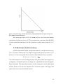
neutrino mass. Figure 2.7, illustrates how the electron energy spectrum will change if the
ν e had a mass, compared to the massless case.
15
Figure 2.7: Electron energy spectrum in beta decay. The maximum kinetic energy the electron can
have depends on the neutrino mass.
The current upper limit of 3eV for the ν e mass has come from such endpoint
experiments of tritium beta decay [14]. The next generation experiment called KATRIN
is under construction and hopes to be able to measure a neutrino mass of only 0.2 eV/c2
[35].
2.2.5 Neutrinoless double beta decay
A nucleus with atomic number A and proton number Z is not able to beta decay to
a (Z+1,A) nucleus if that nucleus is at a higher energy than the parent, but if the (Z+2,A)
nucleus is at a lower energy than the (Z,A) nucleus, then double beta decay is possible,
(Z , A) → (Z
+ 2, A) + 2e − + 2ν e
Now if the neutrino has a non-zero Majorana mass term (MR), then an interesting process
can happen. A left-handed neutrino can change into a right-handed neutrino through the
Higgs mechanism. This right-handed neutrino can then change into an anti-right-handed
neutrino, because of its non-zero Majorana mass. It can then couple to the Higgs field
again, and become an anti-left-handed neutrino.
16
Figure 2.8: The neutrino is its own anti particle. If the lepton number conservation is violated and the
neutrino has a non-zero Majorana mass then such a transition can occur.
If this process is allowed in double beta decay, the neutrinos can annihilate each
other and give all the kinetic energy to the electrons. This process is known as
neutrinoless double beta decay.
Figure 2.9: Diagram for neutrinoless double beta decay. The neutrinos are only virtual particles and
are not seen in the final state, thereby violating lepton number due to the Majorana mass term.
The only ‘positive’ result for neutrinoless double beta decay comes from the
Heidelberg-Moscow experiment, which used enriched
76
Ge. They claim to have found
28.75 ± 6.86 counts for neutrinoless double beta decay and an effective mass of <mββ> =
440 meV. These results are very controversial so I will refer readers to the original papers
listed in references [36,37,38].
Several experiments are underway, and more are proposed to continue to search
for neutrinoless double beta decay in detectors using greater masses and various isotopes.
Table 2.4 lists the experiments and the proposed isotope.
17
Neutrinoless Double Beta Decay Experiments [39]
Experiment
Isotope
CAMEO
116
CANDLE
48
Experiment
Isotope
GSO
160
Majorana
76
MOON
100
CUORE
130
Te
MPI bare Ge
76
DCBA
82
Se
Nano-crystals
EXO
136
Cd
Ca
COBRA
Gd
Ge
Mo
Ge
various
Super-NEMO
82
GEM
76
Xe
136
GENIUS
76
XMASS
136
Xe
Ge
Ge
Se
Xe
Xe
Table 2.4: Proposed future neutrino-less double beta decay experiments.
2.2.6 Neutrino mixing and the MNSP matrix
If neutrinos have mass then the flavor eigenstates νe, νµ, and ντ need not be mass
eigenstates. In general, a neutrino flavor eigenstate is a superposition of mass eigenstates
νl =
3
∑U
m =1
lm
νm
where Ulm is a unitary mixing matrix. If the Ulm is not the identity matrix and if the mass
eigenvalues are non-degenerate, then a neutrino born with momentum pν at time t=0 will
evolve in time as:
ν l ( x, t )
=
3
∑U
m =1
lm
e i ( pν x − Emt ) ν m
for pν >> mi and Em ≈ pν
≈e
ipν ( x − t )
3
∑U
m =1
lm
e
−i
mi2
t
2 pν
νm
This leads to a phenomenon known as flavor oscillation. If we restrict ourselves to two
neutrinos then our mixing matrix only involves one angle:
ν e 
 ν   cos θ
  = U lm  1  = 
ν 
ν 2   − sin θ
 µ
sin θ  ν 1 
 
cos θ ν 2 
To find the probability that a neutrino born as νe oscillates into a νµ after a distance L,
assuming that the neutrino is traveling at c we get:
18
P (ν e → ν µ ) = ν e ν µ (L )
2
 ∆m 2 L 
= sin 2 θ × sin 2 
× 
E
 4
It implies that after the neutrino has traveled a distance away from its creation point, it is
possible to measure it as a different flavor. In other words, the νe has changed into a νµ,
but this can only happen if there is a nonzero mixing angle θ and squared mass difference
∆m2. In the three neutrino case, a similar mixing matrix occurs but needs three mixing
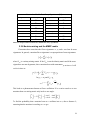
angles and produces two ∆m2ij’s (∆m212 + ∆m223 = ∆m213) in the probabilities.
U lm

c12 c13

=  − s12 c23 − c12 s 23 s13 e iδ
 s c − c s s e iδ
12 23 13
 12 23
c12 c23
s12 c13
− s12 s 23 s13 e iδ
− c12 s 23 − s12 c23 s13 e iδ
s13 e −iδ 

s 23 c13 
c23 c13 
Figure 2.10: MNSP mixing matrix.
where cij=cosθij and sij=sinθij. The eiδ is a CP violating phase. If the neutrinos have nonzero Majorana masses then there will also be two Majorana phases.
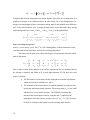
This matrix can be split up to reflect which types of experiments can probe which
parts of the matrix:
U lm
0
1

=  0 c 23
0 − s
23

0  c13

s 23  0
c 23  − s13 e iδ
0 s13 e iδ  c12

1
0  − s12
0 c13  0
s12
c12
0
0

0
1 
This is done because in the analysis of the various experiments the two neutrino limit in
the mixing is assumed, and found to be a good approximation. We list here how each
matrix is studied:
•
The first matrix is associated with the Atmospheric neutrino experiments,
which measure the oscillation of νµ into ντ.
•
The elements of the second matrix are studied primarily by long base-line
accelerator and reactor based neutrinos. The mixing angle θ13 is very small
and therefore is very hard to measure. The CHOOZ experiment has
measured the current upper limit, by using the ∆m132 implied by the
atmospheric and solar neutrino results, to be sin 2 2θ 13 < 0.1 [40]. In order
to find CP violation in the lepton sector this mixing angle must be
19
measurable. When it is found, we can see if CP violation happens in the
lepton sector, or if it is a rarity only seen in the quark sector.
•
The final matrix is represented by the solar neutrino experiments, which
primarily measure the change of νe into νµ.
The types of oscillations discussed so far are called “vacuum oscillations”,
because they occur without the interaction of the neutrino with the surrounding medium.
However when the neutrinos are traveling through electron dense material the νe will gain
an “effective” potential energy which the νµ or ντ will not. This is because the νe can
interact with electrons through the charge current in addition to the neutral current,
whereas the νµ and ντ only interact through the neutral current. The added potential
energy the neutrino in electron density ne sees has the form,
Vν e =
2G f ne
where Gf is the Fermi constant.
If we again only look at the two neutrino case, then we obtain effective masses for
the ν1 and ν2 states in matter.
2
meff
1, 2 =
1
2
(m
2
1
) [(
+ m22 + 2 Eν Vν e ± ∆m 2 cos 2θ − Eν Vν e
)
2
+ ∆m 2 sin 2 2θ
]
1
2
where Eν is the neutrino energy. One still has the same mixing matrix, but this will have
an effect on the survival probability ν e ν e (L ) 2 . We can introduce an effective matter
mixing angle (θm) for the neutrinos in an electron rich atmosphere to see what happens
with different electron densities.
sin 2θ m =
(2
∆m 2 sin 2θ
2G f ne Eν − ∆m 2 cos 2θ
) + (∆m
2
2
sin 2 2θ
)
2
For very low electron densities, the matter mixing angle is nearly equal to the vacuum
mixing angle and the mass eigenvalues are nearly the same. In this case, ν1 is equivalent
to the νe, and ν2 corresponds to νµ. However, when the electron density is very high, then
the matter mixing angle is very large, θm~ π/2, and the correspondence between the mass
and flavor eigenstates is flipped; in other words ν1~ νµ with mass = meff1 and ν2~ νe, with
mass = meff2.
20
A very interesting area is where θm= π/4. At this angle the mixing is maximal.
This resonance will only happen at a specific electron density for a particular neutrino
energy, namely:
∆m 2
cos 2θ
ne (resonant ) =
Eν
2 2G f
1
This is particularly interesting for solar neutrinos. These neutrinos are produced in the
core of the Sun where the electron density is very high. They travel through an ever
decreasing electron density until they reach the surface of the Sun where the electron
density approaches the vacuum. The Sun only produces νe, but at the very high electron
densities this corresponds to ν2 with eigenvalue meff2, which corresponds to νµ at lower
electrons densities. While traveling out from the core, the neutrino will pass through the
resonant density for that energy where the mixing is maximal and if the electron neutrino
stays in the mass eigenstate ν2, it will oscillate into a νµ. Figure 2.11 shows an illustration
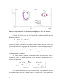
of this effect. This effect is called the Mikheyev-Smirnov-Wolfenstein or MSW effect
[41,42].
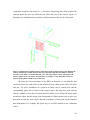
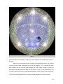
Figure 2.11: MSW effect in the Sun. The resonant electron density allows the electron neutrinos to
oscillate into a muon neutrino with a higher probability than in a vacuum.
21
2.3
Solar neutrinos
Sir Arthur Eddington, in 1926, in an attempt to explain the age of the Sun and the
Solar System, proposed that the Sun does not chemically burn hydrogen, but that there
are other effects that produce energy [43]. Hans Bethe later suggested that this energy
production is nuclear fusion in the Sun’s core and developed the first model to describe
this [44]. The light emitted from the surface of the Sun, which is all we can see, does not
hold the clues to tell us what is happening in its core. Energy produced in the core takes
several tens of thousands of years to reach the surface, which is then sent to the Earth as
light. Helioseismology, which is the measure of sound waves through the Sun, can teach
us many things about the interior of the Sun, but not much about fusion reactions taking
place there. However, if the Sun does have a fusion reactor at its core, then the neutrinos
emitted in those fusion reactions can reveal to us the workings of the Sun’s reactor. The
neutrino’s very small cross-section means that they effectively do not react in the Sun and
can reach the Earth within minutes, since they are nearly massless. Once we understand
the solar interior, we can then use the Sun as a neutrino source to answer some of the
questions about the neutrinos’ mass and mixing, as well as other properties.
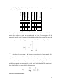
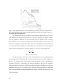
2.3.1 SSM and the solar neutrino problem
The standard solar model (SSM) describes how the Sun works [45]. It models the
delicate balance between gravitational contraction and radiative and particle pressures;
while matching radiative energy output with nuclear fusion energy input. In our case, the
most important part of the SSM is the description of the core of the Sun, and how it burns
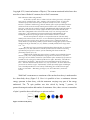
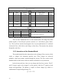
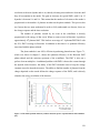
hydrogen into helium through the so called pp-chains. Figure 2.12 shows the pp-chains,
with the reactions marked in red being the ones which produce neutrinos. The predicted
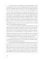
spectrum of the neutrinos from the Sun is shown in Figure 2.13.
22
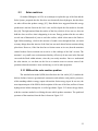
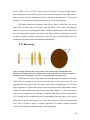
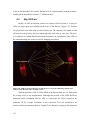
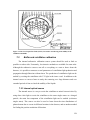
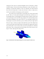
Figure 2.12: The pp-chains in the Sun. This describes energy production in the core.
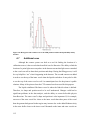
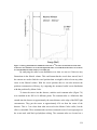
Figure 2.13: Spectrum of neutrinos expected from the SSM and the respective reactions they are
from [45].
23
The Sun is therefore a very good source of neutrinos. In 1968 Ray Davis
measured the flux of neutrinos from the Sun using a radio chemical experiment, and in
2001 was awarded the Nobel Prize in physics for that work. His goal was to probe the
core of the Sun to confirm that it is indeed a nuclear furnace. He made use of the
following reaction to measure the neutrinos:
37
Cl + νe Æ 37Ar + e-
A tank filled with 615 tons of Perchloroethylene was allowed to build up the argon over
several weeks. Then the argon was removed and counted. This resulted in a measurement
of the neutrino flux, which corresponded to about 30% of the SSM prediction [4,5] . This
deficiency in the solar neutrino flux became known as “The Solar Neutrino Problem”.
Several other experiments also measured the flux of neutrinos from the Sun with
similar results. Two more of these experiments used the radio chemical technique;
however this time gallium was used (71Ga + νe Æ 71Ge + e-) in order to lower the energy
threshold. These experiments were the Soviet American Gallium Experiment (SAGE) [6]
and the GALLEX experiment [7], which later became GNO [8]. The radio chemical
experiments have the limitation that they only see an integrated flux above a threshold,
and therefore cannot provide the energy spectrum of the neutrinos they detect. Neither
can they provide any time or directional information.
Initial spectral measurements were made by the Kamiokande [9] and later Super
Kamiokande [10] experiments. They measure the Čerenkov light produced in water by
the recoil of an electron after being hit by a neutrino. However, they can only measure the
flux at energies high enough to produce sufficient Čerenkov radiation in water greater
than background for detection (>5MeV). Up to this point in history, the measured
neutrino flux was still far below the expected value predicted by the SSM. Figure 2.14
shows the comparison of measure rates in the experiments and their expected fluxes.
24
Figure 2.14: The expected fluxes for each solar neutrino experiment, and the total measured flux
[45].
The newest experiment is the Sudbury Neutrino Observatory (SNO) [11]. It is a
detector in a class of its own, and uses a unique detection method. The target/detector
material is heavy water, which allows it to measure neutrino/nuclear reactions. The
electron neutrino can interact through both the charged and neutral current, but the muon
and tau neutrinos can only interact through the neutral current. SNO is able to discern
between neutral and charge currents through the following reactions:
•
Charge Current: νe + d Æ p + p + e-
•
Neutral Current: νx + d Æ p + n + νx
•
Electron Scattering: νx + e- Æ νx + e-
By being able to tell the difference between neutral and charge currents SNO is
able to measure the 8B νe flux and the total flux of all flavors of neutrinos from the Sun.
What SNO showed is that the 8B flux of neutrinos reaching the Earth is equal to the SSM
prediction, however some are no longer νe’s (Figure 2.14) [46].
25
2.3.2 What can solar neutrinos tell us about neutrino
properties?
The precise measurement of the neutrino flux as a function of energy from the
Sun can tell us many things about neutrino properties, particularly the masses and mixing
angles. Before the SNO experiment there were a few islands of possible solutions in
∆m122 – sin2θ12 space, Figure 2.15, but after SNO the Large Mixing Angle (LMA)
solution seemed preferred, which is a matter-enhanced oscillation solution. Figure 2.16
shows the results from a global fit to all the solar neutrino data; it also shows the fit if
KAMLand [13] results are included, which looked in the LMA solution. KAMLand is a
reactor neutrino experiment which searches for ν e → ν x oscillations via the
disappearance of ν e , unlike solar neutrinos which are ν e .
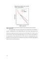
Figure 2.15: Neutrino mixing parameter space. In blue are the four islands of possible solutions to
the solar neutrino problem in 2000, LMA, SMA, LOW, and Vacuum; from the 2000 PDG [47].
26
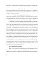
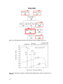
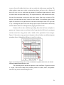
Figure 2.16: LMA solution. ∆m2 and tan2θ12 solutions to a Χ2 global fit to (a) the Chlorine, SAGE,
Gallex/GNO, Super Kamiokande, and SNO (D2O day and night spectra, salt CC, NC, ES fluxes)
experiments. (b) Previous result plus KAMLand results. [46]
Currently the best-fit point for ∆m122 and tan2θ12 with the new SNO data and
KAMLand results are:
•
∆m122 = 7.1+−10..26 × 10 −5 eV 2
•
θ 12 = 32.5 +−22..43 degrees
Future solar neutrino experiments will be able to either confirm the LMA solution and
put better limits on the mixing angle and mass differences or find something unexpected.
Atmospheric neutrinos put good limits on θ23 and with that we can have better knowledge
of θ13. Nevertheless, experiments dedicated to measuring θ13 will be able to provide a
result independent of θ23 and θ12.
The LMA solution is a matter enhanced oscillation effect, indicating that the
MSW effect is true. The MSW oscillations give us an effective Hamiltonian for twoneutrino mixing in matter:
 ∆m 2 cos 2θ
2G f ne
12

−

4 Eν
2
H =
∆m 2 sin 2θ 12


2 Eν


∆m 2 sin 2θ 12


2 Eν

2G f ne 
∆m 2 cos 2θ 12
+

4 Eν
2

The variables are the same as we have used previously. This Hamiltonian has both
a vacuum oscillation term and an MSW terms in it. To find which is more dominant at
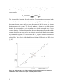
27
various energies, MSW or vacuum oscillations, a parameterization quantity, β, is defined
[48]. From the Hamiltonian above, we define β to be:
β =
2 2G f ne Eν
∆m 2
When we find the survival probability for the electron neutrinos, using the LMA
solution, we find that neutrinos will either oscillate more through the vacuum oscillation
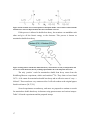
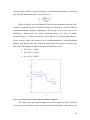
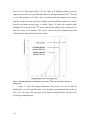
or matter dominated oscillations, depending on their energy. For β<cos2θ12 the survival
probability is dominated by the vacuum oscillation, where if β>1 then it is matter
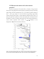
dominated. Figure 2.17 shows an example of this transition. For solar neutrinos there are
critical energies where the transition from vacuum-dominated to matter-dominated
happens. This depends on which reaction in the pp-chains the neutrinos are from in the
Sun, because they happen at different locations from the Sun’s center.
•
8
B-ν Æ E ≅ 1.8 MeV
•
7
Be-ν Æ E ≅ 2.2 MeV
•
pp-ν Æ E ≅ 3.2 MeV
Figure 2.17: Transition from Vacuum to Matter dominated oscillations.
The energy where the transition happens for the 8B-neutrinos is much lower than
we have spectral information about. Super Kamiokande, Kamiokande, and SNO rely on
28
the production of Čerenkov radiation, which gives them a threshold of about 5 MeV.
Such a high threshold makes the 8B-neutrinos measured to date matter dominated.
Measurements of lower energy neutrino spectrum will be able to give us insight into this
effect.
2.3.3 A 7Be-neutrino experiment: the next step
The solar neutrino experiments have been enormously successful in broadening
our knowledge of the neutrino. The possibility of neutrino oscillation was first observed
in solar neutrino experiments, beginning with Ray Davis’ Chlorine experiment. SNO’s
discrimination of the neutral and charged currents has shown that the number of 8B solar
neutrinos reaching the Earth are what we expect, and when included in a global fit with
the other experiments shows compelling evidence for LMA.
Although the circumstantial evidence is very strong, there is no smoking gun for
LMA. Additionally, the only spectral information we have of the solar neutrinos is above
~5 MeV, but this accounts for much less than 1% of the total solar neutrino flux.
Observation of the vacuum to matter dominated oscillation transitions would show strong
support for LMA and oscillations. Then a question arises: are there other effects at lower
energies that have not yet been seen?
Although a real-time measurement of the entire neutrino spectrum, including the
pp neutrinos, would be ideal, the technology for this measurement is still in the R&D
phase [49]. However, a real-time measurement of the 7Be neutrino is at hand. The 7Be
neutrino accounts for over 7% of the total solar neutrino flux and currently has the
greatest errors. Even with all the solar neutrino experiments and the reactor experiments
the 1σ uncertainty in the 7Be neutrino flux is still ±40%, and therefore demands a direct
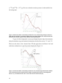
determination of its flux [50].
In addition to verification of the SSM, the 7Be neutrino flux will give us the first
insight into the luminosity constraint. If Hans Bethe’s prediction for energy production in
the Sun is correct, then the energy emitted by photons should correlate with that emitted
by neutrinos. This constraint is used very often in analysis of the solar neutrinos, but it
has never been experimentally proven. A 7Be neutrino experiment will give us the first
true insight into this, but only a measurement of the pp neutrinos can prove the
29
luminosity constraint. If it proves to be false, then there are either other energy
production mechanisms in the Sun, or the steady state assumption for the Sun may be
incorrect.
30
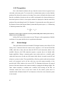
Chapter 3:
The Borexino detector
Borexino is a solar neutrino detector designed to measure the flux of the so called
7
Be neutrino produced in the core of the Sun. By measuring this flux one obtains initial
insights into the energy spectrum of neutrinos below the current lower limits set by
Super-Kamiokande [10] and the Sudbury Neutrino Observatory (SNO) [11], which have
a lower limit near 5 MeV. Better limits will also be placed on the mixing parameters in
the solar neutrino sector, namely θ12 and ∆m122, which provides an independent
verification of the Large Mixing Angle (LMA) solution in the mixing parameter space.
The measurement will be the next step towards understanding the luminosity constraint,
which limits the energy emitted by solar neutrinos by the energy emitted by photons. A
violation of the luminosity constraint could provide motivation to consider such things as
new energy production mechanisms or perhaps the Sun is not in a steady state as we
expected, which was detailed more in the pervious chapter. If the LMA solution to
neutrino oscillations is true then an interesting phenomenon arises whereby the low
energy neutrino will oscillate predominately through the vacuum oscillation rather than
through matter-enhanced oscillations.
3.1
Borexino design
Borexino is a liquid scintillator detector designed to measure the neutrino-electron
scattering of mono-energetic 7Be neutrinos. Neutrino-electron scattering does not have a
unique signature so in the end we will have to extract the 7Be neutrino flux from the
background produced by radioactive contamination both internal and external to the
detector. The mono-energetic nature of the 7Be-neutrinos means that they will leave a
Compton-like edge in the spectrum due to the recoiling electron in neutrino-electron
elastic scattering. This Compton-like edge has a maximum value of 660 keV [17];
however, the background within the neutrino window imposed by the detector
configuration (250 keV to 800 keV) needs to be low enough to recognize this effect.
31
The basic detector concept is quite simple; it is a scintillator viewed by
photomultiplier tubes (PMT). The scintillator produces light when it is excited through
collisional excitation or ionization by the recoil electron from neutrino-electron
scattering, and the PMTs measure this light. The amount of light produced is proportional
to the energy deposited in the scintillator. Since alphas, betas and gammas can excite the
scintillator, as well as neutrinos, they become the major background, and the overall
design of the detector is driven by the reduction of events that yield these particles. The
external backgrounds, primarily gammas from the detector materials and other sources
outside the detector, dictate the amount of shielding needed throughout the detector, and
the intrinsic radioactive contamination of the scintillator requires an efficient purification
system.
3.1.1 External backgrounds
Solar neutrinos arrive at the Earth at a rate of approximately 65 billion per cm2
per second, but since the neutrino-electron scattering cross-section is on the order of 10-44
cm2 only a very few of them will ever interact in the Earth let alone in a detector. On the
other hand, cosmic rays, which include deeply penetrating muons, although not as
plentiful as neutrinos, do interact quite readily and become the dominant background in
neutrino detectors that are positioned at the surface. To suppress this background,
Borexino is placed approximately 1 mile underground in the Istituto Nazionale di Fisica
Nuclaere’s (INFN) Laboratori Nazionali del Gran Sasso (LNGS) located east of Rome in
Italy’s Abruzzo region. This overburden eliminates all the cosmic rays except for a
portion of the muons whose flux is reduced by a factor of one million, down to about 1
muon per square meter per hour.
The problem now becomes the radioactivity from the surrounding rock, namely
the gamma emitters, which can penetrate deep into the detector. These are eliminated
with a water shield, which is over 2 meters thick. Borexino’s water shield is an 18 meter
diameter water tank, concentric to the stainless steel sphere (SSS) that houses the detector
material/target. A drawing of the Borexino detector is displayed in Figure 3.1, and will be
referenced throughout the description of Borexino’s design.
32
Figure 3.1: BOREXINO design.
A Stainless Steel Sphere (SSS) 13.7 meters in diameter lies concentric to the
water-tank, and is the mounting point for 2214 PMTs, 1800 of which have light
concentrators to increase the light collection efficiency. At this point the gammas from
the rock have been blocked, but now the radioactivity of the building materials
themselves becomes a problem. Gamma emitters from the SSS and PMTs could reach the
inner detector, and therefore the detector is self shielded. This means that we use a buffer
liquid between the SSS and the scintillator to block the gammas from the construction
materials. A clear nylon vessel, 8.5 meters in diameter, concentric to the SSS, contains
300 tons of active liquid scintillator. The active scintillator is produced by mixing a fluor
33
and a solvent; where as the buffer liquid is made of the scintillator solvent and a quencher
(dimethylphtalate), which does not scintillate. This reduces the amount of strength the
nylon vessel needs to have against any buoyant force, thereby making it as thin as
possible.
This vessel is called the inner-vessel (IV), because in addition to this there is an
outer-vessel (OV) with an 11.5 meter diameter. The OV is used to block the propagation
of
222
Rn released by the various detector materials due to
226
Ra contamination; for this
reason the OV is also called the “Radon Barrier”. Radon can diffuse through the nylon
vessel and can therefore enter the IV. Radon emanation happens because 226Ra is a solid
that decays into the gaseous
222
Rn, which is then emanated from the material. All the
materials in the detector are tested for their radon emanation as well as contamination
from gamma emitters, which are of concern to Borexino [51].
To further reduce the background from gammas emitted by the detector materials,
including the nylon vessels and radioactive contamination on their surface, a data taking
region is defined in space. This trustworthy or “fiducial” volume contains 100 tons of
liquid scintillator and is approximately 6 meters in diameter. This method requires
precise determination of the event position so that if it falls outside of the fiducial volume
it can be eliminated from the data sample. This final shielding reduces the number of
background events due to external gammas from approximately 5000 events per day, if
the entire IV where used, to much less than 1 per day when a 100 ton fiducial volume is
used [52].
3.1.2 Internal backgrounds
The mountain, the water-tank, the outer buffer (between the SSS and OV), the
inner buffer (between the OV and IV), and the fiducial volume cut all form an onion skin
type shielding where each progressive layer shields from the previous. This approach
nearly eliminates external backgrounds from the data. What remains are the intrinsic
backgrounds due to radioactive contamination in the scintillator itself. These
backgrounds include alpha, beta, and gamma emitters, whose energies fall within the
neutrino window. The alphas are a special case because their light yield is only 10% that
of a similar energy beta.
34
Three types of natural radioactivity are especially bothersome because they have
emissions in the energy window for 7Be neutrino detection. They are:
•
Primordial radioactivity: 40K, and the 238U and 232Th decay chains
•
Noble gases: 222Rn and 85Kr (from atmospheric nuclear weapons testing)
•
Cosmogenic activities: 14C and 7Be
The
14
C is particularly dangerous because the scintillator is based on an organic
solvent (pseudocumene), made almost entirely of carbon. Although the end point of the
14
C beta spectrum is 156 keV it tails into the neutrino window due to limited energy
resolution and pile-up, and for this reason Borexino requires
14
C/12C ≈ 10-18 g/g. It is
reduced by using pseudocumene produced from crude oil, where the natural
decayed away. The only
14
14
C has all
C in the pseudocumene is produced through cosmogenics
during its time on the surface of the Earth, and activation from the radioactivity in the
rock of the oilfield. The 7Be is also minimized by limiting the time the pseudocumene is
not underground.
The other activities are different from the
14
C in that they can be removed from
the scintillator, because they are not an inherent part of the pseudocumene. However,
until Borexino the purity requirements (K ≈ 10-14g/g, U/Th ≈ 10-16g/g) had not been
achieved on a multi-ton scale. To remove the metallic and gaseous contaminants several
methods are employed: vacuum distillation, water extraction, filtration, and nitrogen
stripping [53]. To measure this purity level, and to verify the purification techniques, a
prototype of Borexino named The Counting Test Facility (CTF), was constructed. The
CTF will be described in more detail later in this chapter.
With the radioactivity at the lowest levels possible the question may arise: is this
low enough? Can we extract the 7Be-neutrino flux measurement out of the background
produced by the internal activity still left in the detector? The answer is no. The expected
neutrino rate in Borexino is on the order of tens of neutrino events per day. If we assume
a purity level of 10-16 g/g for 238U and 232Th and 10-14 for natural K then the total number
of background events in the neutrino window in the fiducial volume is 122 events per
day, several times greater than the neutrino rate in the fiducial volume. To have a signal
to noise ratio near 3:1 we still need to remove the background events by tagging them.
35
3.2
The scintillator
Scintillator is a material which is transparent to the light produced within it when
excited. In Borexino this scintillator is a cocktail of 1,2,4 trimethylbenzene or
pseudocumene (PC) as the main solvent and 2,5 diphenyl oxazole (PPO) as a fluor at a
concentration of 1.5 g/l. When excited, the scintillator will emit light in a narrow band of
wavelengths. The PPO in Borexino’s scintillator acts as a wavelength shifter, or fluor,
which shifts the wavelength (Stoke’s shift) of the emitted light to a longer wavelength
than the emitted light of pure PC. This happens through non-radiative transfer to lower
energy states, which will make the scintillator more transparent to its own light, but also
matches the quantum efficiency of the PMTs. Figure 3.2 shows how the PPO shifts the
wavelength of the emitted light and how well that matches the quantum efficiency of the
PMTs.
Figure 3.2: Emission spectra and PMT quantum efficiency. By mixing PPO in with the PC the final
cocktail becomes more transparent to its own light, which matches the quantum efficiency of the
PMTs very well.
When a charged particle excites the PC it creates excited π-electrons, and when
they decay down to the ground state they produce scintillation light. The PPO is at such a
36
small concentration that its direct excitation is negligible. There are also other excitations
in the molecules, but these do not lead to scintillation light and therefore are not
considered. However this has the effect that the energy deposited in the scintillator will
not match that emitted as scintillation light; generally only 5% of the deposited energy is
emitted in detectable light.
Figure 3.3 shows the energy levels of the singlet and triplet states of a scintillator.
Excitations into the singlet states are primarily collisional excitations, where transitions to
the triplet states are possible through ion-recombination or intersystem crossing. The
intersystem crossing is a spin-orbit coupling that allows an electron to cross between the
singlet and triplet states. These triplet states may decay radiatively through
phosphorescence with lifetimes on the order of 100µs, which is a very long lifetime, and
therefore does not contribute to the scintillation light collected in the time window of the
detector.
Figure 3.3: Energy levels for π-electrons in the scintillator [52]. Only charged particles are able to
excite the scintillator into the triplet states, and therefore only α and β calibration sources can be
used to probe this effect.
Massive charged particles are able to ionize the scintillator, and therefore the
number of triplet state excitations due to ion-recombination is ionization density
dependent. Therefore the longer lived ionization-recombination triplet state excitations
37
are more favored by alphas than betas, and can explain the alpha energy quenching. The
alpha produces many more triplet excitations than betas, and since only a fraction of
these will cross over to a singlet state the amount of scintillation light produced is much
less than a beta with equivalent energy. The singlet states decay with characteristic times,
but since the intersystem crossing also takes time, energy from these excitation will be
delayed. An alpha and beta may create the same amount of scintillation light, but the
alpha will emit more of its light later due to the extra excited triplet states. This gives one
a way to distinguish alphas from betas through pulse shape discrimination, and thereby
facilitate further reduction of background by tagging unwanted events.
Gammas will also have a different quenching factor than the betas and alphas. A
gamma can Compton scatter several times before being absorbed, effectively creating not
one but several low energy betas each of which will be quenched at lower energies.
Figure 3.4 shows the energy spectrum of gammas with and without an additional gamma
quenching factor. Although the difference is small it is evident.
Figure 3.4: Gamma quenching. These results are simulations of gammas in Borexino, run with and
without an additional quenching factor [52].
The quenching factors depend on impurities in the scintillator. Of greatest concern
is oxygen, which could change the quenching factors for alphas, betas, and gammas.
Therefore they must be understood quite well.
38
3.3
Background subtraction
Having different pulse shapes for alphas and betas, Figure 3.5, gives us a method
for tagging alpha events through pulse shape discrimination. We can also look for
decayed coincidences in the U and Th chains, which can then be used to statistically
subtract other background events.
Figure 3.5: Photon time distribution. This graph shows scintillation light pulses for 750 keV betas
and alphas whose emitted energy has been quenched to 750 keV. This data comes from Monte Carlo
of the Borexino detector. All the events are from the center of the detector. The shapes are different
enough to be able to distinguish them in Borexino so that the alphas events can be removed.
3.3.1 Pulse Shape Discrimination
Borexino measures the recoiling electron in neutrino-electron scattering. This will
produce the same scintillation pulse shape as a beta, but since alphas have a different
shape we can cut them out of the data by pulse shape discrimination. A simple method
for alpha/beta separation is the tail-to-total ratio. In this method the tail of the pulse after
a characteristic time threshold is integrated and divided by the total integrated pulse.
Since alpha pulses have a longer tail, they will have a higher ratio than an equivalent
beta. Figure 3.6 shows a histogram of the tail to total ratio for alphas and betas with
equivalent energies. The crucial part is the amount of overlap between the alphas and
betas. The neutrino events appear as betas, so we want to keep as many betas events
while minimizing the number of residual alphas kept in the analysis. Figure 3.7 shows a
graph of the tail/total ratio versus energy in the CTF. Visually we can see that the higher
39
energy events are well separated, but the lower energy events are not, and this effect will
lead to more alpha events bleeding into the final beta energy spectrum to be fit. One
major question is whether performing position dependant alpha/beta separation will
significantly reduce the residual alphas.
Figure 3.6: Sample Tail/Total ratio histogram. This histogram was created from Monte Carlo data of
the tail to total ratio for alpha and beta events from the center of Borexino. The data used in this
histogram is the same as in Figure 3.5. The overlap of the histograms causes some alphas to be tagged
as betas and some betas to be tagged as alphas.
Figure 3.7: Tail to Total ratio from the CTF [54]. The higher ratios are from alphas, because of their
longer tails. The energy dependence means that there are more alphas at lower energy incorrectly
tagged as betas than at higher energies.
40
3.3.2 Delayed coincidence and Statistical subtraction
In the Uranium and Thorium chains, Figure 3.8, there are two isotopes that decay
close enough in time so that they can be tagged due to this characteristic time. In the 238U
chain
214
Bi will beta decay into
214
Po which alpha decays later with a lifetime of 164µs.
Likewise, in the 232Th chain a fraction of the 212Bi beta decays into 212Po and then it alpha
decays with a 299ns lifetime.
Figure 3.8: The 238U and 232Th chains. These chains are the major part of the background in
Borexino; however there is a delayed coincidence in each chain between Bismuth and Polonium.
When the Bi-Po coincidences have been found, then it is possible to say
something about the rest of the chains. We know what the rest of the chains look like, and
they must come later once we have tagged the Bi-Po. If we assume secular equilibrium
then we can also calculate how many of the previous decay products in the chains should
have been in the data before the Bi-Po. This technique has limitations due to the very
long lifetimes of some of the parents, but right before the Bi-Po there are several parents
with lifetimes on the order of minutes. By using a Monte Carlo to determine their spectra
we can statistically subtract them from the overall spectrum.
A delayed coincidence also exists for
85
Kr, which has a 0.43% chance of beta
decaying into a metastable state of Rubidium (85mRb), which gamma decays to its ground
state. The lifetime of
41
85m
Rb is 1.46µs, which makes it a great candidate for delayed
coincidence. For every one of these tagged events there will be ~231.5 normal 85Kr beta
events [55].
3.4
The Counting Test Facility (CTF)
The CTF was built in order to test whether it is possible to produce a scintillator
pure enough for Borexino, and to show that event tagging and removal would work,
thereby allowing Borexino to determine the 7Be-neutrino flux. It is effectively a miniBorexino, but there are some pronounced differences. The CTF uses an inner vessel with
a two meter diameter, which contains nearly 4 tons of the PC/PPO scintillator. As a
buffer/shielding liquid the CTF uses water in an 11m tall, 10 m diameter cylindrical tank,
and because of the differences in density there is a strong buoyant force that requires a
thicker nylon film. The original CTF did not have a radon barrier, but in 2000 a new set
of vessels were installed, which included an outer vessel to decrease the number of radon
events in the IV. The shielding in CTF is not as great as Borexino, but the CTF was not a
singles experiment like Borexino but rather a coincidence experiment searching for the
Bi-Po coincidences in the
238
U and
232
Th chains to prove that they could be removed to
the levels Borexino requires. The IV is viewed by 100 PMTs all of which have light
concentrators, and are mounted to a structure made from stainless steel tubing rather than
a sealed sphere like Borexino. Figure 3.9 shows a picture of the interior of the original
CTF without the OV.
42
Figure 3.9: Original CTF. Unlike Borexino the PMT are supported by an open structure. This photo
does not have the radon barrier, which now exists in the CTF.
The CTF detector was able to show that the scintillator purity levels sought by
Borexino were achievable with purification, and that the alpha/beta separation technique
could sufficiently reduce the remaining backgrounds. The purity levels achieved were:
•
14
C/12C = (1.94±0.09) × 10-18 g/g
•
232
Th = (4.4+1.5-1.2) × 10-16 g/g
•
238
U = (3.5±1.3) × 10-16 g/g
which are not good enough, but Borexino has a better surface to volume ratio than the
CTF and therefore we hope that there will be fewer internal contaminates.
43
After the prototype phase, CTF was to be used as a screen to measure the
14
C
content of the scintillator, so that pseudocumene with large amounts of 14C are not used
in Borexino. However the CTF has also been used to study whether any of the fluid
handling systems contaminate the scintillator with radio-impurities or contaminates
which may affect the quenching factors. Since it has been running for so long, it has also
been very fruitful in putting several limits on physics, some of which have been included
in the 2004 Particle Data Book. For example:
3.5
•
“Search for neutrino radiative decay with a prototype Borexino detector.” Derbin A.,
Smirnov O. JETP Lett. Vol 76, No 7 (2002) 409-413.
•
“Search for electron decay mode e → γ + ν with prototype of Borexino detector.” H. O.
Back et al. Physics Letters B 525 (2002) 29. {PDG 2004}
•
“New limits on nucleon decays into invisible channels with the BOREXINO Counting
Test Facility.” H. O. Back et al. Physics Letters B 563 (2003) 23. {PDG 2004}
•
“Study of the neutrino electromagnetic properties with the Prototype of the Borexino
Detector.” H. O. Back et al. Physics Letters B 563 (2003) 37. {PDG 2004}
•
“New experimental limits on heavy neutrino mixing in B-8 decay obtained with the
Prototype of the Borexino Detector.” H. O. Back et al. JETP Lett. Vol 78, No 5 (2003)
261-266.
Borexino expected performance
Since Borexino measures the neutrino through neutrino-electron scattering, and
not by neutrino absorption, the neutrino will only deposit a fraction of its energy in the
scintillator. This will produce a Compton-like edge in its energy spectrum, with a
maximum energy at
Tmax =
Eν
m
1+ e
2 Eν
where Eν is the energy of the neutrino. The neutrino energy spectrum is then hidden
under all the background. Shielding and purification are able to eliminate nearly all the
backgrounds; but if the LMA solution is correct then Borexino will only see
approximately 25 7Be-neutrinos per day [17]. The expected signal from Borexino, if the
neutrinos were not changing flavor, is presented in Figure 3.10. The background assumed
44
is 238U and 232Th ~ 10-16 g/g. We can see that the neutrino spectrum is indiscernible from
the background.
Figure 3.10: Borexino Monte Carlo fitted spectrum before cuts. All the backgrounds present before
PSD, delayed coincidence, and statistical subtraction cuts and the standard solar model neutrino flux
prediction. The neutrino signal is clearly buried in the background [52].
To get rid of the background we must go through the pulse shape discrimination,
delayed coincidence tag, and a statistical subtraction described in sections 3.3.1 and 3.3.2.
When we take what we have learned from CTF and apply that to the Monte Carlo and
make these subtractions we get the spectrum displayed in Figure 3.11.
Figure 3.11: Borexino Monte Carlo fitted spectrum after cuts. All the backgrounds and the standard
solar model neutrino flux prediction after the all the cuts mentioned in the text. The background
must be very well understood in order to extract the total 7Be neutrino flux [52].
45
In this spectrum the “shoulder” that is produced by the 7Be-neutrinos is much
more pronounced, however we must remember that it appears that the LMA oscillation
solution to solar neutrino deficit appears to be correct, and that Borexino will only detect
approximately 50% of the neutrino flux because the neutrinos have changed flavor.
Neutrino-electron scattering occurs with all flavors of neutrinos, but because the electron
neutrino can interact through both the neutral and charged currents Borexino is much
more sensitive to them. The neutral current cross section is approximately 1/5 that of the
charged current cross section. Therefore in Borexino the neutrino energy spectrum will
be about 50% of that shown in Figure 3.10 and Figure 3.11.
There are several points to keep in mind when studying Figure 3.10 and Figure
3.11. Neutrinos, because of the scattering, act like betas in Borexino, but this has a
different quenching factor than the alphas, and thereby the absolute energy scales of the
alphas and betas are different. In order for us to accurately predict the backgrounds and
thereby make a fit to the spectrum, we must know the energy scales and the shape of the
background spectrum very well. The predicted shape of the background, which will in the
end be fit to Borexino’s spectrum, is dependent on the knowledge of the alpha/beta
separation efficiency as a function of energy. If there is an unknown energy dependence,
then the background will be fit incorrectly, thereby lowering the accuracy of the extracted
7
Be-ν flux. Figure 3.12 shows an extreme example where the actual residual 232Th alphas
suddenly decrease due to better alpha/beta separation efficiency above a certain energy
threshold. Although extreme, this shows that if the energy dependences are not properly
taken into account then the final fit may be incorrect. Therefore the alpha/beta separation
efficiency must be well understood throughout the detector and over the energy window
of the detector.
46
Figure 3.12: Hypothetical spectrum with poor alpha/beta separation. If the actual 232Th spectrum is
much different from the predicted spectrum, then the final fit will be incorrect, and the accuracy in
the extracted 7Be-ν flux will decrease.
The Monte Carlos are also run with a known fiducial volume cut, however in the
final geometry we will need to measure the accuracy for defining the fiducial volume.
The only signature in Borexino for the solar nature of the 7Be-neutrino is the 7% change
in the flux due to the eccentricity of the Earth’s orbit. The fiducial volume needs to be
known well enough to measure this effect. Any error in the fiducial volume leads to an
error in the absolute flux Borexino will measure. Every centimeter error in the fiducial
volume radius, assuming a 300 cm radius, equates to a 1% error in the neutrino flux.
3
∆r ∆V
=
r
V
∴ ∆V = %1 ⇒ ∆r = 1cm
In order to learn as much as we can about the detector, so that a high precision
measurement of the 7Be-neutrino flux can be extracted, we must carefully calibrate the
detector. The absolute energy scales must be known accurately as well as the alpha/beta
separation efficiency, and thereby the delayed coincidence tags and our statistical
subtraction ability must also be found. Other unknown position dependencies in the same
quantities may also exist. All of this can be measured if known radioactive calibration
sources are positioned accurately throughout the detector, which is the basis for the rest
of this dissertation.
47
Chapter 4:
Internal source calibration
In order to understand Borexino and to extract the most precise measurement of
7
the Be-neutino flux from the Sun, a rigorous calibration of the Borexino detector must
take place. The separate energy scales of alphas, betas, and gammas must be known, and
the efficiencies for tagging alphas and betas needs to be maximized and known.
To extract the 7Be-neutino flux from the output spectrum of Borexino we need to
perform a combined fit of the various backgrounds and the shape of the recoil electron
spectrum from the 7Be-neutino. Such a fitting routine assumes we know the basic shape
of the background spectra for the various isotopes and the neutrino spectrum, and must
account for any alpha/beta separation energy dependence. Any unforeseen energy
dependence will decrease the precision of the final determination of the 7Be-neutino flux,
and thereby the confidence level of Borexino measurement.
Borexino will likely have a density of radioactive contaminants as described in
chapter 3, and they can be used for some of the calibration if they can be identified
accurately. It is also possible to study some of the scintillation properties through
excitation by ultraviolet light. UV lasers can study scattering and absorption through the
inner vessel scintillator and other laser sources can study scattering and absorption in the
buffer liquid. There are also laser sources that are able to excite π-electrons up to their
singlet states, where the scintillation light comes from. However the lasers are not able to
study the longer lived part of the scintillation pulse; only massive charged particles can
fully ionize the scintillator into triplet states, which contain the information about particle
identification (section 3.2). Chapter 7 details some of the ultraviolet laser calibration
systems, but a more rigorous discussion of these systems can be found in [52].
Borexino’s expected final spectra after the alpha/beta separation, delayed
coincidence and statistical subtraction cuts, shown in the previous chapter in Figure 3.11,
assumes a purity of the scintillator about a factor of five better than what was found in the
CTF. If in Borexino a better purity is not achieved then event tagging will become even
more important. For example if there is much more
232
Th than assumed, then the low
48
energy “hump” will be larger and the 7Be-neutrino shoulder may be lost in the tail of this
background. To overcome this possible effect, alpha/beta separation must be optimized,
which must include any spatial or energy dependences that exist.
For the most complete understanding of the detector’s alpha, beta, and gamma
energy scales and particle tagging efficiencies, calibration sources that emit alphas, betas,
and gammas of various energies must be used.
4.1
PSD spatial dependence
A Monte Carlo was run to study the possible spatial dependencies on alpha/beta
separation efficiency in Borexino due to known anisotropies in its geometry and
scintillator effects. If such a spatial dependence does exist in this simulation then there
may be additional unknown non-uniformities which could effect the overall extraction of
the 7Be neutrino flux. The only way to determine the alpha/beta separation throughout the
detector is with radioactive calibration sources.
Borexino is not perfectly spherically symmetric in its light collection efficiency.
The vessels are mounted to the top and bottom poles of the SSS with a support structure,
which displace some PMTs and can block the light from events. There is also a 3 meter
port near the bottom of the SSS used for access during detector assembly. This port is not
flush with the rest of the SSS when closed and therefore the PMTs on it lie several
centimeters further from the center of the detector; more significant than the distance
from the center is that there are missing PMTs due to the structure of the port, which
decreases the light collection efficiency is this area of the detector. The legs of the SSS
also prevent installation of several PMTs on the lower hemisphere near the equator.
Figure 4.1 shows a map of the holes in the SSS, where you can see the missing PMTs,
which are crossed out.
In addition to the light collection anisotropies there are other phenomena which
affect the propagation of light in the detector. Light scattering and absorption in the
scintillator should not be position dependent, but they are photon path length dependent
[56]. The further from the center of the detector an event occurs, the closer it will be to
PMTs on one side of the detector and the further it will be from others. This changes the
amount of time photons spend in the detector.
49
Reflections will also have an effect on the alpha/beta separation efficiency. Light
reflected off of the SSS, the PMT light collector, or the PMT photocathode will travel
even further in the scintillator, and will be delayed by its time of flight (10’s of
nanoseconds). These photons are indiscernible from the non-reflected photons. Therefore
they will show up at a later time in the pulse, and can only be taken into account through
simulation. The tail of the pulse is where the information about particle identification
resides, and these reflections may therefore influence the particle identification.
Figure 4.1: Layout of holes on Borexino SSS. Missing PMTs are marked by X’s.
4.1.1 The Monte Carlo
The Fortran tracking code of the Borexino Monte Carlo simulation developed at
the INFN in Milan was run to conduct the alpha/beta spatial dependency study. Figure
4.2 shows the global structure of the Borexino event generation and reconstruction. In our
simulation we replaced the full event generator code, GENEB [57], by inputting 450 keV
and 750 keV betas, and alphas with equivalent beta energies placed at several points
throughout the detector. The photons produced in these events are tracked through the
detector until they reach a PMT photocathode, where a photoelectron may be created
depending on the quantum efficiency of the PMT.
50
The simulation event coordinates effectively map out four lines in the detector:
from the center toward the top of the SSS, from the center to the bottom of the SSS, from
the center toward the 3 m port (which points 60º below the SSS equator toward north),
and from the center to the east which is orthogonal to all the other lines. Table 4.1 lists all
the points and their coordinates, where the center of the SSS is the origin, the z-axis is
vertical, the x-axis points south, and the y-axis points east. The theta and phi coordinates
are measured from the x-axis (south).
Figure 4.2: Borexino global code structure.
51
x
(meters)
y
(meters)
z
(meters)
1
2
3
4
5
6
7
8
9
10
11
12
13
14
15
16
17
18
19
20
21
22
23
24
25
26
27
28
29
30
31
32
33
4.0
3.5
3.0
2.5
2.0
1.5
1.0
0.5
0.0
0.5
1.0
1.5
2.0
2.5
3.0
3.5
4.0
0.5
1.0
1.5
2.0
2.5
3.0
3.5
4.0
0.5
1.0
1.5
2.0
2.5
3.0
3.5
4.0
-90
-90
-90
-90
-90
-90
-90
-90
-90
90
90
90
90
90
90
90
90
-60
-60
-60
-60
-60
-60
-60
-60
0
0
0
0
0
0
0
0
0
0
0
0
0
0
0
0
0
0
0
0
0
0
0
0
0
180
180
180
180
180
180
180
180
90
90
90
90
90
90
90
90
0
0
0
0
0
0
0
0
0
0
0
0
0
0
0
0
0
-0.25
-0.50
-0.75
-1.00
-1.25
-1.50
-1.75
-2.00
0
0
0
0
0
0
0
0
0
0
0
0
0
0
0
0
0
0
0
0
0
0
0
0
0
0
0
0
0
0
0
0
0
0.5
1.0
1.5
2.0
2.5
3.0
3.5
4.0
-4.0
-3.5
-3.0
-2.5
-2.0
-1.5
-1.0
-0.5
0
0.5
1.0
1.5
2.0
2.5
3.0
3.5
4.0
-0.433
-0.866
-1.299
-1.732
-2.165
-2.598
-3.031
-3.464
0
0
0
0
0
0
0
0
Line in
SSS
Center
Center toward east
Phi
(degrees)
Center toward 3m
port
Theta
(degrees)
Center toward top
R
(meters)
Center toward
bottom
Point
Table 4.1: Simulation source coordinates. The coordinate origin is the center of the SSS and
The simulation takes into account all scintillation effects such as absorption,
scattering, and scintillation light production processes. It also includes reflections from
the SSS, but not reflections from other sources in the detector. It also does not include
some detector infrastructure such as the mounting support for the vessels. The missing
vessel end regions mean that effects due to the light normally blocked by them will not be
included. Our study will show that there are spatial and energy dependences with a
simple Monte Carlo.
In our study, we only wanted to look at the raw output of the detector so that any
electronic or reconstruction effects would be removed. Our reconstruction takes into
account the known position of the event, the time of the event, and the time of each
photoelectron detected in an event. The time of flight for each photoelectron in an event
is subtracted from the detection time of that photoelectron. Since we know where the
event took place and the coordinates of the PMTs which detected the photoelectron, then
52
we can find the unscattered path length for the photon. Knowing that the index of
refraction for the scintillator is 1.5 makes it trivial to find the time of flight. However, this
time of flight calculation cannot distinguish direct photons from photons reflected off the
SSS, which means that a time of flight ambiguity. This scenario is the same as in the final
Borexino.
The time of the first detected photon, after the time of flight correction, is found
and subtracted from the corrected times of the remaining photons in the event. This will
give us the final time distribution of photons for a single event, where the first photon is
detected at time t = 0, which assumes a perfect trigger. The time distribution of the
accumulative events of the simulation at the center of the detector was shown in the
previous chapter, Figure 3.5.
In our analysis we use the tail to total ratio method for alpha/beta discrimination.
The number of photoelectrons arriving after a set time threshold are divide by the total
number of photoelectrons in that event. Since the alphas have longer tails they will have a
higher ratio than the betas; thereby making them differentiable. In our analysis we used a
time threshold of 25 ns for the tail/total ratio, which was found to be the best for the
Borexino scintillator in reference [58].
4.1.2 Alpha/beta separation spatial dependence
The neutrino-electron scattering in Borexino is indistinguishable from beta decay
and therefore the main objective of the pulse shape discrimination is to keep as many beta
events while minimizing the number of alphas events. Figure 4.3 shows the tail/total ratio
for 450 keV events at the center of the detector. While the alpha and beta events are
nearly separated, there is an overlap, which will lead to a bleed-through of alpha events
into the beta spectrum. In Figure 4.4 we can see that the higher energy events have a
smaller overlap, and are therefore better separated. Figure 4.5 shows a contour plot of the
tail/total ratio for both 450 keV and 750 keV alphas and betas. From these figures we can
start to see an energy dependence in the alpha/beta separation. We now need to define a
cut ratio where events with lower ratios will be kept as beta events, while the higher
ratios are discarded as alphas.
53
Figure 4.3: Alpha/beta separation with 25ns time threshold for tail for 450 keV events.
Figure 4.4: Alpha/beta separation with 25ns time threshold for tail for 750 keV events. Visually this
is more separated than the 450 keV events.
54
Figure 4.5: Contour plot of tail/total ratio versus total number of photoelectrons for both 450 and 750
keV events.
To make our comparison of alpha/beta separation versus position we make our
ratio cut at the point were we only loose 5% of the betas. This ratio threshold is found by
fitting a Gaussian to the beta tail/total ratio histogram and finding the ratio where 5% of
the betas are in the tail that overlaps the alphas. In Figure 4.3 that ratio is equal to ~0.41,
where for the 750 keV events, Figure 4.4, that ratio is ~0.40. This “optimum” threshold
ratio was found for every position in the simulations and plotted as a function of radius
for both 450 keV, Figure 4.6, and 750 keV, Figure 4.7. We can see that there is a strong
radial dependence, which changes the ratio by nearly 10% from the center out to 4
meters. The fiducial volume stops at 3 meters, but there is still nearly a 5% difference
between there and the center. We can also see a slight difference between the two
energies, however there is not much difference between points at the same radii.
55
Figure 4.6: Threshold ratio to tag 95% of the betas versus radius (for 450 keV events).
Figure 4.7: Threshold ratio to tag 95% of the betas versus radius (for 750 keV events).
If we now take these optimum cut ratios found for each position and integrate the
alpha tail/total ratio histogram below that point, then we can find how many residual
alphas are left in the beta spectrum at each point. In Figure 4.8 and Figure 4.9 we see
again a strong radial dependence where the alpha/beta separation efficiency is greater the
56
further we go from the center of the detector. We can start to see a difference in the
number of residual alphas at the points at the same radius from the center. The most
striking difference we see is the energy dependence. The higher energy events are far
better separated than the lower energy events.
Figure 4.8: Ratio of residual alphas to total alphas versus radius (450 keV).
Figure 4.9: Ratio of residual alphas to total alphas versus radius (750 keV).
57
4.1.3 Conclusion
The alpha/beta separation has an obvious spatial dependence in even our simple
separation technique (tail/total ratio). Although the spatial dependencies we find are
primarily a function of radius, we do see the beginnings of efficiency differences as a
function of azimuthal and polar angles. The radial dependence we have found is due to
very well known scintillator effects and geometries of Borexino, and does not take into
consideration several other known non-uniformities, let alone any unknown ones (for
example scattering in the vessel film, light blockage due to the seams on the vessel, etc.).
The most striking difference in the separation efficiencies is between the two energies. At
lower energies the alpha/beta discrimination is not as efficient as at higher energies and
causes the “hump” in the expected Borexino spectrum after the various cuts are made, as
shown in Figure 3.11 in section 3.5.
It can be argued that we can use the intrinsic radioactive contamination to study
the alpha/beta separation, but this requires a good understanding of detector effects and
the spectrum of the events (whether the U and Th chains are in secular equilibrium or
not). At 122 background events per day the statistics do not allow spatial dependence
studies. This background rate is approximately one event per ton per day, which means
that we would need a very long time if we wanted to study per ton effects (3 years to get
1000 background events per ton).
By using radioactive calibration sources of various energies and particle types
throughout the detector we can find the optimum alpha/beta separation efficiency for the
detector as a whole. Added non-uniformities may further separate the number of residual
alphas in the beta spectrum as a function of position, which further strengthens the case
for radioactive source calibration. These sources can also be used to do an energy
calibration for alphas, betas, and gammas, without having to fit to the spectrum of
background events.
4.2
Method
A 100% effective calibration source would mimic the natural radioactivity
exactly. However the isotopes need to be contained and they need a support structure. All
of which may distort the energy deposited in the scintillator or the light output of the
58
scintillator. The design of the calibration sources minimizes the light blockage and
maximizes the energy deposition of the energy from the alphas or betas.
To have effective sources we would like to have statistically significant data at
several positions in the detector, and have it all done in a reasonable amount of time.
However this must be balanced by the risk to the detector. If a source isotope is released
into the detector then the background may increase significantly. However if we use a
short lived source then we can wait for it to decay away, if an accident were to occur. If a
long lived source must be used, then it should be removable by Borexino’s scintillator
purification system. Currently the sources have 10-100 Bq of activity, which will give us
a 1% rate measurement after less than a quarter of an hour. The design of the source
minimizes the risk to the detector by making them completely sealed, and by having an
insertion system (chapter 5) that prevents the source from dropping into the detector.
4.2.1 Design
The overall design of the sources is the same. A one inch in diameter quartz vial
is loaded with scintillator in which the source material is suspended, Figure 4.10. The
quartz is fused to a metal tube, which is crimped shut so that the source will not leak.
Such a crimp was leak checked to better than 10-10 mbar/liter/second, which means that
the radioactive material within the vial cannot escape.
Figure 4.10: Calibration source quartz vial.
In order to make sure that the calibration sources act as much like alpha and beta
events in Borexino they must meet several requirements.
59
•
To minimize the light blockage due to the neck of the vial, its diameter
will need to be as small as possible. In the current design the neck blocks
less than one percent of the light emitted in the vial.
•
The energy calibration and pulse shape discrimination efficiency are
functions of the scintillator, and therefore the calibration source needs to
use the scintillator from the detector.
•
The number of events that can interact with the vial surface must be
minimized. This will distort the average energy spectrum of the source.
To use the scintillator from the detector, we must pass it from the detector to the
source vial without changing any of its properties. The primary concerns are
contaminants which will change the scintillation properties of the scintillator. To ensure
that the scintillator cannot become contaminated, a loading station has been designed
which will load the sources in an inert atmosphere. Figure 4.11 shows a schematic of the
loading station. The source material is placed in the source vial and evacuated.
Scintillator is then pumped through a tube from the detector. Several volumes of
scintillator, equivalent to the tube volume, are run through to make sure that the
scintillator at the fill valve is from the detector, and not residual left in the tube. The
vacuum in the quartz vial is then allowed to draw scintillator into the vial, where it will
come in contact with the source material, but never having come in contact with possible
contaminants. Finally, the vial’s tube is crimped shut and we have a calibration source.
Figure 4.11: Source loading station schematic.
60
A prototype of such a loading station has been built to produce
222
Rn sources,
Figure 4.12. It uses a Pylon model RN-1025 radon source, where 226Ra decays into 222Rn,
which is trapped in a charcoal trap made from charcoal donated by Radon Tech (a home
radon testing company located in Woodridge IL). The
222
Rn is carried from the radium
source to the trap with nitrogen, where it is collected. The entire system: source vial, trap,
and interconnecting tubing, are evacuated and then the trap is heated so that the radon is
released. When the radon has distributed itself throughout the system, then the trap is
closed and the vacuum in the vial can draw scintillator from the reservoir. To improve the
efficiency of radon collection in the quarts vial it may be necessary to freeze the radon
into the vial by immersing it in liquid nitrogen. This prototype can also bubble nitrogen
through the scintillator and can flow nitrogen through the trap, to allow the residual radon
to escape when heated. In order to use the source vial several times for testing purposes it
is sealed with a valve rather than a crimp on the tube.
Figure 4.12: Prototype source loading station to create 222Rn sources.
The difference between the alpha and beta sources is how the isotope is
suspended in the source vial. The alphas have a very short range in the scintillator and
therefore they need to be in a chemical form that will go into solution in the scintillator.
Betas, on the other hand, have a range several orders of magnitude greater, and therefore
their interactions with the quartz vial become an issue. A simulation was run with
monoenergetic alphas and betas in a 1 inch vial. The events have random locations and
61
the emitted particle has a random direction, and a fixed range, i.e. fixed energy, the
simulation found how many events deposited part of the energy in the quartz. It found
that only ~0.15% of 5 MeV alphas (range = 0.026 mm) will reach the vial wall, while a
600 keV beta (range = 2.6 mm) has a 15% chance of coming in contact with the quartz
vial, which will seriously distort the energy distribution.
4.2.2 Alpha source
With the alpha’s short range, the isotope needs to be in a chemical form which
will go into solution in the scintillator. Radon sources were successful in the CTF [59],
but they have a high energy (5.6 MeV), where we have shown alpha/beta separation is
quite efficient. We would like to have alpha sources that have energies throughout the
neutrino window so that we can truly understand the alpha/beta separation at all positions
in the detector. Of particular interest are the residual alphas in the low energy residual
alpha “hump” in the expected spectrum of Borexino, Figure 3.11. If pulse shape
discrimination is not as efficient as we expect at this energy then the tail of these alphas
may infringe upon our extraction of the 7Be-neutrino flux. If the energy scales are not
known precisely, the extraction of the 7Be-neutrino flux is subject to additional
uncertainty because then this hump could move to the right and once again bury the
signature 7Be-neutrino shoulder. Some possible sources are listed in Table 4.2.
Isotope
238
232
222
U
Th
Rn
210
Po
Half-life
Energy
Branching
4.468×109 y
4.196 MeV
77%
4.149 MeV
23%
4.012 MeV
77%
3.953 MeV
23%
3.82351 d
5.48966 MeV
99.9%
138.38 d
5.30451 MeV
100%
1.41×1010 y
Table 4.2: Possible alpha sources for calibration [60].
If there are more than one chemical form of these isotopes that will go into
solution in the scintillator, the one which can be removed by the scintillator purification
system will be chosen.
62
4.2.3 Beta source
The beta source design does not have the alpha source chemistry requirements,
but it has its own challenges. To keep the betas away from the wall of the vial a microcapillary tube will be used to hold the source material, Figure 4.13. This capillary has a
diameter of 100 µm and a wall thickness of 10 µm. The beta material, which is readily
available as an isotope in solution in a solvent, is drawn into the capillary, and can then
be moved to the correct position such that in the end it is in the center of the source vial.
The tip of the capillary tube is then heat sealed and the other end is sealed with an epoxy
so that the beta material will not leak into the source vial. The loaded capillary is inserted
into a source vial, and then filled with scintillator with the same loading station the alpha
source uses.
Figure 4.13: Beta calibration source micro-capillary tube. OD – 100 µm, wall 10 µm.
The betas will have to pass through the capillary wall, but a 500 keV beta, at
normal incidence, will only loose ~0.1% of its energy when it travels through 10 µm of
quartz. Therefore the effect on the beta’s energy will be minimal.
Table 4.3 gives a list of possible beta isotope candidates and the available
chemical forms for some of them. The table also includes a gamma source candidate. The
chemical forms are those available from North American Scientific Inc. (NASI) [61].
Some chemical forms were not available (NA) and are listed as such.
63
Isotope
32
P (pure β)
35
S (pure β)
59
60
Fe (pure β)
Co (pure β)
85
Kr (pure β)
89
Sr (pure β)
90
Y (pure β)
91
99
Y (pure β)
Tc (pure β)
113
Sn (44% ek)
I (pure β)
131
133
Xe (pure β)
134
Cs (pure β)
137
Cs (pure β)
137m
Ba (9% ek)
daughter of 137Cs
143
210
7
Pr (pure β)
Bi (pure β)
Be (pure γ)
Energy (keV)
Half-life
Chemical form
(From NASI unless
otherwise noted)
(From NASI unless
otherwise noted)
(From NASI unless otherwise noted)
Emax = 1710
Eavg = 695
Emax = 165
Eavg = 48.6
Emax = 1565
Eavg = 118
Emax = 1491
Eavg = 96
Emax = 687
Eavg = 251
Emax = 1492
Eavg = 583
Emax = 2282
Eavg = 934
Emax = 1545
Emax = 294
Eavg = 85
E = 392 [60]
Emax = 807
Eavg = 182
Emax = 346
Eavg = 100
Emax = 1454
Eavg = 157
Emax = 1175
Eavg = 188
E = 661 [60]
14.282 d
Phosphoric acid in 0.02 M HCl
87.51 d
Sulfuric acid in H2O
44.50 d
Iron in 0.1 M HCl
5.271 y
Cobalt in 0.1 M HCl
10.72 y
Gaseous
(not from NASI)
50.55 d
Strontium in 0.1 M HCl
2.671 d
Available as a daughter of 90Sr
which has a 28.7 y halflife
NA
Ammonium Pertechnetate in 0.1
M NH4OH
Tin in 0.5 M HCl
Sodium Iodide in 0.1 M NaOH
59 d
2.13 × 105 y
115.09 d [60]
8.040 d
5.245 d
Gaseous
(not from NASI)
2.062 y
Cesium in 0.1 M HCl
30.0 y
Cesium in 0.1 M HCl
2.551 m [60]
Cesium in 0.1 M HCl
14 d
5.013 d
NA
NA
53.29 d
Beryllium in 0.5 M HCl
Emax = 931
Emax = 1161
Eavg = 389
E = 478
Table 4.3: Beta isotopes for calibration source.
64
Chapter 5:
Source insertion system (SIS)
Internal calibration sources are only useful if they can be deployed into the
detector. To get a calibration source to nearly every point in the inner vessel of Borexino
a source insertion system has been developed at Virginia Tech. The Source Insertion
System (SIS) was designed with versatility and cost effectiveness in mind, while meeting
strict requirements. The system needed to meet certain requirements for detector safety
and to have an effective internal source calibration program. We also wanted it to be
adaptable for possible future initiatives. A risk of contamination exists because of the
intrusiveness of the system, which we will address.
To find any spatial dependences in the response of the detector, the SIS has to be
able to position a calibration source, either radioactive or optical, to any position in the
inner vessel of Borexino. It needs to do this with minimal potential of causing damage to
the vessel or the detector itself, as well as be safe for the personnel operating it. One of
the major limitations in the design is the size of the cleanroom where the SIS will be
located. Figure 5.1 shows that the floor area of the cleanroom is approximately 2.3m ×
3.7m with a ceiling height of 2.2m, the real limit being the ceiling of Hall C, which is
about 2.7m above the floor of the cleanroom. This constrains the physical size of the
system. Another limitation is the size of the tube that runs from the top of the water tank
to the inner vessel. This vessel-tube has only a 3.8” inner diameter, and is the only access
to the inner vessel.
65
Figure 5.1: Cleanroom 4 (CR4). The working area of CR4 is 3.3m × 3.6m, and the ceiling is 2.2m, but
the real height limitation is the ceiling of Hall C, which is 2.7m above the floor of CR4.
The basic design is to use several interconnecting rods with a hinge. The hinge
will only be able to bend to a right angle so that cylindrical surfaces can be mapped out in
the inner vessel, Figure 5.2. The end of the rod has a source holder where the different
types of sources are attached. Manipulation of the rods occurs through a glove-box on top
of the water tank, where they are also stored. The entire system is kept separate from the
detector during normal neutrino data taking, and is only used for calibration and
monitoring. The design of the insertion rods ensures detector safety from possible vessel
puncturing and contamination from radioactive or scintillator source changing.
66
Figure 5.2: Cylinder mapping in IV. Illustration of how cylindrical surfaces can be mapped out in the
detector using interconnecting rods and a hinge bent to 90 degrees.
5.1
Insertion rods
The insertion rods are one-meter long almost neutrally buoyant stainless steel
sections, see picture in Figure 5.3. The nearly neutral buoyancy makes the insertions rods
more manageable in the scintillator, and provides protection to the inner vessel, since the
rods cannot fall into the detector due to gravity or rise because of large buoyancy. They
are made from 1.5 inch diameter stainless steel tubing with male and female couplings,
which seal the ends to create the closed volume for buoyancy. As built, the rods will float
in the scintillator, but the buoyancy of each rod section is tunable.
Borexino will first be filled with water, and then the scintillator will displace the
water by volumetric exchange. The adjustable buoyancy of the rods means that they can
be adjusted to water, and the first internal source tests can happen in the water phase. The
mass of each rod is 984 grams and has a volume of 1140 ml, which provides a buoyant
force equivalent to 1140 grams in water and 1003 grams in scintillator. This means that
67
we need an additional 156 grams for the water phase and 19 grams for when Borexino is
filled with scintillator. The female coupling end has a hole for inserting wires to match
buoyancy of each tube in various liquids. The additional mass corresponds to stainless
steel wires 5.12 mm (0.201”) and 2 mm (0.071”) in diameter and 95 cm long for water
and scintillator respectfully. Connecting these wires to the plug screw in the female
coupler ensures that they can be removed.
Figure 5.3: Source insertion rod with couplers welded on. Insertion rods are completely independent
from each other so that they do not need to be connected in a particular order.
Figure 5.4: Insertion rod coupler. To assemble, the male and female ends are put together and the
screws are tightened. Then the sleeve is rotated over the screw heads so that they cannot back out.
These fittings are welded to the 1.5” diameter tubes to create a closed volume.
The coupler design in Figure 5.4 makes the rods completely independent of each
other, in other words they can be connected together in any order. The design ensures that
the probability of them separating is effectively zero. A sleeve around the coupler is
rotated over the screw heads so that if the screws were to back out, they would hit the
68
sleeve, and not back out completely. For a section to completely separate, the sleeve
would have to be perfectly aligned with the screws, and both screws would have to back
out completely, which is not likely.
To deploy a source anywhere in the detector a hinge is employed in the insertion
system as a substitute for one of the rods. This hinge, Figure 5.5, can only bend to 90
degrees because of an integrated stop, and allows one to map out cylindrical surfaces
with odd integer meter diameters. The CTF used a similar system for source insertion.
The hinge needs to be placed at several different locations in the assembled insertion rod,
which demands the independence of the couplers.
Figure 5.5: Hinge rod. This hinge can only bend to 90 degrees, and will make it possible to map out
cylindrical surfaces in the inner vessel.
5.2
The umbilical cord
An umbilical cord is what raises the arm of the insertion rod system to a right
angle. This umbilical cord is a Teflon tube, which contains within it the wires for an LED
used by the location system described in the next chapter. Currently there are two
different umbilical cords. The first is for the optical source, which needs a quartz optical
fiber. This quartz fiber terminates on a low-pass filter so that only the 266nm light leaves
the fiber, and not other wavelengths (due to fluorescence of the fiber) that might cause
unwanted scintillator responses. An extra optical fiber that can be used for other
wavelengths is also part of this umbilical cord. The internal optical source will be
explained further in section 7.2.1. The second one is for the radioactive source, and only
69
requires wires for the LED; however, a temperature probe could also be installed in this
umbilical cord. This temperature probe could measure any temperature differences or
gradients through the detector. The second one also uses the cord as a scintillator
sampling tube. In chapter 4, we discussed the importance of using scintillator from the
detector to ensure that the source scintillator has the same properties as Borexino. By
using the insertion system to collect the scintillator we are able to sample scintillator from
several areas in the detector, and make sources with this scintillator. Although we do not
expect any inhomogeneities in the scintillator, we can check this by sampling different
regions of the detector.
5.3
The glove-box and the source changing box
The Borexino scintillator is very sensitive to contaminates that can change the
scintillator properties. In chapters 3 and 4 we described how important it is to know the
energy scales, the alpha/beta discrimination efficiency, etc., and all these properties can
change when there is another material in the scintillator. Some of the energy deposited in
the scintillator may be absorbed by this contaminant. Oxygen, for example, changes the
attenuation length of light in the scintillator and also causes energy quenching. In
addition to scintillator property concerns, there are the radiopurity requirements for the
detector. As described in chapter 3, Borexino has very stringent requirements when it
comes to radioactivity, thus making it particularly susceptible to such contamination.
As a first layer of defense against contamination, the SIS is located in a class 10
cleanroom. This minimizes the number of particulates in the air, a fraction of which will
undoubtedly be radioactive. Uranium and Thorium are found in the Earth’s crust at a
concentration of about 20 parts per million (ppm), and potassium makes up 2% of the
Earth’s crust, all of which have radioactive isotopes. Dust is believed to be the primary
carrier for Uranium and Thorium, which means that Borexino can only handle a
maximum of 1µg of dust per 1 ton of scintillator. Potassium can possibly contaminate
Borexino through dust as well; if this is so, then Borexino can only handle 0.1 mg of dust
per 1 ton of scintillator [53]. One, therefore, can see the importance of keeping dust out
of the detector. Oxygen is a major contaminant when it comes to scintillator properties. F.
Masetti, F. Elisei, and U. Mazzucato measured the light attenuation lengths in
70
pseudocumene at different frequencies with and without an oxygen contamination. They
showed that attenuation lengths can decrease as much as 95% in the presence of oxygen,
at the wavelengths of interest [62]. Therefore, we do not want the inner vessel opened to
the cleanroom, even if there were no radioactive particulates.
There is also the problem of gaseous radioactive isotopes in the air. These include
222
Rn,
85
Kr, and
39
Ar, which are found naturally in the air. Radon is monitored
continuously in the experimental halls in Gran Sasso, and usually varies between 40 to 70
Bq/m3 [63]. The 85Kr is found to have an atmospheric isotopic abundance of (1.5 ± 0.4) ×
10-11 [64], while 39Ar has an atmospheric isotopic abundance of (8.1 ± 0.3) × 10-16 [65].
85
Kr is a beta/gamma emitter and can be tagged, however
39
Ar is not. To keep all the
possible airborne contaminants out we manipulate the SIS from a nitrogen-purged glovebox shown in Figure 5.6, but there is one more difficulty.
Figure 5.6: SIS glove-box and source-changing box. The insertion rods are connected together and
manipulated from this glove-box, which is located on top of the tube leading to the inner vessel.
The liquid in the SSS is kept at an over-pressure with a column height of about
two meters above the floor of the cleanroom. This will keep water from entering the SSS
if there is a small leak. There is also a pressure difference between the vessels in the SSS,
to keep them spherical. This becomes a problem when trying to use a glove-box
71
connected to the inner vessel. Glove-boxes do not work with a high over-pressure and we
cannot have scintillator up in the glove-box. The solution to this is to have a load-lock
called the source-changing box. This box, Figure 5.7, is connected directly to the gatevalve on the vessel-tube. Although the pressure in the vessels is regulated very precisely,
with column differences on the order of millimeters, the level of the liquid only needs to
be maintained to about ±10 cm. This is because the gas above the liquid is 1000 times
less dense than the scintillator. The source-changing box will hold the pressure of the
inner vessel, and the insertion rods will be inserted through a sliding seal between the
glove-box and the source-changing box, which will maintain the pressure differential
between the inner vessel and the glove-box. Figure 5.8 shows a drawing of the sliding
seal, which has a mechanism for continuous purging of the coupler with nitrogen. This is
needed because the glove-box is not hermetically sealed, therefore gas may be trapped in
the coupler. The umbilical cord also requires a similar sliding seal.
Figure 5.7: Source-changing box. This is a loadlock that will hold the pressure of the inner
vessel, while letting the pressure in the glove-box
remain at atmosphere.
Figure 5.8: The sliding seals. These seal on the
insertion rods and umbilical cord to hold the
pressure in the source-changing box.
A catastrophic failure in the source-changing box would occur if the pressure
were to be lost suddenly. This could happen if the source holder were to be pulled
through the sliding seal, or if one of the windows on the source-changing box were to
break. However, the source holder, pictured in Figure 5.9, cannot be pulled through the
sliding seal, because it is too big to slide through. This is why the source-changing box
72
must be accessible, and why it is not a completely closed system. To install sources one
needs to be able to open the source-changing box. One might also worry that the
umbilical cord could twist around the insertion rods, and this can only be known if we
can see it. Therefore, the source-changing box has windows to look through, and to
access the source holder. These windows are standard vacuum viewports; however, there
are plastic outer shields as a secondary containment in case a window breaks. If it does
break, then the source can be pulled out quickly, and the gate-valve closed. These
precautions prevent a sudden pressure loss in the inner vessel, and the release of
scintillator into the cleanroom, and possibly destroying the detector.
Figure 5.9: Source holder. This source holder can hold any of the umbilical cords and sources. It
allows the umbilical to bend gradually, which is needed for the quartz fiber source.
5.4
Coupling to the filling stations and operation
The filling stations are part of the system responsible for filling the vessels with
gas or liquids, and maintaining the liquid levels and pressures between the three volumes
of the inner detector. Since the SIS will be open to the inner vessel it is intimately
connected to the filling stations, and certain protocols must be adhered to while inserting
sources into Borexino. A detailed schematic of the interconnection to the Borexino filling
73
stations can be found in Figure 5.10, which also details the gas and fluid handling from
the glove-box and source changing box.
Figure 5.10: SIS gas and fluid handling system schematic.
The filling stations have both a liquid make-up, if the liquid level should fall, and
a reservoir, if the liquid level should rise. This keeps the correct pressure differential
across the vessel interfaces, and keeps the overall pressure constant. To keep the inner
vessel and the outer vessel spherical a slight over-pressure between the volumes is
needed. If there is a small leak, the entire system is kept at an over-pressure to keep water
in the water tank from entering the SSS. The over-pressure in the SSS is equivalent to a
two-meter column height above the top of the water tank, which is due to the differences
in densities of water and pseudocumene.
To insert a source, precautions must be taken so that the vessel will not rupture
from over-pressure and so that scintillator will not pour out into the cleanroom from a
pressure loss in the source-changing box. The pressure in the source-changing box must
be carefully regulated, as described in the previous section. Over pressurization is
controlled with a regulator, and a pressure release valve is used as a safety back up. We
must also be careful not to cause a dangerous situation if a pressure loss occurs. The plan
is to shut off the valves leading to the inner vessel and inner buffer, and to turn off the
pump for the outer buffer make-up. This way if all the precautions against pressure loss
74
in the source-changing box fail, then only the volume of pseudocumene in the outer
buffer header tank (tens of liters) will fall into the detector and force the same volume of
scintillator out of the inner vessel. This liquid will then drain into a catch basin, and will
not be able to escape the cleanroom. This catch basin is the same as the one used for the
filling stations in cleanroom-4.
With the worries of pressurizing the source-changing box alleviated, we can now
describe the operations. With the source installed on the source holder, and the umbilical
cord connected to the holder as well, the source-changing box is then closed. To
completely remove all oxygen from the source-changing box, it is evacuated and back
filled with high purity nitrogen several times. The pressure in the source-changing box is
then matched to the inner vessel pressure. The gate-valve can now be opened, but to
reduce light in the detector a red darkroom light is used rather than the normal lights in
the cleanroom. The viewports on the source-changing box need to be covered with light
blockers when visual inspection is not needed and the cleanroom lights are on. From this
point, the source can be moved to the correct position using the location system. During
this insertion operation, the data acquisition needs to be turned off or the trigger disabled.
The insertion rods need to be inserted at the same rate as the umbilical cord. The
umbilical cord has markings within it so that the correct length is inserted or removed.
Once the hinge, if used, is in the center of the detector the umbilical can be pulled to raise
the arm of the insertion rods. Cylindrical surfaces are then mapped out in the detector,
being careful not to rotate the rods around so that the umbilical cord becomes tangled
around the insertion rods. When the source is inserted in the correct position, the
umbilical cord and insertion rods are fixed. The sliding seal is screwed completely shut
and a clamp is attached to the remaining rod in the glove-box. To remove the rods, the
arm is allowed to lower by inserting the correct amount of umbilical cord. When the arm
is in the vertical position, the rods and umbilical are remove at the same rate. All of these
operations are done in conjunction with the location system to monitor the insertion and
removal of the source. The location system can then monitor the position of the source,
and make sure it has not moved while data is taken.
75
5.5
Contamination concerns
As has been discussed throughout this chapter, there are several contamination
concerns with this system. It is very critical that the source calibration program does not
affect the overall performance of the detector. While describing each part of the SIS we
have touched on the contamination issues, but here we will address them individually and
completely.
There are two forms of contaminates and two matter states (gaseous and solid)
that they can be in. Radioactivity is a concern for the overall background of the detector,
which can hide the neutrino signal Borexino hopes to see. Contaminates that affect the
scintillator properties can change the response of the detector, which must be understood
very well. These contaminates might enter the detector in either a gaseous or solid form.
To keep most of the contaminants out, the SIS is sealed from the outside environment
with the first line of defense being the class 10 cleanroom it resides in. This way gases
and solids cannot enter, however they might be put there at the beginning. Therefore, the
entire system must be cleaned rigorously. The problem is that some contaminants are
formed inside the system.
Many materials emanate radon because of radium impurities, and this radon may
build up in the SIS. To remove the radon we flush the glove-box with high-purity
nitrogen, and the source-changing box is evacuated and then continuously purged with
high-purity nitrogen during operation. This technique also removes air and guarantees
that the scintillator will not be exposed to oxygen and other gases. However, radon
decays to solid long-lived radioactive isotopes (210Pb, 210Po, etc.) that can plate-out onto
surfaces. This is not of much concern for the source-changing box and glove-box,
because they do not touch the scintillator, but the source insertion rods do. The isotopes
that have plated onto the source insertion rods might wash off into the scintillator on
contact. To overcome this, the source insertion rods will be acid washed before every
source run. This will also clean the dust off, to prevent possible infiltration into the
detector.
The design and procedures ensure that the SIS will not contaminate Borexino, or
affect its performance. Its positioning capabilities ensure that any unforeseen spatial
dependencies can be found and added to the analysis. The CTF insertion system was the
76
proof of concept, and was quite successful. It was able to map out cylinders in the CTF
inner vessel. Currently the insertion rods have been built and electropolished. The optical
source umbilical source was built to be used in CTF, however it has not been used yet.
The design of the optical source can be found in the “Other calibration systems” chapter.
The glove-box and source-changing box have been designed and completion of this entire
system should occur before the end of 2004. Since the SIS was made with cost
effectiveness in mind, it does not have the ability to give the location of the source
accurately enough. To over come this, a source location system was developed, and the
next chapter will describe it.
77
Chapter 6:
Source location system
The insertion system does not provide enough feedback to give an accurate
position of the source needed to verify Borexino’s solar neutrino signature. The only way
to see that the neutrinos measured in Borexino are from the Sun is to observe the change
in the neutrino flux due to the eccentricity of the Earth’s orbit. It is possible to find the
event position from the timing of the PMTs, but this cannot provide the 2 cm position
resolution required. Simulations show that the error in the position of single events is
approximately 12 cm [66]. Borexino has been run without liquid inside several times, but
once a source was suspended in the detector, dubbed “Air run VIII”. This source
consisted of 210Po in solution in scintillator in a quartz ampoule. Data was taken with the
source in several positions along the vertical axis of the detector. Preliminary analysis of
the data showed that in the x and y directions out from the vertical axis the errors were
consistent with 12 cm [67]. During the air runs, the bottom 10% of the PMTs had not
been installed, which means that the error on the z-axis was quite high. The centroid of
the event, however, is quite good. Despite this, having a completely separate location
system decouples the calibration program from the PMT timing. We will then have an
independent method to locate an internal calibration source.
The system consists of digital cameras that can find an LED, attached to the
source, anywhere in the inner vessel. Rays are projected from the cameras towards the
LED and the position of the source is then found through triangulation. The camera
system is completely remote controllable from a computer and an electronics box, located
close to the insertion system in cleanroom-4. Using digital cameras makes the system
very versatile and it can be used for several other tasks in addition to the primary task of
finding the position of a calibration source. In May 2002 the system was tested to see
how accurately an LED could be located in the detector, and to see whether the ±2cm
design could be achieved.
78
6.1
Motivation (Borexino’s solar neutrino signature)
The Earth does not follow a circular orbit around the Sun; rather it revolves in an
elliptical path with the Sun at one of the ellipse’s foci. Therefore, although the Sun
produces neutrinos at a constant rate, the flux at the Earth changes throughout the year.
The maximum flux occurs when the Earth is at perihelion, closest to the Sun, and the
minimum occurs at aphelion, furthest from the Sun. This flux difference from maximum
to minimum is about 6.5%. For Borexino, this means that we need to know the fiducial
volume accurately enough to see this annual change in the neutrino flux. As explained
earlier, the data-taking region, or fiducial volume, is defined in space in order to cut out
the gamma background caused by detector materials. This volume has no physical
barrier, so it depends on position reconstruction. To calculate the maximum allowable
error for Borexino’s fiducial volume radius we first take the fiducial volume to have a
radius of 3m. Then, if we have a 3:1 signal to noise ratio, we find that the fiducial volume
radius needs to be known to approximately ±2cm in order to see the 6.5% annual change
in the solar neutrino flux.
The fiducial volume calibration and monitoring can be accomplished with the use
of internal radioactive calibration sources, if the source’s position can be found
accurately enough.
6.2
Conceptual design
If we assume a pinhole camera then one can project a line to a point-light source
by starting a ray from the image of the light source on the image plane and pointing that
ray through the pinhole. This ray then points directly to the point-light source. If there are
two of these cameras and their positions and geometries are known, then the position of
this point-light source can be found in three dimensions by finding the point where the
rays intersect. The system uses these principles to find the location of an LED attached to
internal calibration source.
The system employs seven digital cameras, located on the Borexino SSS, six of
which are on mutually orthogonal axes. Digital cameras work like conventional cameras
in that they project the image of an object onto a device for capturing the image. In
conventional cameras this is light sensitive film, but in digital cameras a charge-coupled
79
device (CCD) is used. A CCD is a device that is effectively a matrix of light sensitive
areas called pixels. Each of these pixels can measure the intensity of the light, and are
able to measure color by dividing the pixel into red, green, and blue areas. This way the
intensity of each color can be captured in order to give us a colored picture.
The digital cameras are equipped with fish-eye lenses so that they can see the
entire inner vessel as well as each other. Since the lenses of the camera, including the
fish-eye lens, are not in reality pinholes there are added complications to this method. We
have overcome this by making corrections to the image, and by constructing a ray from
an effective pinhole toward the light source. Once the rays to the point-light source are
found then its position can be found through triangulation.
6.2.1 Ray tracing
Figure 6.1: Image distortions due to lens geometry. Lens position, shape, and alignment cause
distortions in the image on the CCD. The lenses may not be on the optical axis, not perpendicular to
the optical axis or the CCD may not be centered or perpendicular to the optical axis.
Within the lens system, many things can cause distortions in addition to the shape
of the lenses, for example if a lens is not on the optical axis, or if a lens or the CCD is not
perpendicular to the optical axis. The shape of the lenses, misalignments, etc. will show
up as a departure of a point on the image from that expected with an ideal pinhole camera
in both the radial and theta directions on the image plane (Figure 6.1). These divergences
make the ray tracing more of a challenge. To find the path of the ray from a point on the
CCD, through the lenses and towards the corresponding point on the object, one needs to
know the size, position and shape of every lens in the system, as well as the position and
size of the CCD and its pixels. A simpler approach is to assume a pinhole and then
correct for the distortions mathematically on the image plane.
80
The simulated camera geometry has the CCD in front of the “pinhole”, which is
the origin of the camera frame. In other words, a ray starts from the origin, passes
through a point on the CCD and a corresponding point on the object. Effectively our
CCD is just a reflection through the origin (pinhole) of a normal CCD. The coordinate
system of the camera is a left-handed system with the z-axis pointing through the CCD,
the x-axis to the right on the image, and the y-axis is vertical. The left-handedness of the
camera’s coordinate system makes the transformation from the camera frame to the
detector frame easier in the software. In our simulation of the camera, the distance of the
CCD along the z-axis is fixed, and the CCD size and the scales of the pixels are left as
free parameters. We have left the pixel scales free in both the x and y dimensions on the
CCD because the pixels are not necessarily square, they may be rectangular. In addition,
because the center of the real CCD may not coincide with the optical axis, there are offset
parameters in the x and y directions as well. Since the image the digital camera produces
is a direct map of the pixels on the real CCD, we can use it to find all these parameters.
The image gives us the number of pixels in each coordinate, from which we can find the
scale of the pixels. It also gives us the offsets parameters once the camera position is
known. Once we have this information, we can begin to correct the image due to the
distortions of the lenses.
As was mentioned earlier, the divergences in the image, due to the lenses, can
occur in both the r and θ directions on the image. In our analysis, we did not find an
angular dependence; therefore, corrections were only made to the radial component. This
correction was made by fitting a 9th order odd polynomial, Equation 6.1, in the radial
direction on the image plane or CCD. [68]
rcorr =
∑c r
i
i =1, 3, 5, 7 , 9
i
ci = lens correction factor
Equation 6.1: Polynomial to correct the distortions in the images due to the lenses.
At this point we know the parameters that define the camera, but we also need to
know the position of the camera’s origin and the orientation of the camera’s coordinates
in the detector’s frame. The position of the camera origin is just a mater of finding the
effective pinhole of the digital camera, and placing it in its known location. Then the
camera frame can be rotated about each coordinate until the simulated camera’s
81
coordinates match the real camera’s x, y, and z-axes. Borrowing terms from aviation, the
rotations about the axes are called the roll, pitch and yaw of the camera. Figure 6.2
illustrates our simulated camera and shows all the parameters that we have discussed.
Figure 6.2: Illustration of simulated camera. This shows all the parameters that go into defining the
camera, including the rotations that orientate it to point in the right direction. Roll is a rotation
about the z-axis. Pitch is a rotation about the x-axis. The origin is placed at the same point as the
effective pinhole of the real camera. The blue line is an example of a ray that points towards an
object from the pinhole and the circle on the CCD.
By using the known positions of the PMTs in Borexino we can find the lens
correction factors for each camera in the location system: offsets, pixel scales, roll, pitch
and yaw. The pixel coordinates of a point in an image can be corrected for and the
corresponding point can be found in the camera frame. By using this point and the
effective pinhole we have the two points needed to define a ray, which will always point
towards the object that the image point corresponds to. When one has two or more rays
that point towards the same object, then the coordinates of that point can be found in
three dimensions. For example, the object may be an LED attached to the calibration
source.
82
6.2.2 Triangulation
Due to the limited resolution, the rays from the cameras do not in general cross
each other at the same point. To overcome this, a minimization routine is used to find the
position of the object the cameras are locating. First a point is defined in the detector and
then the coordinates of points on the rays which correspond to the shortest distances to
that initial point are found. A least squares method is employed to find the most likely
position of the point being located. X in Equation 6.2 represents the sum of the squares of
the distances between the shortest distance points and the point in space, xLED. Minimizing
X finds the position of the LED.
7
X = ∑ ( xi − xLED ) 2
i =1
Equation 6.2: Sum of squares of distances from the presumed LED position and the point on the ray
which is closest to the LED position.
In May 2002 a test of the system was run. This gave us the opportunity to find the
resolution of our system and the error in a position measurement.
6.3
Actual design
The system that was built uses Kodak DC290 digital cameras with a Nikon FC-E8
fish-eye lens. Connection from the camera to the computer is via Universal Serial Bus
(USB), which has a faster data rate than the RS-232 serial connection which is also
available. However, the USB connection requires a repeater due to its limited cable
length capabilities. Being a consumer-grade zoom camera and not a scientific grade
camera the lenses move in and out of the camera body when it is turned on and off, and
whenever a picture is taken. The reproducibility of the lens position with each movement
needs to be measured, and to do this with every run each camera assembly is also
provided with LEDs similar to the source LED. To illuminate the detector for general
pictures of the inner detector each camera assembly is equipped with halogen lights. The
entire camera assembly is installed into a stainless steel housing on the SSS. An
electronic control box serves as the nerve center for the camera system and it is
controlled with a Windows based PC in cleanroom-4, where the source insertion system
is also located.
83
6.3.1 The camera housing
The camera housing in Figure 6.3 is a stainless steel can affixed to the SSS. The
camera assembly, described in the next section, installs from the rear, and an eleven-inch
flange seals the camera housing from the water tank with double viton o-rings. The seal
between the camera housing and the SSS is a stainless steel Helicoflex seal, because it
emanates less radon than elastomer seals. The same type of viton material used for the
PMT o-rings is used for the o-rings used to seal the glass dome.
Figure 6.3: Drawing of camera housing, which is mounted on the SSS. The camera assembly is
installed from the rear, and sealed with a flange. This method allowed us to have access to the
cameras until the detector starts to fill with liquid.
The glass dome is a very important part of the camera housing. The optics of the
detector forced us to use a spherical dome to be able to see the entire detector. A flat
window would have limited our view to an opening angle of about 80° due to total
internal reflection; this does not take into consideration that the camera does not sit
directly against the window, which will further decrease the possible opening angle with
a flat window. The Subal Company in Austria, which makes underwater camera
housings, was able to provide us with spherical glass domes. The dome has a minimal
effect on the optics in air, but when the detector is filled with a liquid, there may be a
84
difference. The magnification can be eliminated if one puts the effective pinhole lens of
the camera at the center of the spherical dome. Images will now look the same whether
the pictures are taken with the detector filled with gas or liquid, or liquids with different
indices of refraction. We therefore found the effective pinhole of the camera/fish-eye lens
combination, Figure 6.4 (refer to section 6.3.2), and mounted the lens/camera assembly
so that this effective pinhole was at the center of the glass dome.
Figure 6.4: Effective pinhole determination. This was found by taking a picture of pins which are
aligned to point towards a single point. When they are lined up in the picture then the effective
pinhole can be found in relation to the camera.
When the detector is filled with a liquid, the glass dome will act as a lens.
Although we do not have to worry about magnification with the effective pinhole at the
center of the dome, we do have to worry about the focusing ability of the camera. The
gas/glass interface of the dome is the refracting surface where the lensing will occur. The
camera will have to focus onto the image the dome produces of the object. To find out if
this is possible we need to know where the image will be. Since the radius of the dome is
93 mm we can calculate the position of the virtual image the refracting surface produces.
For a spherical refracting surface of radius R, one can trivially find
n' n n'−n
+ =
l' l
R
which gives the position l’ of the virtual image of an object at l.
If we use the distances closest and farthest from the dome, which are about 2.50
and 10.75 meters, respectfully, and the indices of refraction for pseudocumene and air,
approximately 1.5 and 1.0, respectfully, then we can find the virtual images the dome will
85
produce. These distances are 16.7 cm in front of the dome for the closest object and 18.1
cm for the furthest object. One can see that the depth of field for a lens like this is very
large, the virtual images we need to focus on change very little when object distances
differ greatly. We tested the camera and fish-eye lens combination to see if it was
possible to focus so close, since the closest the camera is able to focus is 0.5 meters, refer
to Table 6.1. The results showed that it is possible for the camera/fish-eye lens
combination to focus on the virtual image that the dome will produce, which is not
surprising, since the fish-eye lens also produces a similar effect to the depth of field. With
the fisheye lens, we are able to focus on the opposite side of the detector, which is about
13 m away, and it will work when filled with liquid.
6.3.2 The camera assembly
Figure 6.5: Camera assembly. The camera assembly contains the camera, additional fish-eye lens,
lights, LEDs, USB extender, and is all installed into a housing on the SSS on the displayed mounting
structure.
As mentioned above, the camera used in the system is the Kodak DC290 zoom
digital camera. Table 6.1 gives the camera specifications from Kodak [69]. This camera
was chosen over other models at the time, due to its high resolution and its computer
friendliness. Kodak not only made available a software package so that one could write a
custom software package to control the camera, but the Digita™ script language, which
runs the camera locally, opens many possibilities to control the camera.
86
DC290
Pixel Resolution
Color
Picture File Format
Picture Storage
Viewfinder
ASA/ISO Sensitivity
Flash Range
Lens
Power
Tripod Socket
Video out
Dimensions
Weight
Operating Temperature
CCD
Ultra
High
Medium
Standard
Wide
TelePhoto
Type
Maximum
Zoom
Focal Length
Auto Focus
Manual Focus
Batteries
DC Input
Width
Length
Height
1901 x 1212 = 2.3 millions of pixels (total number of pixels)
2240 x 1500 = 3,360,000
1792 x 1200 = 2,150,400
1440 x 960 = 1,382,400
720 x 480 = 345,600
24-bit, millions of colors
Exif version 2.1 (JPEG base) or TIFF
External memory only: ATA compatible CompactFlash card
Real image
100
1.6 ft to 13.1 ft (0.5 to 4.0 m)
1.6 ft to 8.2 ft (0.5 to 2.5 m)
Optical quality glass
Wide: F/3
6X:
38.4 to 115.2 mm (equivalent to 35mm camera)
Wide/TelePhoto: 1.0 ft (0.3 m) to infinity
Wide/TelePhoto: 1.6 ft (0.5 m) to infinity
AA size 1.5 alkaline, or AA size 1.2 volt Ni-MH rechargeable
AC Adapter for Kodak DC200 Series Digital Cameras
.25 in (.006 m) threaded
NTSC or PAL
4.6 in. (118 mm)
2.5 in. (63 mm)
4.2 in. (106 mm)
1.2 lbs (525 g) without batteries
32 to 104° F (0 to 40° C)
Table 6.1: Camera specification for the Kodak DC290 Digital Zoom Camera.
Our application has some requirements that the DC290 did not meet and therefore
we needed to modify the camera. The ideal situation would have been to use completely
remote controllable scientific grade cameras, but the camera that had a resolution high
enough for our purpose was many thousands of dollars and, therefore, was costprohibitive. Unfortunately, the DC290 does not have a remote on/off switch, so we had to
hard-wire the power switch. Another issue was the shutter release timing. We need the
cameras to take a picture simultaneously to minimize the time the LEDs must be on. The
Kodak software package did not allow simultaneous shutter releases. The software
package developed to control the camera system will be described later in this chapter.
Therefore we also had to hard-wire the shutter. An additional issue is that the DC290
lenses are not removable, and therefore could not be replaced with a lens that had a large
enough opening angle. We required that, at minimum, each camera needed to be able to
see the entire inner vessel.
In order to see the entire inner vessel, and to insure that the cameras can see each
other, it was necessary to equip each camera with a fish-eye lens. Kodak does not offer a
87
fish-eye lens for the DC290 as an accessory, so we had to use a Nikon FC-E8. Kodak’s
own lens adapter and lenses use a 37 mm thread, while the Nikon lens uses a 28 mm
thread. This required a custom mount to hold the lens and camera. The lens screws into
this mount, Figure 6.5, and the camera attaches to the other end in the same way as it fits
the Kodak DC290 lens adapter. This mount is also where the halogen lights and LEDs are
located. Figure 6.6 shows a picture of the inside of the mount with the lights, LEDs and
lens installed. An important feature of the lens/camera mount is that it keeps light that
may be in the camera housing (described in the next section) from entering the detector.
The camera has LEDs and an LCD screen, which were not disabled for fear of damaging
the camera. However, they were covered with black tape. To make electrical connections
on both sides of the mount, brass screws are threaded completely through it. This allows
us to provide an electrical connection through the mount without creating a light leak.
The mount indexes off the flange that the dome seals to, which locates the effective
pinhole of the camera system at the center of the dome.
Figure 6.6: Lens/camera mount. The lens/camera mount also contains the lights and LEDs. The holes
are for a nitrogen purge.
The camera can connect to a computer through either RS232 or USB. USB has
the faster data rate, but has a limited cable length. To have a USB device further than 2
meters away from a computer a repeater must be used. The USB extender we use is a
Blackbox® Remote Port USB model IC240A. This repeater has remote and local units,
and transports the signal over a CAT5 UTP cable up to 100 meters. The remote unit is
located inside the camera housing and the local unit resides in cleanroom-4. In the
Borexino counting test facility (CTF), three cameras were installed without USB
88
repeaters and used RS232 instead. With picture file sizes over 7 megabytes (Mb), the
RS232 proved to be far too slow. These pictures took several minutes to reach the
computer. Without the USB connection, the seven pictures from Borexino would take up
to 105 minutes to upload. This is too much time if the system is to be used while moving
the source into position. The remote repeater unit is mounted in the camera assembly on
the so-called “USB extender mount”, which also pushes the camera against the
lens/camera mount to make sure that it cannot fall off, Figure 6.5.
The lights used to take general pictures are 50-watt 120-volt quartz halogen bulbs
available at a local hardware store. To accommodate the 220-volt line voltage in Europe,
two of the bulbs are wired in series. Two sets of the two bulbs in series are then wired in
parallel to form a cluster of four bulbs. This cluster of four bulbs provides 200-watts of
lighting in each camera housing. When a general picture of the interior of the detector is
taken, six camera housings are illuminated and the seventh takes a picture, which means
the detector is illuminated with 1200 watts of light. Figure 6.7 shows an example of the
type of pictures that can be taken with these lights. One can see the lights around the
periphery, which cannot be used because the light will reflect off the dome and swamp
the CCD. Wiring the lights in parallel protects the cluster from completely dying if one
bulb burns out. A test conducted at Virginia Tech on ten bulbs wired in parallel, to see
how many on/off cycles it takes to burn one of the bulbs out, showed that none burned
out after over 10,000 cycles. If Borexino were expected to run for ten years then we
would need to take three pictures every day to match what was run at Virginia Tech;
therefore, the likelihood of a bulb burning out is very low. However, to be on the safe
side each camera assembly is fitted with two light clusters, each of which is controllable
from the outside of the detector.
89
Figure 6.7: Borexino picture with vessels. Interior picture of Borexino, with vessels installed, using a
source location system camera. Only the lights in the other camera housings are used, which are the
six bright spots.
All the electronics, LEDs and lights in each camera assembly require many cables
and wires. The camera needs two wires for the on/off switch, two wires for the shutter,
and two power cables. A CAT5 cable is needed for the USB repeater. Three wires are
needed for both the lights and LEDs: one a “ground” and one for each light cluster or
LED. A black polyethylene tube acts as a conduit for all the wires as well as a separate
smaller poly tube. This poly tube flushes the camera housing with nitrogen to remove air
and humidity, which might condense onto the glass dome. There are also a few extra
wires that were installed in the conduit as a precautionary measure, but were not needed
in the end. Table 6.2 lists the wire colors and what they are connected to.
90
Wire color and size
(American Wire Gauge)
Red – 22 AWG
Black – 22 AWG
Green – 22 AWG
White – 22 AWG
Green – 14 AWG
White – 14 AWG
White – 14 AWG
Red – 14 AWG
Black – 14 AWG
Blue – CAT5
Function
Camera on/off switch
Camera on/off switch
Camera shutter
Camera shutter
Light ground
Light cluster #1 – 220 volts AC
Light cluster #2 – 220 volts AC
Camera power – 7.5 volts DC
Camera power ground
Signal cable
Wire color and size
(American Wire Gauge)
Blue – 18 AWG
Yellow – 18 AWG
Yellow – 18 AWG
Brown – 18 AWG
Orange – 18 AWG
Gray – 18 AWG
Purple – 18 AWG
Light blue – 14 AWG
Purple – 14 AWG
Function
LED ground
LED cluster #1 – 5 volts DC
LED cluster #2 – 5 volts DC
Extra
Extra
Extra
Extra
Extra
Extra
Table 6.2: Camera cabling. This table lists the wires in each conduit leading to a camera assembly
and what they control. The numbers for the light and LED clusters have no meaning, since we
distinguish one cluster from another.
Shoulder bolts and springs mount the camera assembly to the eleven-inch flange,
which mounts the assembly in the camera housing. The spring loaded mount provides
pressure so that the lens/camera mount will sit flush and tightly against the dome flange
on the camera housing. The entire camera assembly and flange structure, Figure 6.5, also
made the installation simpler by just having to install one solid piece rather than several
independent pieces. The separate items were collected together to form the camera
assembly in a controlled environment (rather than trying to install everything on the side
of the SSS). Figure 6.8 shows the camera assembly installed in the camera housing,
which is mounted on the SSS.
91
Figure 6.8: Camera assembly mounted inside the camera housing. Notice that the camera/lens mount
locates the camera relative to the dome. The completed housing is mounted on the SSS through a
DN250† flange.
6.3.3 Radioactivity of materials
A common theme throughout this dissertation is concern over contaminating
Borexino with radioactive isotopes, or anything that might make the overall background
of the detector go up. This is no different for the camera system. The two possible
concerns are if the camera housing can release radioactive contaminates into the outer
buffer liquid, and “what is the rate of gammas from the system that can reach the inner
vessel, both of which will raise the total singles rate?”
The camera housing is made from known materials and is cleaned thoroughly
before installation. The radon emanation of stainless steel and glass are insignificant due
to the relative surface area of the housing compared to the surface area of the stainless
steel and glass already on the SSS. However, the added mass of o-ring material may be of
concern. The same company that made the o-rings for the PMTs makes the o-rings for the
glass dome with identical material. With nearly 2500 o-rings for the holes in the SSS, the
additional 1.5% of mass from our seven o-rings is minimal. The primary concern then
becomes the radioactive isotope impurities in all the material, which emit gammas. Table
6.3 lists the major contributors and the values for all the PMTs. One can see that the
added activity from 238U and
†
232
Th is negligible compared to the PMTs; however, 40K is
DN is a German flange standard used in Europe, the DN250 has an inner diameter of 250mm.
92
85% higher than the PMTs. The
40
K in the PMTs accounts for only 5% of the total
external background, therefore the cameras system will only add 9% to the overall
background, which has been determined to be acceptable [68].
238
Camera
Lenses
Glass dome
USB extender
Sum
Total (Sum x 7)
PMTs
U (Bq)
1.3±0.2
≈0
3.0±0.6
0.231±0.032
4.53
31.7
3000
232
Th (Bq)
2.0±0.2
≈0
0.5±0.1
0.274±0.045
2.77
19.4
450,000
40
K (Bq)
6.0±1.5
140±25
970±150
0.306±0.015
1116
7800
4200
Table 6.3: Radioactive impurities in camera housing and camera assembly compared to PMT
contribution.
6.4
Control system and software
Having described the method and mechanics of the location system, we will now
discuss how it is all controlled with both electronics and software. The conduit that leads
all the wires listed in Table 6.2 to the camera housing come out in cleanroom-4. The
CAT5 cable from the USB extender meets its counter part, the local unit, and from there
is connected to USB ports on the computer. There are also the wires that power the lights,
the LEDs, cameras and the wires for the on/off and shutter switches on the camera. All
these run to a control box connected to the computer’s serial port. The idea is that we
want to be able to turn on and off any of the lights, any of the LEDs, and any of the
cameras, and only have pictures taken with certain cameras. In other words, we want total
control of the system. By having the control box as an interface between the camera
assemblies and the computer we have accomplished this. Software developed at Virginia
Tech runs the control box, and uploads and downloads from the camera. It will also find
the source LED in the detector, and is used to calibrate the location system.
93
6.4.1 Control box
Figure 6.9: The camera control box. It is the interface between the computer and the camera system.
Each device is connected to a relay that either closes a circuit, camera on/off and
shutter, or connects power to the device, lights, camera power and LEDs. A flip-flop on
each relay maintains the relay’s state, and changes it when instructed to.
The control box contains everything needed for the camera assembly, except the
local unit for the USB extender. Camera power supply, LED power supply, USB
extender power supply, and detector safety systems are all located within the control box,
which is pictured in Figure 6.9. The lights operate on the 220-volt European line voltage,
so they are attached to isolated power relays in the box. The timing for most of these
devices is not critical. It does not matter when the camera power supply is on, just that it
is on when it is needed. Timing is more of concern for the camera shutters and LEDs. All
the LEDs are flashed while the PMTs are on so their time and duration must be exact to
minimize light exposure of the PMTs to minimize their dark rate. By the nature of the
system, no more than one address can change states at the same time. Thus an electronic
enable-and-execute method is employed. Each device in a group has a relay to enable it,
and the enabled devices are then executed by a single relay connected to the group as a
whole. For example the camera shutters need to be simultaneous, but we may not want to
94
use all the cameras, therefore we enable the cameras we want to take pictures from and
then release the selected shutters with a single relay. This enable-and-execute method is
used for the lights and LEDs as well. This way they can be flashed at the same time and
for the same duration.
The control box also has a few safety features. Because the lights are so powerful,
and get very hot with time, they cannot stay on for too long since the lens/camera mount
is made from plastic and can melt. A timing protection circuit will turn off the lights if
they are on for more than 10 seconds, which is more than enough time to take a picture.
To guarantee that the lights cannot turn on when the PMT high voltage is on, a lockout
switch controls the power to the lights. The lights also have their own power cord from
the control box, so if one wanted further assurance that the lights cannot come on they
can be unplugged without affecting the rest of the camera system. This also allows us to
have everything, except the lights, on an uninterruptible power source. If there is a power
failure we can still shut down the cameras and the computer properly since the lights are
not needed for this.
The Control Box was originally designed to be run from the parallel port of the
computer; however we later found it easier to use the serial port. This required a circuit to
change the serial port signal into the parallel port language that the box needs. This
circuit unfortunately had the draw back that when it is powered up it enables and latched
all the relays. This is unacceptable since it will flash: LEDs, lights, turn cameras on/off,
etc. By installing an “output enable” switch, we were able to fix this problem. When the
box is first powered up a push button switch must be pushed before it will talk to the
camera assembly.
The LEDs in the camera housings and the source LED are all flashed while the
PMT high voltage is on. This was tested at Virginia Tech and in Borexino. The test
showed that although the PMTs are saturated with light, they recover very quickly. The
dark rate returned to normal in less than ten seconds. However, this requires that the data
acquisition (DAQ) trigger is inhibited while the PMTs are saturated. The box has been
equipped with a NIM logic based inhibit output that is connected to the Borexino DAQ.
One might think that turning off the high voltage would be an easier method to ensure
PMT safety, but history shows that as PMTs fail, which is inevitable, there is a reluctance
95
to turn the high voltage on and off too much (Also, the gain may change if the high
voltage is cycled) .
To see the state of every relay in the control box, LED indicators are located and
labeled on the front panel. To measure if a camera is on, the camera control box has an
LED marker that shows if the camera is drawing current or not. The camera can be on
and not connected if it is asking for an input. This can happen if the power to the camera
is cut without shutting the camera down then it will forget the time and date. When the
camera is turned on again, it will ask for the time and date, but this happens on the
camera, which we do not have access to. If the camera is turned off and then on again it
will reset the clock to 12:00 on 01/01/2000, and will then connect.
6.4.2 Control software
A software-package was developed at Virginia Tech to run the control box,
control the cameras, and to find the source location. This package is divided into several
parts, but can be organized into two major groups: the control software and the analysis
software. The control software takes pictures, changes the camera parameters, and can
upload the pictures. The analysis software finds the LED in each picture and then the
position of the source LED in Borexino. It is also used for calibration of the system. The
analysis software will also help during the insertion of sources, since it can provide
valuable information about the state of the hinge and its location. The analysis software
will be described in the section 6.5 “Calibration, image analysis, and source locating”.
The software is set up with a front-end written in Perl/Tk, which provides a
graphical user interface (GUI). From the front-end the different control and analysis
packages are controlled. Most of the control software is also written in Perl/Tk, but
anything that involves a mathematical or iterative process is written in Fortran 77. The
main window, Figure 6.10, accesses the five main processes that are controlled with the
software. In the next two sections I will discuss each of these five packages.
Figure 6.10: Main window for the software. From here all the software applications are accessible.
96
Kodak provides software with the cameras to upload and download files to the
camera. This software also contains an executable that allows one to take pictures and
remotely set parameters on the camera in the form of a GUI. However, in the end we only
retained the driver component that allows the camera to connect to the computer. This
connection happens automatically when a camera is turned on.
Most of the actual physical control of the camera system happens through the
“Camera control” interface. In this window the camera power supply can be turned on/off
as well as the USB power for the extenders. This is also where one turns the cameras on
and off, and where one selects which lights, LEDs, and cameras to use for pictures.
Figure 6.11 and Figure 6.12 show two scenarios in which pictures will probably be taken
most often. Figure 6.11 shows the setup for general pictures where lights will be used.
One camera has been selected and the lights on cluster #1 in the other camera housings
have been selected. For calibration source photos we do not want the lights, but we do
want all the cameras to take pictures with all the LEDs lit, Figure 6.12. For the calibration
source photos the time delay and light duration will have to be set very accurately so that
the impact on the PMTs is minimized. This is set in milliseconds on the “Camera
Control” menu, Figure 6.12. In both figures you can see that the Camera Power and
Master & USB Power have been enabled. The “Camera Control” window also has the
ability to purge the cameras memory, which will remove all the images on the camera’s
disk. We can also turn all the cameras on/off, rather than having to turn each one on or
off individually.
97
Figure 6.11: Camera Control window for general pictures. Here we can see how things are setup for
a general picture of the inner part of the detector.
Figure 6.12: Camera Control window for taking calibration source photos. Notice that all the
cameras and LEDs have been selected. The Take Picture button is highlighted because the mouse is
over it.
98
To take a picture one selects the desired Lights, Cameras, and LEDs, and then the
“Take picture” button is pushed. This runs the picture taking sequence that can be seen
with the indicator LEDs on the Control Box. The sequence is as follows:
1. Enable DAQ inhibit
2. Enable Light power (turn on selected lights)
3. Enable LED power (turn on selected LEDs)
4. Enable source LED (turn on Source LED)
5. Enable shutter release
6. Disable source LED
7. Disable LED power
8. Disable Light power
9. Disable shutter release
10. Disable DAQ inhibit
When this has run, the selected cameras will all have taken pictures. One problem
that comes from hard wiring the shutter switch is that when a TIFF image is taken, rather
than a JPEG, the shutter must be pushed twice. When a camera is first turned on and the
shutter is released to take a TIFF image it will take that picture, but after that, the shutter
needs to be released twice. To allow us to push the shutter button without turning on all
the lights, LEDs, etc. we have a shutter release button that only releases the shutter.
Therefore, after one has taken a TIFF image the “Shutter release” button is pushed so that
the camera is effectively reset. One is able to resynchronize the cameras if any of them
either take pictures when the “Shutter release” button is pushed or do not take pictures
when the “Take picture” button has been selected. This shutter release does not actually
release the shutter on the camera; it is a problem with the hardwiring of the camera. This
is not the case for JPEG images; they are taken with every shutter release when selected.
When connected, the computer views the camera as an external drive, which can
be written to as a normal drive. The cameras connect to the computer through the USB
port in a random way; when a camera connects, it is assigned a new drive letter. The
drive letter does not necessary correspond to the camera that is connected. To overcome
this, each camera has a distinctive file that our software reads to identify which camera
corresponds to which drive letter. This is done when the “Associate cameras” button is
99
pushed in the “Main Commands” menu. When executed, a window pops up that displays
which camera corresponds to which drive letter. If any cameras do not connect then they
are assigned the drive letter “w”. Figure 6.13 shows an example of this window. In this
case the cameras 1,3,4, and 5 have connected as drives e,f,h, and g respectfully, cameras
2,6, and 7 have not connected, and camera 8 does not exist.
Figure 6.13: Associate Cameras window. This will tell us which cameras have connected and which
drive letter they have been assigned.
With direct write access to the cameras disk, we are able to control all camera
parameters with Digita™ scripts. The Kodak software did not allow this; it only
controlled a limited number of parameters.
To control the cameras completely we use a script on the camera that sets all the
parameters we desire. These Digita™ scripts are stored on the cameras disk, and are
usually selected to run with camera in hand, which is a problem for us. If, however, there
is a script called “STARTUP.CSM”, then the camera will run it upon startup, but there
are dangers associated with this. If the script asks for an input on the camera, or if there is
an error with the script, then the camera will not connect to the computer. If this happens
then the camera will be permanently disabled because if it can’t connect to the computer
then we cannot fix or remove the script.
When “Camera parameters” is selected from the “Main Commands” menu a
window opens with the parameters that we might want to change (Figure 6.14). One can
change the parameters within the window and write the STARTUP.CSM script, and then
100
these scripts can be written to a selected camera or all the cameras. The script can also be
written to a file if it will be used again. The saved scripts can be loaded again when
“Load from file” is selected. A window then pops up that contains all the saved scripts,
Figure 6.15 shows an example of the “Load camera parameters” window. To run the
script the cameras must be turned off and then on again. It is important that the camera
understand the script. If it does not then it will ask for input on the camera, which again,
leaves the camera permanently disabled because this input must be corrected with camera
in hand. Therefore the script is only written and uploaded by the software, and is not
controlled manually, which may cause errors. The camera control actually has an extra
output for an eighth camera that can be used to test experimental scripts. There are many
more parameters than what the “Camera parameters” menu contains, but we use their
default settings and they cannot be changed with this software as it is written now.
101
Figure 6.14: Camera parameter menu. From here, the startup.csm script is written and saved on the
cameras. It will change the parameters on the cameras when they are next turned on.
102
Figure 6.15: Load camera parameters. This window pops up when the "Load from file" button is
pushed in the "Camera parameter" menu. The *.cst files contain the information needed to write a
*.csm script.
The procedure for setting the camera parameters is to change parameters to the
desired settings, and then “Save to Startup.csm”. This script can then be written to the
desired camera or all the cameras. When copying to the cameras a warning will pop up
asking if you really want to write the script to the camera; it also warns of the danger to
the cameras if the script has an error. If one would like to save the script for future
pictures, then it can be saved to a file as described above. After the script has been loaded
to the cameras, a status window tells you if the script was written successfully or not. If
the script was not written, make sure that the cameras have been associated and that they
are connected. After the script has been uploaded to the cameras then they need to be
switched off and then on again. The script will run when the camera turns on, and it will
be ready for taking pictures.
6.5
Calibration, image analysis, and source locating
We are now able to take pictures, but in order to use these cameras as a location
system we need to calibrate the system. In section 6.2 we describe how we simulate the
camera as an ideal pinhole camera and then make corrections to define a ray towards a
point in the detector. These correction factors are due to the lenses in the camera, which
are not perfect pinhole lenses. There are also several free parameters to define the camera
orientation and geometry. To find all these parameters and correction factors we use the
103
known location of the PMTs. In this section, we will discuss the method for finding and
fixing the variables in the calibration, and how the software is used to find the location of
a point in the detector. This will also include a detailed description of how to use all the
software, which will act as a user’s manual. Many of these features are accessible from
the “VT Calibration Control” main menu; Figure 6.10.
6.5.1 Calibration
In order to use the system as a location system we must calibrate it so that rays
constructed from each camera point to the same point in space. The first thing that we
must know is the location of each camera in the detector. Six DN250‡ ports on the SSS
are located on three mutually orthogonal axes. A seventh camera is located high on the
detector in a port that was used for clean air during construction and assembly of the
detector. The camera housing installed in each of the DN250 ports was designed such
that the front of the glass dome is at about the same distance from the center of the
detector as the PMTs are, and that the position of the glass dome and its flange are well
known. The camera assembly indexes off of the dome flange, and therefore the position
of the camera’s effective pinhole is also well known, refer to Figure 6.8. With the first
point in our ray known, the pinhole, we can go on to make corrections to the ideal
pinhole camera, so that it matches our actual setup. Then we will have a point on the
corrected “CCD” as the second point for our ray.
In the “Main Commands” menu, the “Fit” button leads to the software needed to
calibrate the system, Figure 6.16. In the “Fit” menu, each camera is represented as well as
some global variables and programs. The “Geometry” button shows the geom.dat file
where the camera positions are stored in spherical coordinates, all in the detector’s frame
of reference. It also contains information such as the liquid index of refraction, which
allows us to calibrate in any type of material, dome radius, and the distance of the pinhole
from the dome origin. Lensing effects will happen from the index of refraction, the dome
radius, and how the pinhole and dome origins differ. However, although the index of
refraction will change, the pinhole/dome origin distance is not needed and is therefore set
to zero, since the pinhole is set at the dome origin.
‡
DN250 is a German standard for flange dimensions, its inner diameter is 250mm
104
Figure 6.16: Fit menu. This menu contains the programs for calibrating the camera system, and links
to the variables used.
To start the calibration we need a simulated picture of the camera. This is done
with part of the program called “Main”, but we can access this part directly with
“Raytrace”. It first assumes no lens corrections; the CCD scale is one, the CCD offset is
zero, and the roll, pitch, and yaw are zero degrees. Then with the known positions of the
PMTs “Raytrace” creates a “virtual” view of the detector with a perfect pinhole camera.
The image has a green spot for where the PMT mounts on the SSS, a red circle for the
edge of the mu-metal shield around the PMT base, and a blue circle for the edge of the
light concentrator. This picture is not displayed; it is only stored for when the calibration
procedure is activated.
With this picture, we are now able to do the calibration. The “Calibrate” button
starts a program which ‘lays’ the calculated picture over the real one and displays it in
Figure 6.17. At the very early stages of calibration, these two images will look extremely
different. Now we start to ‘fix’ the picture. By using the mouse, we choose a point on the
calculated picture and drag it to the corresponding point on the real picture, and then we
can save this point. In other words, we are telling the calibration program that this point is
not correct, it belongs ‘here’ on the real image. With many points saved, and a file
created which contains the points, which can be viewed by selecting “View Points”, we
run the fit routine in the Main program. This routine will calculate all the free parameters
discussed in section 6.2, and save them to a file. When “Raytrace” is run again it creates a
new image using the lens correction. We can then go through the “Calibrate” process
105
again if the simulated PMT positions do not line up on the real image. Once everything
lines up then the calibration is complete, and rays from each camera will point to the
same point in space. Selecting “Camera Parameters” shows the file that contains the free
parameters, which the program fit. We did not go through with a true quantitative
analysis of how well everything lined up here. It was assumed that the human eye could
do the best job, as was proved when the system was tested.
Figure 6.17: Simulated camera photo fitted to actual photo. The simulated view of the detector has
been laid on top of the real image. By moving the calculated image over the real one we can line up
points which correspond to each other and save them.
This calibration technique must be done for every camera, and once it is finished
we are able to use the system to find LEDs in three dimensions in the detector. Some of
the options on the “Fit” menu were not used for the calibration of the system, and
therefore will not be described here. These include “RayResidual” and “Tweak”.
“Vector” will display the fit residuals. The idea is that we should not see a pattern in the
directions of these vectors (Figure 6.18) because, if there is, then we have missed
something in the fitting function. An additional free parameter will then need to be
incorporated. In the calibration of the system, a pattern in the residuals was not noticed,
and the final analysis shows that we took everything into account.
106
“Tweak reset” sets the tweak parameters to zero. To “tweak” the pictures is to
make up for the fact that the camera lenses do not always return to the same position
when the camera is zoomed or turned on and off. How to tweak will be described later in
the next section. (Note: tweak should be reset to zero before the calibration fitting
process)
Figure 6.18: Vector representation of the fit residuals. Since there is no pattern in the vector
directions, we can conclude that we do not need to include an additional free parameter. The vector
position pattern comes from the calibration points chosen.
6.5.2 Source locating software
When “Locate LED” is selected from the main menu the interface in Figure 6.19
is opened. From this interface we can view pictures taken with the camera system and
analyze them to find the location of points in Borexino. Included in this is the possibility
to find very dim LEDs in the detector and to tweak the images to find the point to better
than 2 cm, which was alluded to earlier. Another possibility with this software is to
calculate the orientation of the source insertion rods in the detector with only the source
LED on. In addition, this part of the software is able to find the height of a liquid
interface, which is described more in section 6.7 “Additional uses”.
When pictures have been taken, they can be uploaded and saved with the camera
control, by selecting “Load Images”. This will load images from all seven cameras for a
single run. One can then select which image to view and perform the required processing.
This software is capable of zooming in on the image and can show the different color
107
channels, red, blue, and green, individually or just the normal color image. A
normalization routine is also able to intensify the objects in the image such that the
brightest pixel is set to the maximum possible brightness. This is accomplished by
finding the brightest pixel on the image, (each pixel has a brightness between 0 and 255)
then that pixel is scaled to 255 and all the other pixels are scaled by the same factor. By
performing this normalization we are able to see objects that might otherwise have been
hidden to us. The normalization can be performed in any of the color channels to locate
an object of a certain color, which might not be visible in the normal full color picture.
The LEDs we use are red, so to find them more efficiently we can normalize in just the
red channel. To view the real images again, and to delete all the special operations
performed on them we can either “Reinitialize”, which resets the images from all the
cameras, or one can just reset the current picture being viewed by selecting “Reset
Image”.
108
Figure 6.19: Image analysis interface. From here each image can be manipulated, and the positions
of points can be found in the detector.
109
Another problem with using inexpensive consumer grade cameras is that they are
really designed to take normal photos, and not pictures with long exposures. CCDs are
affected by temperature, which is why astronomy telescope CCDs are cooled, sometimes
down to liquid nitrogen temperatures or lower. In our cameras there seems to be a source
of heat close to the CCD in the upper left-hand corner of the picture. Since we are trying
to find a very dim LED in the detector, the added background can easily bury an LED’s
light. Even our normalization routine cannot pull out a very dim LED. If the LED is not
as bright as the background produced by this heat source, then the normalization just
makes the background the brightest part of the picture. To over come this we use a
background picture, which is taken in complete darkness. This picture will only show the
effect of the internal heat source on the CCD. Then this background picture is subtracted
from the real pictures. This removes the effect of the “hot spot” in the camera, and any
other hot pixels on the CCD. This only works if both pictures are taken with the same
settings, for example the exposure time must be the same. Figure 6.20 shows before and
after pictures. You can see in the before picture that the upper left-hand corner of the
picture is very bright, but when we have subtracted the background photo this effect is
eliminated.
Figure 6.20: Image noise reduction. To remove the noise from the CCD a background picture is
subtracted from the image. These pictures show the effect of that subtraction.
To accomplish this in the software we must have background pictures taken for
each camera. They can then be loaded in the usual way, and saved as background photos
by selecting “Save as Background” in the “Actions” menu. The background images can
now be subtracted from the pictures that we wish to find LEDs in. As a matter of fact this
can be done to any image. In the “Locate LED” interface we must choose which cameras
110
we want this done to in the “Selected Cameras:” menu. Then we select “Subtract
Background” in the Options menu, which subtracts the background from all the selected
cameras, not just the one being viewed.
To find the position of the LED all the operations above may be needed, and
when they have been performed we can actually find the LED. The first thing that must
be done is to tweak the image. Because the position of the camera lenses change with
every picture, the software must know how the image has changed so that the position of
the LED can be found accurately enough. The change in the image due to the lenses
movement is minimal and we just “tweak” the correction a little. When position
calibration photos are being taken all the LEDs in every camera housing, including the
source LED, are turned on. This gives a reference to calculate how much the lenses have
moved. To be more precise, it tells us how much of an effect the lens’ movements have
had on the picture. When the “Auto tweak” button is pushed it will search for the LEDs
in one camera housing, which it knows where to find. You can see on the display if it has
found the LED, and then manual corrections can be made. Then the button is pushed
again to find the next one, and so on. In the end the button is pushed a final time to finish
the tweaking. The image is corrected, or tweaked, and the information is stored in a file,
which can be reset using the “Fit” software described earlier. If the software cannot find
the LEDs then either new pictures need to be used or that camera should not be selected
for finding the source LED’s position.
When the tweaking has been performed, it is now time to find the source LED
position. To do this we must find the LED in each picture. This can be done in two ways.
The software can search each picture for the brightest spot by selecting “Auto find LED”.
Then the pictures can be viewed individually to make sure that it has found the correct
LED. This operation can also be performed on each picture individually with “Find LED”
in the “Actions” menu. If the approximate position of the LED is known in centimeters
then we can tell it where to start looking by entering these coordinates in the “Enter
Coordinates” area. This can also be used to set the pictures so that the cursor is at the
“Enter Coordinates” point. The precise location of the LED in each picture is found not
only by finding the brightest spot in the picture but also by performing a centroid
calculation. The LED lights up more than one pixel and by assuming that the brightness
111
follows a gaussian distribution in the x and y coordinates we can find the position of the
LED with a resolution better than one pixel. In other words the centroid method gives us
sub-pixel resolution, which is needed to give us the required accuracy. This centriod can
be viewed in each photo by placing the cursor over the LED and then selecting “Find
Centroid” in the Options menu. However we must tell the software how far to look from
the cursor to calculate the centroid. If not, it will take the average of the entire picture,
which has several bright LEDs. We only want to calculate the centroid for the LED in
question and not for the whole image. In the “Enter Parameters for centroid” section of
the interface we give the range, in pixels, to define the area around the cursor where the
software should make the centroid calculation. We also tell it what the minimum
brightness (0 – 255) the LED must have so that it does not use background in the
calculation.
With the LED found in all the pictures we can find the position of the LED in
three dimensions in the detector. What we effectively have now are the rays that point
from the cameras toward the LED, described in section 6.2. These rays can be shown on
the image being viewed by clicking “Project lines from sel. cams”. With these rays in
hand we can perform our minimization routine to find the position of the LED. We must
select which cameras we want to use in the analysis. Problems may have occurred, for
example perhaps a camera no longer works, or we can see with the projected rays that
one of the cameras is way off and must be pointing to a false point; in these cases we do
not want to select the problem camera. Pushing “Reconstruct” in the lower part of the
interface performs the position location process. The position of both the LED and
source, which is a known distance from the LED, is then displayed in red in the lower
left-hand corner of the interface. It is displayed in both Cartesian and polar coordinates.
The software can also provide other information. When moving the mouse over
the image, the position of it in the picture is given in pixels, as well as the position of the
cursor position and the calculated position of the LED. It also gives the red, green and
blue (RGB) values of the mouse position in a range from 0 to 255 for each channel. It can
also tell us what the angle of the insertion arm is by telling it how much rod has been
inserted, how much umbilical is inserted, and where the hinge is in the arm. This can be
useful to figure out the state of the hinge when inserting the source without lights, which
112
is the preferred method. We can also find the level of a liquid interface with the software,
but this will be described in section 6.7 “Additional uses”.
6.6
May 2002 test
In May of 2002 the location system was tested to find its accuracy. A string of
LEDs one meter apart were installed on the z-axis of the detector, Figure 6.21. Thirteen
sets of pictures were taken with several scenarios run. The cameras were turned on and
off between some pictures, and were taken right after each other in some sets. This gave
us a solid base to confirm that the position measurements are reproducible if the LEDs in
the camera housings are used to correct for changing lens effects.
Figure 6.21: LED test string in Borexino. In this photo we can see the LED string, and the other
cameras of the Borexino source location system.
With the positions of the 10 LEDs found in the thirteen data sets, we then found
the average error in our measurements. Although the position of the LEDs had been
measured before installation into the SSS, we found that the LEDs seemed to be
uniformly off by a couple centimeters in the z-direction. This was attributed to an
incorrect offset measurement made at Virginia Tech. Instead of relying on the measured
113
value outside of the detector, we found the average position of each LED. This was then
used as the true position of the LED and the difference from this point was used to
calculate the error of the system.
It was assumed that the error in each Cartesian coordinate fit a Gaussian
distribution. However, in our measurement we are interested in the distance error from
the point of the LED. In other words, we want to know the error in the radial direction
from the true position of the LED. We first started with a probability density function of
the positioning error wj, where j corresponds to a Cartesian coordinate.
w j2
− 2
1
f (w j ) =
e 2σ
σ 2π
Now we transform the probability distribution functions in the three Cartesian
coordinates into spherical coordinates to obtain a radial probability density function of
the radial error u:
u2
− 2
C
f (u ) =
e 2σ ⋅ r 2
σ 2π
When this function is fit to a histogram of the radial errors obtained for the 10 LEDs in
the 13 data sets we get an average error u = 1.1 cm and a σ = 1.36 cm. The obtained
error was better than the limit established in section 6.1, which was ±2cm. Knowing the
position of the source to better than 2 cm means that we can probably lose a camera,
which we expect may eventually happen, and still be able to find the position of the
source to a high enough precision. Figure 6.22 shows the histogram of the radial error for
the LED positions and the fitted radial probability density function.
114
Figure 6.22: Histogram of the radial errors for the LED positions and the fitted probability density
function.
6.7
Additional uses
Although the camera system was built as a tool for finding the location of a
calibration source, it has several other beneficial uses for Borexino. The ability to find the
location of a point light source anywhere in the detector means that light sources attached
to the vessels can tell us about their positions and shape. During the filling process, it will
be very helpful to “see” what is happening in the detector. The seventh camera was added
in order to see the top of the inner vessel when the liquids reach there. It may also be able
to see the top of the outer vessel as well. An unanticipated use for the pictures is public
relations. Many of the pictures from the CTF cameras have been used for this purpose.
The liquid scintillator filled inner vessel is where the fiducial volume is defined.
Therefore, its shape and position need to be well understood. Changes could lead to
significant problems in the data analysis, and the ability to extract believable physics
from Borexino. The outer vessel’s shape and position is also important. If, for example,
one area of the outer vessel lies closer to the inner vessel than other parts of the vessel
then the gamma background in that region may increase due to the added Radon activity
in the outer buffer closer to the inner vessel. Mounted on the inner and outer vessels are
115
Teflon diffuser balls connected to optical fibers. These balls are mounted in several
positions on the vessels to monitor their sphericity, position, and possible local folds [55].
During the filling process, the cameras will make a significant contribution.
Although the liquid levels inside the three volumes in the Borexino are controlled very
accurately it is very helpful to “see” what is happening. For example, the nylon vessels
are fixed at the top and the bottom, which means that they cannot move freely while
filling. Therefore, if they are not kept round during filling, then they can form “bubbles”
on the top of the vessel around the fill tube. If the vessel is under inflated during filling
then when the liquid reaches the top of the vessel there will be extra nylon that will form
a volume to trap gases. This “bubble” can never be removed, and was observed in CTF
with the cameras there. The seventh camera, located high on the SSS, was added
specifically to view this part of the vessels, and added to the location system.
Besides looking to see where the liquid level is inside the detector by seeing
where it is in relation to the PMTs, we developed a method for measuring the liquid level
using refraction. When the lower cameras are below the liquid surface, pictures can be
taken with the upper cameras of the LEDs in the lower camera housings. This actually
leads to a very accurate method for finding the liquid level. Figure 6.23 shows the
calculated error for finding the level of water in the inner vessel and buffer volumes.
However, this method can only be used when the water level is between the upper and
lower cameras. This region is not as critical as when the level is crossing into or leaving a
volume.
116
Figure 6.23: Calculated error in water level. Cameras can be used to measure the level with the
camera housing LEDs.
The program that was used to calculate the error in liquid level was modified to
produce a simulated movie of the filling of Borexino. In this movie both refraction and
reflection were taken into account. The movie is located in Figure 6.24. It can be viewed
in the electronic version of the dissertation. What we can see is that it is not possible to
see the top of the vessels from this camera, which is why the seventh higher camera was
installed. It also shows that refection should not be too much of a problem when figuring
out the liquid level inside the detector.
117
Figure 6.24: Movie of water filling. A similar movie can be produced when pseudocumene replaces
the water.
When used in conjunction with a multiple wavelength light source, the cameras
can be used to measure scattering over several wavelengths. A few optical fibers have
been installed on the SSS that point through the buffer liquid towards a camera. If
significant scattering does occur, then one will observe a “halo” in the picture taken. This
is similar to the halo one sees around the moon due the scattered light in the atmosphere.
These fibers are multi mode fibers, which can transmit light in the visible spectrum.
118
Public relations for the Borexino and the Gran Sasso Laboratory will also be able
to take advantage of the pictures from the calibration cameras. Pictures from the CTF
have been very successful in this regard. They have been featured in a wide range of
publications, Table 6.4, and recent Borexino pictures have already appeared in several
places.
Publication
Media type
date
Solar Neutrinos:
Where Are the
Oscillations?
Il Sole 24 Ore
Proceedings of the 5th
International Topical Workshop
at LNGS
Italian daily newspaper
March 12-14, 2001
December 12, 2001
Ulisse
Alitalia magazine
November 2001
Panorama
Italian weekly magazine
September 27, 2001
Newton
Italian monthly magazine
September 2002
Berlingske Tidende
Danish daily newspaper
March 2, 2002
Physics Today
American monthly magazine
August 2003
Science
American weekly magazine
May 21, 2004
INFN brochures, calendars, posters, etc.
Table 6.4: Publication featuring CTF and Borexino pictures using Virginia Tech cameras.
6.8
CTF cameras
The CTF cameras are very similar to the Borexino cameras; in fact the CTF
cameras were the prototypes for the Borexino ones. Their housings are also stainless
steel, but instead of a glass dome they use a flat acrylic window. This is possible because
the CTF uses a water buffer, rather than an inactive scintillator buffer like Borexino.
Pseudocumene is an aggressive solvent, which severely attacks acrylic making it
impossible to use in Borexino. The indices of refraction of water (n ≈ 1.33) and
pseudocumene (n ≈ 1.50) and the geometry of the detector allowed us to use a flat
window rather than a dome. They are also fitted with an extra lens, but here we were able
to use a Kodak lens and lens adapter designed for the camera. Therefore, a custom lens
mount was not needed; only a light shield was added to the system as an added protection
against light from the camera. Figure 6.25 shows a picture of a CTF camera housing with
a camera mounted inside, without the light shield.
119
Figure 6.25: CTF Camera housing with camera installed. In the installed version a light shield keeps
possible light from the camera from entering the detector, and provides a place of the halogen lights
to be mounted.
These cameras also have quartz halogen bulbs installed, but do not have LEDs in
the housing like Borexino has. Two of these camera assemblies were installed on the
open structure that the PMTs attach to (Figure 3.9), and the final one is mounted very
high on the water tank so that it can see the top of the vessels during filling. It was
realized before the installation of these cameras that the index of refraction difference
between the inner vessel and buffer would cause lensing that would make it virtually
impossible to use the system to locate a source in the inner vessel. Therefore, only two of
the cameras were put on the open structure, rather than all three, to protect the system
from a camera failure.
Control of this system is simpler, but is more manually intensive than the
Borexino system. The cameras connect to a computer through an RS232 serial line,
which has a slow transfer rate. A full tiff image (~7Mb) can take up to 15 minutes to
download. The shutters of these cameras were not hard wired, only the power switch was.
Therefore, the software supplied from Kodak is used to set parameters and take pictures.
However, as mentioned in section 6.4, these are not all the parameters that must be set.
Before the cameras were sealed in their housings some parameters were set on the
camera, which it will remember. A danger is that the Kodak software allows one to set
the camera back to its default settings. This will undo the settings set on the camera. We
120
can use the STARTUP.CSM script method to control these parameters, but this has not
been implemented yet.
The Kodak software changes the settings on the camera and takes pictures, but to
turn the cameras on/off and to use the lights a user intensive control box was built. It
contains the power supplies for the cameras and the lights. There are three push button
switches to turn the cameras on or off, and three enable switches with an execute pushbutton switch for the lights (similar to the enable and execute relays for the Borexino
system). As in Borexino, the lights get hot and we do not want them on for a long time.
Therefore a momentary push button switch is used to limit the time the lights are on. One
only holds the light switch down when a picture is being taken. To protect the PMTs the
electricity to the power supply for the lights is controlled with a key switch like Borexino,
and that key is connected to the CTF PMT high voltage key. The box contains a current
meter that measures the amount of total current the cameras are drawing to see if they are
on or not. There are also LEDs that tell us if a humidity alarm has gone off. If there is a
small leak we can see the humidity rise in the camera can, and we then flow dry nitrogen
through the cameras housing. Pumping out water is too difficult since the lower cameras
are very close to a water column height equivalent to a high vacuum. The housings were
leak checked when installed, and have still not started leaking. Figure 6.26 shows a
diagram of the control box. A full description of the operation of the CTF camera system
can be found in appendix A.
Figure 6.26: Diagram of the CTF camera control box.
The CTF cameras have not yet been tried as a location system for internal
sources, and most likely will not be, but they have been enormously successful
nonetheless. During the filling, they proved to be invaluable. Many lessons were learned
for the full-scale Borexino internal source calibration location system. The RS232
121
connection took too long, and a solution using the USB connection was found. We were
fortunate that, at the time the Borexino system was being designed, USB extenders were
becoming available for consumers that were not cost prohibitive to the project. We also
learned that the Kodak software, although useful, does not meet all our needs. The Kodak
software development kit was being worked on at Virginia Tech, and we had hoped that
it would control the cameras completely. But in the end, we found that it was better to
hardwire the shutters and use the STARTUP.CSM method. Figure 6.27 shows the views
from the three CTF cameras. They were taken with an external light source to cut down
on the exposure time. The photo from camera 1 has been one of the most popular.
Camera 1
Camera 2
Camera 3
Figure 6.27: Pictures from the CTF cameras. The cameras number 1, 2, 3 from left to right. Notice
the lens effects due to the scintillator inside the inner vessel.
6.9
Conclusions
The source location system is an integral part of the calibration program for
Borexino. Its prototype in CTF has been very valuable and continues to be helpful in
monitoring the vessels. The Borexino cameras will also be as useful in its filling process,
and have already been used extensively during the installation of the vessels. The true
purpose for these cameras from the beginning was to find the location of a calibration
122
source in the inner detector independent of the PMTs. In this regard the cameras have
been successful, and will be able to provide information not attainable in any other way.
The May 2002 test shows that this method can find the location of a point within a
volume smaller than one millionth of the active detector volume.
Their ability to monitor the vessels and study scattering, in addition to the source
location, and to view the filling make the camera system a remarkable success and an
invaluable asset to the Borexino physics program. As a final picture, the views from
Borexino’s seven cameras are presented in Figure 6.28.
123
Camera 1
Camera 2
Camera 3
Camera 4
Camera 5
Camera 6
Camera 7
Figure 6.28: Pictures from Borexino's seven cameras.
124
Chapter 7:
Other calibration systems
Borexino is an optical detector and therefore it is possible to calibrate the detector
with methods involving lasers. The PMT’s time response and charge calibration can be
accomplished with fiber optic photon sources close to the photocathode. Moreover, light
scattering in the scintillator and buffer liquid can be found by passing laser beams
through them. These laser beams traverse the stainless steel sphere (SSS) to clusters of
PMTs elsewhere on the SSS, and will pass through only the buffer or the buffer and inner
vessel. In addition to these fixed sources, a fiber will be inserted using the Internal Source
Insertion System (chapter 5) into the inner volume of the detector to excite the inner
scintillator with light to study the time distribution of events. We can also find the
stability of the fiducial volume with a gamma source outside of the inner vessel.
This work was carried out primarily by the calibration and monitoring working
group located at the Instituto Nazionale Fisica Nucleare in Milan Italy. However,
Virginia Tech did have a role in some of the items. The internal optical source was
designed and built at Virginia Tech, as well as the insertion system for the external
gamma source. In this chapter we will give some motivation for these calibration
methods, and discuss their design. These topics were the basis for José Maneira’s Ph.D.
dissertation, which discusses everything in much more detail [52].
7.1
PMT calibration
A PMT consists of a photo-cathode, an anode, and several dynodes between them.
The photo-cathode is a very thin conducting material whose electrons have a low binding
energy. When a photon strikes the photo-cathode electrons are emitted from it through
the photoelectric effect; these electrons are called photoelectrons (pe). In the Borexino
PMTs the photo-cathode is grounded, and the first dynode is held at a high positive
voltage. The photoelectron is then accelerated to the first dynode, where it will kick off a
few more electrons, three to five on average. The remaining dynodes are kept at ever
increasing positive voltages such that the electrons emitted by the first dynode will
125
accelerate to the next dynode and so on, thereby releasing more and more electrons until
they all accumulate at the anode. The gain in electrons for typical PMTs with 10 to 15
dynodes is between 105 and 108. This means that the number of electrons at the anode is
proportional to the number of photons incident on the photo-cathode. This process has
two factors that we must understand in order to fully understand our detector; these are
the charge response and the time resolution.
The number of photons created by an event in the scintillator is directly
proportional to the energy of that event. When an event occurs in Borexino it produces
approximately 104 photons/MeV. This leads to an average of 1.4 photons/PMT/MeV with
the 30% PMT coverage in Borexino. In addition to that there is a quantum efficiency
associated with the photo-cathode.
The photo-cathode is not 100% efficient in producing photoelectrons. Figure 7.1,
which was shown in chapter 3, shows the quantum efficiency of the Borexino PMT
photo-cathode and the emission spectrum of the scintillator. The PMT is also not a
perfect electron multiplier. A traditional problem with PMTs is that as the current through
the dynode chain increases, the ability of the PMT electronic base to keep the voltage
constant across the dynodes decreases. The ability to find the number of photons from the
charge deposited on the anode defines the charge response of the PMTs, and is directly
related to the energy resolution of the detector.
Figure 7.1: The PMT quantum efficiency with the emission spectra of pseudocumene and scintillator
[52].
126
Borexino relies on a data-taking region that does not have a physical barrier. This
fiducial volume is only defined in space with the electronics. An event outside this
volume is rejected because there is a higher probability that it might be a background
event, and not a neutrino event. To accomplish this we need to know where each event
occurs, and we do this by the time of flight of the photons. The PMT signals from a
central flash of light should therefore all be adjusted to be synchronous.
To accomplish this calibration, a system was developed at the University of Milan
in Italy (timing fibers) [70]. Optical fibers are run to each PMT and held at a fixed
distance from the photo-cathode. One laser outside of the detector illuminates these
fibers. This is a PicoQuant diode laser producing 397 nm light at 400 mW. To get the
uniformity in the light intensity to each PMT special splitters were developed. The fiber
from the laser is split into 35 fibers, which are then passed through the water tank. From
there they connect to a feed-through into the SSS, which contains a 1×90 splitter. There
are 28 clusters of 80 PMTs in Borexino (there is one extra cluster on the 3 m port), which
leaves us with 6 extra external fibers and 10 extra internal fibers on each cluster.
The system was tested in the Two Liquid Test Tank (TLTT) at LNGS. A drawing
of this facility can be found in Figure 7.2. It is made of two concentric tanks with the
outer one having a radius of 3.7 m and the inner one a radius of 2.7 m, and is 1.3 m high.
It was built to test the long-term stability of the PMT’s and scintillator in a Borexino type
environment. The inner volume is filled with pseudocumene and the outer volume
contains ultra-pure water, just like Borexino. This tank was also used to test the optical
calibration system for the scintillator and buffer liquids in Borexino, described in the next
section.
127
Figure 7.2: The Two Liquid Test Tank (TLTT). It is used to test the long-term stability of the
scintillator and PMTs.
7.2
Buffer and scintillator calibration
The internal radioactive calibration source system should be used as little as
possible to reduce risks. Fortunately, less intrusive methods are available for some tasks.
Although the radioactive sources can tell us everything we want to know about the
detector, it is possible to measure several parameters of scintillation light production and
propagation through Borexino without them. The production of scintillation light can be
studied by exciting the scintillator with UV light in the inner vessel. In addition to the
internal source we can use lasers to study the scattering over large distances and over
extended periods of time to check the stability of the liquids.
7.2.1 Internal optical source
The internal source is a way to excite the scintillator to mimic beta activities. By
using ultra violet light to excite the scintillator to the same singlet states as a charged
particle, the main fast component of the scintillation light can be studied (π-electron
singlet states). This source can also be used to learn about the time distributions of
photoelectrons due to events in different locations in the detector, and as another method
for finding the position resolution of Borexino.
128
The source consists of two optical fibers one for 266 nm and another for 355 nm
wavelength light. The fiber for the 266 nm light has a low-pass filter that is used to
attenuate the scintillator responses from the fiber itself. This wavelength of light is what
is used to excite the PPO, while the 355 nm light is used to study scattering in the PPO
over large distances. The low-pass filter was connected to the fiber end with a thin
stainless steel tube that has a small lip to trap the filter in the end and then slides over the
fiber termination. A small amount of glue is used to hold the two together. Because the
low-pass filter was custom made, and its resistance to chemicals is unknown, we did not
want to glue it directly to the fiber. The two fibers are located in a quartz vial, which is
glued to a Teflon tube. This quartz vial is 10 mm in diameter and has a conical tip. The
266 nm fiber was placed such that the opening angle of the light emitted from the filter
would illuminate the entire cone. The conical tip was designed to make the reemitted
light from the scintillator be as homogenous as possible.
The 266 nm light is absorbed and reemitted by the scintillator in a very short
distance, on the order of micrometers; therefore the source needs to be transparent to the
emitted light by the scintillator to not distort the isotropy of emission. A vial with a
square bottom was tried by the KAMLand collaboration and at 90 degrees to the normal
of the surface there were strong distortions to the light distribution [71]. This was
attributed to total internal reflection caused by the slight difference in the indices of
refraction between scintillator and quartz. This is also true with the conical design, but
this shape distributes this effect evenly, thereby mimicking a homogeneous source.
The Teflon tube that acts as the umbilical for this source, mentioned in section
5.2, contains the fibers for the source, wires for the LEDs (for the positioning system),
and a Kevlar string with length indicator marks on it.
Pulling the fibers, wires, and string though the Teflon tube was the first step to
assembling the source. To place the fiber at the correct place in the vial we adjusted the
length of the fiber that stuck out of the tube, and then marked where the vial should be
glued. The end of the tube was then potted with an epoxy so that everything in the tube
could not move. To glue the tube to the quartz, the Teflon and the quartz were sanded to
give a rough surface where the glue would attach. The Teflon was etched with the
CHEMGRIP CP332 compound, as per the instructions, so that the epoxy could stick to it.
129
The only difference was that we allowed it to etch for two minutes, because the
instruction called for the Teflon to become black or dark brown, which we found
happened after approximately this time. Teflon string, made from Teflon tape, was
wrapped around the end of the Teflon tube so that it only just fit into the vial. This would
keep the glue from running into the vial. The glue, EPO-TEK 353ND, was mixed as
prescribed in the directions and injected into the space between the Teflon tube and the
quartz vial. The glue requires heat to cure, but there is concern over the affect of heat on
the low-pass filter. However, allowing the glue to dry without heat makes it very brittle.
Therefore a hair drier was used to heat the quartz and glue gradually until the glue turned
an amber color, which the glue manufacture says is fully cured.
The final source is pictured in Figure 7.3. Although it has not been used yet, it
will first be used in CTF, and will then be moved to Borexino and used there.
Figure 7.3: The internal optical source. It contains two different fibers that can pass several
wavelengths of light.
7.2.2 External optical sources
In order to study and monitor scattering in the scintillator and buffer liquid,
optical sources attached to the SSS are used. These consist of diametric sources, which
pass through both the buffer liquid and scintillator along the diameter of the SSS (radial
beams), and oblique angled sources (oblique beams), which only pass through the buffer.
Scattering has been studied quite extensively in the laboratory, but never over the
distances in Borexino. Although there is no reason to expect that the effect will be
different between the laboratory and Borexino, corrections may need to be added. The
130
scattering will also need to be measured throughout the life of Borexino to monitor
scintillator changes. It has been shown that pseudocumene in contact with stainless steel,
aluminum, or mu-metal does degrade over time. The laboratory tests which measured
these effects had a high surface to volume ratio; Borexino’s surface to volume ratio is
much less, but nonetheless the transparency must be monitored.
This system also uses optical fibers to get the light to the various points around
the SSS. There are 12 fibers and feed-throughs for the radial beams, while there are 19
for the oblique beams. The feed-through used in both systems are identical, and are based
on the feed-throughs used for the PMT timing calibration. The radial and oblique beams
have different attachments on the inside of the SSS. A lens and pinhole attached to the
feed-through are used in the radial beams system to collimate and focus the light from the
fiber optic. Figure 7.4 shows an example of the radial beam system. In the oblique beam
system an optical fiber leads the light from the feed-through to the apparatus that aims the
laser inside the SSS. It is here where the fiber meets the lens and pinhole for collimation
and focusing. These are then pointed such that the light will not strike the inner vessel.
Figure 7.5 shows a drawing of the aiming system.
Figure 7.4: Radial beams feed-through including the lens mount and pinhole collimator [52].
131
Figure 7.5: Aiming system for the oblique beams system. A 1 m fiber couples to the feed-through on
the SSS and terminates at the fiber termination in the drawing [52].
All the fibers from both the radial and oblique beams are connected to a patch
panel in the cleanroom 4. This allows the source to be illuminated with any number of
light wavelengths. To study the scattering in the pseudocumene independently of the PPO
in the scintillator a 394 nm diode laser is used. At this wavelength the interaction with
PPO is negligible, and therefore the scattering in the pseudocumene will be the dominant
process. Another light source is the 355 nm laser used with the internal source, however
this is strongly absorbed by PPO and therefore can only be used in the buffer region with
the oblique beams system. Because the buffer monitoring system does not shoot directly
across the detector, several path lengths can be monitored, therefore there are several
more of them than the radial beams.
7.3
External gamma source calibration system
An external source is also employed in the detector. This consists of a gamma
source with energies low enough to be a useful energy calibration point, but still strong
enough to reach the inner detector. In addition to energy calibration it can be used to
measure the background rejection efficiency, as well as monitor the fiducial volume.
When used in conjunction with the positions of the vessels, found with the camera
system, the position reconstruction efficiency can be found.
The source that was found to be the most useful is a 228Th source, which is part of
the
232
Th chain (Figure 3.8). This isotope is readily available with 200 µCi of activity,
132
however it is a little longer lived at 1.9 years. Most of its daughters produce betas and
alphas, but these will never reach the inner detector. The important part of the 228Th chain
is 208Tl, which produces a 2.6 MeV γ-ray. It was determined that a gamma of less energy
than this would not be able to produce enough events in the fiducial volume to be useful,
therefore the higher energy source is needed. Figure 7.6 shows the expected radial
distribution of events from the
208
Tl source with the prescribed activity, located 635 cm
from the center of the detector. This can be used to find the background rejection
efficiency and to help define the fiducial volume.
Figure 7.6: Radial distribution of simulated events from a 228Th source 635 cm from center of
detector [52].
Figure 7.7 shows the energy distribution of the events. We can see that the
distribution is very flat within the inner vessel, but there is a pronounced peak for the 2.6
MeV γ-ray. The edge of the spectrum is well defined, meaning that this can be used as
one energy calibration point.
133
Figure 7.7: Energy distribution of simulated events from a 228Th source located 635 cm from center
of detector. The solid line is for events throughout the inner vessel and the broken line is for events in
an extended fiducial volume with a 3.5 m radius [52].
By analyzing the radial event distribution over time we can see if there are any
fluctuations in the fiducial volume. This could mean that the vessels have moved, but if
the cameras are used to find the vessel position then we might be able to locate any other
errors in the fiducial volume. With the vessel position data we can also measure the
position reconstruction efficiency by comparing the measured radial event distribution
with that predicted by Monte Carlo.
To insert the source into the detector, stainless steel reentrant tubes (Figure 7.8)
were installed in the SSS in 14 different points. The reentrant tube is a blind tube that
extends into the detector to approximately the same distance as the edge of the PMT light
concentrators. They put the source at approximately 630 cm from the center of the
detector. This is 5 cm closer than what was used in the Monte Carlos earlier, but the
effect is calculable. These reentrant tubes are then connected to one of two organ pipes on
the water tank with black polyethylene tubing. The reentrant tubes are located on a
134
vertical plane in the detector, which lines up approximately with the water tank’s organ
pipes so that they would not interfere with other installations. They are evenly distributed
around the circle the plane creates in the detector.
Figure 7.8: External source reentrant tube. Protrudes into the SSS and allows a gamma source to be
inserted as close as possible to the inner vessel.
The source is connected to an electrician’s fish-tape, which is inserted through the
polyethylene tube and then into the reentrant tube. Connected to the reentrant tube nut on
the outside of the SSS is a strain relieve tube, which is there to keep the polyethylene
tubing straight in relation to the reentrant tube. This makes sure that the source cannot hit
the edge of the reentrant tube inside the polyethylene tube. The polyethylene tube will be
filled with mineral oil, which will provide both lubrication and will relieve the buoyant
force the tube will feel when the water tank is filled with water. Figure 7.9 shows a
diagram of the system. Since the polyethylene tube is non-conductive, we measure the
conductivity between the fish-tape and the water tank/SSS to find out when the source is
at the end of the reentrant tube. This was successfully tested with the installed system on
Borexino. It was also determined that the mineral oil is not needed for lubrication; the
bends are gradual enough so that the friction is minimized without lubricant.
135
Figure 7.9: External source insertion system.
Table 7.1 shows the expected rates in the finished system. Notice that the rates for
the high energy gammas in a fiducial volume with a radius of 3 m will give a 1%
statistical measurement in 15 hours. However in the LOW solution to the solar neutrino
problem, shown in Figure 2.15, Borexino will have a strong day night asymmetry in the
neutrino flux [17]. We would therefore want to check the stability of the detector between
day and night, and this requires high rates in order to get high enough statistics. This can
be done if the fiducial volume radius is pushed out to 3.5 m. Then one obtains a 1%
measurement in 2 hours with a 200 µCi source.
Detector
250 keV < E < 800 keV
800 keV < E < 3 MeV
region
Rate (events/hour)
S/N
Rate (events/hour)
S/N
R < 3.5 m
180
14
5900
1.3 x 104
R < 3.0 m
4
0.5
670
500
Table 7.1: Rates predicted for a 228Th source located 635 cm from the center of the detector.
136
Chapter 8:
Conclusion
The Neutrino has had a rich past with a bright future ahead. The possibility of
physics beyond the standard model of particle physics is starting to show itself in the
neutrino sector. The interest in the neutrino has prompted the American Physical Society
(APS) to sponsor a study [72], which will define the future of neutrino physics in the
United States.
Although the SNO experiment has shown that the most likely solution to the solar
neutrino problem is neutrino mixing due to a nonzero neutrino mass, the Borexino
experiment will be able to confirm this independently of any other experiment. Borexino
will give us better limits on the Large Mixing Angle solution, by measuring the spectrum
of solar neutrino in an energy regime never before studied in real-time. It will also be
able to look into new physics by observing the transition from matter enhanced
oscillations to vacuum oscillations if the LMA solution is correct, as well as provide
some insights into the luminosity constraint.
However, for Borexino to make these precise neutrino flux measurements a
rigorous calibration of the detector must take place. Although there are several methods
available, radioactive source calibration will be necessary to completely understand the
energy scales and the pulse shape discrimination efficiency as a function of energy and
position in the detector. The Monte Carlo analysis of the monoenergetic alpha and beta
sources shows that there are energy and spatial dependencies to the alpha/beta separation
due to known anisotropies. Additional known and unknown non-uniformities in Borexino
will only further amplify this effect, which can only be studied experimentally in the
detector with radioactive sources.
To use such sources in Borexino, an entire radioactive source calibration program
was developed. This included the radioactive sources themselves, a method for deploying
them in the detector, and a system able to locate the source independently of the PMTs.
Currently the sources have been designed, but are still under development. A small
detector to start source characterization is in the calibration phase, and will be completed
137
during the fall of 2004. The goal for the near future is to have sources ready for the water
phase of Borexino and for the calibration of the CTF. Beyond that, are the longer lived,
more difficult to construct sources, which will be needed for Borexino. The Source
Insertion System (SIS) is in its final construction phase. The insertion rods are waiting to
be sent to LNGS, and the glove-box and source-changing box are under construction. The
completed SIS will be installed onto Borexino in early 2005.
The source location system was designed to be able to find a source within the
detector to better than 2 cm, and in the end it accomplished just that. The cameras have
been very successful in what they were designed for and in several other areas not
thought of before. The entire system was completed in 2002, but the polyethylene tube,
which is used as a conduit for the cabling, was deemed inadequate during the summer of
2004 after an official safety inspection, and will be replaced with stainless steel tubing to
protect the cameras from possible water infiltration.
The vessels of Borexino arrived in LNGS for installation in May 2003, but due to
an accident several months earlier the installation and therefore the experiment was
delayed. In August 2002 a mishap occurred in Hall C of LNGS with some Borexino
scintillator. During the transfer of pseudocumene from one holding tank to another,
approximately 50 liters was released into a drain which led out to the environment.
Because of this, all pseudocumene containing vessels in Hall C were seized (including
the CTF), and all pseudocumene operations halted. Then during a test of the drainage
system of the underground labs in May 2003 it was found that a drain outside of Hall C
was cross-connected to a collection system for drinking water in the region. Hall C was
immediately sequestered by judicial Italian authorities, and all liquid and gas operations
were stopped in all the underground labs by the LNGS management. The drainage system
has since been repaired and the area under Borexino and its scintillator handling system
sealed to provide a third level of security against any spills. In August of 2004 the
seizures on the scintillator vessels were removed and operations with water can now
resume, however the full volume of scintillator for Borexino still awaits approval.
Borexino’s vessels were installed in the winter of 2004, after the approval for the
use of a small amount of water for vessel humidification. In June 2004 the SSS was
sealed, marking the completion of the inner detector. The outer detector, which is a muon
138
veto in the water tank, will be completed by the end of 2004 and water filling can then
occur in the beginning of 2005 after which the detector will be filled with scintillator and
should be taking data by late 2005.
139
Appendix A – CTF Digital Cameras Description and
Operation
(Found in [73])
CTF Digital Cameras Description and Operation
Henning Back, Virginia Tech, Blacksburg VA
Introduction:
The cameras in CTF are regular consumer grade Kodak DC290 Digital Zoom
camera equipped with an optional wide-angle lens. They can take still images at various
resolutions and image compressions. Lights, humidity sensor, and a gas tube are also part
of the complete camera system. Both a manual interface and a computer interface control
them. These are located in the first room of the cleanroom on top of the CTF water tank.
The interfaces will be described below, as well as the camera features.
Each camera is mounted in a stainless steel can with a 1-inch (25.4-mm) flat
acrylic window. Also in the can is a humidity sensor to measure when the humidity gets
too high. To expel this humidity there is a small plastic tube that runs in to the can.
Nitrogen can then be flushed through the can, and expelled to Hall C. There are two of
these cans mounted on the vertical ribs of the open structure between rings 5 and 6
(cameras 2 and 3), and one mounted high on the side of the water tank between ring 2
and 3 (camera 1).
Manual Interface:
The manual interface controls the power to the camera and lights, and also has the
switches for turning them on and off. There are also LED indicators that signal when the
humidity is too high. The diagram below shows the lay out of the manual interface.
Camera
ON
Camera
ON
Camera
ON
Camera ON
Master
Power
Camera
Camera Current
Camera
Camera
Camera
Push to
Camera
OFF
ON
Humidi
ty
Lighting
Enable
Push Button once to power up
Push Button once again to power
Camera
140
-Lighting
The Lighting Enable switch controls the power to the lights. This switch is a key
switch, so that the lights cannot be turned on when the PMT high voltage is on. This
switch, however, does not turn the lights on. It only provides the power to do so. In other
words it enables the lighting system for use. The toggle switches above the Lighting
Enable switch let you decide which cans you would like lights to turn on in. To actually
turn on the lights one must push and hold down the Push to Activate push button switch.
The lights get hot, and to avoid damaging the acrylic by leaving the lights on the lights
are only active while the Push to Activate button switch is depressed. When this switch is
pushed LEDs above the toggle switches will illuminate. This tells you that the lights are
on. If this LED is not illuminated then either it is burned out, or both lights in the can are
burned out.
Taking pictures with the lights on in the same can as the camera taking the picture
is not advised. The lights reflect off the window, and will not produce a good image. You
may try if you like, but I suggest using the lights in the two other cans where you are not
taking pictures from.
-Cameras
The cameras are not designed to be turned on and off remotely; therefore, we
have hard wired the switch. The Master Power switch supplies power to the camera, but
to turn them on or off one must push the push button switches. The camera on/off switch
is push once briefly to turn it on, and pushed again for a second or more to turn it off. The
Camera Current meter measures the current that all the cameras draw. This tells you if the
cameras are on or not.
It is suggested that only the camera being used be on. In the future if all the
cameras can be connected to the computer at the same time then they can all be on, but
there may be troubles connecting to the computer since a switch box is used at the
moment.
The master power should not be turned off unless all the cameras are off. Turning
the master power off when a camera is on causes the cameras internal clock to be reset.
When this happens the next time the camera is turned on it will ask for the date and time.
It does this by turning on the LCD screen on back of the camera. Since the camera is
inaccessible one cannot set the clock this way. If this does happen you will notice that on
the current meter the camera draws more than 2 amps for about a second or so, because
the LCD screen draws much more current than the camera in normal operation. A small
spike above 2 amps is normal. The camera also will not connect to the computer. To fix
this, one must once again turn off the camera, wait a few moments, and then turn it on
again. This will set the clock on the camera to 01/01/01 00:00. The clock on the camera
can then be set to the computers time using the computer interface. This will be described
later.
141
-Humidity Alarm
The Humidity Alarm are just LEDs for now. When an LED turns on the humidity
is higher than the threshold set in the electronics. Right now the threshold is set to be
about 85% relative humidity. This can easily be changed by adjust the comparison
voltage with the potentiometer connected to the voltage comparator. The humidity sensor
outputs a voltage that is a function of both the supply voltage and the relative humidity.
The function is in general:
Vout = Vsupply (0.0062 (%relative humidity) + 0.16)
The specification of each humidity sensor in each can is given at the end of the
description and procedure. The threshold is controlled using a voltage comparator
(LM311). Review the schematic of the manual interface box if you would like to change
this.
If the humidity alarm does go off, then nitrogen should be flushed through the
can. There are three valves near the feed-through for the camera cables. These valves
control the gas to the camera cans. As of April 5, 2001 gas was not connected to these
valves, but there is a tube provided to do this. It is labeled and also near the cable feedthrough. The feed-through is on the side of the water tank near the PMT cable feedthroughs on to of the tank.
Computer Interface:
The computer interface is a Windows PC equipped with Kodak software for
controlling the camera, and PolyView for viewing the picture. Both have shortcuts on the
desktop. After the camera is turned on and the serial port switch box is turn to the correct
camera, the camera will automatically connect to the computer. The camera will now be
seen as another drive on the computer. This make file transfer easy (cut and paste).
The Kodak software is called “DC290 Camera Properties”. When it is opened it
will ask which camera to connect to. Since the cameras are on a serial port switch box,
and not all connected to the computer there will only be one camera to choose. When this
is chosen the Camera Properties interface will open. A list of what the Camera Properties
controls is below, but this is unfortunately not all the camera properties. Some of them
can only be changed on the camera. These have been preset before installation, and there
is no reason to change them.
List of camera properties controlled by Kodak software:
Capture Settings tab
- Self-timer
- Flash
- Advanced Focus Mode
142
- Advanced Exposure Mode
- White Balance
Picture Type tab
- Picture Type
- Picture Quality
- Resolution
Camera Settings tab
-
Camera Date and Time
Time-Out Settings
Video Out Format
Default Settings
Picture Capture tab
- Preview On
- Take Picture
- Zoom
Some of these properties can only be set to a particular setting, because the
environment they are being used in is not where they were intended to be used. There is
no reason to use the Self-timer. Leave the self-timer off. The Flash should always be off
as well. It is blacked out and blocked, so it will not help take picture. If the camera is
being used for calibration purposes or for any purpose where the PMT high voltage is on,
then the flash should absolutely not be used. Because the optics have changed, and the
infrared LED that is used to measure the distance is blocked, Manual Focus should be
chosen and a desired focal distance should be set. The Long-time exposure should also be
chosen, because the light levels are so low. The exposure time should be set so to
optimize the image. PolyView is also capable of changing the Brightness of the picture,
and the RGB values. The White Balance can also be set to a desired position to get
desired affect.
Picture type should always be set to Still. If a Burst or Time Lapse picture is what
you would like I ask that you read the software help and the DC290 User’s Guide to
make should you understand what to do. Picture Quality sets the type of Jpeg
compression. There are three Jpeg compressions and an uncompressed image type. There
are also four types of resolution: 720x480, 1440x960, 1792x1200, and 2240x1500. The
last one is called ultra resolution. This is an interpolated resolution, so an uncompressed
picture quality cannot be used. The Picture Quality and Resolution affect not only the
image but also the file size. Downloading very large images can take several minutes.
This should be kept in mind when taking pictures.
The only thing that should ever be set in the Camera Setting tab is the Date and
Time of the camera, which can only be set to the computers time and date. We cannot use
the video out, and time-out settings do not need to be changed. THE DEFAULT
143
SETTINGS BUTTON MUST NEVER BE PUSHED. This will reset the camera to its
default settings. Some of these settings have been changed on the camera and cannot be
changed through the computer.
On the Picture Capture tab you can take a picture. Set the zoom to the desired
setting and click on take picture. It will take a few moments for the camera to process the
picture. I do not suggest selecting Preview ON. Since we are communicating with the
camera through a serial line the date transfer is slow. I have noticed a few problems when
the preview is on. I suggest taking low resolution/low quality pictures if a preview is
desired before taking a high resolution, high quality, large file size picture.
Taking a Picture:
When all the desired settings are set with the Kodak software you will then be
ready to take a picture. Push and hold the “Push to Activate” button on the manual
interface box after the needed lights have been selected, if lights are needed. Then click
on the “Take Picture” button on the Kodak software. Release the button when the camera
is finished taking the picture, in other words as long as you have set the long-time
exposure to. After the camera has processed the picture it will show in the preview screen
in the Picture Capture tab. The picture is now ready to be viewed or downloaded on the
hard drive, or on to the network if needed. Please do not leave pictures on the camera.
The memory card on the camera has limit space. If you find that the camera does not
have any room on the memory card then delete some or all of the pictures on the camera.
The Kodak DC290 User’s Manual should be kept with the control system in the
CTF cleanroom on top of the water tank. Review this manual to understand all the
capabilities of the DC290. I have only described them briefly. There is also more
information available on the Web. The address is:
http://www.kodak.com/global/en/service/digCam/dc290/dc290.shtml
The DC290 computer software also has a help menu for further information. I also
suggest reviewing this.
You can also contact Henning Back for any questions or comments.
Henning Back
Virginia Tech
Physics Department
+540-231-3078
[email protected]
144
Humidity sensor information
The humidity sensors came with calibration data. An exact duplicate of this
calibration data is below.
Camera 1
Model: IH-3605A
Channel:
117
00090115
MRP: thunder1
Wafer: thunder1
------ 3
------ 2
------ 1
HYCAL Sensing Products
Honeywell Inc.
24B Concord Street
El Paso TX 79906
Calculated values at 5V:
Vout @0% = 0.790 @75.3% = 3.188
File:
3: +5 VOLTS PRECISION SUPPLY
2: E+ SIGNAL OUTPUT
1: NEGATIVE or POWER COMMON
Linear output for 2% RH accy @25C:
Zero offset = 0.790V
Slope = 31.852 mV / %RH
RH = (Vout – 0.790) / 0.0319
Ratiometric response for 0 to 100%RH:
Vout = Vsupply * (0.1579 to 0.7949)
Camera 2
Model: IH-3605A
Channel:
101
00090115
MRP: thunder1
Wafer: thunder1
------ 3
------ 2
------ 1
HYCAL Sensing Products
Honeywell Inc.
24B Concord Street
El Paso TX 79906
Calculated values at 5V:
Vout @0% = 0.787 @75.3% = 3.188
145
File:
3: +5 VOLTS PRECISION SUPPLY
2: E+ SIGNAL OUTPUT
1: NEGATIVE or POWER COMMON
Linear output for 2% RH accy @25C:
Zero offset = 0.787V
Slope = 31.887 mV / %RH
RH = (Vout – 0.787) / 0.0319
Ratiometric response for 0 to 100%RH:
Vout = Vsupply * (0.1574 to 0.7952)
Camera 3
Model: IH-3605A
Channel:
100
00090115
MRP: thunder1
Wafer: thunder1
------ 3
------ 2
------ 1
HYCAL Sensing Products
Honeywell Inc.
24B Concord Street
El Paso TX 79906
Calculated values at 5V:
Vout @0% = 0.786 @75.3% = 3.188
File:
3: +5 VOLTS PRECISION SUPPLY
2: E+ SIGNAL OUTPUT
1: NEGATIVE or POWER COMMON
Linear output for 2% RH accy @25C:
Zero offset = 0.786V
Slope = 31.906 mV / %RH
RH = (Vout – 0.786) / 0.0319
Ratiometric response for 0 to 100%RH:
Vout = Vsupply * (0.1571 to 0.7952)
146
Manual Interface Schematic
147
CTF Digital Camera Quick Reference
Turning on the Cameras
1. Turn “Camera Master Power” switch on.
2. Set serial port switch to desired camera.
3. Push the push button switch for the selected camera briefly to turn on that camera.
4. Watch “Camera Current” meter. Momentary spikes about 2 amps are normal, but
if the meter jumps above 2 amps for a moment and does not connect to the
computer, then the camera was not properly shut down when previously used.
Turn off camera by pushing the push button switch again for a second or more,
and then start from step 3 again.
5. Camera should connect to computer automatically. A “connecting to camera”
status bar should appear on the computer. If you do not notice this try to start the
Kodak software by double clicking on the “DC290 Camera Properties” icon. The
camera selected should appear in the “Open Camera” menu. If it does not appear,
then the camera has not connected to the computer. Make sure that the correct
camera is selected on the serial port switch box, and start again from step 3.
Taking Pictures
1. After the computer has connected to the computer, and the “DC290 Camera
Properties” icon has been double clicked, then an “Open Camera” menu will
appear. Select the camera to be opened, and click Open.
2. The DC290 camera control software will now start.
Important Note:
NEVER CLICK THE DEFAULTS BUTTON UNDER THE
“CAMERA SETTINGS” TAB.
3. Select Flash Off
4. Select Manual Focus, and the desired focal distance.
5. Select Long-time Exposure, and the desired exposure time.
6. Select the desired White Balance.
7. Select the “Picture Type” tab
8. Select Still picture.
9. Select picture quality and resolution needed.
10. Click on the “Picture Capture” tab.
11. Select desired Zoom
12. You are now ready to take a picture. If lights are needed follow the steps below
for “Taking Pictures with Lights”, otherwise click “Take Picture”.
Taking Pictures with Lights
1. Follow steps 1 through 11 above.
2. Use key to enable the lights. This should only be done if the PMT high voltage is
off.
148
3. Select which camera cans you would like light to come from by switching on the
desired lights with the toggle switches. One should not turn on the lights in the
same can as the camera that is taking the picture.
4. When ready to take a picture, hold down the “Push to Activate” button, while also
clicking on the “Take Picture” button on the DC290 software.
5. Release the button when the picture has been taken. This depends on the exposure
time selected. One does not need to wait for the picture to be finished processing.
Viewing Pictures
1. When the picture is finished processing it is ready to be handled.
2. Picture can be viewed by any Jpeg viewer. I recommend PolyView. The picture is
stored on the camera picture disk. The camera is viewed by the computer as
another drive so pictures can be opened directly from the camera.
3. If you want to keep the picture then transfer it to a disk or to the network.
4. Delete any unwanted pictures from the Camera picture disk.
149
References
1
2
3
4
5
6
7
8
9
10
11
12
13
14
15
16
17
18
19
20
21
22
23
24
25
26
27
28
29
30
31
32
33
34
35
36
37
38
L. M. Brown, “The idea of the neutrino”, Physics Today, September 1978, p23
C. L. Cowan et al., Science 124, 103 (1956)
R. Davis, Phys. Rev. Lett. 12, 11 (1964), 303-305
R. Davis, D. S. Harmer, and K. C. Hoffman, Phys. Rev. Lett. 20, 21 (1968) 1205
B. Cleveland et al., Ap. J. 496, 505 (1998)
J. N. Abdurashitov, Phys. Rev. Lett. 83 (1999) 4686
GALLEX coll., Phys. Lett. B 285 (1992) 376
M. Altmann et al., Phys. Lett. B 490 (2000) 16
Y. Fukuda et al., Phys. Rev. Lett. 77 (1996) 1683
S. Fukuda et al., Phys. Rev. Lett. 86 (2001) 5651
Q. R. Ahmad et al., Phys. Rev. Lett. 87 (2001) 071301
Q. R. Ahmad et al., Phys. Rev. Lett. 89 (2002) 011301
K. Equchi et al., Phys. Rev. Lett., 90, 021802, (2003)
Phys. Lett. B, 592 (2004) issue 1-4 [PDG2004]
L. Wolfenstein, Phys. Rev. D17 (1978) 2369
S. P. Mikheyev, A. Yu. Smirnov, Sov. J. Nucl. Phys. 42, 913 (1985)
G. Alimonti et al., Astropart. Phys. Vol 16, issue 3, (2002) 205
SNO Collaboration, Phys. Rev. Lett. 92 (2004) 181301
J. Chadwick, Verh. der Deutschen Physikalischen Ges.16 (1914) 383
C. Sutton, Spaceship Neutrino (Cambridge University Press, Cambridge, 1992)
E. Rutherford, Phil. Mag. ser 6, xxi 669-88 1911
F. Rasetti, Proceedings of the National Academy of Sciences of the United States of America 15,
515, Jun. 15, 1929)
L. M. Brown, “The idea of the neutrino”, Physics Today, September 1978, p23
J. Chadwick, Nature 129, 312 (1932)
D. Iwanenko, Nature 129, 798 (1932)
W. Heisenberg, Zs. f. Phys. 77, 1-11 (1932)
P. A. M. Dirac, Proc. Roy. Soc. A114, 710 (1927)
E. Fermi, Z. Physik. 88 (1934) 161
H. Bethe and R. Peierls, Nature 133, 532 (1934)
F. Reines and C. L. Cowan, Jr., Phys. Rev. 90, 492 (1953); 92, 830 (1953)
C. L. Cowan et al., Science 124, 103 (1956)
J. C. Street and E. C. Stevenson, Phys. Rev. 52 (1937) 1003
G. Danby et al., Phys. Rev Lett. 9 (1962) 36
DONUT collaboration, Phys. Lett. B 504 (2001) 218-224
L. Bornschein [KATRIN collaboration], arXiv:hep-ex/0309007 v1 1Sep2003
H. V. Klapdor-Kleingrothaus, A. Dietz, I. V. Krivosheina, and O. Chkvorets, Phys. Lett. B 586
(2004) 198; NIM A 522 371
H. V. Klapdor-Kleingrothaus, A. Dietz, H. L. Harney, and I. V. Krivosheina, Mod. Phys. Lett. A
16 (2002a) 2409-2420
H. V. Klapdor-Kleingrothaus, arXiv:hep-ph/0205228 v2 28May2002
150
39
40
41
42
43
44
45
46
47
48
49
50
51
52
53
54
55
56
57
58
59
60
61
62
63
64
65
66
67
68
69
70
71
72
73
151
C. Aalseth et al., Neutrinoless double beta decay and direct searched for neutrino mass, APS
Multi-Divisional Study of the Physics of Neutrino,
http://www.interactions.org/cms/?pid=1009695, (2004)
M. Apollonio et al., eprint arXiv: hep-ex/0301017 (2003)
L. Wolfenstein, Phys. Rev. D17 (1978) 2369
A. Yu. Smirnov, Sov. J. Nucl. Phys. 42, 913 (1985)
A. S. Eddington, The Internal Constitution of the Stars (Cambridge University Press, Cambridge,
1926)
H. Bethe, Phys. Rev. 55 (1939) 103
http://www.sns.ias.edu/~jnb/
SNO Collaboration, Phys. Rev. Lett. 92 (2004) 181301
Eur. Phys. J. Vol 15, num 1-4 (2000) [PDG2000]
J. N. Bahcall and C. Pena-Garay, JHEP 0311:004. 2003
H. Back et al., Report of the Solar and Atmospheric Neutrino Working Group, APS MultiDivisional Study of the Physics of Neutrino, http://www.interactions.org/cms/?pid=1009695,
(2004) [DRAFT]
J. N. Bachall arXiv:hep-ph/0404061 v1 6Apr2004
C. Arpesella et al., Astroparticle Physics, Volume 18, Issue 1, August 2002, Pages 1-25
J. Maneira, Ph.D. dissertation, Faculdade de Ciencias da Universidade de Lisboa, Lisbon Portugal,
2001
J. Benzinger et al., NIM A 417 (1998) 278
C. Galbiati, Ph. D. dissertation, Universita degli Studi di Milano, Milan Italy, 1998
A. Pocar, Ph.D. dissertation, Princeton University, Princeton New Jersey, 2003
G. Ranucci, NIM A 440 (2000) 388
B. Caccianigo, S. Bonetti, M. Giammarchi, and J. Maneira, GENEB: Generation of Neutrino and
Background, Borexino report (1997) [unpublished]
G. Ranucci, A. Goretti, and P. Lombardi, NIM A 412 (1998) 374
M. Johnson et al., NIM A 414 (1998) 459
E. Browne et al., Table of Isotopes seventh edition (John Wiley & Sons, New York, Chichester,
Brisbane, Toronto, 1978)
North American Scientific, Inc., Product catalog
F. Masetti, Journal of luminescence 68 (1996) 15 – 25
B. Freudinger (private communication)
C. Y. Chen et al., Science 286, 1139 (1999)
P. Collon et al., NIM B 92 (1994), p. 241
Borexino collaboration, NIM A 440 (2000) 360
E. Litvinovich, Notes on source analysis and position reconstruction during Air Run 8 (December
2003), Borexino report (2004)
H. O. Back, C. Grieb, and R.B. Vogelaar, NIM A (submitted for publication)
Eastman Kodak Company, Kodak DC290 Digital Camera User’s Guide (1999)
B. Caccianiga et al., NIM A 496 (2003) 353
B. Dieterle, C. Gregory, M. DiMauro, and J. Johnson,
http://badger.pys.vt.edu/LaserDoc/flasher_studies.htm
APS Multi-Divisional Study of the Physics of Neutrinos,
http://www.interactions.org/cms/?pid=1009695
Virginia Tech Borexino group web page, http://www.phys.vt.edu/~borex