Download proj.4.3 - OSGeo Server

Cartographic Projection Procedures
Release 4
Interim Report
Gerald I. Evenden
1st January 2003
Contents
Introduction
Acknowledgements . . . .
Release 3–4 Compatibility
New hyphen options. . . .
Radius Parameters . . . .
Cartesian Units . . . . . .
Initialization Parameter .
Runtime Initialization and
Paths of control files
Caveats . . . . . . .
. . . . . . . .
. . . . . . . .
. . . . . . . .
. . . . . . . .
. . . . . . . .
. . . . . . . .
Default Files
. . . . . . . .
. . . . . . . .
.
.
.
.
.
.
.
.
.
.
.
.
.
.
.
.
.
.
.
.
.
.
.
.
.
.
.
.
.
.
.
.
.
.
.
.
.
.
.
.
.
.
.
.
.
.
.
.
.
.
.
.
.
.
.
.
.
.
.
.
.
.
.
.
.
.
.
.
.
.
.
.
.
.
.
.
.
.
.
.
.
.
.
.
.
.
.
.
.
.
.
.
.
.
.
.
.
.
.
.
.
.
.
.
.
.
.
.
.
.
.
.
.
.
.
.
.
.
.
.
.
.
.
.
.
.
.
.
.
.
.
.
.
.
.
.
.
.
.
.
.
.
.
.
.
.
.
.
.
.
.
.
.
.
.
.
.
.
.
.
.
.
.
.
.
.
.
.
.
.
.
3
3
3
4
7
7
8
9
10
10
Datum Conversions
13
Program nad2nad. . . . . . . . . . . . . . . . . . . . . . . . . . . . . . . . 14
New and Revised Projections
17
Programming with the Cartographic
Basic Usage . . . . . . . . . . . . . . .
Limiting Selection of Projections . . .
Error Handling . . . . . . . . . . . . .
More Complete Program Example . .
Library Lists . . . . . . . . . . . . . .
Matrix Datum Conversion. . . . . . .
Projection Approximations . . . . . .
Chebyshev Approximation . . . .
Cartographic Application . . . .
Library
. . . . . .
. . . . . .
. . . . . .
. . . . . .
. . . . . .
. . . . . .
. . . . . .
. . . . . .
. . . . . .
.
.
.
.
.
.
.
.
.
.
.
.
.
.
.
.
.
.
.
.
.
.
.
.
.
.
.
.
.
.
.
.
.
.
.
.
.
.
.
.
.
.
.
.
.
.
.
.
.
.
.
.
.
.
.
.
.
.
.
.
.
.
.
.
.
.
.
.
.
.
.
.
.
.
.
.
.
.
.
.
.
.
.
.
.
.
.
.
.
.
.
.
.
.
.
.
.
.
.
.
.
.
.
.
.
.
.
.
.
.
.
.
.
.
.
.
.
.
.
.
.
.
.
.
.
.
23
23
25
26
26
27
28
29
29
30
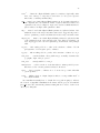
Appendix 1—Summary of program proj commands
35
Appendix 2—Summary of program nad2nad commands
39
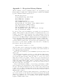
Appendix 3—Projection Library Entries
41
1
2
CONTENTS
3
Introduction
This is an interim document introducing changes and additions to release 4 of the
cartographic projection program proj originally described in Cartographic Projection Procedures for the Unix Environment—A User’s Manual (U.S. Geological
Survey Open-File Report 90–284). Because this report adds to, and does not replace, 90-284, new users of this system should obtain copies of the original report
for full documentation of the program. Users of release 3 proj should pay careful
attention to details of this new release which may affect current scripts and usage.
The principle reason for release 4 of proj is to increase the system’s portability
and usability. Two prime factors are considered in attempting to achieve this goal:
1. to make the C language source code compatible and compliant with ansi
language standards and posix procedural standards and
2. improve the modularity and encapsulization of the internals.
Although the earlier version, coded in K&R style C, was generally successful in
installation, occasional problems occurred that were due to site system peculiarities.
Hopefully, most of these have been eliminated.
Although the program proj is a reasonably flexible filter tool, it is limited in its
application to tasks that lend themselves to this mode of data processing. To help
software developers that need cartographic procedures embedded in their programs,
the cartographic procedures used in proj have been more carefully encapsulated
and thus make their inclusion in other application software a relatively easy task.
Individual projection procedures can now also have multiple states of initialization
so that processes such as datum transformations can be carried out within the same
program.
Acknowledgements
The author expresses his gratitude to the large number of individuals who have
contributed to the improvements and refinements of this software through questions,
suggestions and an occasional complaint. In particular, Jerry L. Bohannon has
made several suggestions that have been incorporated in the current release and
has supplied valuable source material. User feedback is a prime requirement in any
attempt to develop quality software.
In addition, special thanks to John P. Snyder for resolving technical problems
and supplying additional source material.
Release 3–4 Compatibility
Despite losing some upward compatibility, a few executional changes of release 4
of proj were necessary in order for options to maintain a reasonable relationship
with the revised internals of the system. Two proj control parameters found in
earlier releases are deleted: the -c for naming a source of ancillary control data and
+inv for specifying the inverse mode. The action of the -c option is replaced by
the more versatile initialization files and the +init parameter. Specifying inverse
projections is now done with the -I parameter. Inverse projections with invproj
name remains in effect.
Of lesser importance, the use of list as an argument to the +ellps and +proj
to obtain a listing of the available ellipsoid constants and projections has been
dropped from release 4. Run-line options -le and -lp now perform these respective
functions.
4
INTRODUCTION
New hyphen options.
To obtain a list of proj projections, the -l or -lp option will display a list of all
projections supported in the current installation (replaces the former +proj=list
option). An list with expanded explanation of each projection and associated parameters is obtained by using -lP. Examples of these option:
proj -l
qua_aut : Quartic Authalic
aea : Albers Equal Area
aeqd : Azimuthal Equidistant
airy : Airy
aitoff : Aitoff
alsk : Mod. Stererographics of Alaska
...
and
proj -lP
qua_aut : Quartic Authalic
PCyl., Sph.
aea : Albers Equal Area
Conic Sph&Ell
lat_1= lat_2=
aeqd : Azimuthal Equidistant
Azi, Sph&Ell
lat_0= guam
...
In general, the first supplementary line describes projection class (pseudocylindrical,
conic, . . . ), spherical or elliptical, . . . , and additional lines list options unique to
each projection.
For a short reminder of options associated with a single projection, the option
-l=id can be used where id is the accronym of the projection in question. For
example:
proj -l=lcc
lcc : Lambert Conformal Conic
Conic, Sph&Ell
lat_1= and lat_2= or lat_0=
Because proj may be using the initialization and default files (see Runtime
Initialization Files) the user may not be aware of the actual parameters being
used by proj. In addition, parameter misspelling or faulty usage can go unnoticed
because proj does not flag nor notify the user of parameters it does not know about.
The -v option is used to help verify selection and usage of projection parameters
(+ parameters) by displaying what values were actually used by the program. In
addition, parameters that were entered but not used are also noted and listed. For
example, the user performs the following proj execution:
# proj +proj=poly +lat_0=40 +lon0=-66 -v
with the following results printed by the -v printed at the beginning of the output:
# +proj=poly +lat_0=40 +ellps=clrk66
# following specified but NOT used
# +lon0=-66
New hyphen options.
5
The +lon0 parameter was not used and the user probably intended to use +lon_0.
Although the user might have sensed an error by examining the output and seeing
questionable values, other errors can be more subtle and difficult to detect. Also
note, the user is informed of the ellipsoid that was selected by the proj_def.dat
file.
The -E option is added as a convenience by causing the input coordinates to
be copied to the output stream prior the printing the projected results. Thus the
both forward and inverse values are placed side by side on the output shown in this
example output:
# sample points
65W 43d15N
-405817.61
-55 37.33
442931.70
4802414.53
4144652.95
created by the following script:
proj +proj=poly +lon_0=-60 -E <<EOF
# sample points
65W 43d15N
-55 37.33
EOF
When developing a new map or region for a plane coordinate system it is desirable to adjust the projection parameters to minimize the projection distortion
over the area. Although analytic methods may be used to determine these factors
it is often as easy to “cut and try” if a means to quickly check these values is available. Scale and information on other factors is important when using information
in cartesian space. To provide information about the performance of a projection
at a point the -V option provides an anotated lists of scale factors and other factors
at each location entered. Executing the following lines to determine characteristics
The following execution of proj shows the use of this switch for a point in the
Massachussetts Mainland spcs zone:
proj +init=nad27:2001 +units=us-ft -V
-70d36’30.872 41d38’54.192 A residence
which will produce the following output from proj:
Lambert Conformal Conic
Conic, Sph&Ell
lat_1= and lat_2= or lat_0
+init=/usr/local/lib/proj/nad27:2001 +units=us-ft +proj=lcc +a=6378206.4
+es=.006768657997291094 +lon_0=-71d30 +lat_1=42d41 +lat_2=41d43 +lat_0=41
+x_0=182880.3657607315 +y_0=0 +no_defs
Final Earth figure: ellipsoid
Major axis (a): 6378206.400
1/flattening: 294.978698
squared eccentricity: 0.006768657997
A residence
Longitude: 70d36’30.872"W [ -70.608575556 ]
Latitude: 41d38’54.192"N [ 41.648386667 ]
Easting (x):
843640.74
Northing (y): 237542.45
Meridian scale (h) : 1.00001069 ( 0.001069 % error )
Parallel scale (k) : 1.00001069 ( 0.001069 % error )
Areal scale (s):
1.00002138 ( 0.002138 % error )
Angular distortion (w): 0.000
Meridian/Parallel angle: 90.00000
Convergence : -0d35’55.663" [ -0.59879536 ]
Max-min (Tissot axis a-b) scale error: 1.00001 1.00001
6
INTRODUCTION
The “Final Earth figure” is shown to inform the user as to the effect of either
selecting one of the +R options or the fact that the projection is only for a spherical
figure. Discrepancies of the h and k values, which should be exactly 1., are due to
the limitations of determining derivatives by numeric rather than analytic methods.
To maintain a comple complete information log, the -v option is implicit with -V.
Additional points result in similar output and the user can also override the
forward-inverse mode of proj by making the the first character of a data line either
an upper of lower case f for forward or i for inverse. Any information after the
coordinates, such as the notation “A residence ” in the previous, example, are
printed out before the analytic information.
The meridian, h, and parallel, k, scale factors are the respective scales along
the meridian and parallel through the point and the areal scale factor, s, is the
area scale at the point. For conformal projections, h = k for all points and for
equal-area projections s will be constant for all points.
If two lines pass though the point the angle between these lines in geographic
space may be as much as twice the angular distortion, 2ω, different in cartesian space. Angular distortion is a common metric to quantify distortion of nonconformal maps by contouring either ω or 2ω. Angular distortion is always 0 for
conformal projections. Meridian-parallel angle, θ0 , is the angle between the meridian and parallel in cartesian space and is always 90◦ for conformal projections.
The convergence angle, γ, is the angle measured from the positive y cartesian
axis of the projection to true North—the meridian through the point. Most large
scale maps, such as the usgs quadrangle series, will have a margin figure with
utm grid and magnetic declination measured at the center of the sheet. “Grid
declination” is the convergence angle.
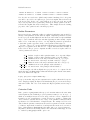
Scale factors a and b are the maximum and minimum scale error and define
the major and minor axis of the Tissot Indicatrix. The Tissot Indicatix, used as a
visual indication of map distortion, is based upon the concept of drawing a small
circle in geographic space and then portray a magnified image of this circle after
it has been projected. For conformal maps, the Indicatrix will remain a circle but
have a different size depending upon its location on the map. Equal-area maps will
have circular Indicatrixs at a point or along a line, but they will be elliptical in
shape elsewhere with only the area withing the ellipse remaining constant.
The -S option provides a summary of the above information as a field of values,
enclosed by <>, appended to the output record. Values incude meridinal and parallel
scale scale factors (h and k), area scale factor (s), angular distortion (ω) in decimal
degrees, and the major and minor axis of the Tissot Indicatrix (a, b).
Two projections of the conterminous U.S., Alber’s and Lambert Conformal
Conic, demonstrate characteristics of the -S option output as related to respective
equal area and conformal projections. Starting with the script for Albers Equal
Area:
proj -S +proj=aea +lon_0=90W -v <<EOF
-73 37
-110 44
EOF
proj -S +proj=lcc +lon_0=90W -v <<EOF
-73 37
-110 44
EOF
the following output was obtained:
# +proj=aea
1490786.23
-1586582.09
# +proj=lcc
+lon_0=90W +ellps=clrk66 +lat_1=29.5 +lat_2=45.5
4043351.48 <1.00965 0.990439 1 0.550448 0.990439 1.00965>
4860774.53 <1.00364 0.996375 1 0.208089 0.996375 1.00364>
+lon_0=90W +ellps=clrk66 +lat_1=33 +lat_2=45
Radius Parameters
1497189.34 4543009.70
-1588520.83 5351853.03
7
<0.995191 0.995191 0.990405 0 0.995191 0.995191>
<0.998284 0.998284 0.996571 0 0.998284 0.998284>
Note how the area scale factor (third term) remained unchanged for both points
as would be expected for an equal area projection but angular distortion and both
scale factors vary. In the case of the Lambert projection, the scale factors will
vary between points but for a particular point they are always equal in both directions and the angular distortion is always zero. This example shows the defining
properties of the equal area and conformal projections.
Radius Parameters
In previous releases of proj the radius of a spherical earth figure was specified by
the major axis parameter +a and either an explicit or implicit specification of +es=0
for those projections with elliptical form. In release 4 the radius of a spherical Earth
may be entered with the +R=radius and thus bypassing an unnecessarily complex
method. Use of +R= takes precedence over any elliptical parameter specifications
so that their possible appearance in the control parameter list is ignored.
Because of the need to specify an Earth radius that has a relationship with an
ellipsoid, a set parameters are introduced to compute this radius when an ellipsoid
is also selected. The projection computations will be treated as a sphere when one
of these parameters is selected:
+R A
+R V
+R a
+R g
+R h
+R lat a=φ
+R lat g=φ
Radius of a sphere with equivalent surface area of specified ellipse.
Radius of a sphere with equivalent volume of specified ellipse.
Arithmetic mean of the major and minor axis, Ra = (a + b)/2.
Geometric mean of the major and minor axis, Rg = (ab)1/2 .
Harmonic mean of the major and minor axis, Rh = 2ab/(a + b).
Arithmetic mean of the principle radii at latitude φ.
Geometric mean of the principle radii at latitude φ.
As an example, the Albers Equal Area projection is to be computed in the
spherical form for an Earth with a radius such that the sphere has the same surface
area as the Clarke 1866 ellipsoid:
# proj +proj=aea +ellps=clrk66 +R_A ...
For projections that only perform computations for a sphere, this method is preferable to simply specifying an ellipsoid and thus having the projection use the major
axis as the radius. The order of the radius and ellipsoid parameters is not important.
Cartesian Units
Basic operation of proj assumes that projected cartesian units are the same units
as the lengths associated with the projection parameter units (i.e. +a, +b, +x_0, . . .)
which are normally in meters. For some usage, such as for spcs computations, it
is useful to provide forward-inverse conversion between geographic coordinates and
other, non-meter, systems such as feet. Usage of the parameter +units=id allows
specification of several alternative of length measure. For example, if U.S. feet are
desired then the parameter +units=us-ft is used as a parameter and the cartesian
coordinates output in the forward mode and input in the inverse mode are in feet.
Usage of this parameter does not affect the units of the + projection parameters—
they must be in meters when using +units. The current list of units supported can
be obtained by using proj’s run-line option -lu:
8
km
m
dm
cm
mm
kmi
in
ft
yd
mi
fath
ch
link
us-in
us-ft
us-yd
us-ch
us-mi
INTRODUCTION
1000.
1.
1/10
1/100
1/1000
1852.0
0.0254
0.3048
0.9144
1609.344
1.8288
20.1168
0.201168
1./39.37
0.304800609601219
0.914401828803658
20.11684023368047
1609.347218694437
Kilometer
Meter
Decimeter
Centimeter
Millimeter
International Nautical Mile
International Inch
International Foot
International Yard
International Statute Mile
International Fathom
International Chain
International Link
U.S. Surveyor’s Inch
U.S. Surveyor’s Foot
U.S. Surveyor’s Yard
U.S. Surveyor’s Chain
U.S. Surveyor’s Statute Mile
The numeric value listed for reference purposes and is the value used to convert the
users cartesian coordinates to and from meters used for internal computations:
(x, y)meters
↔ conv × (x, y)usersunits
There is considerable variety of units of length measure and to include all units
used in just the last 200 years would only create confusion for the user. Other
situations such as the fact that the brass bar that established the standard for
the British yard shrank in length between 1853 and 1958 by about 5.5µ (Bomford,
1971) add to this confusion. Although such a small error seems trivial, it does
cause problems with high precision calculations associated with plane coordinate
systems. These factors along with the difficulty in resolving differences in conversion
factors for less common units the +units list is restricted to recent and well defined
conversions.
In order to allow other conversions to be imbedded within the cartographic
control parameters and thus be part of initialization and default control files the
+to_meter=frac may be used. The value of frac is a numeric value with properties
identical to those of the conversion number listed with the -lu proj option. As
shown in the -lu listing, the value may be expressed as a rational fraction with the
numerator and denominator separated with a /.
Initialization Parameter
Common usage of certain projections or projection features may be facilitated by
the projection parameters being predefined in initialization files. They are accessed
by the parameter +init=file:key where file is the name of the file containing the
control information and key identifies the particular set of parameters in the file
to be included as projection parameters. Conversion of spcs data (see ref) is case
for U.S. users where details of plane coordinate conversion are located in initialization files. For example, to convert 1927 North American Datum Massachussetts
Mainland coordinates to geographic coordinates:
$ proj -I +init=nad27:2001 <in_data >out_data
The file nad27 contains projection parameters for nad27 conversions and the key
2001 refers to the particular entry needed. Program proj will complain if either
the file cannot be found or there is no keyword or keyword data in the file.
Runtime Initialization and Default Files
9
Initialization files may be established by site personel responsible for proj administration or created by the individual user. Administrator files are located in
a directory specified by the user’s environment parameter PROJ_LIB and it is the
responsibility of the administrator to distribute documentation and instructions
of file contents and correct usage. Unless the administrator gives permission to
the user to install his files in the system area, the user will have to refer to his
initialization file with an absolute path:
$ proj +init=/home/me/lib/my_defs:proj5 ...
For Unix users, the ~ prefix to the file name will prepend the contents of the
HOME environment parameter. The user should refer to the next section on creating
initialization files.
Runtime Initialization and Default Files
Program proj is designed with runtime facilities to configure application definitions
and default parameters to the needs of the local environment. This is achieved
though the usage of two types of ascii text control files, initialization and default,
that are coded in a very simple control syntax that is identical for both types of
files—only the keyword usage differs.
Structure of the control files consists of identifiers in the form <keyword> followed
by a sequence of projection parameters. When processing the control file proj
scans for the specified keyword and when found, adds the parameters following the
keyword to the internal control list. Processing of parameters continues, ignoring
the occurrence of other keywords, until the <> character pair is encountered. When
<> is found after the desired keyword, processing of the control file is stopped, thus a
second occurrence of the keyword in the file is ignored. As with run-line projection
parameters, keywords and parameters are words that are groups of characters that
are separated by blanks, tabs or newlines. When a word begins with a # character
all input is ignored until the next newline character; thus comments may be added
to describe the data.
The following is a simple example of a initialization control file:
# a sample (comment line)
<myid1> proj=tmerc Ra <> # spherical
# transverse mercator
<pj-sph> Ra
# spherical form of
# the following
<pj-ell> proj=poly lon_0=90 ellps=airy <>
When the keyword myid1 is used the projection is set and the sphere of area equivalent to ellipse is selected but the ellipse and other parameters needed and must be
input by other means. The next two identifiers give sufficient detail to allow proj
to perform the projection. The pj-sph is an example where the second keyword is
ignored and its parameters are included as part of the first keyword specifications.
The first of the two types of control files are used by proj is the initialization file
explicitly referenced by the user with the +init control parameter. Its purpose is to
provide a convenient method to define commonly used and complex sets of control
parameters for map or grid coordinate system. For example, the standard zones
for the spcs systems are contained in two distributed initialization files nad27 and
nad83. Typically, the projection selection parameter, proj, is contained in these
files and there are sufficient parameters to fully qualify all options associated with
the projection.
Unless the +no_defs projections parameter has been given, the second control file (defaults file) is processed after all other projection parameters have been
input and after the projection name has been established. It is scanned for two
10
INTRODUCTION
keywords: general and a keyword that is the name of the selected projection. Parameters associated with general are default values associated with all projections
and typically defines a default ellipsoid. Projection parameters are those normally
associated with that projection in a particular geographic area of usage. A typical
example (from the proj distribution) would be:
<general> # for all projections
ellps=clrk66 # ellipsoid compatible
# with older U.S. maps
<>
<aea> # Conterminous U.S. map
lat_1=29.5
lat_2=45.5
<>
<lcc> # Conterminous U.S. map
lat_1=33
lat_2=45
<>
...
The name of this file is proj_def.dat and is located in the directory established
by the installer or pointed to bye the environment parameter PROJ_LIB (see next
section). For non-U.S. installations, it should be edited by the installer to reflect
local cartographic customs and usage. Program proj continues processing if the
file cannot be found or opened and in certain cases projection initialization will fail.
Paths of control files
The location of the initialization control file is controlled by how the user names
the +init file, how program proj was installed and the optional presence of the
environment parameter PROJ_LIB. If the file name begins with a / the file is assumed
to have an fully pathed name from the system root directory. If the name starts
with ./ or ../ is not defined, the file path is treated as relative to the current
working directory. When ~/ prefixes the file name, the users home directory, as
defined by the environment parameter HOME, is used as the root of the file name.
When simple initialization file names are used (those names without aforementioned prefixes) and in the case of the automatic default file, the location of the files
is controlled by proj installation or the user’s environment parameter PROJ_LIB. In
case of the environment parameter, the user is overriding the installation defaults
and establishing his or her own initialization and default definition file path. To
set the environment path do either
setenv PROJ_LIB /usr/local/lib/proj
when using csh(1) or
PROJ_LIB=/usr/local/lib/proj
export PROJ_LIB
when using sh(1) or ksh(1). If the user always wants these settings, then they can
be included in the .login or .profile files.
Caveats
The initialization and default files provide a useful tool to configure proj to a wide
variety of conditions that best fit local needs and thus ease the usage of proj in
the performance of routine tasks by less knowledgeable and infrequent users. But
care should be exercised in their usage. Certain options may be included in the
Runtime Initialization and Default Files
11
automatic file that may cause hidden and unintended operations. For example,
inclusion of parameters such as R_A or R_V in the automatic files may cause unintended spherical computations when it was thought that an elliptical projection
was explicitly specified.
12
INTRODUCTION
13
Datum Conversions
The use of satellites and other technologic improvements in first order surveying
have allowed geodesists to refine the knowledge of the shape of the Earth. Along
with these refinements came the inevitable process of standardizing the definition
of the approximating ellipsoid and establishing an international reference datum.
Prior to this, the ellipsoids and datums were established by long line precision
surveying and astronomical observation. The processing of the measurements of
these surveys let to establishment of ellipsoids which were best fits to local conditions and not the entire Earth and datums which were arbitrary to the surveyor’s
network. But because this surveying relied upon the use of the spirit level for alignment of instruments with the horizontal plane (the geoid) they were susceptible to
perturbations of the gravity field and thus only useful for local purposes.
Until recently, the reference system for North America has been the North
American Datum of 1927 (nad27) which used Clarke’s 1866 ellipsoid and had its
origin at Meade’s Ranch in Kansas. But because of technical geodetic surveying
problems with nad27 and an interest in standardizing the reference system on an
international basis, the North American Datum of 1983 reference system nad83 has
been chosen to replace nad27. This system is based upon the Geodetic Reference
System of 1980 (grs80) which is geocentric (origin is the center of the Earth’s
mass) and uses an ellipsoid approximating the entire Earth.
There are several methods for conversion of geographic data between datums
but the most convenient and perhaps common are the Molodensky formula and
the nadcon (Dewhurst, 1990) used for North American Datum conversions. The
Molodensky method is often used for international conversions but is considered to
only have a conversion accuracy of 5–10m in United States regions. The nadcon
method uses of a grid of longitude–latitude corrections from which a correction value
can be interpolated for any non-nodal point. The correction grid is determined by
minimum curvature gridding of corrections for control points whose location had
been accurately determined by both nad27 and nad83 surveying methods. Error
in conversion with nadcon is generally considered to be less than a meter (0.15m
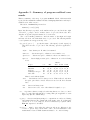
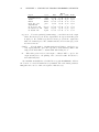
for most of the conus region) but may suffer in regions of poor control. Table 1 is
a summary of the nadcon grid regions.
Table 1: nadcon correction regions.
Region
Conterminous U.S.
Alaska
Hawaii
Puerto Rico and
Virgin Islands
St. George Is., AK
St. Lawrence Is., AK
St. Paul Is., AK
nad2nad
-r region
Extent
West South
East
131 W
166◦ E
161◦ W
63 W
128◦ W
154◦ W
20 N
46◦ N
18◦ N
50◦ N
77◦ N
23◦ N
prvi
68◦ W
64◦ W
17◦ N
19◦ N
◦
56 N
62◦ N
57◦ N
57◦ N
64◦ N
58◦ N
24◦
37◦
34◦
41◦
42◦
32◦
41◦
38◦
50◦
48◦
◦
171 W
172◦ W
171◦ W
◦
◦
169 W
68◦ W
169◦ W
◦
North
conus
alaska
hawaii
stgeorge
srlrnc
stpaul
◦
High Precision GPS Network
Florida
Maryland
Tennessee
Washington–Oregon
Wisconsin
FL
MD
TN
WO
WI
88◦
80◦
91◦
125◦
94◦
W
W
W
W
W
80◦
74◦
81◦
116◦
88◦
W
W
W
W
W
N
N
N
N
N
N
N
N
N
N
Recent releases (circa July, 1993) of nadcon tables also include tables for con-
14
DATUM CONVERSIONS
version between the High Precision gps Networks (hpgn) and nad83. Little information about the hpgn was distributed with the tables so usage is available but
not defined at the moment. These tables are for state regions.
Program nad2nad.
For conversion of data between nad27 and nad83 datums the software distribution
now includes the program nad2nad. It performs in a manner similar to program
proj and has several of the same runline options so users familiar with proj should
have little trouble with learning nad2nad. Besides performing datum conversions
it will perform spcs and utm conversions for both input and output thus allowing
both geographic as well as grid data to be processed.
The internal functioning of nad2nad is a three step process:
1. process input data and, if selected, convert data from grid system coordinates
to geographic coordinates,
2. if nadcon region selected, convert geographic data between datums, and
3. process output data and, if selected, convert to grid system coordinates.
Control of the input and output steps are by means of the respective -i and -o
runline options which have an identical list of arguments:
27 — data is in nad27 datum. This is the default state.
83 — data is in nad83 datum.
utm=zone — data in utm coordinates for identified zone (numeric value between
1 and 60).
spcs=zone — data in spcs coordinates for identified State zone (see Table 2).
bin — data in binary form.
rev — reverse normal longitude-latitude or x-y order of data.
feet — data is in U.S. Surveyor’s feet, otherwise in meters. Must be used in
conjunction with spcs option.
hpgn=zone — data is in hpgn datum for zone listed in Table 1.
These options represent the state of the data at respective input and output of
steps 1 and 3 and thus determine the necessary actions to be taken to convert the
information to intermediate geographic coordinates required for datum shift. More
than one option can be used and in this case they may be in a comma separated
list or separate -i or -b options as shown by the following:
# nad2nad -i 83 -i spcs=1001 -i feet ...
# nad2nad -i 83,spcs=1001,feet ...
Option order is not important.
Step 2 of nad2nad is controlled by the -r <region> option which determines
which nad27–nad83 zone listed in Table 1 is to be used. When this option is
specified the the -i and -o must indicate different datums, thus
# nad2nad -i 27 -o 83 -r conus ...
is correct usage, while
# nad2nad -i 27 -o 27 -r conus ...
# nad2nad -r conus ...
Program nad2nad.
15
are incorrect usage. The following is an example where geographic nad27 coordinates are to be converted to geographic nad83 coordinates:
# nad2nad -i 27 -o 83 -r conus <<EOF
-71d15 44d20’15
120W 30N
87d30 52d14
EOF
which produces the output:
71d14’58.27"W
120d0’3.181"W
*
*
44d20’15.227"N
30d0’0.348"N
Note that the last coordinate is outside the conus region.
Because changing datums of grid system data is common, the nad2nad utm and
spcs options may be used to process these systems. In this case, Massachussetts
Mainland zone nad27 coordinates in feet are converted to nad83 values in meters
by:
# nad2nad -i 27,spcs=2001,feet -o 83,spcs=2001 -r conus <<EOF
840000 230000
EOF
with the results being:
273193.78
820117.57
Similarly, the same data can be converted to utm, zone 19 coordinates by:
# nad2nad -i 27,spcs=2001,feet -o 83,utm=19 -r conus <<EOF
840000 230000
EOF
resulting in output of:
364916.74
4609733.79
The -r option may be omitted so that there is no datum transformation. This
allows nad2nad to be used for purposes such as converting spcs grid coordinates
to and from utm grid coordinates, conversion of grid coordinates from one zone
to an adjacent zone, or simply converting geographic coordinates to and from dms
and decimal degrees formats. The previous example could be a simple conversion
from spcs to utm in the nad27 datum as performed by:
# nad2nad -i 27,spcs=2001,feet -o 27,utm=19 <<EOF
840000 230000
EOF
with the results:
364869.08
4609509.76
To do this operation with proj would create considerably more system overhead
due to two copies of the program executing and data piping operations.
16
DATUM CONVERSIONS
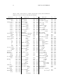
Table 2: List of State Plane Coordinate System Zones (spcs) and identification
numbers for 1927 and 1983 North American Datums.
State Zone
Alabama East
West
Alaska Zone 1
Zone 2
Zone 3
Zone 4
Zone 5
Zone 6
Zone 7
Zone 8
Zone 9
Zone 10
Arizona East
Central
West
Arkansas North
South
California I
II
III
IV
V
VI
VII
Colorado North
Central
South
Connecticut
Delaware
Florida East
West
North
Georgia East
West
Hawaii 1
2
3
4
5
Idaho East
Central
West
Illinois East
West
Indiana East
West
0
27
101
102
5001
5002
5003
5004
5005
5006
5007
5008
5009
5010
201
202
203
301
302
401
402
403
404
405
406
407
501
502
503
600
700
901
902
903
1001
1002
5101
5102
5103
5104
5105
1101
1102
1103
1201
1202
1301
1302
0
83
State Zone
101
102
5001
5002
5003
5004
5005
5006
5007
5008
5009
5010
201
202
203
301
302
401
402
403
404
405
406
Iowa North
South
Kansas North
South
Kentucky North
South
Louisiana North
South
Offshore
Maine East
West
Maryland
Massachusetts Mainland
Islands
Michigan East
Central/m
West
North
Central/l
South
Minnesota North
Central
South
Mississippi East
West
Missouri East
Central
West
Montana
North
Central
South
Nebraska
North
South
Nevada East
Central
West
New Hampshire
New Jersey
New Mexico East
Central
West
New York East
Central
West
long island
501
502
503
600
700
901
902
903
1001
1002
5101
5102
5103
5104
5105
1101
1102
1103
1201
1202
1301
1302
0
27
1401
1402
1501
1502
1601
1602
1701
1702
1703
1801
1802
1900
2001
2002
2101
2102
2103
2111
2112
2113
2201
2202
2203
2301
2302
2401
2402
2403
0
83
1401
1402
1501
1502
1601
1602
1701
1702
1703
1801
1802
1900
2001
2002
2111
2112
2113
2201
2202
2203
2301
2302
2401
2402
2403
2500
2501
2502
2503
2600
2601
2602
2701
2702
2703
2800
2900
3001
3002
3003
3101
3102
3103
3104
2701
2702
2703
2800
2900
3001
3002
3003
3101
3102
3103
3104
State Zone
North Carolina
North Dakota North
South
Ohio North
South
Oklahoma North
South
Oregon North
South
Pennsylvania North
South
Rhode Island
South Carolina
North
South
South Dakota North
South
Tennessee
Texas North
North Central
Central
South Central
South
Utah North
Central
South
Vermont
Virginia North
South
Washington North
South
West Virginia North
South
Wisconsin North
Central
South
Wyoming East
East Central
West Central
West
American Samoa
Guam Island
Puerto Rico, Virgin Is.
1
(St. Croix) 2
0
27
3200
3301
3302
3401
3402
3501
3502
3601
3602
3701
3702
3800
3901
3902
4001
4002
4100
4201
4202
4203
4204
4205
4301
4302
4303
4400
4501
4502
4601
4602
4701
4702
4801
4802
4803
4901
4902
4903
4904
5300
5400
0
83
3200
3301
3302
3401
3402
3501
3502
3601
3602
3701
3702
3800
3900
4001
4002
4100
4201
4202
4203
4204
4205
4301
4302
4303
4400
4501
4502
4601
4602
4701
4702
4801
4802
4803
4901
4902
4903
4904
5200
5201
5202
17
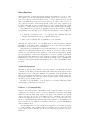
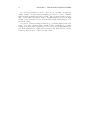
New and Revised Projections
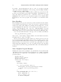
The seven new projections that have been added to release 4 of program proj are
listed in Table 3. Graphic examples are shown in Figures 1–4. In addition, new
options have been added to the some of the existing projections as shown in Table 4.
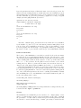
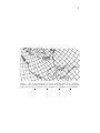
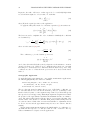
Figure 1: New Zealand Map Grid projection, with shorelines and 1◦ graticule.
18
NEW AND REVISED PROJECTIONS
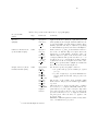
Table 3: Projections new to release 4 of program proj
Projection Name
(Alias)
Type∗
Parameters
Comments
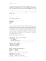
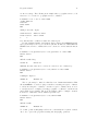
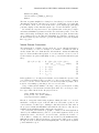
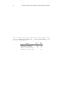
Two Point Equidistant
(Doubly Equidistant)
SI
+proj=tpeqd
+lon 1=λ1
+lat 1=φ1
+lon 2=λ2
+lat 2=φ2
The central points, P (λ1 ,φ1 ) and P (λ2 ,φ2 ), are on a great
circle coincident with the cartesian x-axis and the cartesian origin is midway between the central points and y is
positive to the left of the line from P1 to P2 . Distance
from any point to the two central points is true great
circle (geodesic) distance. Scale is correct along the line
through P1 –P2 . See Figure 3.
New Zealand Map Grid
CEI
+proj=nzmg
The central meridian (+lon 0) and parallel (+lat 0) are
fixed at 173◦ E and 41◦ S respectively and the International (+ellps=intl) elliptical figure is fixed. False easting and northings are also fixed at (x 0=)2,510,000m and
(y 0=)6,023,150m. See Figure 1.
landsat
CESI
+proj=lsat
+lsat=n
+path=p
This projection (not shown) is for use with landsat
satellite data and is a limited form of the more general
Space Oblique Mercator projection. The landsat satellite number, n, must be in the range 1–5 and the path
number, p, must be in the ranges 1–251 for n = 1, 2, 3 or
1–233 for n = 3, 4.
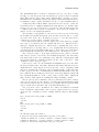
50 United States Modified
Stereographic
CESI
+proj=gs50
The central meridian (+lon 0) and parallel (+lat 0) are
fixed at 120◦ W and 45◦ N respectively. Selection of ellipsoid or spherical conversion is performed by conventional
means, but actual values used are fixed at respective
Clarke 1866 and its equivalent sphere radius, 6,370,997m.
See Figure 4B.
Alaska Modified
Stereographic
CESI
+proj=alsk
The central meridian (+lon 0) and parallel (+lat 0)
are fixed at 152◦ W and 64◦ N respectively. Control of
elliptical-spherical figure is fixed an performed in an identical manner to the above 50 U.S. Modified Stereographic.
See Figure 4A.
Lee Oblated Stereographic
CSI
+proj=lee os
The central meridian (+lon 0) and parallel (+lat 0) are
fixed at 165◦ W and 10◦ S respectively. See Figure 4D.
Miller Oblated
Stereographic
CSI
+proj=mill os
The central meridian (+lon 0) and parallel (+lat 0) are
fixed at 20◦ E and 18◦ N respectively. See Figure 4C.
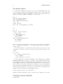
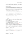
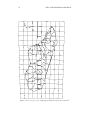
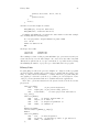
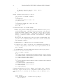
Laborde
CEI
+proj=labrd
+azi=Az
k 0=k0
This projection is only used for the Madagascar Grid
Map (see Figure 2) where the parameters should always be specified as: ellps=intl, lon_0=46d2613.95E’,
lat_0=18d54S, azi=18d54, k_0=.9995, x_0=400000 and
y_0=800000
∗
C–Conformal, A–Equal-Area, S–spherical, E–elliptical, I–inverse
19
Table 4: Projections revised in release 4 of program proj
Projection Name
(Alias)
Type∗
Parameters
Comments
Mercator
(Wright)
CEI
+proj=merc
+lon ts=φts
or
+k 0=k0
Applications should be limited to equitorial regions, but
it is frequently used for navigational charts with true scale
(φs ) specified within or near the chart’s boundary. Alternatively, equitorial scale may be adjusted by specifying
k0 . When neither is specified, scale is true at the Equator.
Lambert Conformal Conic
(Conical Orthomorphic)
CEI
+proj=lcc
+lat 0=φ0
secant
+lat 1=φ1
+lat 2=φ2
tangent
+lat 1=φ1
+k 0=k0
In the secant case, φ1 and φ2 are the latitudes of intersection of the cone with the ellipsoid or sphere and for the
tangent case, φ1 is the latitude of tangency of the cone
with the ellipsoid or sphere. Scale is true at the secant
or tangency latitudes. The special cases where φ1 = −φ2
(secant mode) or φ1 = 0 (tangent mode) that configure
a cylinder are not allowed. Use Mercator for these cases.
If lat 0 is not specified, then 0◦ (Equator) is assumed in
the secant case and φ1 in the tangent case.
Oblique Mercator (Rectified Skew Orthomorphic)
CEI
+proj=omerc
+k 0=k0
+lat 0=φ0
+no rot
+no uoff
+rot conv
two point
+lon 1=λ1
+lat 1=φ1
+lon 2=λ2
+lat 2=φ2
azimuthal
+alpha=αc
+lonc=λc
Two means of specify cartographic control are:
∗
C–Conformal, E–elliptical, I–inverse
1. two points on the projection centerline (λ1 , φ1 ) and
(λ2 , φ2 ),
2. a point of origin at (λc , φ0 ) and an azimuth, measured clockwise from North, of the projection centerline αc .
The presence of the +alpha option determines which
method is used. The projection centerline approximates
a geodesic.
Unless the +no_rot option is specified, the coordinates
are rotated by αc (computed internally with the two
point method) or by the origin convergence angle when
+rot_conv is specified. In some cases, an offset in the
pre-rotated axis may need to be suppressed with the
+no_uoff option. The scale factor, k0 , applies to the
projection origin.
Initialization will fail if parameters define a nearly transverse or normal Mercator projection.
20
NEW AND REVISED PROJECTIONS
Figure 2: Laborde projection of Madagascar with shorelines and 1◦ graticule.
21
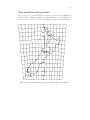
Figure 3: Two Point Equidistant projection, with shorelines and 5◦ graticule.
Central points at Seattle, Washington and Charlotte Amalie, U.S. Virgin Islands
(+proj=tpeqd +lon 1=122d20w +lat 1=47d36n +lon 2=64d54w +lat 2=18d21n).
22
NEW AND REVISED PROJECTIONS
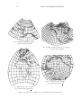
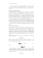
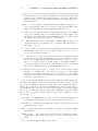
A – Alaska Modified Stereographic
5◦ graticule (+proj=alsk)
B – 50 United States Modified Stereographic
5◦ graticule (+proj=gs50)
D – Lee Oblated Stereographic
10◦ graticule (+proj=lee os)
C – Miller Oblated Stereographic
10◦ graticule (+proj=mill os)
Figure 4: Modified Stereographic projections with shorelines and graticules
23
Programming with the Cartographic Library
Use of cartographic projections in computer applications is varied and potentially
complex and, although a program such as proj can serve variety of needs, there are
many situations where more specialized programs are more appropriate or required.
To support alternate applications, the software was developed to be modular and
encapsulated so that the application programmer can concentrate efforts on the
unique needs of the application and not on the details of cartographic mathematics. This section describes usage of the principle entries of the projection library
and Appendix 3 contains a summary of all the entries to procedures of potential
programmatic interest.
Basic Usage
A cartographic projection is similar to the standard transcendental functions included in the compilers mathematics library such as sin(x) to compute sin x and
asin(x) to compute the inverse, sin−1 x. But unlike the transcendental functions,
the forward, P , and inverse, P −1 , cartographic projection functions have a multivariate argument and a bivariate return value:
(x, y) = P (λ, φ, · · ·)
(λ, φ) = P −1 (x, y, · · ·)
(1)
(2)
where x and y are the cartesian coordinates, usually in meters, and λ and φ are
the respective longitude and latitude geographic coordinates in radians. There is
always either the Earth’s radius, R, or the major ellipsoid major axis, a, and one
of the means of specifying ellipsoid shape that are part of the remaining P arguments. The actual number of function arguments is reflected in the tabulation of
the cartographic parameters previously described in the user’s sections and include
such elements as central meridian, standard parallels, false easting and northing,
... .
Because of the large number of selectable projections, each with their own special
list of arguments, the following method was chosen to simplify the number of library
entries needed by the programmer to the following prototypes defined in the header
file projects.h:
PJ *pj_init(int, char **);
UV pj_fwd(UV, PJ *);
UV pj_inv(UV, PJ *);
void pj_free(PJ *);
The complexity of this system is not in programmatic usage as described in the
following text, but in understanding and properly using the cartographic control
parameters.
The procedure pj_init must be called first to select and initialize a projection.
Parameters for the projection are passed in a manner identical with the normal
C program entry point main: a count of the number of parameters and a list of
pointers to the characters strings containing the parameters. In this case, the
parameter strings are those cartographic parameters discussed in the section on
using program proj and the projection tables. This also includes references to
initialization files and the use of the default file.
If the initialization call to pj_init fails, then a null or (PJ *)0 value is returned.
Otherwise, pj_init returns a pointer that is used as an argument with the forward,
pj_fwd, and inverse, pj_inv, projection functions. The first argument argument
to the forward and inverse projection function and the function return is a type
declared (in the header file projects.h) as:
24
PROGRAMMING WITH THE CARTOGRAPHIC LIBRARY
typedef struct { double u, v; } UV;
where u and v respective x and y cartesian coordinates or respective longitude, λ,
and latitude, φ, geographic coordinates 1 in radians. If either the forward or inverse
function fail to perform a conversion, both u and v in the returned structure are
set to HUGE_VAL as defined in the math.h header file.
Two additional notes should be made about the header file projects.h: it
contains includes to the system header files stdlib.h and math.h, and several predefined constants such as multipliers DEG_TO_RAD and RAD_TO_DEG to respectively
convert degrees to and from radians.
To illustrate usage, the following is an example of a filter procedure, example1.c,
designed to convert input pairs of decimal latitude and longitude values in decimal
degrees to corresponding cartesian coordinates using the Polyconic projection with
a central meridian of 90◦ W and the Clarke 1866 ellipsoid:
#include <stdio.h>
#include <projects.h>
main(int argc, char **argv) {
static char *parms[] = {
"proj=poly",
"ellps=clrk66",
"lon_0=90W",
"no_defs"
};
PJ *ref;
UV data;
if ( ! (ref = pj_init(sizeof(parms)/sizeof(char *), parms)) ) {
fprintf(stderr, "Projection initialization failed\n");
exit(1);
}
while (scanf("%lf %lf", &data.v, &data.u) == 2) {
data.u *= DEG_TO_RAD;
data.v *= DEG_TO_RAD;
data = pj_fwd(data, ref);
if (data.u != HUGE_VAL)
printf("%.3f\t%.3f\n", data.u, data.v);
else
printf("data conversion error\n");
}
exit(0);
}
Assuming that the header file has been installed in /usr/local/include and the
projection library in /usr/local/lib, then the example can be compiled and
loaded by:
# cc -I/usr/local/include example1.c -L/usr/local/lib -lproj -lm
To test the program, the script
# a.out <<EOF
0 -90
33 -95
1
An argument can be made that giving both coordinates systems the same type name is
bad style, but the author has found through experience that this method is generally much more
convenient because the functions are often used interchangeably.
Limiting Selection of Projections
25
77 -86
EOF
should give the results:
0.000
0.000
-467100.408
100412.759
3663659.262
8553464.807
The previous example can be expanded to create a more flexible program with
runtime selection of projection parameters by removing the parms declaration and
initialization, and substituting the pj_init parameters with the arguments from
main entry:
if ( ! (ref = pj_init(--argc, ++argv)) ) {
Recompiling the program and executing it as:
# a.out proj=poly ellps=clrk66 lon_0=-90 no_defs
will give the same results as the original program. The use of + parameter prefix as
in the case with program proj is only to flag the runline values as non-files, much
in the same manner that - is uses to flag options. In this case, runline files are not
part of the program, so use of + is not needed.
When executing pj_init the projection system allocates memory for the structure PJ. This allocation is complex and consists of two or more memory allocations to assign substructures referenced within PJ. Although the previous examples
did not require its usage, certain applications are foreseen where repeated calls to
pj_init are made to re-initialize a projection with different parameters. The function pj_free should be used to ensure proper memory deallocation of a previously
initialized PJ pointer when the process has no further need for the structure.
Limiting Selection of Projections
Many applications will only need a small subset of the projections contained in the
library libproj.a, but unless some action is taken, all of the projections will be
linked into the final process. This is not a problem unless the memory requirements
of the application are to be kept small or access to projections is to be restricted.
If there is a need to limit the number of projections, a simple two-step process
needs to followed. First creat a header file, my_list.h for example, that contains
a list of macro calls PROJ_HEAD(id,text), one for each projection to be part of the
application program. Argument id is the acronym of the projection and argument
text is the ascii string describing the program (what appears after the colon in
proj’s -l execution. The header file, nad_list, for program nad2nad is a an
example:
/* projection list for program nad2nad */
PROJ_HEAD(lcc, "Lambert Conformal Conic")
PROJ_HEAD(omerc, "Oblique Mercator")
PROJ_HEAD(poly, "Polyconic (American)")
PROJ_HEAD(tmerc, "Transverse Mercator")
PROJ_HEAD(utm, "Universal Transverse Mercator (UTM)")
An easy way to create this list is to copy and edit the file pj_list.h in the source
distribution, which contains the entire listing of available projections, and edit out
of the copy all lines of unwanted projections.
Next, in one of the program code modules that includes the header file
projects.h, preceed the include statement with:
#define PJ_LIST_H "my_list.h"
26
PROGRAMMING WITH THE CARTOGRAPHIC LIBRARY
Be careful to only put this include in only one of the code modules because this
define action causes the initialization of the global pj_list and multiple initializations will cause havoc with the linker.
When no action is taken to limit the number of linked projections, the module
pj_list.o from the library is used which causes linkage of all distributed projections. The savings in program size can be considerable. In the case of program
nad2nad, the use of the above process yields a program of about 48kbytes while
ignoring the process creates a program of about 154kbytes—more than three times
larger.
Error Handling
Error handling in the projection system is performed in much the same manner
as the standard ansi C library procedures. In cases where a functional value is
returned, the returned value assumes a special state such as a null pointer or double
precision HUGE_VAL. The system also sets a global type int value pj_errno to a
non-zero value indicating the cause of the error. Although similar to the ansi
standard’s errno, it differs in two properties: it is never used as a macro and it, as
well as errno, is reset to zero at each execution of pj_init, pj_fwd and pj_inv.
To provide users with an indication of the type of error encountered, the function
char *pj_strerrno(int pj_errno)
may be used to obtain a string for display. Similar to the ansi C function strerror,
the string pointed to cannot be modified.
The projection system uses negative values for pj_errno for all errors detected
by projection system tests. If C library system errors occur during execution of the
projection system, thus causing errno to return a positive value, and the projection
system otherwise does not detect an error, the value of pj_errno will be set to errno
and the functional results will be set to the error values. In these cases, the string
pointer returned by the function pj_strerrno will be that of the C library function
strerror.
More Complete Program Example
With the same basic criteria of example1.c program with the added restriction that
only Transverse Mercator and Polyconic projections are to be computed, dms input
data and better error diagnostics of the initialization, the following example2.c
program is written:
#include <stdio.h>
#define PJ_LIST_H "examp2.h"
#include <projects.h>
main(int argc, char **argv) {
PJ *ref;
UV data;
char lat[40], lon[40];
if ( ! (ref = pj_init(argc, argv)) ) {
fprintf(stderr, "Projection initialization failed\n"
"because: %s\n", pj_strerrno(pj_errno));
exit(1);
}
while (scanf("%39s %39s", lat, lon) == 2) {
data.u = dmstor(lon, 0);
data.v = dmstor(lat, 0);
data = pj_fwd(data, ref);
if (data.u != HUGE_VAL)
Library Lists
27
printf("%.3f\t%.3f\n", data.u, data.v);
else
printf("*\t*\n");
}
exit(0);
}
and where header file examp2.h contains:
PROJ_HEAD(poly, "Polyconic (American)")
PROJ_HEAD(tmerc, "Transverse Mercator")
Compiling and linking the program in the same manner as the first example
and executing with the following script:
# a.out proj=tmerc ellips=clrk66 lon_0=90w <<EOF
33.3 -90.55
44d15’7.5 87d10’15.4w
EOF
should give the results:
-51226.063
225953.937
3685962.942
4905510.287
The resulting total size of this program with limited projections was 28,712 bytes
versus 117,988 bytes for the first example. Of course, these size values vary with
different host systems but it does give an indication of possible memory savings
when limiting the number of projection procedures linked into the program.
Library Lists
Program proj as well as the previous examples are designed as filter programs
executed from the run-line and not interactive programs with user dialog capability. To fully discuss mechanisms to construct interactive programs using the
cartographic procedures is beyond the scope of this report, but description of some
of the projection system internals can be useful in interactive applications.
There three option list structures in the system described in the header file
projects.h:
struct PJ_LIST {
char
*id;
/* projection keyword */
void
*(*proj)(); /* projection entry point */
char
*const*name;
/* basic projection full name */
} pj_list[];
struct PJ_ELLPS {
char
*id;
/* ellipse keyword name */
char
*major; /* a= value */
char
*ell;
/* elliptical parameter */
char
*name; /* comments */
};
#ifndef PJ_ELLPS__
extern struct PJ_ELLPS pj_ellps[];
#endif
struct PJ_UNITS {
char
*id;
/* units keyword */
char
*to_meter; /* multiply by value to get meters */
char
*name; /* comments */
};
28
PROGRAMMING WITH THE CARTOGRAPHIC LIBRARY
#ifndef PJ_UNITS__
extern struct PJ_UNITS pj_units[];
#endif
The first, PJ_LIST, simplified for clarity here, has already been described when
discussing the alteration of the list of projections to be linked into a program. But
it, as well the others, can be used in interactive option displays (program proj
performs a display of these lists through the -lp, -le and -lu run-line options).
In each list, the id pointer refers to the argument value for the proj=, ellps=
and units= initialization parameters and the associated name points to a more human readable string describing the entry. In an interactive program, the name entry
can be displayed in a scrolled list and, maintaining an equivalence of indicies, use
the index returned by user selection to generate the string needed by the argument
list for pj_init.
Matrix Datum Conversion.
The matrix method of datum conversion is the use of a two dimensional matrix of
correction values to be added to an input of one datum to determine the value in
another datum. The row-column interval of the matrix is constant and sufficiently
spaced to allow semi-linear interpolation of correction values not located on a node
by the bivariate four-point formula (Eqn. 25.2.66, p. 882, Abramowitz and Stegun,
1965):
f (ui + ph, vj + qk)
=
p
q
h
k
=
=
=
=
(1 − p)(1 − q)fi,j + p(1 − q)fi+1,j
+q(1 − p)fi,j+1 + pqfi+1,j+1 + O(h2 )
(u − ui )/h
(v − vj )/k
ui+1 − ui
vi+1 − vi
(3)
(4)
(5)
(6)
(7)
(8)
In the application of correcting nad27 datum to nad83 datum the respective u and
v are longitude and latitude and f is a value to be added to the nad27 coordinates
in order to convert to nad83. The inverse correction is determined by simple, direct
iteration of detemining a point that produces a corrected value.
Usage of this system is similar to the usage of the projection system: creating
and initializing a control structure and subsequent calls to the correction procedure.
Prototypes defined in the header file projects.h are:
struct CTABLE *nad_init(char *)
UV nad_cvt(UV, int, struct CTABLE *)
void nad_free(struct CTABLE *)
Execution of nad_init with a string argument defining the name of a correction
matrix file covering the region of interest will create and return a pointer to the
control structure for this region. Pathing for this file follows the same rules as
the projection default and initialization files with the added factor of the directory
nad2783. If the initialization fails, a null pointer is returned.
Procedure nad_cvt returns the geographic coordinates of the first argument as
defined by the CTABLE structure pointed to by the third argument. If the second
argument is non-zero, the inverse correction is made, otherwise the forward correction. When coordinates are outside the region defined by the CTABLE structure,
HUGE_VAL is returned. When doing inverse correction it is possible to move outside
the region near the boundary, thus returning HUGE_VAL, even though the argument
point is within the region.
Projection Approximations
29
The procedure nad_free closes the structure CTABLE and returns allocated memory to the system. When creating a CTABLE structure, the correction matrix is read
into memory and a considerable increase in program memory requirements may be
expected.
Projection Approximations
Cartographic projections can be computationally complex and some uses will increase this complexity by requiring multiple projection evaluations and other computations for each point processed. Thus, when a large number of points are to
be processed, a considerable amoung of computer processing will be used in the
transformation process. Although costs of computing have declined and computer
speed has substantially increased, the geometric increase in the volume of data as
well as the need for fast processing (often for interactive graphics) encourages the
use of effective alternatives to the use of the analytic projection procedures.
Snyder (1985) reviews projection approximations but limits discussion to power
series developed by either Taylor series expansions or least-squares methods. These
techniques often work, but it is desirable to follow more traditional function approximation methods that are based upon the premise of minimizing the maximum
error of the approximation: minimax. True minimax approximations are difficult
to determine, but there is a simple and easily applied method that nearly reaches
this goal.
Chebyshev Approximation
The approximation method used in this system is the Chebyshev method because
of its property of error determination, its near minimax characteristics and the ease
in determining its coefficients. Application of this method to univariate functions
is well known, but neither theory nor application references for multivariate applications have been located. However, practice has shown that the following intuitive
expansion of the Chebyshev method can work for bivariate cartographic applications and most of the procedures used in this system were developed by adaptation
of the univariate procedures described in Numerical Recipes in C (Press, et al.,
1988).
In the univariate case, a function, f (u), may be approximated over the argument
inverval −1 ≤ u ≤ 1 by:
N
X
0
(9)
f (u) ≈
ci Ti (u)
i=0
using Fox and Parker (1968) notation where the prime indicates that the c0 term
is halved at evaluation and where Ti (u) is the Chebyshev polynomial of degree n.
The c0 coefficients are determined by:
N
cn =
2 X
f (uk ) cos(nuk )
N +1
(10)
k=0
where
2k + 1 π
uk = cos
·
(11)
N +1 2
Because |Tn (u)| ≤ 1 for −1 ≤ u ≤ 1, and (9) is exact for N = ∞, the accuracy
of the approximation of a non-infinite N can be assessed by examination of the
coefficients cn . When the value of the coefficients converge to zero with increasing
n, a value of N can be selected for an approximation with the maximum error, |E|,
of this truncation being:
∞
X
|E| ≤
|cn |.
(12)
n=N +1
30
PROGRAMMING WITH THE CARTOGRAPHIC LIBRARY
In practice, the value of N is set to a value expected to be considerably higher than
needed and then adjusted to a lower value, N 0 , such that:
N
X
|E| ≤
|cn |.
(13)
n=N 0 +1
where |E| is the required precision of the application.
To apply the Chebyshev method to a bivariate expression, (9) is rewritten as:


N
M
X
X
0
0
f (u, v) ≈
(14)
ci,j Tj (v) Ti (u)
i=0
j=0
The braces are used to emphasize the order of evaluation. Similarly, the coefficients
are determined by:
"
#
N
M
2 X
2 X
f (uk , vl ) cos(mvl ) cos(n, uk )
(15)
cn,m =
N +1
M +1
k=1
l=0
where uk is the same as (11) and:
vl = cos
2l + 1 π
·
M +1 2
(16)
The coefficients, pi,j , for the bivariate power series
f (u, v) ≈
N X
M
X
pi,j ui v j
(17)
i=0 j=0
can be derived from the Chebyshev series by adaptation of the univatiate conversion
described by Press et al. (1988). Loss of computational precision can occur with
increasing N or M and it is not recommended when the sum of the powers of any
coefficient exceeds 6 or 7. But when the power series can be used, it is the fasted
method.
Cartographic Application
To apply Chebyshev approximations to cartographic transformation applications,
the following proj library user entries are available:
Tseries *mk_cheby(UV a, UV b, double res, UV *resid,
UV (*func)(UV), int NU, int NV, int pwr)
UV biveval(UV val, Tseries *coefs)
The procedure mk_cheby determines the two sets of Chebyshev coefficients, one
for each axis, that are stored in the the structure pointed to by Tcheby, for the
function defined by func over the argument range defined by a and b that specify
the respective lower and upper range limits input arguments. Argument res defines
the precision of the approximation such that the maximum absolute error must be
≤res. The values returned in the address pointed to by resid are the sums of the
absolute values of the discarded coefficients. If mk_cheby returns a null pointer, an
error was encountered. If the value of resid.u is less than zero, adjustment criteria
for N were not met and the approximation may not meet error criteria—this is a
warning.
The mk_cheby arguments NU and NV are the initial number of coefficients to be
determined in the respective u, v axis (note that N = NU − 1 and M = NV − 1).
Values of NU=NV=15 are adequate for most applications.
Projection Approximations
31
When pwr is not zero, the power coefficients to be returned in structure Tseries,
otherwise Chebyshev coefficients are returned.
After a successful execution of mk_cheby, transformations may be performed by
biveval in a manner similar to pj_fwd or pj_inv. Evaluation of the Chebyshev
approximation is performed by a bivariate adaptation of Clenshaw’s method and
Horner’s method method is used for the power series.
The returned structure, Tseries, is declared in the header file projects.h as:
typedef struct {
UV a, b;
/*
/*
/*
struct PW_COEF {
int m;
/*
double *c /*
} *cu, *cv;
int mu, mv;
/*
int power;
/*
} Tseries;
Chebyshev or Power series structure */
power series range for evaluation */
or Chebyshev argument shift/scaling */
/* row coefficient structure */
number of c coefficients (=0 for none) */
power coefficients */
maximum cu and cv index (+1 for count) */
!= 0 if power series, else Chebyshev */
The user should examine the row indicies and maximum column counts to ensure
that the values of NU and NV were sufficiently larger (say a factor of 2) to validate
the residual error estimates.
A simple example of using the approximation procedure is determining the approximation coefficients for converting geographic coordinates to the Massachusetts
Mainland Zone spcs cartesian coordinates. In this case, the geographic range is
between 73.5◦ W and 69.5◦ W longitude and 41◦ N and 43◦ N latitude and the output
is to be in U.S. feet and accurate to 0.01 foot (or |E| ≤0.005ft).
#include <stdio.h>
#include <projects.h>
static PJ *P;
static UV func(UV arg) { /* function for mk_cheby */
return (pj_fwd(arg, P));
}
main() {
char *largv[] = {
"units=us-ft",
"init=nad27:2001",
};
UV a, b, sums;
int NU, NV, pwr;
Tseries *T;
extern void pr_series(Tseries *, FILE *, char *);
/* initialize projection */
if (!(P = pj_init(sizeof(largv)/sizeof(char *), largv))) {
printf("failed: %s\n", pj_strerrno(pj_errno));
exit(1);
}
/* set limits */
a.u = -73.5 * DEG_TO_RAD;
b.u = -69.5 * DEG_TO_RAD;
a.v = 41. * DEG_TO_RAD;
b.v = 43. * DEG_TO_RAD;
NU = NV = 15;
pwr = 0;
/* generate approximation polynomial */
if (!(T = mk_cheby(a, b, .005, &sums, func, NU, NV, pwr))) {
printf("failed cheby\n");
exit(1);
32
PROGRAMMING WITH THE CARTOGRAPHIC LIBRARY
}
printf("est. max error: %g %g\n", sums.u, sums.v);
pr_series(T, stdout, "%.3f");
}
Output of printf and pr_series procedure is:
est. max error: 0.00039222 0.00292703
u: 4
0 1 2400000.000
1 4 1087200.999 -8544.032 -0.249 -0.108
3 2 -24.907 0.196
v: 5
0 5 1470366.610 728721.820 21.199 9.207 0.018
2 2 6373.251 -50.086
4 1 -0.073
Several items should be noted in this example:
• Function pr_series is a utility supplied with the distribution but not part of
the library which prints coefficients of the Tseries structure on the specified
stream and format. Output consists of the tag u: and v: followed by the
number of rows for respective u, v axis, followed by lines with row index,
number of columns and column coefficients. Rows with all zero coefficients
are omitted.
By selection of the longitude range centered about the central meridian of the
projection, use of the symmetry in the u axis created even and odd series and
thus optimizing evaluation,
• initial number of coefficients selected for each axis is adequate,
• because the error tends to decrease in order of magnitude steps, 0.001 foot
accuracy could probably be achieved with only a couple additional terms in
the v conversion.
To determine the power series, change pwr=1 and the format for pr_series to
%.15g and the following output will result:
sums: 0.00039222 0.00292703
u: 4
0 4 30198167.5141474 -20046865.4522086 6326812.52401693 -2903510.90579901
1 4 17662488.1318286 -12779414.4082363 5069925.25030325 -2326698.19122364
2 2 -7279001.83771805 3948519.25927063
3 2 -1944317.40964669 1054701.579871
v: 5
0 5 -3000106.82619256 17817210.2348729 -5076400.10623976 1216337.88760375
766389.396083807
1 2 20143924.5562269 -11756157.4427093
2 2 6845916.58117997 -4710337.09621368
3 1 -981757.47335366
4 1 -196680.278771301
Computational efficiency is lost due to shifting of the longitude range so that the
series are no longer even and odd. To compensate for this and produce a more
comprehensible set of coefficients, the following procedure modifications can be
made:
...
static UV base;
static UV func(UV arg) {
arg.u += base.u;
/* function for mk_cheby */
Projection Approximations
33
arg.v += base.v;
return (pj_fwd(arg, P));
}
...
base.u = -71.5 * DEG_TO_RAD;
base.v = 41.0 * DEG_TO_RAD;
a.u = -2. * DEG_TO_RAD;
b.u = 2 * DEG_TO_RAD;
a.v = 0. * DEG_TO_RAD;
b.v = 2. * DEG_TO_RAD;
...
This results in the output:
sums: 0.00039222 0.00292703
u: 4
0 1 600000
1 4 15818858.7563991 -14025128.2322332 75074.3214800214 -2326698.19199796
3 2 -1189588.7866301 1054701.5798669
v: 5
0 5 -0.000122078398817393 20879148.4820533 -110587.906504021 3410004.88431155
766389.490983865
2 2 5312988.10592422 -4710337.09621398
4 1 -196680.278779712
that can be readily editted into the following procedure:
typedef struct {double u, v;} UV;
UV /* forward projection of Mass. Mainland Zone, NAD 1927 */
mass_main27(UV in) {
double u, v, u2;
u = in.u + 1.2479104151759456475004; /* 71.5 */
v = in.v - 0.7155849933176751265387; /* 41 */
u2 = u * u;
in.u = 600000. + u * (15818858.7563991 + v * (-14025128.2
+ v * (75074. + v * -2326698.))
+ u2 * (-1189589. + v * 1054702.));
in.v = v * (20879148.48 + v * (-110588. + v * (3410005.
+ v * 766389.))) + u2 * ( 5312988. + v * -4710337.
+ u2 * -196680.);
return in;
}
At this point, the speed of execution of these approximations can be compared
to the analytic projection function. Although performance will vary with complexity of the projection, precision of approximation, hardware, operating system and
compiler, the performance shown in Table 5 is indicative of what may be expected.
In this case, the use of the Chebyshev polynomial is nearly three times faster than
the analytic evaluation.
34
PROGRAMMING WITH THE CARTOGRAPHIC LIBRARY
Table 5: Performance characteristics of approximation methods applied to forward
projection of Massachussetts Mainland Zone on an Intel 66Mhz i486DX2 processor
and a Unix operating system.
Method
Analytic projection function
Chebyshev series (biveval)
Simple power series (biveval)
Modified power series procedure
Speed
µsec.
Perf.
Incr.
117
40
28
8
1.0
2.9
4.2
14.6
35
Appendix 1—Summary of program proj commands
This is a short summary of the usage of program proj. Much of this material is
repeated in the manual file proj.1 included with proj distribution and that may
be made available as an on-line resource.
Execution of proj is performed as:
proj [-control] [+control] [files]
On Unix systems, the program name invproj may be used to select inverse projection mode. Input data files may be specified on the run-line and are processed
in a left to right order and a - may be used to indicate data to be processed from
stdin. If no data files are specified, input is assumed to be from stdin.
The -control run-line parameters are restricted to controlling the nature of data
input and output and basic selections of information to be computed. The following
run line -control parameters can appear in any order:
-I — Select inverse projection computations where input is cartesian coordinates
and output is geographic coordinates. When not specified and program name
does not start with inv, forward computations are performed where input is
geographic and output is cartesian. Use is redundant when invproj is used.
-l[p|P|e|u] -l=id — This option causes an output listing of the current projections (-lp), ellipsoids (-le) and unit conversions (-lu) supported by the
program. Option -lP produces an expanded listing with supplementary information about each projection and -l=id outputs the same output for an
individual projection id.
-b — Special option for binary coordinate data input and output through standard input and standard output. Data is assumed to be in system type double
floating point words. This option is useful when proj is a son process and
allows bypassing formatting operations.
-i — Selects binary input only (see -b option).
-o — Selects binary output only (see -b option).
-ta — A specifies a character employed as the first character to denote a control
line to be passed through without processing. This option applicable to ascii
input only. (# is the default value).
-e string — String is an arbitrary string to be output if an error is detected during
data transformations. The default value is the string: *\t*. Note that if the
options -b, -i or -o are employed, an error is indicated by a system defined
HUGE VAL output for both values.
-r — This options reverses the order of the expected input from longitude-latitude
or x-y to latitude-longitude or y-x.
-s — This options reverses the order of the output from x–y or longitude-latitude
to y–x or latitude-longitude.
-m mult — The cartesian data may be scaled by the mult parameter. When
processing data in a forward projection mode the cartesian output values are
multiplied by mult otherwise the input cartesian values are divided by mult
before inverse projection. If the first two characters of mult are 1/ or 1: then
the reciprocal value of mult is employed.
36
APPENDIX 1—SUMMARY OF PROGRAM PROJ COMMANDS
-f format — Format is a printf (3) format string to control the form of the output
values. For inverse projections, the output will be in degrees when this option
is employed. If a format is specified for inverse projection the output data
will be in decimal degrees. The default format is %.2f for forward projection
and dms for inverse.
-[w|W]n — N is the number of significant fractional digits to employ for seconds output (when the option is not specified, -w3 is assumed). When -W is
employed the fields will be constant width with leading zeroes.
-v — This option serves as a diagnostic to display all parameters used to initialize
a projection. Principle usage is to identify misspelled or inappropriate user
parameters as well as functioning of the initializing selection or default options
file. Parameters entered but not used are also identified.
-E — When this option is selected, the input coordinates will be copied to the
output stream prior to the printing of the converted results. Should not be
used with -o, -i or -b.
-S — Usage of this option causes computation and print of scaling and distortion
characteristics of the projected point. Output consists of h, k, s, omega, a
and b enclosed in angle brackets, < >.
-V — This option provides a more detailed and annotated analysis than that
provided by the -S option. In addition, the user can override the forwardinverse mode of proj with the input line’s first character either a i or I for
inverse or f or F for forward. Coordinates must be as longitude-latitude or
x-y order and binary I/O is not allowed. Information after the coordinates is
passed on as comments and a line beginning with # is ignored.
-T ulow,uhi,vlow,vhi,res[,umax,vmax] — This option creates an ascii output
structure of coefficients and control data for projection conversion using
Chebyshev polynomials. Arguments ulow-uhi are longitude or x data ranges
and vlow-vhi are latitude or y data ranges depending on respective forward
or inverse projection mode.
The +control run-line arguments are associated with cartographic parameters
and usage varies with projection selected and reference should be made to specific
projection documentation. Except for +init, these control parameters, with or
without the +, may also be used in the initialization file referenced by +init or
the defaults file. The options are processed in left to right order from the run-line
followed by processing entries in optionally selected initialization file and defaults
file. Reentry of an option is ignored with the first occurrence assumed to be the
desired value.
+proj=name — is always required for selection of the cartographic transformation function and where name is an acronym for the desired projection.
+init=file:key — names a file containing cartographic control parameters associated with the keyword key.
+R=R — specifies that the projection should be computed as a spherical Earth
with radius R.
+ellps=acronym — The +ellps option allows selection of standard, predefined
ellipsoid figures. For spherical only projections, the major axis is used as the
radius.
+a=a — specifies an elliptical Earth’s major axis a.
37
+es=e2 — defines the elliptical Earth’s squared eccentricity. Optionally, either
+b=b, +e=e, +rf=1/f or +f=f may be used where b, e and f are respective
minor axis, eccentricity and flattening.
+R A — must be used with elliptical Earth parameters. It determines that spherical computations be used with the radius of a sphere that has a surface area
equivalent to the selected ellipsoid. +R_V can be used in a similar manner for
sphere radius of an ellipse with equivalent volume.
+R_a — must be used with elliptical Earth parameters. Spherical radius of the
arithmetic mean of the major and minor axis is used. +R_g and +R_h can be
used for equivalent geometric and harmonic means of major and minor axis.
+R_lat_a=φ — must be used with elliptical Earth parameters. Spherical radius
of the arithmetic mean of the principle radii of the ellipsoid at latitude φ is
used. +R_lat_g=φ can be used for equivalent geometric mean of the principle
radii.
+x_0=x0 — false easting; added to x value of the cartesian coordinate. Used in
grid systems to avoid negative grid coordinates.
+y_0=y0 — false northing; added to y value of the cartesian coordinate. See -x_0.
+lon_0=λ0 — central meridian. Along with +lat_0, normally determines the
geographic origin of the projection.
+lat_0=φ0 — central parallel. See +lon_0.
+units=name — selects conversion of cartesian values to units specified by name.
When used, other + metric parameters must be in meters.
+geoc — data geographic coordinates are to be treated as geocentric when this
option specified.
+over — inhibit reduction of input longitude values to a range within ±180◦ of
the central meridian.
Site installations usually have a default directory path in proj to indicate
the location of unqualified initialization file names and the projection default file
proj def.dat. The environment parameter PROJ_LIB can be used to define a new
directory for this path.
38
APPENDIX 1—SUMMARY OF PROGRAM PROJ COMMANDS
39
Appendix 2—Summary of program nad2nad commands
This is a summary of the usage of program nad2nad. Much of this material is
repeated in the manual file nad2nad.1 included with proj distribution and may be
available as an on-line resource.
Execution of nad2nad is performed as:
nad2nad [-control] [files]
Input data files may be specified on the run-line and are processed in a left to right
order and a - may be used to indicate data to be processed from stdin. If no
data files are specified, input is assumed to be from stdin.
The -control run-line parameters control the nature of data input and output
and basic selections of how information is to be processed. The following run line
-control parameters can appear in any order:
-i|o option[,option . . .] — specify the nature of the input (-i) and output (-o)
data and how it is to be processed. The following options are applicable to
both:
27|83 — data datum year. If omitted, 27 assumed.
utm=zone — data in utm grid coordinates for zone number zone.
spcs=zone — data in spcs grid coordinates for State zone number zone.
hp=zone — data in high precision grid coordinates in one of the following
zones:
Region
Florida
Maryland
Tennessee
Washington–Oregon
Wisconsin
zone
FL
MD
TN
WO
WI
East
◦
88
80◦
91◦
125◦
94◦
W
W
W
W
W
Extent
West South
◦
80
74◦
81◦
116◦
88◦
W
W
W
W
W
◦
24
37◦
34◦
41◦
42◦
N
N
N
N
N
North
32◦
41◦
38◦
50◦
48◦
N
N
N
N
N
Must be used with 83 datum.
feet — data units are in U.S. Surveyor’s feet. This is allowed only when
the spcs option has been used. Meters are used for all other cartesian
data.
bin — data are in binary form.
rev — data are in reverse order: either latitude–longitude or y–x.
-ta — A specifies a character employed as the first character to denote a control
line to be passed through without processing. This option applicable to ascii
input only. (# is the default value).
-e string — String is an arbitrary string to be output if an error is detected during
data transformations. The default value is the string: *\t*. Note that if the
options -b, -i or -o are employed, an error is indicated by a system defined
HUGE VAL output for both values.
-r region — must be given when the values 27 and 83 are different for the
-i and -o options. Region is the name of the correction matrix file for the
transformation between NAD datums and must be one of the following:
40
APPENDIX 2—SUMMARY OF PROGRAM NAD2NAD COMMANDS
Region
Conterminous U.S.
Alaska
Hawaii
Puerto Rico and
Virgin Islands
St. George Is., AK
St. Lawrence Is., AK
St. Paul Is., AK
region
East
◦
Extent
West South
◦
◦
North
conus
alaska
hawaii
131 W
166◦ E
161◦ W
63 W
128◦ W
154◦ W
20 N
46◦ N
18◦ N
50◦ N
77◦ N
23◦ N
prvi
68◦ W
64◦ W
17◦ N
19◦ N
stgeorge
srlrnc
stpaul
171◦ W
172◦ W
171◦ W
169◦ W
68◦ W
169◦ W
56◦ N
62◦ N
57◦ N
57◦ N
64◦ N
58◦ N
-f format — Format is a printf (3) format string to control the form of the output
values. For inverse projections, the output will be in degrees when this option
is employed. If a format is specified for inverse projection the output data
will be in decimal degrees. The default format is %.2f for forward projection
and dms for inverse.
-[w|W]n — N is the number of significant fractional digits to employ for seconds output (when the option is not specified, -w3 is assumed). When -W is
employed the fields will be constant width with leading zeroes.
-E — When this option is selected, the input coordinates will be copied to the
output stream prior to the printing of the converted results. Should not be
used with binary I/O.
Site installations usually have a default directory path in nad2nad to indicate
the location of conversion matrix directory nad2783. The environment parameter
PROJ_LIB can be used to define a new path for this directory.
41
Appendix 3—Projection Library Entries
This is a summary of basic programmatic entries to the cartographic projection
library, libproj.a. Online source of this material may be available as the man file
pj_init.3 distributed with the system sources.
#include <projects.h>
PJ *pj_init(int argc, char **argv)
UV pj_fwd(UV val, PJ *proj)
UV pj_inv(UV val, PJ *proj)
void pj_free(PJ *proj)
struct CTABLE *nad_init(char *name)
UV nad_cvt(UV val, int inverse, struct CTABLE *ctable)
void nad_free(struct CTABLE *ctable)
double dmstor(char *str, char **rstr)
void set_rtodms(int frac, int fixed)
char *rtodms(char *str, double rad, int pos, int neg)
char *pj_strerrno(int errnum)
Procedure pj_init selects and initializes a cartographic projection with its argument control parameters. Argc is the number of elements in the array of cartographic control string pointers argv that each contain individual control keyword assignments (e.g. + proj arguments). The list must contain at least the
proj=projection and Earth’s radius or elliptical parameters. If the initialization of
the projection is successful a valid address is returned otherwise a NULL value.
Once initialization is performed either forward or inverse projections can be
performed with the returned value of pj_init used as the argument proj. Some
projections do not have inverse capability; a state that can be determined by
proj->inv==0. The type UV is a structure
typedef struct { double u, v; } UV;
where the values u and v contain respective longitude and latitude, in radians, or
x and y. If a projection operation fails, both elements of the returned UV value are
set to HUGE_VAL (defined in math.h).
Memory associated with the projection initialization pointer, proj may be freed
with pj_free.
Procedure nad_init returns a pointer to a control structure that is used to
convert geographic coordinates between datums by means of a bivatiate matrix
stored in the file named in name. If the file cannot be opened or processed a
null pointer is returned. Geographic coordinates, val, by procedure nad_cvt are
transformed in a forward (inverse=0) or inverse (inverse!=0) manner defined
ctable and returned function value. If the a conversion cannot be made, the
returned results will be set to HUGE_VAL. Procedure nad_free returns the memory
allocated by nad_init to the system.
The procedure dmstor is a utility to convert dms type ascii strings to radians.
Usage is identical to the ansi standard procedure strtod where str is a pointer to
the source data string and if pstr is not zero the contents of the pointer it points
to will be set to a pointer to the first character in str after characters interpreted
as part of a dms formatted word. If an error is detected in conversion, a value of
HUGE_VAL will be returned.
Procedure rtodms converts the radian argument rad to a dms string stored in
the location pointed to by str. If pos is not 0, then pos and neg are used as sign
characters to be suffixed to the converted string, otherwise standard sign prefixing
is used. Typically, pos is set to E or N and W or S for respective conversion of
longitude or latitude values of rad.
42
APPENDIX 3—PROJECTION LIBRARY ENTRIES
Procedure set_rtodms is be used to control aspects of rtodms conversion. By
default, rtodms’ conversion truncates trailing zeros and zero seconds or minutes
fields and with an assumed precision of 0.00100 . The precision is changed by the
value of frac which specifies the number of significant fractional seconds digits
(default 3) and if fixed is non-zero, then fixed field width, with leading zeros are
used in the format.
A pointer to a character string is returned by pj_strerrno which describes the
nature of a non-zero argument value, errnum. Positive arguments are operating
system errors and negative arguments are errors detected by the proj library system. If the argument is 0, a null pointer is returned. The string referenced by the
returned pointer should be considered as type const.