Download RETScreen - Biomass Heating Project Model

RETScreen® International
Clean Energy Decision Support Centre
www.retscreen.net
RETScreen Software
Online User Manual
®
Biomass Heating Project Model
Background
This document allows for a printed version of the RETScreen® Software Online User Manual, which is an integral part
of the RETScreen Software. The online user manual is a Help file within the software. The user automatically
downloads the online user manual Help file while downloading the RETScreen Software.
Reproduction
This document may be reproduced in whole or in part in any form for educational or nonprofit uses, without special
permission, provided acknowledgment of the source is made. Natural Resources Canada would appreciate receiving
a copy of any publication that uses this report as a source. However, some of the materials and elements found in
this report are subject to copyrights held by other organizations. In such cases, some restrictions on the reproduction
of materials or graphical elements may apply; it may be necessary to seek permission from the author or copyright
holder prior to reproduction. To obtain information concerning copyright ownership and restrictions on reproduction,
please contact RETScreen International.
Disclaimer
This report is distributed for informational purposes and does not necessarily reflect the views of the Government of
Canada nor constitute and endorsement of any commercial product or person. Neither Canada nor its ministers,
officers, employees or agents makes any warranty in respect to this report or assumes any liability arising out of this
report.
ISBN: 0-662-40451-3
Catalogue no.: M39-119/2005E-PDF
© Minister of Natural Resources Canada 1997-2005.
RETScreen® Biomass Heating Project Model
TABLE OF CONTENTS
Brief Description and Model Flow Chart ................................................................................... 4
Biomass Heating Project Model .................................................................................................. 9
Energy Model .............................................................................................................................. 10
Heating Load Calculation & District Heating Network Design ............................................. 20
Cost Analysis ............................................................................................................................... 36
Financial Summary..................................................................................................................... 61
Greenhouse Gas (GHG) Emission Reduction Analysis........................................................... 77
Sensitivity and Risk Analysis ..................................................................................................... 88
Product Data................................................................................................................................ 96
Weather Data .............................................................................................................................. 97
Cost Data...................................................................................................................................... 98
Training and Support ................................................................................................................. 99
Term of Use ............................................................................................................................... 100
Bibliography .............................................................................................................................. 102
Index........................................................................................................................................... 103
BIOH.3
RETScreen® Software Online User Manual
Brief Description and Model Flow Chart
RETScreen® International is a clean energy awareness, decision-support and capacity building
tool. The core of the tool consists of a standardised and integrated clean energy project analysis
software that can be used world-wide to evaluate the energy production, life-cycle costs and
greenhouse gas emission reductions for various types of energy efficient and renewable energy
technologies (RETs). Each RETScreen technology model (e.g. Solar Air Heating Project, etc.) is
developed within an individual Microsoft® Excel spreadsheet "Workbook" file. The Workbook
file is in-turn composed of a series of worksheets. These worksheets have a common look and
follow a standard approach for all RETScreen models. In addition to the software, the tool
includes: product, weather and cost databases; an online manual; a Website; an engineering
textbook; project case studies; and a training course.
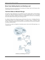
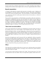
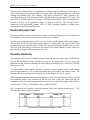
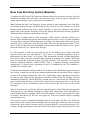
Model Flow Chart
Complete each worksheet row by row from top to bottom by entering values in shaded cells. To
move between worksheets simply "click" on the tabs at the bottom of each screen or on the
"blue-underlined" hyperlinks built into the worksheets. The RETScreen Model Flow Chart is
presented below.
RETScreen Model Flow Chart
BIOH.4
RETScreen® Biomass Heating Project Model
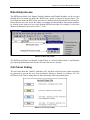
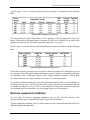
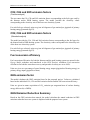
Data & Help Access
The RETScreen Online User Manual, Product Database and Weather Database can be accessed
through the Excel menu bar under the "RETScreen" option, as shown in the next figure. The
icons displayed under the RETScreen menu bar are displayed in the floating RETScreen toolbar.
Hence the user may also access the online user manual, product database and weather database
by clicking on the respective icon in the floating RETScreen toolbar. For example, to access the
online user manual the user clicks on the "?" icon.
RETScreen Menu and Toolbar
The RETScreen Online User Manual, or help feature, is "cursor location sensitive" and therefore
gives the help information related to the cell where the cursor is located.
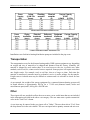
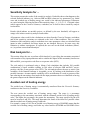
Cell Colour Coding
The user enters data into "shaded" worksheet cells. All other cells that do not require input data
are protected to prevent the user from mistakenly deleting a formula or reference cell. The
RETScreen Cell Colour Coding chart for input and output cells is presented below.
RETScreen Cell Colour Coding
BIOH.5
RETScreen® Software Online User Manual
Currency Options
To perform a RETScreen project analysis, the user may select a currency of their choice from the
"Currency" cell in the Cost Analysis worksheet.
The user selects the currency in which the monetary data of the project will be reported. For
example, if the user selects "$," all monetary related items are expressed in $.
Selecting "User-defined" allows the user to specify
the currency manually by entering a name or
symbol in the additional input cell that appears
adjacent to the currency switch cell. The currency
may be expressed using a maximum of three
characters ($US, £, ¥, etc.). To facilitate the
presentation of monetary data, this selection may
also be used to reduce the monetary data by a factor
(e.g. $ reduced by a factor of a thousand, hence
k$ 1,000 instead of $ 1,000,000).
If "None" is selected, all monetary data are
expressed without units. Hence, where monetary
data is used together with other units (e.g. $/kWh)
the currency code is replaced with a hyphen
(-/kWh).
The user may also select a country to obtain the
International Standard Organisation (ISO) threeletter country currency code. For example, if
Afghanistan is selected from the currency switch
drop-down list, all project monetary data are
expressed in AFA. The first two letters of the
country currency code refer to the name of the
country (AF for Afghanistan), and the third letter to
the name of the currency (A for Afghani).
For information purposes, the user may want to
assign a portion of a project cost item in a second
currency, to account for those costs that must be
paid for in a currency other than the currency in
which the project costs are reported. To assign a
cost item in a second currency, the user must select
the option "Second currency" from the "Cost
references" drop-down list cell.
Some currency symbols may be unclear on the
screen (e.g. €); this is caused by the zoom settings
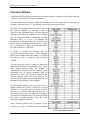
List of Units, Symbols and Prefixes
BIOH.6
RETScreen® Biomass Heating Project Model
of the sheet. The user can increase the zoom to see those symbols correctly. Usually, symbols
will be fully visible on printing even if not fully appearing on the screen display.
Units, Symbols & Prefixes
The previous table presents a list of units, symbols and prefixes that are used in the RETScreen
model.
Note: 1. The gallon (gal) unit used in RETScreen refers to US gallon and not to imperial
gallon.
2. The tonne (t) unit used in RETScreen refers to metric tonnes.
Unit Options
To perform a RETScreen project analysis, the user must choose between "Metric" units or
"Imperial" units from the "Units" drop-down list.
If the user selects "Metric," all input and output values will be expressed in metric units. But if
the user selects "Imperial," input and output values will be expressed in imperial units where
applicable.
Note that if the user switches between "Metric" and
"Imperial," input values will not be automatically converted
into the equivalent selected units. The user must ensure that
values entered in input cells are expressed in the units
shown.
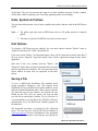
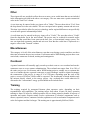
Saving a File
To save a RETScreen Workbook file, standard Excel
saving procedures should be used. The original Excel
Workbook file for each RETScreen model cannot be saved
under its original distribution name. This is done so that the
user does not save-over the "master" file. Instead, the user
should use the "File, Save As" option. The user can then
save the file on a hard drive, diskette, CD, etc. However, it
is recommended to save the files in the "MyFiles" directory
automatically set by the RETScreen installer program on
the hard drive.
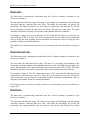
The download procedure is presented in the following
figure. The user may also visit the RETScreen Website at
www.retscreen.net for more information on the download
procedure. It is important to note that the user should not
RETScreen Download Procedure
BIOH.7
RETScreen® Software Online User Manual
change directory names or the file organisation automatically set by RETScreen installer
program. Also, the main RETScreen program file and the other files in the "Program" directory
should not be moved. Otherwise, the user may not be able to access the RETScreen Online User
Manual or the RETScreen Weather and Product Databases.
Printing a File
To print a RETScreen Workbook file, standard Excel printing procedures should be used. The
workbooks have been formatted for printing the worksheets on standard "letter size" paper with a
print quality of 600 dpi. If the printer being used has a different dpi rating then the user must
change the print quality dpi rating by selecting "File, Page Setup, Page and Print Quality" and
then selecting the proper dpi rating for the printer. Otherwise the user may experience quality
problems with the printed worksheets.
BIOH.8
RETScreen® Biomass Heating Project Model
Biomass Heating Project Model
The RETScreen® International Biomass Heating Project Model can be used world-wide to easily
evaluate the energy production (or savings), life-cycle costs and greenhouse gas emissions
reduction for biomass and/or waste heat recovery (WHR) heating projects, ranging in size from
large-scale developments for clusters of buildings to individual building applications. The model
can be used to evaluate three basic heating systems using: waste heat recovery; biomass; and
biomass and waste heat recovery combined. It also allows for a "peak load heating system" to be
included (e.g. oil-fired boiler). The model is designed to analyse a wide range of systems with or
without district heating.
Six worksheets (Energy Model, Heating Load Calculation & District Heating Network Design
(Heating Load & Network), Cost Analysis, Greenhouse Gas Emission Reduction Analysis (GHG
Analysis), Financial Summary and Sensitivity and Risk Analysis (Sensitivity)) are provided in the
Biomass Heating Project Workbook file.
The Energy Model and Heating Load & Network worksheets are completed first. The Cost
Analysis worksheet should then be completed, followed by the Financial Summary worksheet.
The GHG Analysis and Sensitivity worksheets are optional analyses. The GHG Analysis
worksheet is provided to help the user estimate the greenhouse gas (GHG) mitigation potential of
the proposed project. The Sensitivity worksheet is provided to help the user estimate the
sensitivity of important financial indicators in relation to key technical and financial parameters.
In general, the user works from top-down for each of the worksheets. This process can be
repeated several times in order to help optimise the design of the biomass heating project from an
energy use and cost standpoint.
In addition to the worksheets that are required to run the model, the Introduction worksheet and
Blank Worksheets (3) are included in the Biomass Heating Project Workbook file. The
Introduction worksheet provides the user with a quick overview of the model. Blank Worksheets
(3) are provided to allow the user to prepare a customised RETScreen project analysis. For
example, the worksheets can be used to enter more details about the project, to prepare graphs
and to perform a more detailed sensitivity analysis.
BIOH.9
RETScreen® Software Online User Manual
Energy Model
As part of the RETScreen Clean Energy Project Analysis Software, the Energy Model and
Heating Load & Network worksheets are used to help the user calculate the annual energy
production for a biomass and/or WHR heating project based upon local site conditions and
system characteristics. Results are calculated in common megawatt-hour (MWh) units for easy
comparison of different technologies.
Site Conditions
The site conditions associated with estimating the annual energy production of a biomass and/or
WHR heating project are detailed below.
Project name
The user-defined project name is given for reference purposes only.
For more information on how to use the RETScreen Online User Manual, Product Database and
Weather Database, see Data & Help Access.
Project location
The user-defined project location is given for reference purposes only.
Nearest location for weather data
The user enters the weather station location in the Heating Load & Network worksheet and it is
copied automatically to the Energy Model worksheet.
Note: At this point the user should complete the Heating Load & Network worksheet.
Number of buildings
The model calculates the total number of buildings from data entered by the user in the Heating
Load & Network worksheet.
Total pipe length
The model calculates the total pipe length from data entered in the Heating Load & Network
worksheet. The total pipe length is equal to the sum of "Total pipe length for main distribution
line" and "Length of pipe section" for the secondary distribution line length. Total pipe length is
equal to trench length (the trench contains both supply and return lines).
BIOH.10
RETScreen® Biomass Heating Project Model
Heating energy demand
The model calculates the heating energy demand from the data entered in the Heating Load &
Network worksheet.
Units switch: The user can choose to express the energy in different units by selecting among
the proposed set of units: "GWh," "Gcal," "million Btu," "GJ," "therm," "kWh," "hp-h," "MJ."
This value is for reference purposes only and is not required to run the model.
Peak heating load
The model calculates the peak heating load from data entered in the Heating Load & Network
worksheet.
Units switch: The user can choose to express the load in different units by selecting among the
proposed set of units: "MW," "million Btu/h," "boiler hp," "ton (cooling)," "hp," "W." This value
is for reference purposes only and is not required to run the model.
System Characteristics
The model can evaluate heating system designs consisting of waste heat recovery and various
boiler types:
1. Waste heat recovery (WHR) system;
2. Biomass heating system;
3. Peak load heating system designed to meet a small portion of the annual energy demand
during peak heating periods; and
4. Back-up heating system (optional), which is used in case of system shutdown or because
of an interruption in the waste heat recovery system or biomass fuel supply.
The system characteristics associated with estimating the annual energy production of a biomass
and/or WHR heating project are detailed below. The system characteristics are divided into four
sub-sections: Waste Heat Recovery System, Biomass Heating System; Peak Load Heating
System; and, Back-up Heating System.
System type
The user selects the type of base load heating system considered from the three options in the
drop-down list: "WHR" (waste heat recovery system), "Biomass" (biomass heating system) and
"Biomass & WHR" (biomass heating system and waste heat recovery (WHR) combined).
BIOH.11
RETScreen® Software Online User Manual
The model assumes that the system type selected will provide the base load heating energy
demand with the peak load system meeting the remaining energy demand not met by the base
load system. Within the base load system the model assumes that the full amount of energy
available from the WHR system will be used before energy is supplied by the biomass heating
system.
The "System Design Graph" provided summarises essential design information for the user. For
example, the stacked bar chart on the left shows the percentage of the installed heating power
capacity for each of the heating systems (WHR, biomass and peak) with respect to the peak
heating load. The bar chart can exceed 100% to allow the system to be oversized. The stacked
bar chart on the right shows the percentage of total heating energy demand supplied by each of
the heating systems. The bar chart cannot exceed 100%.
Waste Heat Recovery (WHR) System
Waste heat is available from many sources. The model does not distinguish the origin of the heat.
Waste heat is assumed to be available at all times and is considered base load for the energy
calculations.
Typical sources of waste heat are heat recovered from a process or cooling of a machine.
Electricity generating systems are often used. For example, with a reciprocating engine that
produces electricity, the jacket and lubrication cooling in combination with exhaust gas cooling
can recover heat equal to the shaft power.
Waste heat recovery system capacity
The user enters the waste heat recovery system capacity available, in kW. This value is
transferred to the Cost Analysis worksheet. For example, a 500 kW diesel electric generator used
in a base load mode will provide approximately 500 kW of WHR capacity. Use the "System
Design Graph" (as displayed in the Energy Model worksheet) as a guide.
Waste energy delivered
The model calculates the waste energy delivered, in MWh. The waste energy delivered is the
annual energy production provided by the WHR system.
Percentage of peak heating load
The model calculates the percentage of the WHR system installed capacity with respect to the
peak heating load.
Percentage of total heating energy demand
The model calculates the percentage of total heating energy demand supplied by the WHR
system.
BIOH.12
RETScreen® Biomass Heating Project Model
Biomass Heating System
Biomass is available in many forms. The model is designed to evaluate the energy available from
any biomass source. It should be noted that the most successful biomass heating systems use a
consistent fuel. The fuel can be a mixture of fuel types, size distribution and moisture content as
long as the mixture stays constant. When the fuel changes the system might require manual retuning to achieve full efficiency and minimize emissions.
Biomass fuel type
The user selects the biomass fuel type from the drop-down list. If the fuel available is not listed,
select a fuel that has a similar heating value as found in the table below. The heating value listed
is the higher heat value on a dry basis.
Biomass Fuel Type and Corresponding Heating Value
The heating value can change depending on its origin. Typically wood bark has a higher heating
value then the white wood. The heating value is also reduced over time from harvesting.
Moisture content on wet basis of biomass
The user enters the moisture content on wet basis of the biomass to be fed into the biomass
system.
Typical values for moisture content of wood range from 10 to 50%. Freshly chipped wood
averages from 40 to 55% moisture content. Fuel dried until it reaches a moisture content of
30 to 40% is ideal for most small-commercial burners [Sykes, 1997]. For wood fuels, moisture
content is normally expressed on a wet basis. In some cases, information of moisture content on
a dry basis, instead of on a wet basis, may be available to the user and the following conversion
should be applied: moisture content wet basis = moisture content dry basis/(1 + moisture content
dry basis).
Typically fuels that have a moisture content above 50 to 55% require drying before they can be
used as a fuel.
BIOH.13
RETScreen® Software Online User Manual
As-fired heating value of biomass
The model calculates the as-fired heating value of biomass using the biomass dry heating value
and the moisture content. The as-fired heating value of biomass is the energy content of 1 tonne
of the particular fuel type on a wet basis. This value is used to calculate the biomass annual fuel
requirement for the system. Typical values for moist heating value for biomass range from
10,800 to 15,900 MJ/tonne. The lower the moisture content, the higher the heating value of the
biomass fuel [Hayden, 1997].
Biomass boiler(s) capacity (# boilers)
The user enters the biomass boiler capacity. The model assumes that the capacity is the energy
output of the biomass boiler as biomass energy systems are typically rated on output. Use the
"System Design Graph" (as displayed in the Energy Model worksheet) as a guide. This value is
transferred to the Cost Analysis worksheet. If more than one biomass boiler is proposed, then the
value entered is the sum of the biomass boiler capacities. The user can consult the RETScreen
Online Product Database for more information, or to change the number of boilers shown.
Biomass boiler(s) manufacturer
The user enters the name of the biomass boiler(s) manufacturer for reference purposes only. The
user can consult the RETScreen Online Product Database for more information.
Biomass boiler(s) model
The user enters the name of the biomass boiler(s) model for reference purposes only. The user
can consult the RETScreen Online Product Database for more information.
Biomass boiler(s) seasonal efficiency
The user enters the biomass boiler seasonal efficiency. This value is generally lower than the
steady-state efficiency because it is calculated on a seasonal basis. In other words, the "steadystate efficiency" is for full load conditions while the "seasonal efficiency" takes into
consideration the lower efficiency part load conditions that occur during the year. The seasonal
efficiency is also related to the particular boiler chosen and the operating temperature of the
system. This value is used to estimate the biomass fuel requirement to meet the biomass system
energy demand. Typical values for seasonal efficiency of a biomass boiler range from 60 to 90%.
The seasonal efficiency is typically higher for two-burner systems than a one-burner system. The
user can consult the RETScreen Online Product Database for more information.
BIOH.14
RETScreen® Biomass Heating Project Model
Biomass energy delivered
The model calculates the biomass energy delivered, in MWh. The biomass energy delivered is
the annual energy production provided by the biomass heating system.
Percentage of peak heating load
The model calculates the percentage of the installed capacity of the biomass heating system with
respect to the peak heating load.
Percentage of total heating energy demand
The model calculates the percentage of total heating energy demand supplied by the biomass
heating system.
Peak Load Heating System
Peak load system fuel type
The user selects the peak load heating system fuel type from the drop-down list. The user can
also choose a "biomass" peak load heating system. The model then assumes that the biomass fuel
type is the same chosen under "Biomass fuel type" in the section above. For more information on
the default heating values used for each peak load system fuel type see Unit cost of fuel.
Peak load system steady-state efficiency
The user enters the peak load steady-state efficiency. This value is used to calculate the
suggested peak load system capacity. Use the "System Design Graph" (as displayed in the
Energy Model worksheet) as a guide. Typical values for steady-state efficiency of a peak heating
system range from 50 to 350% [Hayden, 1997] (efficiencies above 100% can occur when, for
instance, the peak heating system is a heat pump). The peak load steady-state efficiency varies
depending on altitude, heating system type, design temperatures, etc. Set the peak load steadystate efficiency to 100% if boilers are rated on an output basis rather than on a heating value
input basis.
Suggested peak load system capacity
The model calculates the suggested peak load boiler capacity required to meet the heating load as
set by the design requirements established above. This value is calculated by subtracting the
WHR (if included) system capacity and the biomass boiler capacity from the peak heating load.
BIOH.15
RETScreen® Software Online User Manual
Peak load system capacity
The user enters the peak load system capacity. If the capacity is below the suggested peak load
system capacity the system cannot meet the peak heating load at design conditions. Use the
"System Design Graph" (as displayed in the Energy Model worksheet) as a guide. This value is
transferred to the Cost Analysis worksheet.
Peak load system seasonal efficiency
The user enters the peak load system seasonal efficiency. This value is generally lower than the
steady-state efficiency because it is calculated on a seasonal basis. This value is used to estimate
the peak load fuel requirement to meet the peak load heating system energy demand. Typical
values for seasonal efficiency for peak load heating systems range from 55 to 350%. Typical
values of heating system efficiency are presented below.
Typical Heating System Seasonal Efficiencies
Suggested biomass boiler capacity
The model calculates the suggested biomass boiler capacity required to meet the peak heating
load as set by the design requirements established above. This value is calculated by subtracting
the WHR (if included) system capacity and the base load biomass boiler capacity from the peak
heating load.
Biomass boiler capacity
The user enters the peak load biomass boiler capacity. The model assumes that the capacity is the
energy output of the biomass boiler as biomass energy systems are typically rated on output. Use
the "System Design Graph" (as displayed in the Energy Model worksheet) as a guide. This value
is transferred to the Cost Analysis worksheet. The user can consult the RETScreen Online
Product Database for more information.
BIOH.16
RETScreen® Biomass Heating Project Model
Biomass boiler seasonal efficiency
The user enters the peak load biomass boiler seasonal efficiency. This value is generally lower
than the steady-state efficiency because it is calculated on a seasonal basis. In other words, the
"steady-state efficiency" is for full load conditions while the "seasonal efficiency" takes into
consideration the lower efficiency part load conditions that occur during the year. The seasonal
efficiency is also related to the particular boiler chosen and the operating temperature of the
system. This value is used to estimate the biomass fuel requirement to meet the peak load
biomass system energy demand. Typical values for seasonal efficiency of a biomass boiler range
from 60 to 90%. The seasonal efficiency is typically higher for two-burner systems than a oneburner system. The user can consult the RETScreen Online Product Database for more
information.
Peak energy delivered
The model calculates the peak energy delivered, in MWh. The peak energy delivered is the
annual energy production provided by the peak load heating system.
Percentage of peak heating load
The model calculates the percentage of the installed capacity of the peak load heating system
with respect to the peak heating load.
Percentage of total heating energy demand
The model calculates the percentage of total heating energy demand supplied by the peak load
heating system. The model assumes that the WHR system is used in base load mode, with the
biomass system taking second priority. If a WHR system is not included in the design, the model
assumes that the biomass heating system is used in base load mode. In each case the model
assumes that energy is supplied by the peak load heating system only after all the energy is first
supplied by the WHR system and/or the biomass heating system - in regards to the peak heating
load and total heating energy demand.
Back-up Heating System (optional)
Suggested back-up heating system capacity
Back-up heating system capability may be part of a district heating system. A common "rule-ofthumb" is that each heating plant should have back-up capability equal to the largest unit on the
system [Arkay, 1996]. For example, a back-up boiler may be utilised in the case of a boiler
shutdown or during an interruption in the biomass fuel supply. The model calculates the largest
unit capacity by comparing the sizes of the base load and the peak load heating systems. For new
construction projects, a new oil-fired back-up boiler is likely purchased. For retrofit situations,
the existing oil-fired heating system may be used as a back-up. The use of a back-up heating
BIOH.17
RETScreen® Software Online User Manual
system depends on the "design philosophy" of the user. The back-up heating system provides
greater security, but at a higher cost in new systems. A used oil boiler will often suffice as a
back-up unit. In other cases a designer may choose not to include a back-up unit, rather relying
only on the peak load boiler
Back-up heating system capacity
The user enters the back-up heating system capacity according to the back-up heating system
capacities available on the market, or available in a retrofit situation, and the suggested back-up
heating system capacity. This value may be used in the Cost Analysis worksheet if a back-up
system is used.
Annual Energy Production
Items associated with calculating the annual energy production and fuel required of the biomass
and/or WHR heating project are detailed below.
Percentage of peak heating load
The model calculates the percentage of the installed capacity of the system type specified by the
user with respect to the peak heating load.
Heating capacity
The heating system heating capacities entered by the user are summarised here.
Units switch: The user can choose to express the capacity in different units by selecting among
the proposed set of units: "MW," "million Btu/h," "boiler hp," "ton (cooling)," "hp," "W." This
value is for reference purposes only and is not required to run the model.
Equivalent full output hours
The model calculates the equivalent full output hours of the WHR, biomass and peak load
heating systems.
Capacity factor
The model calculates the capacity factor of the WHR, biomass and peak load heating systems,
which is the annual energy production of the these systems expressed as a percentage of their
potential energy output if used at rated capacity continuously over a one year period.
BIOH.18
RETScreen® Biomass Heating Project Model
Percentage of total heating energy demand
The model calculates the percentage of total heating energy demand supplied by the system type
specified by the user.
Heating energy delivered
The model calculates the heating energy delivered by the system type specified by the user.
Units switch: The user can choose to express the energy in different units by selecting among
the proposed set of units: "GWh," "Gcal," "million Btu," "GJ," "therm," "kWh," "hp-h," "MJ."
This value is for reference purposes only and is not required to run the model.
Biomass requirement
The model calculates the biomass requirement. This value is the amount of biomass fuel,
expressed in wet (as-fired) metric tonnes per year, consumed by the biomass heating system in
order to meet the specified biomass heating system annual energy production. This output value
is calculated using the annual energy delivered of the biomass system, the as-fired heating value
of biomass and the biomass boiler seasonal efficiency. The value is transferred to the Cost
Analysis worksheet.
Heating fuel requirement
The model calculates the heating fuel requirement, expressed in units as shown per year,
consumed by the peak load heating system. This value is transferred to the Cost Analysis
worksheet.
BIOH.19
RETScreen® Software Online User Manual
Heating Load Calculation & District Heating Network Design
As part of the RETScreen Clean Energy Project Analysis Software, the Heating Load
Calculation & District Heating Network Design worksheet is used in conjunction with the
Energy Model worksheet to estimate the heating load for the proposed biomass and/or WHR
heating system. This worksheet is also used to prepare a preliminary design and cost estimate for
the district heating network. The user should return to the Energy Model worksheet after
completing this section.
Site Conditions
Nearest location for weather data
The user enters the weather station location with the most representative weather conditions for
the project. This is for reference purposes only. The user can consult the RETScreen Online
Weather Database for more information.
Heating design temperature
The user enters the heating design temperature, which represents the minimum temperature that
has been measured for a frequency level of at least 1% over the year, for a specific area
[ASHRAE, 1997]. The design temperature is used to determine the heating energy demand. The
user can consult the RETScreen Online Weather Database for more information.
Typical values for heating design temperature range from approximately -40 to 15°C.
Note: The heating design temperature values found in the RETScreen Online Weather Database
were calculated based on hourly data for 12 months of the year. The user might want to
overwrite this value depending on local conditions. For example, where temperatures are
measured at airports, the heating design temperature could be 1 to 2ºC milder in core areas of
large cities.
The user should be aware that when modifying the design temperature, the monthly degree-days
and the heating load for building cluster might have to be adjusted accordingly.
Annual heating degree-days below 18°C
The model calculates the total annual heating degree-days below 18ºC by summing the monthly
degree-days entered by the user. Degree-days for a given day represent the number of Celsius
degrees that the mean temperature is above or below a given base. Thus, heating degree-days are
the number of degrees below 18ºC. The user can consult the RETScreen Online Weather
Database for more information.
BIOH.20
RETScreen® Biomass Heating Project Model
Domestic hot water heating base demand
The user enters the estimated domestic hot water heating base demand as a percentage of the
annual heating energy demand. To simulate non-weather dependent process demands, the
percentage of domestic hot water base demand can be varied.
Typical values for domestic hot water heating base demand range from 10 to 25%. As an
example, a hospital will probably use 25% of its heating energy to heat domestic hot water while
a regular office building may use only 10% of its heating energy to heat domestic water. If no
domestic water heating is required the user will enter 0.
Equivalent degree-days for DHW heating
The model calculates the equivalent degree-days for DHW heating. While building heating is
often calculated from climatic normals which are expressed in degree-days, the domestic hot
water heating load is often expressed in degree-days/day.
Typical values for equivalent degree-days in DHW heating range from 2 to 10 degree-days/day.
A low hot water heating requirement is equivalent to 2 degree-days/day while a high hot water
heating requirement (e.g. hospital) is equivalent to 6 to 10 degree-days/day. If there is no need
for hot water heating the value 0 is calculated by the model.
Equivalent full load hours
The model calculates the equivalent full load hours, which is defined as the annual energy
demand divided by the total peak heating load for a specific location. This value is expressed in
hours and is equivalent to the number of hours that a heating system sized exactly for the peak
heating load would operate at rated capacity to meet the annual heating energy demand. The
typical values for the equivalent full load hours is in the range from 1,500 to 4,200 hours. The
upper range increases if the system has a high domestic hot water load or process load.
Monthly Inputs
The user enters the monthly degree-days below 18ºC. The monthly degree-days are the sum of
the degree-days for each day of the month. Degree-days for a given day represent the number of
Celsius degrees that the mean temperature is above or below a given base. Thus, heating degreedays are the number of degrees below 18ºC. The user can consult the RETScreen Online
Weather Database for more information.
BIOH.21
RETScreen® Software Online User Manual
Base Case Heating System and Heating Load
The system characteristics associated with estimating the heating load for the biomass and/or
WHR heating system are detailed below.
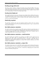
Technical Note on Network Design
The purpose of this technical note is to provide the user with a sample design of a district heating
network used within the RETScreen model. The example described below refers to the default
values that come with the "BIOH3.xls" RETScreen workbook file for the base case and heating
load section and the district heating network design section.
In a district heating system, thermal energy, in the form of hot water, is distributed from the
central heating plant to the individual buildings. The thermal energy is distributed using
networks of insulated underground arterial pipeline (main distribution line) and branch pipelines
(secondary distribution lines).
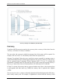
The network can either be designed as a branched system as shown in the following figure, or as
a looped system.
Community System Building Cluster Layout
BIOH.22
RETScreen® Biomass Heating Project Model
The previous figure shows how the different building clusters are connected to the main
distribution line (i.e. section 1, 2, etc.). Note that the office building (cluster 4) and the apartment
building (cluster 5) are not put in the same building cluster as they have different heating loads.
If they are put together the secondary pipe size will be incorrect. The following table provides a
summary of the heating loads and pipe lengths for the building clusters shown in the previous
figure.
Community System Base Case Heating System and Heating Load
Base Case Heating System
Heated floor area per building cluster
The user enters the total heated floor area for the building(s) in a cluster. A building cluster is
any number of similar buildings connected to a single point of the distribution system. The
heated floor area per building cluster is the floor surface area of the building(s) that have to be
heated, multiplied by the number of floors. The user obtains this value for each of the buildings
included in the biomass and/or WHR heating system and summarises the values to enter the
cluster total heating surface area (See Technical Note on Network Design ).
Typical values for total floor heating surface area range from 500 to 9,000 m². Most commercial
or institutional buildings will have a heating surface exceeding 500 m². A typical value of
heating surface area for an individual house is 140 m².
Note: When the user enters 0 or leaves the heated floor area per building cluster cell blank, the
remaining column in this section is greyed out.
BIOH.23
RETScreen® Software Online User Manual
Number of buildings in building cluster
The user enters the number of buildings in each building cluster.
Heating fuel type(s)
The user selects the type of fuel that is used to heat the cluster of buildings. A list of common
fuels is provided in the drop-down list.
The following table provides the heating value for the heating energy avoided.
Fuel Heating Content
Note: Propane is expressed in terms of liquefied propane.
Heating system seasonal efficiency
The user enters the average efficiency of the conventional heating system over the season of use.
This entry is used to calculate the financial value of the system. It has no influence on the
calculation of the annual energy production. Typical values range from 55% for conventional
fossil-fuel-fired heaters to 100% for electric heaters. If a heat-pump is used as a base case the
user will select "Electricity" as the heating fuel type and may enter values higher than 100% to
reflect the heat pump coefficient of performance (COP) (e.g. enter 225% if seasonal COP is
2.25).
Typical values of heating system efficiency are presented in the table below. These values should
be reduced by 10% if ducting runs outside of the insulated envelope (e.g. in attics).
Typical Heating System Seasonal Efficiencies
BIOH.24
RETScreen® Biomass Heating Project Model
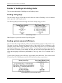
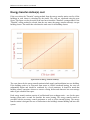
Heating Load Calculation
Heating load for building cluster
The user enters the heating load for building cluster. The user can refer to the next figure
[CET, 1997] to estimate the building heating load per unit of building heating surface area. This
value depends on the design temperature for the specific location and on the building insulation
efficiency. The heating load for building cluster is used to calculate the peak heating load for the
heating system. Typical values for building heating load range from 40 to 120 W/m².
Building Heating Load Chart
Note: The values in this figure are more appropriate for residential buildings.
Heating energy demand
The model calculates the buildings cluster's annual heating energy demand, which is the amount
of energy required to heat the building(s) in the building cluster (including domestic hot water).
BIOH.25
RETScreen® Software Online User Manual
This value is calculated from the heated floor area per building cluster, the heating load for
building cluster and the equivalent full load hours.
Total peak heating load
The model calculates the building cluster's total peak heating load, which is the heating power
required to meet the largest heating load for the year. It typically coincides with the coldest day
of the year. This value is transferred to the Energy Model worksheet.
Fuel consumption - units
The model displays the units used for the heating fuel type selected for each building cluster.
Note that the fuel consumption unit for propane is litres of liquefied propane.
Fuel consumption - annual
The model calculates the annual fuel consumption for each building cluster. If the fuel
consumption is known for the building(s) this row can be used to determine the "Heating load for
building cluster." For example, the user may know (from previous years heating bills) how many
litres of heating oil are purchased. In this case the user would vary the "Heating load for building
cluster" value until the fuel consumption value converges to the value shown on their heating
bills.
Cost of fuel - units
The model displays the units used for the heating fuel type selected for each building cluster.
Note that the cost of fuel unit for propane is expressed in terms of litres of liquefied propane.
Unit cost of fuel
The user enters the unit cost of the heating fuel type selected for each building cluster. The user
is given the flexibility in the model to determine what is the "conventional," or base case, energy
system. The user will need to determine this value according to the cost units given in the table.
Heating values are also given in the table below.
Energy Cost Unit and Heating Content (Energy Mines and Resources Canada, 1985)
BIOH.26
RETScreen® Biomass Heating Project Model
Note that the cost unit of propane is expressed in terms of litres of liquefied propane. The unit
cost of fuel is used in conjunction with the total heating energy demand, the heating value and
the base case heating system seasonal efficiency to calculate the total fuel cost.
In cases when the heating energy avoided is electricity, the user will normally enter the retail
price of electricity as the unit cost of fuel. Note that the heating value for the "Other" type of
heating energy avoided has been set to 1.0. This implies that the user must enter the cost in terms
of $ per MWh of heating energy content of the fuel considered.
Total fuel cost
The model calculates the total fuel cost for each building cluster.
District Heating Network Design
This section is used to prepare a preliminary design and cost estimate for the district heating
network.
Small-commercial biomass and/or WHR heating systems usually use 32 to 150 mm (1 ½ to 6")
diameter treated plastic or steel-in-plastic insulated pipes for heat distribution. These pipes have
proven to be economical to purchase, install, and maintain, but require water temperatures of less
than 130°C (95°C for plastic pipes). The pipe diameter varies depending on the heating load of
the system. When pipe length is used in this section it refers to trench length (with two pipes).
The heat losses for a district heating system vary depending on many factors. For example, an
area with snow cover for a long period has fewer losses than an area with similar temperatures
and no snow cover. In the RETScreen Biomass Heating model, heat losses have not been
included as a separate line item. The annual heat losses for a modern district heating system are
in the range of 2 to 3% of all delivered energy. These numbers change if the pipe length is short
and delivered energy is high.
As an example, the heat loss is approximately 58 W/m for a two-pipe system of a DN125 pipes
using an average annual supply temperature of 100°C and an average annual return temperature
of 50°C. The capacity is 3,400 kW for a DN125 pipe assuming a temperature difference of 45°C.
Additional information may be obtained from the District Heating Handbook [Randløv, 1997].
Design Criteria
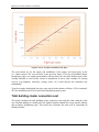
Design supply temperature
The user enters the design supply temperature for the district heating network. Typically plastic
pipes are smaller than DN100 (100 mm or 4") and have a maximum temperature rating of 95°C;
steel pipes are typically rated up to 130°C. If a mixed (plastic and steel) system is designed the
rating for the plastic pipes governs the maximum water temperature allowable. A minimum
supply temperature of 70°C is typically required for supplying heat to domestic hot water.
BIOH.27
RETScreen® Software Online User Manual
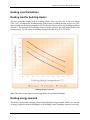
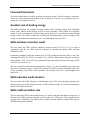
The next figure illustrates typical district heating temperatures in relation to ambient
temperature. Medium Temperature (MT) supply is typical for steel pipe systems. Low
Temperature (LT) supply is typical for plastic pipe or mixed type systems. MT return is typical
for district heating systems with a mixture of old and new buildings. LT return represents a
system with buildings specifically designed for district heating and optimisation of the return
temperature. (High temperature district heating systems are very rare and typically use supply
temperatures that are well above temperatures shown in the following figure - i.e. about 150°C).
Typical District Heating Supply and Return Temperatures
Design return temperature
The user enters the design return temperature for the district heating network. A low return
temperature is desirable. Lower return temperatures makes it possible to reduce pipe sizes and
achieve higher efficiencies for waste heat recovery. For older buildings the winter return
temperature is likely to be around 75°C. For new systems designed to minimise the return
temperature, 50°C can be achieved. (See the Typical District Heating Supply and Return
Temperatures graph for more information.)
BIOH.28
RETScreen® Biomass Heating Project Model
Differential temperature
The model calculates the differential temperature from the difference between design supply and
return temperatures. This value is used to calculate the size of the district heating pipes.
Main Distribution Line
The main distribution line is the part of the district heating pipe system that connects several
buildings, or clusters of buildings, to the heating plant. The first section exiting the heating plant
typically has the largest pipe diameter as it has to serve all the buildings. The pipe diameter is
reduced as the load decreases farther away from the heating plant. The type of pipe can change
from steel to plastic if the system is designed as a low temperature supply system (i.e. below
95°C).
Note: If the system consists of only one building connected to the heating plant, this pipe is
considered to be a secondary line.
Main pipe network oversizing
The user enters a pipe network oversizing factor. The selected pipe sizes are then automatically
sized for a load that is increased by the oversizing factor entered by the user. Pipe oversizing is
used if it is expected that the system load will increase in the future.
For example, if a community studied requires a 500 kW heating system, but there is a plan to add
additional housing that would require an additional load of 50 kW, an oversizing factor of 10%
would ensure that the new housing can be connected at a later date. The oversizing factor is also
used to test how much extra load the selected system can accommodate. This is achieved by
changing the factor until the pipe size is increased. If the pipe sizes change when the oversizing
factor is 15% this indicates that the selected system can handle 15% more load without having to
change the size of the pipes.
Pipe sections
The user indicates by selecting from the drop-down list whether or not a building cluster is
connected to a section of the main distribution line. The user also specifies the length of each
section of the main distribution line. The model then calculates the total load connected to the
section and selects the pipe size. For more information, see example in Technical Note on
Network Design.
The selection of pipe size for this model uses a simplified method. The pipe sizing criteria used
allows a pressure drop for the maximum flow between 1 to 2 millibar per meter. The maximum
velocity in larger pipes is maximised to 3 m/s. Before construction it is necessary to verify that
the selected pipe system will be able to withstand all relevant actions and fulfil the safety and
functional requirements during its entire service life. The final pipe size needs to be verified
BIOH.29
RETScreen® Software Online User Manual
using detailed calculations including pipe length and factor in the number of valves, connection
points, elbows, etc.
Total pipe length for main distribution line
The model calculates the total pipe length for the main distribution network.
Secondary Distribution Lines
The secondary distribution lines are the part of the district heating pipe system that connects
individual buildings to the main distribution line. If the system consists only of one building
connected to the heating plant, this pipe is considered a secondary line.
Secondary pipe network oversizing
The user enters a pipe network oversizing factor. The selected pipe sizes are then automatically
sized for a load that is increased by the oversizing factor entered by the user. Pipe oversizing is
used if it is expected that the system load will increase in the future.
For example, if a community studied requires a 500 kW heating system, but there is a plan to add
additional housing that would require an additional load of 50 kW, an oversizing factor of 10%
would ensure that the new housing can be connected at a later date. The oversizing factor is also
used to test how much extra load the selected system can accommodate. This is achieved by
changing the factor until the pipe size is increased. If the pipe sizes change when the oversizing
factor is 15% this indicates that the selected system can handle 15% more load without having to
change the size of the pipes.
Secondary network pipes are not oversized if, for example, the new buildings that are intended to
be connected in the future will be independent of the existing secondary lines.
Length of pipe section
The user enters the length of each building cluster section of the secondary distribution line. In a
cluster of buildings of the same size, the user should insert the total length of pipe used to
connect to the main distribution line. For more information, see Technical Note on Network
Design.
Pipe size
The model calculates the pipe size for each building load of the building cluster. Note that the
pipe size is selected using the oversizing factor.
The selection of pipe size for this model uses a simplified method. The pipe sizing criteria used
allows a pressure drop for the maximum flow between 1 to 2 millibar per meter. The maximum
velocity in larger pipes is maximised to 3 m/s. Before construction it is necessary to verify that
BIOH.30
RETScreen® Biomass Heating Project Model
the selected pipe system will be able to withstand all relevant actions and fulfil the safety and
functional requirements during its entire service life. The final pipe size needs to be verified
using detailed calculations including pipe length and factor in the number of valves, connection
points, elbows, etc.
District Heating Network Costs
In this section two alternative methods are provided for assessing the costs for district heating
pipes and energy transfer stations - Formula costing and Detailed costing.
Total pipe length
The model calculates the total pipe length as the sum of the total pipe length for the main
distribution line and the total pipe length for the secondary distribution lines.
Costing method
The user selects the type of costing method. The options from the drop-down list are: "Formula"
and "Detailed." If the formula method is selected, the model calculates the costs according to
built-in formulas. If the detailed method is selected, the user enters the Energy Transfert Station
(ETS) and secondary distribution pipes costs per building cluster and the main distribution line
pipe cost by pipe size categories.
The costs calculated by the formula method are based on typical Canadian project costs as of
January 2000. The user can adjust these costs to local conditions using the cost factors in the
cells below and by the "Exchange rate" cell.
Energy transfer station(s) connection type
The user selects the energy transfer connection type from the two options in the drop-down list:
"Direct" and "Indirect." If "Direct" is selected, the model sets the costs for energy transfer
stations to $0. If "Indirect" is selected, the model calculates the costs according to built-in
formulas if "Formula" costing method is selected, or the user enters these costs if "Detailed"
costing method is chosen.
The building's heating system is normally connected indirectly to the district heating system via
energy transfer stations located in the basement or where a boiler would normally be located.
Direct systems connect the district heating system directly to the building's heating system.
Energy transfer station(s) cost factor
If the user selects the "Formula" costing method, then an energy transfer station cost factor can
be entered. This factor is used to modify the built-in formula to compensate for local variations
in construction costs, inflation, etc.
BIOH.31
RETScreen® Software Online User Manual
Energy transfer station(s) cost
If the user selects the "Formula" costing method, then the energy transfer station cost for all the
buildings in each cluster is calculated by the model. The costs are calculated using the next
figure. This figure can also be useful if the user has selected the "Detailed" costing method. If the
"Detailed" costing method is selected, then the user enters the energy transfer station(s) cost per
building cluster. The model then calculates the total costs for all building clusters.
Typical Costs for Energy Transfer Station(s)
The costs shown for the energy transfer station include supply and installation in a new building.
If the building needs to be converted from steam or electric baseboard heating, the costs are
substantially higher and should be confirmed by a local contractor. It should be noted that
building owners sometimes choose to remove existing boilers and domestic hot water storage
tanks to gain valuable floor space.
Each energy transfer station consists of prefabricated heat exchanger units - one for the space
heating system and a second for domestic hot water heating. The energy transfer station is
provided with the necessary control equipment as well as all the internal piping. The energy
transfer station is designed for ease of connection to the building's internal heating and hot water
system.
BIOH.32
RETScreen® Biomass Heating Project Model
Domestic hot water tanks and boilers are typically replaced with only a heat exchanger. Where
the domestic hot water consumption is large, storage tanks can be used.
Typically, each building includes an energy meter. These meters record district heating water
flow through the energy transfer station. By measuring the temperature difference of incoming
and return water temperature, the energy usage is calculated.
Prefabricated energy transfer stations with heat exchanger units for both heating and domestic
hot water are available for single-family residences and small multi-family residences. They
consist of brazed plate or "shell and tube" heat exchangers for both heating and domestic hot
water, a circulation pump, an expansion tank, self-actuating control valves and an energy meter.
For larger buildings, the energy transfer station will be site assembled but will consist of the
equipment with the same functions as for smaller buildings.
Secondary distribution line pipe cost factor
If the user selects the "Formula" costing method, the secondary distribution line pipe cost factor
can be entered. This factor is used to modify the built-in formula to compensate for local
variations in construction costs, inflation, etc.
Exchange rate
The user enters the exchange rate to convert the calculated Canadian dollar costs into the
currency in which the project costs will be reported. The rate entered must be the value of one
Canadian dollar expressed in the currency in which the project costs will be reported.
Note: The user should first select the currency at the top of the Cost Analysis worksheet.
Secondary distribution line pipe cost
If the user selects the "Formula" costing method, then the secondary distribution line pipe costs
for all pipes connecting each cluster to the main distribution pipe are calculated by the model.
The costs are calculated using the next figure. This figure can also be useful if the user has
selected the "Detailed" costing method. If the "Detailed" costing method is selected, then the
user enters the total cost for the secondary distribution pipes cost per building cluster. The model
then calculates the total costs for all building clusters.
BIOH.33
RETScreen® Software Online User Manual
Typical Costs for Secondary Distribution Line Pipes
The costs shown are for the supply and installation of the supply and return pipes in the
(i.e. 2 pipes) trench. The cost per meter in the previous figure is for two pre-insulated district
heating type pipes, in a trench approximately 600 mm deep; the costs also include repair of the
existing sidewalk or road. Rocky terrain or installations in areas with a number of existing
services (e.g. telephone, electricity, sewage, water, etc.) could increase the calculated cost
substantially.
Typical secondary distribution line pipe costs can be broken down as follows: 45% for material,
45% for installation and 10% for associated distribution pump system.
Total building cluster connection cost
The model calculates the total building cluster connection cost using the values entered by the
user (detailed method) or calculated by the model (formula method) for energy transfer stations
and secondary distribution pipes. The model also calculates the total cost of connecting all
building clusters.
BIOH.34
RETScreen® Biomass Heating Project Model
Main distribution line pipe cost factor
If the user selects the "Formula" costing method, then a main distribution line pipe cost factor
can be entered. This factor is used to modify the built-in formula to compensate for local
variations in construction costs, inflation, etc.
Summary of main distribution line pipe size
The model summarises the pipe sizes specified in the main distribution line sizing section.
Summary of main distribution line pipe length
The model calculates the total length of the main pipe for each pipe diameter.
Summary of main distribution line pipe cost
If the user selects the "Formula" costing method, then the main distribution line pipe cost for all
main pipe sections is calculated by the model. The costs are calculated using the same formula as
for secondary distribution line pipe costs (see the Typical Costs for Secondary Distribution Line
Pipes graph).
If the "Detailed" costing method is selected, then the user enters the total cost for the main
distribution line pipe cost for each pipe size categories. The model calculates the total costs for
all the main distribution pipe costs.
The costs shown are for the supply and installation of two pipes per meter of trench. The cost per
meter is for two pre-insulated district heating type pipes, in a trench approximately 600 mm
deep; the costs also include restoration of the existing sidewalk or road. Rocky terrain or
installation in areas that have many old utility services (e.g. telephone, electricity, sewage, water,
etc.) could substantially increase the quoted costs.
Typical main distribution line pipe costs can be broken down as follows: 45% for material, 45%
for installation and 10% for associated distribution pump system.
Total district heating network costs
The model calculates the total district heating network costs, which include the total cost of
secondary and main distribution pipes plus the total cost of the energy transfer station(s).
Note: The user should return to the Energy Model worksheet.
BIOH.35
RETScreen® Software Online User Manual
Cost Analysis 1
As part of the RETScreen Clean Energy Project Analysis Software, the Cost Analysis worksheet
is used to help the user estimate costs associated with a biomass and/or WHR heating project.
These costs are addressed from the initial, or investment, cost standpoint and from the annual, or
recurring, cost standpoint. The user may refer to the RETScreen Online Product Database for
supplier contact information in order to obtain prices or other information required.
Typically, the lowest cost automated biomass heating installations normally occur in the
following situations:
•
distances between buildings are relatively short;
•
existing heating systems use hot water and are easy to connect into;
•
an existing building can house the heating plant; and
•
new access roads are not required.
The most cost effective installations of biomass and/or WHR heating systems normally occur in
new construction, particularly where a district heating system is planned, since many of the costs
associated with the "Balance of Plant" will be installed, even if the biomass and/or WHR heating
project does not go forward. The second most cost effective installation is likely for retrofit
situations when there are plans to either repair or upgrade an existing heating system. However,
it is certainly possible that high heating costs could make the biomass and/or WHR heating
system financially attractive, even in retrofit situations that do not meet the above criteria.
The first two situations give examples where the installation of the biomass and/or WHR heating
project is "credited" for material and labour costs that would have been spent on a "conventional"
heating system had the biomass and/or WHR component not been utilised. The user determines
which initial cost items that should be credited. It is possible that engineering and design and
other development costs could also be credited as some of the time required for these items
would have to be incurred for a conventional heating system. A "credit" input cell is provided to
allow project decision-makers to keep track of these items when preparing the project cost
analysis.
Type of analysis
The user selects the type of analysis from the drop-down list. For a "Pre-feasibility analysis," less
detailed and lower accuracy information is typically required while for a "Feasibility analysis,"
more detailed and higher accuracy information is usually required.
1
A reminder to the user that the range of values for cost items mentioned in the manual are for a 2000 baseline
year in Canadian dollars. Some of this data may be time sensitive so the user should verify current values where
appropriate. (The approximate exchange rate from Canadian dollars to United States dollars and to the Euro was
0.68 as of January 1, 2000).
BIOH.36
RETScreen® Biomass Heating Project Model
To put this in context, when funding and financing organisations are presented with a request to
fund an energy project, some of the first questions they will likely ask are "how accurate is the
estimate, what are the possibilities for cost over-runs and how does it compare financially with
other options?" These are very difficult to answer with any degree of confidence, since whoever
prepared the estimate would have been faced with two conflicting requirements:
•
Keep the project development costs low in case funding cannot be secured, or in case the
project proves to be uneconomic when compared with other energy options.
•
Spend additional money and time on engineering to more clearly delineate potential
project costs and to more precisely estimate the amount of energy produced or energy
saved.
To overcome, to some extent, such conflicts, the usual procedure is to advance the project
through the following four stages:
•
Pre-feasibility analysis
•
Feasibility analysis
•
Development (including financing) and engineering
•
Construction and commissioning
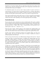
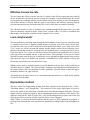
Each stage could represent an increase of a magnitude or so in expenditure and a halving of the
uncertainty in the project cost-estimate. This process is illustrated, for hydro projects, in the
Accuracy of Project Cost Estimates figure [Gordon, 1989].
At the completion of each step, a "go or no go" decision is usually made by the project proponent
as to whether to proceed to the next step of the development process. High quality, but low-cost,
pre-feasibility and feasibility studies are critical to helping the project proponent "screen out"
projects that do not make financial sense, as well as to help focus development and engineering
efforts prior to construction. The RETScreen Clean Energy Project Analysis Software can be
used to prepare both the initial pre-feasibility analysis and the more detailed feasibility analysis.
BIOH.37
RETScreen® Software Online User Manual
Accuracy of Project Cost Estimates [Gordon, 1989]
Currency
To perform a RETScreen project analysis, the user may select a currency of their choice from the
"Currency" cell in the Cost Analysis worksheet.
The user selects the currency in which the monetary data of the project will be reported. For
example, if the user selects "$," all monetary related items are expressed in $.
Selecting "User-defined" allows the user to specify the currency manually by entering a name or
symbol in the additional input cell that appears adjacent to the currency switch cell. The currency
may be expressed using a maximum of three characters ($US, £, ¥, etc.). To facilitate the
presentation of monetary data, this selection may also be used to reduce the monetary data by a
factor (e.g. $ reduced by a factor of a thousand, hence k$ 1,000 instead of $ 1,000,000).
If "None" is selected, all monetary data are expressed without units. Hence, where monetary data
is used together with other units (e.g. $/kWh) the currency code is replaced with a hyphen
(-/kWh).
The user may also select a country to obtain the International Standard Organisation (ISO) threeletter country currency code. For example, if Afghanistan is selected from the currency switch
BIOH.38
RETScreen® Biomass Heating Project Model
drop-down list, all project monetary data are expressed in AFA. The first two letters of the
country currency code refer to the name of the country (AF for Afghanistan), and the third letter
to the name of the currency (A for Afghani).
For information purposes, the user may want to assign a portion of a project cost item in a
second currency, to account for those costs that must be paid for in a currency other than the
currency in which the project costs are reported. To assign a cost item in a second currency, the
user must select the option "Second currency" from the "Cost references" drop-down list cell.
Some currency symbols may be unclear on the screen (e.g. €); this is caused by the zoom settings
of the sheet. The user can then increase the zoom to see those symbols correctly. Usually,
symbols will be fully visible on printing even if not fully appearing on the screen display.
Cost references
The user selects the reference (from the Cost Analysis worksheet) that will be used as a guideline
for the estimation of costs associated with the implementation of the project. This feature allows
the user to change the "Quantity Range" and the "Unit Cost Range" columns. The options from
the drop-down list are: "Canada - 2000," "None," "Second currency" and a selection of 8 userdefined options ("Enter new 1," "Enter new 2," etc.).
If the user selects "Canada - 2000" the range of values reported in the "Quantity Range" and
"Unit Cost Range" columns are for a 2000 baseline year, for projects in Canada and in Canadian
dollars. This is the default selection used in the built-in example in the original RETScreen file.
Selecting "None" hides the information presented in the "Quantity Range" and "Unit Cost
Range" columns. The user may choose this option, for example, to minimise the amount of
information printed in the final report.
If the user selects "Second currency" two additional input cells appear in the next row: "Second
currency" and "Rate: 1st currency/2nd currency." In addition, the "Quantity Range" and "Unit
Cost Range" columns change to "% Foreign" and "Foreign Amount," respectively. This option
allows the user to assign a portion of a project cost item in a second currency, to account for
those costs that must be paid for in a currency other than the currency in which the project costs
are reported. Note that this selection is for reference purposes only, and does not affect the
calculations made in other worksheets.
If "Enter new 1" (or any of the other 8 selections) is selected, the user may manually enter
quantity and cost information that is specific to the region in which the project is located and/or
for a different cost base year. This selection thus allows the user to customise the information in
the "Quantity Range" and "Unit Cost Range" columns. The user can also overwrite "Enter new
1" to enter a specific name (e.g. Japan - 2001) for a new set of unit cost and quantity ranges. The
user may also evaluate a single project using different quantity and cost ranges; selecting a new
range reference ("Enter new 1" to "Enter new 8") enables the user to keep track of different cost
scenarios. Hence the user may retain a record of up to 8 different quantity and cost ranges that
can be used in future RETScreen analyses and thus create a localised cost database.
BIOH.39
RETScreen® Software Online User Manual
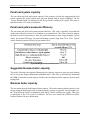
Second currency
The user selects the second currency; this is the currency in which a portion of a project cost item
will be paid for in the second currency specified by the user. The second currency option is
activated by selecting "Second currency" in the "Cost references" drop-down list cell. This
second unit of currency is displayed in the "Foreign Amount" column.
If the user selects "$," the unit of currency shown in the "Foreign Amount" column is "$."
Selecting "User-defined" allows the user to specify the currency manually by entering a name or
symbol in the additional input cell that appears adjacent to the currency switch cell. The currency
may be expressed using a maximum of three characters ($US, £, ¥, etc.). To facilitate the
presentation of monetary data, this selection may also be used to reduce the monetary data by a
factor (e.g. $ reduced by a factor of a thousand, hence k$ 1,000 instead of $ 1,000,000).
If "None" is selected, no unit of currency is shown in the "Foreign Amount" column.
The user may also select a country to obtain the International Standard Organisation (ISO) threeletter country currency code. For example, if Afghanistan is selected from the currency switch
drop-down list, the unit of currency shown in the "Foreign Amount" column is "AFA." The first
two letters of the country currency code refer to the name of the country (AF for Afghanistan),
and the third letter to the name of the currency (A for Afghani).
Some currency symbols may be unclear on the screen (e.g. €); this is caused by the zoom settings
of the sheet. The user can then increase the zoom to see those symbols correctly. Usually,
symbols will be fully visible on printing even if not fully appearing on the screen display.
Rate: 1st currency/2nd currency
The user enters the exchange rate between the currency selected in "Currency" and the currency
selected in "Second currency." The exchange rate is used to calculate the values in the "Foreign
Amount" column. Note that this selection is for reference purposes only, and does not affect the
calculations made in other worksheets.
For example, the user selects the Afghanistan currency (AFA) as the currency in which the
monetary data of the project is reported (i.e. selection made in "Currency" input cell) - this is the
1st currency. The user then selects United States currency (USD) from the "Second currency"
input cell - this is the 2nd currency. The user then enters the exchange rate in the "Rate:
AFA/USD" input cell i.e. the amount of AFA needed to purchase 1 USD. Using this feature the
user can then specify what portion (in the "% Foreign" column) of a project cost item's costs will
be paid for in USD.
BIOH.40
RETScreen® Biomass Heating Project Model
% Foreign
The user enters the percentage of an item's costs that will be paid for in the second currency. The
second currency is selected by the user in the "Second currency switch."
Foreign Amount
The model calculates the amount of an item's costs that will be paid for in the second currency.
This value is based on the exchange rate and the percentage of an items costs that will be paid for
in the second currency, as specified by the user.
Initial Costs (Credits)
The initial costs associated with the implementation of a biomass and/or WHR heating project
are detailed below. The major categories include costs for preparing a feasibility study,
performing the project development functions, completing the necessary engineering, purchasing
and installing the energy equipment, construction of the balance of plant and costs for any other
miscellaneous items.
Feasibility Study
Once a potential cost-effective biomass and/or WHR heating project has been identified through
the RETScreen pre-feasibility analysis process, a more detailed feasibility analysis study may be
required. This is particularly the case for large projects, with more than one building. Feasibility
studies typically include such items as a site investigation, a local biomass resource assessment, a
preliminary project design, and a final report. Feasibility study project management and travel
costs are also normally incurred. These costs are detailed in the following section.
For small projects (single buildings with small heating requirement), the cost of the feasibility
study, relative to the cost of the biomass and/or WHR heating system, may not be justified. In
this case the project proponent may choose to go directly to the engineering stage (combining
some steps from the feasibility and development stages).
Note: The RETScreen Clean Energy Project Analysis Software can also be used to prepare the
Feasibility Study.
Site investigation
A site investigation is normally required for biomass and/or WHR heating projects with district
heating. The site visit involves a brief survey of all major buildings under consideration. In small
district heating systems, the user would likely look for clusters of oil or electricity heated
buildings with a distance not exceeding 500 m. Typical major buildings heated with oil or
electricity include schools, hospital/health clinics, churches, senior's apartments, service garages
and community offices.
BIOH.41
RETScreen® Software Online User Manual
The identification of the most promising buildings or clusters is generally followed by a detailed
site and building or clusters analysis. The analysis includes: measurement of the distance
between the various buildings; determination of the fuel consumption for each building;
measurement of the building areas and insulation levels; study and documentation of the existing
building heating systems and locations, including notes on any attributes or problems for
conversion to biomass energy; selection of a possible site for the biomass heating plant;
preparation of a layout of approach roads and a plant yard for outdoor storage of chipped wood.
Site visit time includes the time required to arrange meetings, survey the site, obtain the
necessary information and any travel time (but not travel expenses - see "Travel and
accommodation".)
The time required for a site survey, detailed building and site analysis varies according to the
number of buildings involved and the complexity of the existing heating system. Obtaining fuel
consumption data can sometimes add to the time required. The cost of a site visit is influenced by
the planned duration and travel time to and from the site. The range at the site is typically 7 to
16 hours at a rate of approximately $40/h to $100/h.
Biomass resource assessment
Biomass and/or WHR heating projects are not considered "renewable energy" unless the biomass
is harvested in a sustainable manner. The user must carefully consider the biomass resource to
ensure that there is a sufficient local biomass resource to meet the projects energy requirements
in a environmentally appropriate and financially feasible manner. With small-commercial wood
biomass systems, it is unlikely that the annual woodchip consumption will exceed 1,500 tonnes,
which is relatively small for most forested regions. Because of this limited wood resource use, it
is assumed here that only a brief biomass resource assessment is required during the feasibility
analysis stage.
One basic question must be answered by the user: "Are there substantial sustainable wood
resources within a reasonable transport distance using efficient vehicles?" This can be addressed
by conducting a brief aerial survey or by travelling surrounding roads and waterways to assess
standing wood resources.
The time required to carry out a brief biomass resource assessment is typically 6 to 12 hours,
depending on the extent of the field survey and the amount of data collection and analysis
involved. Typical rates for biomass resource assessment experts range from $40/h to $100/h.
This assessment can usually be combined with the site investigation. The costs of charter flights
may need to be added if an aerial survey is required (add to "Travel and accommodation").
Preliminary design
A preliminary design that synthesizes the above information is required. The design is usually
based on design approaches used in most existing small biomass and/or WHR heating systems.
Some elements such as the building yard or approach roads will be specific to the proposed plant
sites.
BIOH.42
RETScreen® Biomass Heating Project Model
The time required for a preliminary design analysis is 6 to 8 hours, depending on the number of
buildings involved and any features unique to the site. The rate is approximately $40/h to $100/h.
Report preparation
A summary report should be prepared which describes the feasibility study, its findings and
recommendations. The written report will contain data summaries, charts, tables and illustrations
which clearly describe the proposed project. This report should be in sufficient detail regarding
costs, performance and risks to enable project lenders and other decision-makers to evaluate the
merits of the project.
The cost of the report preparation is calculated based on an estimate of the time required by a
professional to complete the necessary work, and should also include the time required to
manage the overall feasibility study preparation. Typically 16 to 32 hours is required. The major
variables are: the number of buildings involved; the complexity of interconnecting the buildings;
any unique requirements regarding the location of the plant, any unusual wood supply
requirements (e.g. the need for a wood supply yard), and conclusions and recommendations
regarding the supply of woodchips. The rate is approximately $40/h to $100/h.
Travel and accommodation
This cost item includes all travel related costs (excluding time) required to prepare all sections of
the feasibility study by the various members of the feasibility study team. These expenses
include such things as airfare, car rental, lodging and per diem rates for each trip required. For
local travel, a supplier may not charge for time and expenses. For isolated areas, where air travel
is time consuming and expensive, it may be better to include more than one potential project in
the feasibility study to spread the site visit costs over a number of projects and not just one
building.
In the case of isolated areas, rates for air travel will vary considerably. Airfares are typically
twice those for similar distances in populated areas. Since travel is a large component of the cost
of doing work in isolated areas and the range of cost so variable it is advised to contact a travel
agent with experience in arranging such travel. Accommodation rates are typically twice the
going rate for modest accommodation in populated areas. Typical rates for modest hotel rooms
can range from $180 to $250 per day in the more isolated areas.
Other
These input cells are provided to allow the user to enter cost or credit items that are not included
in the information provided in the above cost category. The user must enter a positive numerical
value in the "Unit Cost" column.
A cost item may be entered in the grey input cell as "Other." The user then selects "Cost" from
the drop-down list in the unit column. The user can input both a quantity amount and unit cost.
BIOH.43
RETScreen® Software Online User Manual
This item is provided to allow for project, technology and/or regional differences not specifically
covered in the generic information provided.
A credit item may be entered in the grey input cell as "Credit." The user then selects "Credit"
from the drop-down list in the unit column. The project may be credited for material and/or
labour costs that would have been spent on the base case, or conventional, energy system. The
user can input both a quantity amount and unit cost. Note that the credit item is expressed as a
negative value in the "Amount" column.
Development
Once a potential biomass and/or WHR heating project has been identified through the feasibility
study to be desirable to implement, project development activities may follow. For some
projects, the feasibility study, development and engineering activities may proceed in parallel,
depending on the risk and return acceptable to the project proponent.
For biomass heating projects with district heating, there are a number of possible project
developers. Currently, a common approach is for the client to be the building owner with the
developer being the local biomass and/or WHR system product supplier who provides complete
design/build services. General contractors may also be the developer, purchasing the biomass
and/or WHR heating system on behalf of the building owner. It is also possible that an Energy
Services Company (ESCO) or the local community utility or public works department could be
the project developer, where they purchase the biomass and/or WHR heating system and sell the
energy to local building owners. Estimating the costs of the development phase will depend on
the particular development arrangement established. Items here include costs for contract
negotiations, permits and approvals, project financing, development phase project management
and any development related travel costs. These costs are detailed in the following section.
Contract negotiations
If there is a decision to proceed with the project based on a positive result of the feasibility study,
the project proponent will need to establish a fiscal operating arrangement and negotiate a
contract with one or more appropriate project stakeholders.
This can be very time consuming, particularly if there are a number of different stakeholders
involved, for example, a fuel supplier, a heating plant operator and several clients who wish to
purchase heat. The time required typically ranges from 32 to 80 hours at rates ranging from
$50/h to $100/h.
Permits and approvals
A number of permits and approvals may be required by local authorities for the construction of
the project. The cost of acquiring the necessary permits and approvals is calculated based on an
estimate of the time required to complete the necessary work. These agencies include local
BIOH.44
RETScreen® Biomass Heating Project Model
building and electrical inspectors, boiler inspectors, fire safety inspectors, forestry (fuel supply)
and an emissions regulating authority.
The time required depends on the number of agencies involved and what is specifically required
to meet their rules and regulations. The time requirement is typically 40 to 80 hours at rates
ranging from $40/h to $100/h. The user can also add to the number of hours, or unit costs, an
amount to cover the actual permit itself. Permit costs are usually minor relative to the total
project cost.
Project financing
The time and effort required to arrange project financing will vary depending upon the project
developer and client relationship. In most cases, where the client is the building owner and the
developer is the product supplier, the project financing costs attributable to the project are
minimal. The building owner will usually finance the project out of capital or O&M budgets and
the product supplier will provide in-kind support as required to help arrange the client project
financing. In the case of an ESCO or local utility developed project much more effort will likely
be required to arrange financing, negotiate an energy services contract with the building owner
and prepare legal documents.
The cost to obtain project financing will range from 32 to 48 hours at a rate of between $50/h to
$100/h. The lower end of the range is for building owner/product supplier developed projects.
The higher end of the range applies to ESCO/utility type projects.
Project management
The project management cost item should cover the estimated expenses of managing all phases
of the development of the project (excluding construction supervision). Public relations are also
included here. The time required for public relations varies according to the technical complexity
of the project, the number of stakeholders involved, the volume of fuel required and the size of
the potential fuel supply area.
The elapsed time for the development of a biomass and/or WHR heating project falls in the mid
range as compared with other projects. Projects can be developed within a one to two year time
period. The project development management time will usually take between 30 to 80 hours at
rates of between $50/h to $100/h.
Travel and accommodation
This cost item includes all travel related costs (excluding time) required to develop the project.
BIOH.45
RETScreen® Software Online User Manual
Other
These input cells are provided to allow the user to enter cost or credit items that are not included
in the information provided in the above cost category. The user must enter a positive numerical
value in the "Unit Cost" column.
A cost item may be entered in the grey input cell as "Other." The user then selects "Cost" from
the drop-down list in the unit column. The user can input both a quantity amount and unit cost.
This item is provided to allow for project, technology and/or regional differences not specifically
covered in the generic information provided.
A credit item may be entered in the grey input cell as "Credit." The user then selects "Credit"
from the drop-down list in the unit column. The project may be credited for material and/or
labour costs that would have been spent on the base case, or conventional, energy system. The
user can input both a quantity amount and unit cost. Note that the credit item is expressed as a
negative value in the "Amount" column.
Engineering
The engineering phase includes costs for the biomass and/or WHR heating plant site and
building design, energy system design, tenders and contracting, and construction supervision. If
the project is awarded on a design/build basis, then all of these costs would be included in prices
provided by the equipment supplier or contractor responsible for the project. If the project is
awarded by tender based on specifications prepared by a consultant, then there will be
engineering charges from the consultant overseeing the project and perhaps the equipment
supplier.
Site and building design
Site layout includes the selection of the building or cluster of buildings to be heated by the
biomass and/or WHR heating system; selecting the site for the biomass heating plant;
determining where approach roads should go for site access and determining the boundaries of
the plant yard. The buildings used to house small-commercial heating plants and for fuel storage
are usually similar to a heated garage. The buildings must have a concrete floor and the walls of
the fuel storage reserve must be strong enough to permit the use of a front end loader.
The time required to carry out a site layout and building design is typically 12 to 18 hours.
Variables include site restrictions, type of delivery vehicles to be used and the turning space
required and space needed to store woodchips. Rates of $40/h to $100/h are common.
Energy system design
The heating plant design is generally quite straight forward for small-commercial biomass
systems with only small variations. Factors to be determined include: the number of
burner/boiler units; the size/capacity of the units; the fuel type; the auger size; the auger speed;
BIOH.46
RETScreen® Biomass Heating Project Model
the gearbox reduction ratio; the auger motor size (3/4 or 1 hp); and unique system options such
as alarms. The heat distribution system design is an important design component in smallcommercial biomass systems. Design tasks include: selection of a routing for the heat
distribution piping; determining the appropriate diameter of piping; determining where and how
to interconnect with the heating systems of the various buildings; and selecting and locating any
heat metres to be used.
The time required to design a biomass and/or WHR heating system is typically 14 to 30 hours at
rates of $40/h to $100/h. The primary time variables are: the level of automation required; the
number of buildings involved; the different types of heat distribution systems present in the
existing buildings (e.g. hot water, hot air); and the ease or difficulty of interconnecting with each
building.
Tenders and contracting
Upon completion of the various engineering tasks, tender documents may be required by the
project developer. They are prepared for the purpose of selecting contractors to undertake the
work. Once tenders are released, the contracting process is required to both negotiate and
establish contracts for the completion of the project.
The time required to produce a set of bid documents will vary depending upon the complexity
and the size of the project. If bid documents are required 12 to 20 hours at rates of $40/h to
$100/h are possible.
Construction supervision
The construction supervision cost item summarises the estimated costs associated with ensuring
that the project is constructed as designed. Construction supervision is provided either by the
consultant overseeing the project or by the equipment supplier, or the project manager.
Construction supervision involves regular visits to the job site to inspect the installation.
Depending of the project size, this task can take between 30 to 80 hours at rates of $40/h to
$100/h. Travel time to the site for construction supervision is in addition to the range given.
Travels costs should be included in the "Development" section.
Other
These input cells are provided to allow the user to enter cost or credit items that are not included
in the information provided in the above cost category. The user must enter a positive numerical
value in the "Unit Cost" column.
A cost item may be entered in the grey input cell as "Other." The user then selects "Cost" from
the drop-down list in the unit column. The user can input both a quantity amount and unit cost.
This item is provided to allow for project, technology and/or regional differences not specifically
covered in the generic information provided.
BIOH.47
RETScreen® Software Online User Manual
A credit item may be entered in the grey input cell as "Credit." The user then selects "Credit"
from the drop-down list in the unit column. The project may be credited for material and/or
labour costs that would have been spent on the base case, or conventional, energy system. The
user can input both a quantity amount and unit cost. Note that the credit item is expressed as a
negative value in the "Amount" column.
Energy Equipment
The energy equipment, as defined here, includes the waste heat recovery system, biomass boilers
and burners, and the associated spare parts, chimney stacks, plumbing, electrical, equipment
installation and transportation costs. The user may refer to the RETScreen Online Product
Database for supplier contact information in order to obtain prices or other information required.
These costs are detailed below.
Waste heat recovery system
The user enters the waste heat recovery cost per kW. The kW capacity is transferred from the
Energy Model worksheet. This value includes both equipment and installation costs.
The cost for the waste heat recovery (WHR) system varies considerably depending on the source
of waste heat. For example, a reciprocating engine, with a 100 kW WHR system consisting of
heat exchangers, a control system for jacket cooling and a recovery boiler for exhaust gas and
lubrication oil, the typical cost would be $100,000 or $1,000/kW.
Biomass heating system
The user enters the biomass heating system cost per kW. The kW capacity (and number of
boilers) is transferred from the Energy Model worksheet. The following tables provide typical
values of "cost per capacity" in $/kW. The user may refer to the RETScreen Online Product
Database for supplier contact information in order to obtain prices or other information required.
The biomass boiler(s) cost is determined by the capacity. The price differential between the
biomass systems in each category is relatively small because the labour and many ancillary
components such as pumps, fittings and controls remain largely the same regardless of capacity.
The cost of biomass burner(s) is determined by the overall capacity and cost of components used.
However, the price differential between small burners and large ones is normally small. This is
due to the fact that certain standard components are required regardless of the capacity rating.
Examples include: the control panel; the auger drive motor; fabrication labour. Components for
which the costs vary somewhat include: reduction gearboxes; augers; size and weight of the fuel
hoppers and combustion cells.
BIOH.48
RETScreen® Biomass Heating Project Model
Typical range of costs for small-commercial biomass systems are illustrated in the following
table:
Small-Commercial Biomass System Costs
The user should refer to the biomass boiler system capacity to select the appropriate cost for the
burner. The number of biomass burners is assumed (for this level of analysis) to be equal to the
number of biomass boilers. The burners normally range from 1 to 3 units.
Typical range of costs for commercial/industrial biomass systems are illustrated in the following
table:
Commercial/Industrial Biomass System Costs
The biomass systems given in the previous table are built for commercial or industrial usage and
are more heavy duty than small-commercial biomass systems. The above costs include automatic
fuel handling system, combustion chamber, boiler, fluegas handling equipment, induced draft
fan, multi-cyclone or wet venturi scrubber, stack and 1% for initial spare parts.
For systems with district heating, the cost of the distribution pump and the cost of installation are
included in the pipe costs. The size and cost of the pumps (typically one for operations and one
for standby or emergency) vary by the size and complexity of the system. The built-in formulas
for estimating pipe costs include the cost of the pump and the cost of installation.
Biomass equipment installation
The user enters the biomass equipment installation costs per kW. The kW capacity of the
biomass heating system is transferred from the Energy Model worksheet.
Typical equipment installation costs for small-commercial and commercial/industrial boilers are
illustrated in the following tables.
BIOH.49
RETScreen® Software Online User Manual
Small-Commercial Boiler Installation Costs
Commercial/Industrial Boiler Installation Costs
Installation costs for district heating distribution pumps are included in the pipe costs.
Transportation
The transportation costs for the biomass heating and/or WHR system equipment vary depending
on weight and size of material to be shipped and distance from the factory. Normally, the
material is shipped by truck unless there is no road access to the site, in which case, other
methods, such as rail, air, winter road or boat are required. Some projects will require more than
one freight carrier. For example, truck to rail line, then to a barge or plane. Each time the
material is transferred, someone must be on hand to receive it and/or arrange for the transfer.
Freight costs to isolated areas may be difficult to estimate and it is advisable to check for best
routing.
As an example, the weight of the energy equipment for a common biomass heating system sold
in North America is approximately 460 kg for a 75 kW unit (biomass burner, boiler and
miscellaneous parts) and 1,840 kg for a 200 kW unit.
Other
These input cells are provided to allow the user to enter cost or credit items that are not included
in the information provided in the above cost category. The user must enter a positive numerical
value in the "Unit Cost" column.
A cost item may be entered in the grey input cell as "Other." The user then selects "Cost" from
the drop-down list in the unit column. The user can input both a quantity amount and unit cost.
BIOH.50
RETScreen® Biomass Heating Project Model
This item is provided to allow for project, technology and/or regional differences not specifically
covered in the generic information provided.
A credit item may be entered in the grey input cell as "Credit." The user then selects "Credit"
from the drop-down list in the unit column. The project may be credited for material and/or
labour costs that would have been spent on the base case, or conventional, energy system. The
user can input both a quantity amount and unit cost. Note that the credit item is expressed as a
negative value in the "Amount" column.
Balance of Plant
The balance of plant for a biomass and/or WHR heating project typically includes a number of
items such as a peak load heating system, and possibly a back-up heating system. It will also
include the heat distribution system components such as distribution piping and trenching, and
the balance of plant will include the building interconnection plumbing required. In addition,
plant building and yard will usually have to be constructed and separate costs for equipment
installation and transportation will be included. These costs are detailed below. The user should
remember to consider cost items, listed below, that may be "credited" due to the fact that they
are required even if the biomass and/or WHR heating project does not go forward. The user
should try to establish the capital cost of equipment that would be installed as an alternative to
the biomass and/or WHR heating system. Typically, there are four alternatives, in order of
largest to lowest potential capital cost crediting:
1. New construction where a district heating system is considered "conventional."
2. New construction where a district heating system would not otherwise be planned.
3. Retrofit situations when there are plans to either repair or upgrade an existing heating
system.
4. Retrofit situations when there are no plans to either repair or upgrade an existing
heating system.
[Biomass] Peak load heating system
As discussed in the Energy Model description, a typical biomass and/or WHR heating system
includes a heating system that is utilised to meet the peak period load.
The cost of a peak load heating system ranges from approximately $85/kW for large oil units
(e.g. 400 kW unit), to $100/kW for small oil units (e.g. 75 kW unit). The cost of an oil tank,
plumbing and breaching (smoke pipe) should also be included, these costs range from $3,000 to
$6,000 for each boiler. The capacity of the boiler(s) is automatically copied from the Energy
Model worksheet. The combined costs will likely range from approximately $10,000 to $34,000
($133/kW to $85/kW) per oil boiler.
BIOH.51
RETScreen® Software Online User Manual
Back-up heating system
As discussed in the Energy Model section, a typical biomass and/or WHR heating system may
also include an optional back-up heating system which will provide back-up in case of a heating
system shut-down. The installation of a new oil- fired back-up heating system may be necessary
unless the existing boiler can be utilised as a back-up.
The cost of a back-up heating system ranges from $6,000 to $28,000 for oil boilers ranging in
size from 75 to 400 kW. The cost of plumbing and breaching (smoke pipe) should also be
included, these costs range from $3,000 to $4,000. The combined costs range from $9,000 to
$32,000 ($107/kW to $75/kW) per oil boiler (also see description of "Peak load heating system"
- note that the fuel tank is not included with the back-up heating system).
Energy transfer station(s)
The number of buildings and cost of the energy transfer station(s) is automatically copied from
the Heating Load & Network worksheet.
Secondary distribution line pipe
The total length and cost of the secondary distribution line pipe is automatically copied from the
Heating Load & Network worksheet.
Main distribution line pipe
The total length and cost of the main distribution line pipe is automatically copied from the
Heating Load & Network worksheet.
Building and yard construction
To prepare an initial estimate of the total building and yard construction cost, the user could
simply insert the building size and then use a combined cost based on plant building of $220/m²
to $470/m².
Typical building sizes for small-commercial biomass combustion systems are given in the table.
Typical Building Sizes for Small-Commercial Biomass Systems
BIOH.52
RETScreen® Biomass Heating Project Model
Note that for a 2,500 kW system, fuel storage space should also be included. The building,
including the fuel reserve space, should be insulated to keep the woodchips from freezing. Free
space may be used as a heated work space. The buildings will have a concrete pad with
containment walls at the front door upon which vehicles can dump fuel, unless a small enough
vehicle is available to unload inside the building.
Plant building construction material costs will likely range from $170/m² to $350/m². The user
should obtain an estimate from local building contractors as this item can represent a significant
amount of the total project costs. Other uses for the building (e.g. workshop, lumber drying kiln,
etc.) should also be considered. Existing buildings should be used if possible to help avoid this
cost.
The length of approach roads and the area of the yard vary, depending on the particular site, the
volume of wood that is to be stored in the yard and the delivery vehicles that are to be used. The
roads and yards must permit vehicles to manoeuvre and back up without difficulty. Making them
too small could cause a lot of problems.
The cost of approach roads and yard construction vary significantly, depending on the required
road and yard area, the soil material and the proximity of gravel pits. The cost is typically
$100/m² to $200/m² and sizes range between 90 to 150 m². In some cases additional land may
need to be purchased for the yard and building construction. If this is the case, add the land costs
in $/m², to the yard construction costs. If land is to be leased, include the lease cost under
"Other" in the "Annual Costs" section.
Equipment installation
The labour required to install the balance of plant will typically range from $25/h to $50/h and
will require 500 to 700 hours to construct the building, and carry out the installation of all the
equipment listed above for the "Balance of Plant" sub-section.
Transportation
The transportation costs for the biomass system equipment vary depending on weight and size of
material to be shipped and distance from the factory. Normally, the material is shipped by truck
unless there is no road access to the site, in which case, other methods, such as rail, air, winter
road or boat are required. Some projects will require more than one freight carrier. For example,
truck to rail line, then to a barge or plane. Each time the material is transferred, someone must be
on hand to receive it and/or arrange for the transfer. Freight costs to isolated areas may be
difficult to estimate and it is advisable to check for best routing.
As an example, a 75 kW oil boiler weighs approximately 770 kg while a 400 kW oil boiler
weighs approximately 5,900 kg.
BIOH.53
RETScreen® Software Online User Manual
Other
These input cells are provided to allow the user to enter cost or credit items that are not included
in the information provided in the above cost category. The user must enter a positive numerical
value in the "Unit Cost" column.
A cost item may be entered in the grey input cell as "Other." The user then selects "Cost" from
the drop-down list in the unit column. The user can input both a quantity amount and unit cost.
This item is provided to allow for project, technology and/or regional differences not specifically
covered in the generic information provided.
A credit item may be entered in the grey input cell as "Credit." The user then selects "Credit"
from the drop-down list in the unit column. The project may be credited for material and/or
labour costs that would have been spent on the base case, or conventional, energy system. The
user can input both a quantity amount and unit cost. Note that the credit item is expressed as a
negative value in the "Amount" column.
Miscellaneous
This category is for all of the miscellaneous costs that occur during a project and have not been
taken into account in the previous sections. For biomass and/or WHR heating projects these costs
can include, contractors overhead, training and contingencies.
Overhead
A general contractor will normally apply a mark-up on their costs to cover overhead and on subcontractors costs to cover contract administration. The overhead rate ranges from 10 to 30% of
the entire project cost. For biomass and/or WHR heating projects, another way to estimate this
cost is to consider the time a general contractor, or project manager would be required to manage
the construction of the project. A range of 36 to 120 hours, depending upon the scale of the
project, at rates of $50/h to $100/h could be expected. The incremental overhead includes only
the amount directly related to the energy project. Any overhead that would otherwise be
allocated to the "conventional" energy system should not be included here.
Training
The training required by automated biomass plant operators varies, depending on their
responsibilities and capabilities. The training ranges from about 8 hours for basic operation
training to about 30 hours for skilled operators who are being trained to handle all aspects of
operation and repairs. Repairs mainly involve replacement of electrical components such as
motors, capacitors, timers, contractor switches, aquastats as well as mechanical components such
as the fuel agitator and the feed auger. The training rate is approximately $40/h to $100/h.
BIOH.54
RETScreen® Biomass Heating Project Model
Contingencies
The allowance made for contingency costs depends on the level of accuracy of the cost
estimates. Contingencies are estimated based on a user-selected percentage of the sub-total of all
project costs. Note that contingencies are incremental in the sense that they are derived from
project costs including any credits.
The allowance for contingency items should be based on the level of accuracy associated with
the RETScreen pre-feasibility estimate of the project costs. Typically, a pre-feasibility level cost
analysis should be accurate within 40 to 50%. However, this accuracy will depend on the
expertise of the study team, the scale of the project being considered, the level of effort put
forward to complete the pre-feasibility study and the availability of accurate information. It is
certainly possible that the RETScreen user experienced with biomass and/or WHR heating
project developments could estimate costs in the range of 5 to 40% of the total initial project
costs.
Annual Costs (Credits)
There are a number of annual costs associated with the operation of a biomass and/or WHR
heating system. These could include property taxes, insurance, spare parts, O&M labour, travel
and accommodations and general, administrative expenses and contigencies. In addition, costs
for biomass fuel, peak load fuel oil and parasitic electricity consumption will also be incurred.
These costs are detailed in the following section.
O&M
Property taxes/Insurance
Generally, biomass and/or WHR heating systems should not increase property taxes, with the
exception of the plant building constructed. In some cases, a community may even provide a tax
incentive for biomass and/or WHR heating installations. The owners of a biomass and/or WHR
heating system will normally require insurance to protect their interests. This will include: fire
insurance, public liability insurance and accident insurance to cover repairs in the event of
accidental damage.
The cost of fire insurance; public liability insurance and accident insurance normally amount to
$500 to $1,500 per year. The costs vary, depending on the capital value of the biomass and/or
WHR heating system and whether the heating plant must be insured on its own or whether
insurance for the plant is merely added to insurance for other equipment and facilities. A more
accurate cost can be estimated by contacting an insurance broker.
Spare parts
The annual maintenance and repair costs for "wear items" in small-commercial biomass plants
range from roughly $200 to $600 per year per burner. For larger systems use 1% of equipment
BIOH.55
RETScreen® Software Online User Manual
costs. The variables include: the number of burners; the size of the fuel hopper and the fuel type.
Larger fuel hoppers have greater mechanical stresses. Sawdust and bark generally contain some
dirt that causes much more wear on fuel feed augers.
O&M labour
Labour is required to fill the fuel hopper and scraping the ash off the grate on a daily basis. Every
three to four weeks accumulated fly ash must be cleaned out of the boiler. Automated biomass
plants are rugged and reliable, but annual maintenance and repair labour costs must be expected
for "wear items" such as pumps, feed motors, capacitors and feed augers.
The labour for the filling of the fuel hopper, the scraping of the grate and for periodic cleaning of
the boiler normally takes 8 to 12 hours per month (96 to 144 hours per year) at a rate of $15/h to
$30/h. In many cases, the operator(s) perform these tasks as part of a job that includes other
related or non-related tasks.
For larger plants assume 1 to 2 hours per day for general maintenance including filling fuel
storage, monitoring of the equipment and emptying ash bins.
Travel and accommodation
For larger biomass and/or WHR heating systems in isolated areas, it is possible that an annual
allowance may be required for travel, room and board costs associated with annual maintenance
and inspection by an system expert. However, for well-designed and maintained systems this
will not be required.
General and administrative
Annual general and administrative costs include the costs of bookkeeping, preparation of annual
statements, bank charges, communication, a billing heat clients, etc. General and administrative
costs are project specific and depend on the nature of the business enterprise. These costs
normally start at a range of $500 to $2,000 per year and can be significantly higher for larger
scale projects with many heat clients.
Other
These input cells are provided to allow the user to enter cost or credit items that are not included
in the information provided in the above cost category. The user must enter a positive numerical
value in the "Unit Cost" column.
A cost item may be entered in the grey input cell as "Other." The user then selects "Cost" from
the drop-down list in the unit column. The user can input both a quantity amount and unit cost.
This item is provided to allow for project, technology and/or regional differences not specifically
covered in the generic information provided.
BIOH.56
RETScreen® Biomass Heating Project Model
A credit item may be entered in the grey input cell as "Credit." The user then selects "Credit"
from the drop-down list in the unit column. The project may be credited for material and/or
labour costs that would have been spent on the base case, or conventional, energy system. The
user can input both a quantity amount and unit cost. Note that the credit item is expressed as a
negative value in the "Amount" column.
Contingencies
A contingency allowance should be included to account for unforeseen annual expenses and will
depend on the level of accuracy of the operation and maintenance cost estimate section. It is
usual to carry a contingency allowance for at least the replacement of the most expensive
component subject to catastrophic failure. The contingency allowance is calculated based on an
estimated percentage of the other operation and maintenance costs. It typically ranges from 1.25
to 10%, but could be as high as 20%. This is especially true in the case of project in isolated
areas. To meet repair costs for a biomass and/or WHR heating system a contingency fund of
$2,000 to $3,000, depending on the size and fuel type, is minimally required.
Fuel/Electricity
Waste heat
The Energy Model worksheet calculates the amount of waste heat used on an annual basis. This
value is copied to the Cost Analysis worksheet.
The user enters the cost of waste heat in $/MWh. A cost might be charged if the owner of the
waste heat is not the developer of the biomass and/or WHR heating system. In other cases
removing the waste heat can improve the generators efficiency and no cost or a negative cost is
applied.
Biomass
The Energy Model worksheet calculates the amount of biomass fuel used on an annual basis.
This value is copied to the Cost Analysis worksheet.
Biomass fuel (e.g. woodchips or sawdust) may be purchased from a separate independent
company on a weight or volume basis. Alternatively, the organisation that owns and operates the
biomass heating plant may also have a forest operation and produce its own fuel. However, for
the purpose of this analysis, methods for supplying biomass fuel are not covered in detail. At the
pre-feasibility analysis stage, a range of values for biomass fuel, in $/tonne, is sufficient to
prepare a study. The user can perform a sensitivity analysis for various biomass fuel costs. If the
biomass and/or WHR heating project passes this "quick screen" during the pre-feasibility
analysis study, the follow-up feasibility level analysis can consider various supply options in
much more detail.
BIOH.57
RETScreen® Software Online User Manual
Typical costs for biomass fuel (e.g. woodchips or sawdust) range from $0/tonne to $85/tonne. In
some cases wood waste may be available at no charge ($0) to the biomass plant owner other than
loading and trucking costs. For example, retail prices (delivered to large customers) for
woodchips in the area of Charlottetown, Prince Edward Island are in the range of $27/tonne. The
retail price of sawmill waste is in the range of $15/tonne [McCallum, 1995]. In isolated areas,
biomass fuel costs can be significantly higher (as high as $85/tonne). The user may want to
contact the local government forestry office or local woodchip suppliers to obtain more
information on local fuel woodchip costs.
Peak load system fuel
The Energy Model worksheet calculates the volume of peak load heating system fuel required on
an annual basis. This value is copied to the Cost Analysis worksheet.
Cost for peak load heating system fuel in a specific location can be obtained from local suppliers.
The purchase of fuel for peak load heating purposes is usually under the responsibility of the
heating plant owner assuming that the boiler is located in the biomass heating plant. In some
cases, the peak load heating systems may be located in the client buildings and the client may
then incur the charges for the peak load system fuel.
Parasitic electricity
The parasitic electricity is the electrical energy required to run the biomass and/or WHR heating
system, and the district heating distribution pumps on an annual basis. The user enters the
approximate kWh electrical consumption in the quantity cell and the price of electricity ($/kWh)
in the unit cost cell.
A rough estimate of the parasitic electricity required to run the biomass and/or WHR heating
system is approximately 1 to 2% of the total annual energy delivered by the biomass system. The
low end is for larger systems while the higher end of the range is for smaller systems.
Small-commercial biomass systems use electricity to run the fuel feed system, the burner fan and
the circulation pumps. The electricity to run the fuel feed system, the burner fan and the
circulation pumps of a small commercial biomass system can vary from roughly 2,000 kWh for
small systems (75 kW) to 6,000 kWh for large systems (250 kW).
For a commercial size biomass system the parasitic load varies between manufacturers – The
following table can be used as a guideline.
Parasitic Load for Commercial Size Biomass Systems
BIOH.58
RETScreen® Biomass Heating Project Model
For a system with less than 500 m of total pipe length and 500 kW of peak heating load, the
parasitic electricity for the district heating distribution pumps can be estimated to be 0.5 kW. The
approximate district heating pump load for a larger district heating system can be estimated using
the following formula:
P
= M*Q*C/T
P
= pump load (kW)
where:
M = total pipe length for main distribution line (m)
Q = total peak heating load (kW)
C
= constant, 58.7*10^-6 (ºC/m)
T
= difference between the supply temperature and the return temperature of the
distribution system
The parasitic annual demand can be estimated using the following formula:
D
= P*E
D
= parasitic annual demand (kWh)
P
= pump load (kW)
E
= equivalent full load hours (h)
where:
For example, the pump capacity for a system with 2,000 m total pipe length, 1,500 peak heating
load and 40ºC differential temperature is estimated as follows:
P
= 2,000 m * 1,500 kW * 58.7*10^-6ºC/m /40ºC
= 4.4 kW
With 2,500 equivalent full load hours the parasitic annual demand for the distribution pumps is
estimated as follows:
D = 4.4 kW * 2,500 h
= 11,000 kWh
BIOH.59
RETScreen® Software Online User Manual
Periodic Costs (Credits)
This section is provided to allow the user to specify the periodic costs associated with the
operation of the system over the project life. Grey input cells are provided to allow the user to
enter the name of a periodic cost and periodic credit item. The user must enter a positive
numerical value in the "Unit Cost" column.
A periodic cost represents recurrent costs that must be incurred at regular intervals to maintain
the project in working condition. A periodic cost item is entered in the grey input cell. The user
then selects "Cost" from the drop-down list in the unit column. The interval (in years) over
which the periodic cost is incurred is entered in the period column. The amount of the cost
incurred at each interval is entered in the unit cost column.
The project may also be credited for periodic costs that would have been incurred over the
project life of the base case, or conventional, energy system. The periodic credit item is entered
in the grey input cell. The user then selects "Credit" from the drop-down list in the unit column.
The interval (in years) over which the periodic credit is incurred is entered in the period column.
The amount of the credit incurred at each interval is entered in the unit cost column. Note that
the credit item is expressed as a negative value in the "Amount" column.
End of project life
The user enters the value of the project at the end of its life. This amount is also commonly
referred to as the salvage value (or disposal value). If the salvage value of the project at the end
of its life is positive, then the user selects "Credit" from the drop-down list in the unit column in
order to express this item as a negative value. However, if the costs of remediation or
decommissioning that must be incurred at the end of the project life exceed the salvage value,
then the user must select "Cost" from the drop-down list. The user must enter a positive
numerical value in the "Unit Cost" column.
Note: At this point, the user should go to the optional GHG Analysis worksheet.
BIOH.60
RETScreen® Biomass Heating Project Model
Financial Summary
As part of the RETScreen Clean Energy Project Analysis Software, a Financial Summary
worksheet is provided for each project evaluated. This common financial analysis worksheet
contains six sections: Annual Energy Balance, Financial Parameters, Project Costs and
Savings, Financial Feasibility, Yearly Cash Flows and Cumulative Cash Flows Graph. The
Annual Energy Balance and the Project Costs and Savings sections provide a summary of the
Energy Model, Cost Analysis and GHG Analysis worksheets associated with each project
studied. In addition to this summary information, the Financial Feasibility section provides
financial indicators of the project analysed, based on the data entered by the user in the Financial
Parameters section. The Yearly Cash Flows section allows the user to visualise the stream of pretax, after-tax and cumulative cash flows over the project life. The Financial Summary worksheet
of each Workbook file has been developed with a common framework so the task of the user in
analysing the viability of different project types is made simpler. This also means the description
of each parameter is common for most of the items appearing in the worksheet.
One of the primary benefits of using the RETScreen software is that it facilitates the project
evaluation process for decision-makers. The Financial Summary worksheet, with its financial
parameters input items (e.g. discount rate, debt ratio, etc.), and its calculated financial feasibility
output items (e.g. IRR, simple payback, NPV etc.), allows the project decision-maker to consider
various financial parameters with relative ease. A description of these items, including comments
regarding their relevance to the preliminary feasibility analysis, is included below.
Annual Energy Balance
The summary items here are calculated and/or entered in the Energy Model and GHG Analysis
worksheets and transferred to the Financial Summary worksheet.
Project name
The user-defined project name is entered for reference purposes only in the Energy Model
worksheet, and it is copied automatically to the Financial Summary worksheet.
Project location
The user-defined project name is entered for reference purposes only in the Energy Model
worksheet, and it is copied automatically to the Financial Summary worksheet.
Renewable energy delivered
The Energy Model worksheet calculates the renewable energy delivered (MWh) by the project,
which is the sum of the waste heat recovery and biomass heating energy delivered.
BIOH.61
RETScreen® Software Online User Manual
Heating energy delivered
The Energy Model worksheet calculates the heating energy delivered (MWh). This energy
displaces the heating energy that would have otherwise been delivered by the base case heating
system. The heating energy delivered is used in conjunction with the weighted average avoided
cost of heating energy to calculate the heating energy savings.
Heating fuel displaced
The heating fuel displaced is the type of heating energy displaced by the addition of the project.
The heating fuel type selected for each cluster are entered in the Heating Load & Network
worksheet. The following types of fuels are available in the model: Natural gas, Propane, Diesel
(#2 oil), #6 oil, Electricity and Other.
Electricity required
The electricity required is the sum of the parasitic electricity entered in the Cost Analysis
worksheet and the electricity used by the peak load heating system, if any, as selected in the
Energy Model worksheet.
Net GHG emission reduction
The model calculates the net annual average GHG emission reduction in equivalent tonnes of
CO2 per year (tCO2/yr) resulting from the implementation of the system instead of the base case,
or baseline, heating system. This value is calculated in the GHG Analysis worksheet, and it is
copied automatically to the Financial Summary worksheet.
Net GHG emission reduction - credit duration
The model calculates the cumulative net greenhouse gas (GHG) emission reduction for the
duration of the GHG credit, in equivalent tonnes of CO2 (tCO2), resulting from the
implementation of the project instead of the base case, or baseline, system. This value is
calculated by multiplying the appropriate net annual GHG emission reduction by the GHG
reduction credit duration.
Net GHG emission reduction - project life
The model calculates the net project life GHG emission reduction for the duration of the project,
in equivalent tonnes of CO2 (tCO2) resulting from the installation of the project instead of the base
case, or baseline, heating system. This value is calculated by multiplying the net annual GHG
emission reduction by the project life.
BIOH.62
RETScreen® Biomass Heating Project Model
Financial Parameters
The items entered here are used to perform calculations in this Financial Summary worksheet.
Values for each parameter will depend on the perspective of the user (e.g. building owner vs.
energy services company (ESCO)).
Avoided cost of heating energy
The model calculates the weighted average avoided cost of heating energy from individual
cluster values entered in the Heating Load & Network worksheet. The avoided cost of heating
energy is used in conjunction with the heating energy delivered to calculate the annual heating
energy savings. The model escalates the avoided cost of heating energy yearly according to the
energy cost escalation rate starting from year 1 and throughout the project life.
GHG emission reduction credit
The user enters the GHG emission reduction credit per tonne of CO2 (tCO2). It is used in
conjunction with the net GHG emission reduction to calculate the annual GHG emission
reduction income.
Preliminary estimates predict the market price of GHG emission reduction credits in the USA
will range from $US 4 to $US 95 per tonne of CO2, with $5 to $8 per tonne being the most likely
range [Sandor, 1999]. As of 2003, the global market price has typically been in the range of $US
3 to $US 5 per tonne of CO2.
The value entered is assumed to be representative of year 0, i.e. the development year prior to the
first year of operation (year 1). The model escalates the GHG emission reduction credit value
yearly according to the GHG credit escalation rate starting from year 1 and throughout the
project life.
GHG reduction credit duration
The user enters the GHG reduction credit duration (year). This value typically represents the
number of years for which the project receives GHG reduction credits. It is used to determine the
annual GHG reduction income.
GHG credit escalation rate
The user enters the GHG credit escalation rate (%), which is the projected annual average rate of
increase in the GHG emission reduction credit over the life of the project. This permits the user
to apply rates of inflation to the market price of GHG emission reduction credits which may be
different from general inflation.
BIOH.63
RETScreen® Software Online User Manual
Retail price of electricity
The retail price of electricity is transferred from the Cost Analysis worksheet. This value is used
in conjunction with the electricity required by the biomass and/or WHR heating system in order
to calculate the system annual cost of fuel/electricity.
This value is assumed to be representative of year 0, i.e. the development year prior to the first
year of operation (year 1). The model escalates the retail price of electricity yearly according to
the energy cost escalation rate starting from year 1 and throughout the project life.
Energy cost escalation rate
The user enters the energy cost escalation rate (%), which is the projected annual average rate of
increase for the cost of energy over the life of the project. This permits the user to apply rates of
inflation to fuel/electricity costs which are different from general inflation for other costs. For
example, North American electric utilities currently use energy cost escalation rates ranging
anywhere from 0 to 5% with 2 to 3% being the most common values.
Inflation
The user enters the inflation rate (%), which is the projected annual average rate of inflation over
the life of the project. For example, inflation for the next 25 years in North America is currently
forecasted to range between 2 and 3%.
Discount rate
The user enters the discount rate (%), which is the rate used to discount future cash flows in
order to obtain their present value. The rate generally viewed as being most appropriate is an
organisation's weighted average cost of capital. An organisation's cost of capital is not simply the
interest rate that it must pay for long-term debt. Rather, cost of capital is a broad concept
involving a blending of the costs of all sources of investment funds, both debt and equity. The
discount rate used to assess the financial feasibility of a given project is sometimes called the
"hurdle rate," the "cut-off rate," or the "required rate of return." The model uses the discount rate
to calculate the annual life cycle savings. For example, North American electric utilities
currently use discount rates ranging anywhere from 3 to 18% with 6 to 11% being the most
common values.
Project life
The user enters the project life (year), which is the duration over which the financial feasibility
of the project is evaluated. Depending on circumstances, it can correspond to the life expectancy
of the energy equipment, the term of the debt, or the duration of a heat purchase or energy
service agreement. Although the model can analyse project life's up to 50 years, the project life
of a well designed biomass and/or WHR heating system typically falls between 20 and 30 years.
BIOH.64
RETScreen® Biomass Heating Project Model
Debt ratio
The user enters the debt ratio (%), which is the ratio of debt over the sum of the debt and the
equity of a project. The debt ratio reflects the financial leverage created for a project; the higher
the debt ratio, the larger the financial leverage. The model uses the debt ratio to calculate the
equity investment that is required to finance the project. For example, debt ratios typically range
anywhere from 0 to 90% with 50 to 90% being the most common. In cases where the biomass
and/or WHR heating system cost is incorporated into the cost of a house or building and tied to
its mortgage, the debt ratio will likely be between 50 and 75%.
Debt interest rate
The user enters the debt interest rate (%), which is the annual rate of interest paid to the debt
holder at the end of each year of the term of the debt. The model uses the debt interest rate to
calculate the debt payments. For example, at a minimum the debt interest rate will correspond to
the yield of government bonds with the same term as the debt term. A premium is normally
added to this rate (the "spread") to reflect the perceived risk of the project.
Debt term
The user enters the debt term (year), which is the number of years over which the debt is repaid.
The debt term is either equal to, or shorter than the project life. Generally, the longer the term,
the more the financial viability of a energy project improves. The model uses the debt term in the
calculation of the debt payments and the yearly cash flows. The term of the debt normally falls
within a 1 to 25 year range. It should not exceed the estimated project life.
Income tax analysis?
The user indicates by selecting from the drop-down list whether or not income tax should be
factored into the financial analysis. If the user selects "Yes" certain input fields will be added to
allow the user to customise the income tax analysis according to the specific circumstances of
the project. In some situations, the after-tax return of a project can be more attractive than its pretax return. For biomass and/or WHR heating systems installed in private homes and paid for by
the home-owner, it is likely that the user would select "No" given all cash flows would come
from after-tax money.
The income tax analysis allows the model to calculate after-tax cash flows and after-tax financial
indicators. In all cases, the model assumes a single income tax rate valid throughout the project
life and applied to net income. Note that the analysis is based, among others, on net initial and
annual costs, i.e. any credits entered in the Cost Analysis worksheet for these two categories are
not treated separately. This leads to a reasonably accurate tax analysis unless the initial and/or
annual credits are of the same order of magnitude as the corresponding costs and fall under a
different depreciation schedule for tax purposes.
BIOH.65
RETScreen® Software Online User Manual
Effective income tax rate
The user enters the effective income tax rate (%), which is the effective equivalent rate at which
the net income derived from the project is taxed. For example, in most jurisdictions, this would
correspond to the combined federal, provincial/state and/or local income tax rates for businesses.
Net taxable income is derived from the project cash inflows and outflows assuming that all
revenues and expenses are paid at the end of the year in which they are earned or incurred.
The effective income tax rate is assumed to be constant throughout the project life. Note that
sales tax should be considered in the "Initial Costs" section of the Cost Analysis worksheet and
that property tax should be considered in the "Annual Costs" section.
Loss carryforward?
The user indicates by selecting from the drop-down list whether or not losses are carried forward,
i.e. whether or not a loss (a negative taxable income) in a given year can be used to lower taxes
owed in that same year or can be deferred to offset profits from future years. If the user selects
"Yes," losses are carried forward and applied against taxable income in the following years,
thereby reducing the income tax owed up to the accumulated losses, years after the losses occur.
If the user selects "No," losses are not carried forward but rather lost and thereby never used to
offset any other year taxable income. If the user selects "Flow-through," losses are not carried
forward but rather used in the year in which they occur and applied against profits from sources
other than the project (or qualify and generate a refundable tax credit), thereby reducing the
income tax owed in the years in which losses occur.
Whether losses must be carried forward or not will depend on the tax laws in the jurisdiction in
which the project is located. The "Flow-through" situation is typically the most advantageous for
the project owner and can contribute to make profitable a project which would not appear
financially attractive on a pre-tax basis.
The model does not allow losses to be carried backward and does not set a limit on the number
of years for carryforwards.
Depreciation method
The user selects the depreciation method from three options in the drop-down list: "None,"
"Declining balance" and "Straight-line." This selection of the yearly depreciation of assets is
used in the model in the calculation of income taxes and after-tax financial indicators. The user
should select the method accepted by the tax departments in the jurisdiction of the project. The
difference between the "End of project life" value and its undepreciated capital costs at the end
of the project life is treated as income if positive and as a loss if negative.
When "None" is selected, the model assumes that the project is fully capitalised at inception, is
not depreciated through the years and therefore maintains its undepreciated value throughout its
life.
BIOH.66
RETScreen® Biomass Heating Project Model
When "Declining balance" is selected, the model assumes that the capitalised costs of the project,
as specified by the depreciation tax basis, are depreciated at the depreciation rate. The portion of
initial costs not capitalised is deemed to be expensed during the year of construction, i.e. year 0.
When "Straight line" is selected, the model assumes that the capitalised costs of the project, as
specified by the depreciation tax basis, are depreciated with a constant rate over the depreciation
period. The portion of initial costs not capitalised is deemed to be expensed during the year of
construction, i.e. year 0.
For both declining balance and straight-line depreciation, the model assumes that the full
depreciation allowed for a given year is always taken. Also, the model does not incorporate the
half-year rule used in some countries and according to which depreciation is calculated over only
half of the capitalised cost during the first year of operation of the equipment.
Depreciation tax basis
The user enters the depreciation tax basis (%), which is used to specify which portion of the
initial costs are capitalised and can be depreciated for tax purposes. The remaining portion is
deemed to be fully expensed during the year of construction (year 0).
For example, if a project costs $20,000 to evaluate (feasibility study) and develop, and $80,000
to design (engineering), build, install and commission, the user could enter 80% as the
depreciation tax basis in order to depreciate only the engineering, energy equipment, balance of
plant and miscellaneous costs while the feasibility and development costs would be fully
expensed during year 0.
Depreciation rate
The user enters the depreciation rate (%), which is the rate at which the undepreciated capital
cost of the project is depreciated each year. The depreciation rate can vary widely according to
the class of assets considered and the jurisdiction in which the project is located.
Depreciation period
The user enters the depreciation period (year), which is the period over which the project capital
costs are depreciated using a constant rate. The depreciation period can vary widely according to
the class of assets considered and the jurisdiction in which the project is located.
Tax holiday available?
The user indicates by selecting from the drop-down list whether or not the project can benefit
from a tax holiday. If the user selects "Yes," the tax holiday applies starting in the first year of
operation, year 1, up to the tax holiday duration. The income tax calculation for the
development/construction year, year 0, is not affected.
BIOH.67
RETScreen® Software Online User Manual
Tax holiday duration
The user enters the tax holiday duration (year), which is the number of years over which the tax
holiday applies, starting in the first year of operation, year 1. For example, in India, certain
renewable energy projects are given a five-year tax holiday.
Project Costs and Savings
Most of the summary items here are calculated and/or entered in the Cost Analysis worksheet
and transferred to the Financial Summary worksheet. Some calculations are made in the
Financial Summary worksheet.
Initial Costs
The total initial costs represent the total investment that must be made to bring a project on line,
before it begins to generate savings (or income). The total initial costs are the sum of the
estimated feasibility study, development, engineering, energy equipment, balance of plant and
miscellaneous costs and are inputs in the calculation of the simple payback, the net present value
and the project equity and debt.
It is important to note that the range of possible costs listed throughout RETScreen do not
include sales taxes. In a number of jurisdictions, clean energy project costs are often exempt
from sales taxes. Users will have to consider these costs for their region when preparing their
evaluations. For example, if in a particular region sales tax is applicable to the cost of a biomass
and/or WHR heating project then the user must add the amount of sales tax to the cost of the
project chosen from the proposed range of values.
Feasibility study
The feasibility study item represents the sum of the costs incurred to assess the feasibility of a
project. It is net of any "credits" for not having to develop the base case project. Considerable
detail is provided in the Cost Analysis worksheet for estimating the sub-costs for feasibility
studies. This is done because it will help the project proponent better estimate the costs of the
next investment required, which is the investment in a feasibility study. However for smaller
projects, the RETScreen analysis may be sufficient to move to the development and engineering
phase or to construction.
Note: The RETScreen Clean Energy Project Analysis Software can also be used to prepare the
Feasibility Study.
Development
The development item typically represents the sum of the costs incurred to bring a project to the
detailed design and construction stage, once its feasibility has been proven. It is net of any
"credits" for not having to develop the base case project.
BIOH.68
RETScreen® Biomass Heating Project Model
Engineering
The engineering item typically represents the sum of the costs of the design activities required to
go from the development stage to the construction stage of a project. It also includes costs for
construction supervision. It is net of any "credits" for not having to develop the base case project.
Energy equipment
The energy equipment item typically represents the sum of the purchasing and installation costs
of the energy equipment, less any "credits" for not having to purchase or install base case
equipment.
Balance of plant
The balance of plant item represents the sum of the purchasing, construction and installation
costs of all the elements of the energy system other than the equipment costs less any "credits"
for not having to purchase or install base case equipment.
Miscellaneous
The miscellaneous item includes all the costs not considered in any of the other initial costs
categories that are required to bring a project to the operational stage.
Incentives/Grants
The user enters the financial incentive; this is any contribution, grant, subsidy, etc. that is paid
for the initial cost (excluding credits) of the project. The incentive is deemed not to be refundable
and is treated as income during the development/construction year, year 0, for income tax
purposes.
For example, in Canada the Renewable Energy Deployment Initiative (REDI) may provide a
25% contribution for certain energy systems used for heating and cooling applications. The
contribution is 40% for systems installed in Canada's remote communities. More information
may be obtained from the REDI Website or by calling 1-877-722-6600.
Annual Costs and Debt
The total annual costs are calculated by the model and represent the yearly costs incurred to
operate, maintain and finance the project. It is the sum of the O&M costs, the fuel/electricity
costs and debt payments. Note that the total annual costs include the reimbursement of the
"principal" portion of the debt which is not, strictly speaking, a cost but rather an outflow of
cash. These costs are described briefly below.
BIOH.69
RETScreen® Software Online User Manual
O&M
The operation and maintenance (O&M) costs are the sum of the annual costs that must be
incurred to operate and maintain the energy system, in excess of the O&M cost required by the
base case energy system. The model uses the O&M cost to calculate the total annual costs and
the yearly cash flows.
Fuel/Electricity
The annual cost of fuel/electricity to run the biomass, WHR heating system and/or peak load
heating system is transferred from the Cost Analysis worksheet.
Debt payments - debt term
The model calculates the debt payments, which is the sum of the principal and interest paid
yearly to service the debt. Whereas debt payments are constant over the debt term, the principal
portion increases and the interest portion decreases with time. In that respect, it is similar to the
yearly annuity paid to reimburse the mortgage of a house. Debt payments are calculated using
the debt interest rate, the debt term and the project debt.
Annual Savings or Income
The total annual savings represent the yearly savings realised due to the implementation of the
project. From the perspective of an energy services company, these "savings" will be viewed as
"income." It is directly related to the avoided cost of heating energy derived from implementing
the project.
Heating energy savings/income
The model calculates the heating energy savings which represent the additional cost that would
have been incurred if this heating energy had been delivered by the base case energy system. The
heating energy savings are equal to the product of the heating energy delivered and the avoided
cost of heating energy. The yearly value of heating energy savings is escalated at the energy cost
escalation rate.
GHG reduction income - duration
The model calculates the GHG emission reduction income which represents the income (or
savings) generated by the sale or exchange of the GHG emission reduction credits. It is
calculated from the annual net GHG emission reduction and the GHG emission reduction credit
value. The yearly value of GHG emission reduction income is escalated at the GHG credit
escalation rate.
BIOH.70
RETScreen® Biomass Heating Project Model
Periodic Costs (Credits)
The periodic costs and periodic credits entered by the user in the Cost Analysis worksheet are
transferred here.
The model escalates the periodic costs and credits yearly according to the inflation rate starting
from year 1 and throughout the project life. From an income tax perspective, periodic costs and
credits are treated as operating expenses rather than capital investments and are therefore fully
expensed in the year they are incurred.
End of project life - Cost/Credit
The value of the project at the end of its life entered by the user in the Cost Analysis worksheet is
transferred here. This amount is also commonly referred to as the salvage value (or disposal
value).
The salvage value entered is assumed to be representative of year 0, i.e. the
development/construction year prior to the first year of operation (year 1). The model escalates
the salvage value yearly according to inflation rate starting from year 1 and up to the end of the
project life (i.e. the schedule year reported in the model).
For tax purposes, the difference between the project salvage value and its undepreciated capital
costs at the end of the project life is treated as income if positive and as a loss if negative.
Financial Feasibility
The results provide the decision-maker with various financial indicators for the proposed project.
Pre-tax Internal Rate of Return and Return on Investment
The model calculates the pre-tax internal rate of return (%), which represents the true interest
yield provided by the project equity over its life before income tax. It is also referred to as the
return on investment (equity) (ROI) or the time-adjusted rate of return. It is calculated by finding
the discount rate that causes the net present value of the project to be equal to zero. Hence, it is
not necessary to establish the discount rate of an organisation to use this indicator. An
organisation interested in a project can compare the internal rate of return of the project to its
required rate of return (often, the cost of capital). The IRR is calculated on a nominal basis, that
is including inflation.
If the internal rate of return of the project is equal to or greater than the required rate of return of
the organisation, then the project will likely be considered financially acceptable (assuming
equal risk). If it is less than the required rate of return, the project is typically rejected. An
organisation may have multiple required rates of return that will vary according to the perceived
risk of the projects. The most obvious advantage of using the internal rate of return indicator to
evaluate a project is that the outcome does not depend on a discount rate that is specific to a
BIOH.71
RETScreen® Software Online User Manual
given organisation. Instead, the IRR obtained is specific to the project and applies to all investors
in the project. The model uses the pre-tax yearly cash flows and the project life to calculate the
internal rate of return.
After-tax Internal Rate of Return and Return on Investment
The model calculates the after-tax internal rate of return (%), which represents the true interest
yield provided by the project equity over its life. It is also referred to as the return on investment
(equity) (ROI) or the time-adjusted rate of return. It is calculated by finding the discount rate that
causes the net present value of the project to be equal to zero. Hence, it is not necessary to
establish the discount rate of an organisation to use this indicator. An organisation interested in a
project can compare the internal rate of return of the project to its required rate of return (often,
the cost of capital). The IRR is calculated on a nominal basis, that is including inflation.
If the internal rate of return of the project is equal to or greater than the required rate of return of
the organisation, then the project will likely be considered financially acceptable (assuming
equal risk). If it is less than the required rate of return, the project is typically rejected. An
organisation may have multiple required rates of return that will vary according to the perceived
risk of the projects. The most obvious advantage of using the internal rate of return indicator to
evaluate a project is that the outcome does not depend on a discount rate that is specific to a
given organisation. Instead, the IRR obtained is specific to the project and applies to all investors
in the project. The model uses the after-tax yearly cash flows and the project life to calculate the
internal rate of return.
Simple Payback
The model calculates the simple payback (year), which represents the length of time that it takes
for an investment project to recoup its own initial cost, out of the cash receipts it generates. The
basic premise of the payback method is that the more quickly the cost of an investment can be
recovered, the more desirable is the investment. For example, in the case of the implementation
of a biomass and/or WHR heating project, a negative payback period would be an indication that
the annual costs incurred are higher than the annual savings generated.
The simple payback method is not a measure of how profitable one project is compared to
another. Rather, it is a measure of time in the sense that it indicates how many years are required
to recover the investment for one project compared to another. The simple payback should not
be used as the primary indicator to evaluate a project. It is useful, however, as a secondary
indicator to indicate the level of risk of an investment. A further criticism of the simple payback
method is that it does not consider the time value of money, nor the impact of inflation on the
costs.
On the other hand, the payback period is often of great importance to smaller firms that may be
cash poor. When a firm is cash poor, a project with a short payback period, but a low rate of
return, might be preferred over another project with a high rate of repayment, but a long payback
period. The reason is that the organisation may simply need a faster return of its cash investment.
The model uses the total initial costs, the total annual costs (excluding debt payments) and the
BIOH.72
RETScreen® Biomass Heating Project Model
total annual savings, in order to calculate the simple payback. The calculation is based on pre-tax
amounts and includes any initial cost incentives.
Year-to-positive cash flow
The model calculates the number of years to positive (cumulative) cash flow, which represents
the length of time that it takes for the owner of a project to recoup its own initial investment out
of the project cash flows generated. The year-to-positive cash flow considers project cash flows
following the first year as well as the leverage (level of debt) of the project, which makes it a
better time indicator of the project merits than the simple payback. The model uses the year
number and the cumulative after-tax cash flows in order to calculate this value.
The year-to-positive cash flow differs from the discounted payback indicator in that it considers
the nominal value of future cash flows rather than the discounted value of future cash flows.
Net Present Value - NPV
The model calculates the net present value (NPV) of the project, which is the value of all future
cash flows, discounted at the discount rate, in today's currency. NPV is thus calculated at a time
0 corresponding to the junction of the end of year 0 and the beginning of year 1. Under the NPV
method, the present value of all cash inflows is compared against the present value of all cash
outflows associated with an investment project. The difference between the present value of
these cash flows, called the NPV, determines whether or not the project is generally a financially
acceptable investment. Positive NPV values are an indicator of a potentially feasible project. In
using the net present value method, it is necessary to choose a rate for discounting cash flows to
present value. As a practical matter, organisations put much time and study into the choice of a
discount rate. The model calculates the NPV using the cumulative after-tax cash flows. In cases
where the user has selected not to conduct a tax analysis, the NPV calculated will be that of the
pre-tax cash flows.
Annual Life Cycle Savings
The model calculates the annual life cycle savings which is the levelized nominal yearly savings
having exactly the same life and net present value as the project. The annual life cycle savings
are calculated using the net present value, the discount rate and the project life.
Benefit-Cost (B-C) ratio
The model calculates the net benefit-cost (B-C) ratio, which is the ratio of the net benefits to
costs of the project. Net benefits represent the present value of annual revenues (or savings) less
annual costs, while the cost is defined as the project equity.
Ratios greater than 1 are indicative of profitable projects. The net benefit-cost (B-C) ratio,
similar to the profitability index, leads to the same conclusion as the net present value indicator.
BIOH.73
RETScreen® Software Online User Manual
Calculate GHG reduction cost?
The user indicates by selecting from the drop-down list whether or not the project GHG emission
reduction cost should be calculated. In order to calculate the true economic (not financial) cost of
GHG emission reductions, a number of other parameters such as the GHG emission reduction
credit, debt ratio, etc. should be set to 0. In addition "Income tax analysis" would be set to "No"
and other taxes would also be set to 0. This option is more applicable to economists as it requires
a careful analysis of assumptions used.
GHG emission reduction cost
The model calculates the GHG emission reduction cost. The GHG emission reduction cost is
calculated by dividing the annual life cycle savings (ALCS) of the project by the net GHG
emission reduction per year, averaged over the project life. For projects with a net increase in
GHG emission, the GHG emission reduction cost is irrelevant and hence not calculated.
Project equity
The model calculates the project equity, which is the portion of the total investment required to
finance the project that is funded directly by the project owner(s). The project equity is deemed
to be disbursed at the end of year 0, i.e. the development/construction year. It is calculated using
the total initial costs, the initial cost incentives and the debt ratio.
Project debt
The model calculates the project debt, which is the portion of the total investment required to
implement the project and that is financed by a loan. The project debt leads to the calculation of
the debt payments and the net present value. It is calculated using the total initial costs and the
project equity.
Debt payments
The model calculates the debt payments, which is the sum of the principal and interest paid
yearly to service the debt. Whereas debt payments are constant over the debt term, the principal
portion increases and the interest portion decreases with time. In that respect, it is similar to the
yearly annuity paid to reimburse the mortgage of a house. Debt payments are calculated using
the debt interest rate, the debt term and the project debt.
Debt service coverage
The model calculates the debt service coverage for each year of the project and reports the lowest
ratio encountered throughout the term of debt. The debt service coverage is the ratio of the
operating benefits of the project over the debt payments. This value reflects the capacity of the
project to generate the cash liquidity required to meet the debt payments. It is calculated by
BIOH.74
RETScreen® Biomass Heating Project Model
dividing net operation income or savings (net cash flows before depreciation, debt payments and
income taxes) by debt payments (principal and interest).
The debt service coverage is a ratio used extensively by the potential lenders for a project to
judge its financial risk. The model assumes that the cumulative cash flows are used to finance a
sufficient debt service reserve before any distributions to the shareholders.
Yearly Cash Flows
Pre-tax
The model calculates the net pre-tax cash flows, which are the yearly net flows of cash for the
project before income tax. It represents the estimated sum of cash that will be paid or received
each year during the entire life of the project. Note that the initial costs are assumed to occur at
the end of year 0 and that year 1 is the first year of operation of the project. Annual costs and
savings given in the Financial Summary worksheet, which reflect amounts valid for year zero,
are thus escalated one year in order to determine the actual costs and savings incurred during the
first year of operation (i.e. year 1).
After-tax
The model calculates the net after-tax cash flows, which are the yearly net flows of cash for the
project after income tax. It represents the estimated sum of cash that will be paid or received
each year during the entire life of the project. Note that the initial costs are assumed to occur at
the end of year 0 and that year 1 is the first year of operation of the project. Annual costs and
savings given in the Financial Summary worksheet, which reflect amounts valid for year zero,
are thus escalated one year in order to determine the actual costs and savings incurred during the
first year of operation (i.e. year 1).
Cumulative
The model calculates the cumulative cash flows, which represent the net after-tax flows
accumulated from year 0. It uses the net flows to calculate the cumulative flows.
Cumulative Cash Flows Graph
The cumulative cash flows are plotted versus time in the cumulative cash flows graph. These
cash flows over the project life are calculated in the model and reported in the Yearly Cash
Flows table.
BIOH.75
RETScreen® Software Online User Manual
Blank Worksheets (3)
These worksheets are provided to allow the user to prepare a customised RETScreen project
analysis. For example, the worksheets can be used to enter more details about the project, to
prepare graphs, to perform a more detailed sensitivity analysis and to create a custom database.
The user may also use these worksheets to develop a companion model to RETScreen.
BIOH.76
RETScreen® Biomass Heating Project Model
Greenhouse Gas (GHG) Emission Reduction Analysis
As part of the RETScreen Clean Energy Project Analysis Software, a GHG Analysis worksheet
is provided to help the user estimate the greenhouse gas emission reduction (mitigation) potential
of the proposed project. This common GHG emission reduction analysis worksheet contains four
main sections: Background Information, Base Case System (Baseline), Proposed Case
System (Project) and GHG Emission Reduction Summary. The Background Information
section provides project reference information as well as GHG global warming potential factors.
The Base Case Electricity System and the Base Case Heating System sections provide a
description of the emission profile of the baseline system, representing the baseline for the
analysis. The Proposed Case Heating System section provides a description of the emission
profile of the proposed project, i.e. the biomass and/or WHR heating project. The GHG Emission
Reduction Summary section provides a summary of the estimated GHG emission reduction
based on the data entered by the user in the preceding sections and from values entered or
calculated in the other RETScreen worksheets (e.g. annual energy delivered). Results are
calculated as equivalent tonnes of CO2 avoided per annum. This is an optional analysis - inputs
entered in this worksheet will not affect results reported in other worksheets, except for the GHG
related items that appear in the Financial Summary and Sensitivity worksheet.
Greenhouse gases include water vapour, carbon dioxide (CO2), methane (CH4), nitrous oxide
(N2O), ozone (O3) and several classes of halo carbons (that is, chemicals that contain carbon
together with fluorine, chlorine and bromine). Greenhouse gases allow solar radiation to enter
the Earth's atmosphere, but prevent the infrared radiation emitted by the Earth's surface from
escaping. Instead, this outgoing radiation is absorbed by the greenhouse gases and then partially
re-emitted as thermal radiation back to Earth, warming the surface. Greenhouse gases that are
most relevant to energy project analysis are carbon dioxide (CO2), methane (CH4) and nitrous
oxide (N2O); these gases are considered in the RETScreen GHG emission reduction analysis.
The GHG Analysis worksheet of each Workbook file has been developed with a common
framework so as to simplify the task of the user in analysing the viability of different projects.
Hence the description of each parameter is common for most of the items appearing in the
worksheet. One of the primary benefits of using the RETScreen software is that it facilitates the
project evaluation process for decision-makers.
The GHG Analysis worksheet with its emission related input items (e.g. fuel mix, fuel
conversion efficiency) and its calculated emission factor output items (e.g. GHG emission
factor), allows the decision-maker to consider various emission parameters with relative ease.
However, the user should be aware that this ease of use may give a project developer a too
optimistic and simplified view of what is required in setting a baseline for a proposed project. As
such, it is suggested that the user take a conservative approach in calculating the baseline
emission factor for the project, particularly at the pre-feasibility analysis stage. In order to
determine the net benefits of obtaining carbon finance for the project, the user can evaluate the
project twice, once including the value of the carbon credits and the associated transaction costs
and once without, and then compare the results.
BIOH.77
RETScreen® Software Online User Manual
Use GHG analysis sheet?
The user indicates by selecting from the drop-down list whether or not the optional GHG
Analysis worksheet is used to conduct an analysis of GHG emission reduction.
If the user selects "Yes" from the drop-down list, then the user should complete the GHG
Analysis worksheet. Certain input fields will be added to the Financial Summary worksheet in
order to calculate the GHG emission reduction income and cost.
If the user selects "No" from the drop-down list, then the user should go directly to the Financial
Summary worksheet.
Type of analysis
The user selects the type of analysis from the two options in the drop-down list: "Standard" and
"Custom." "Standard" analysis uses many pre-defined parameters in the calculations whereas
"Custom" analysis requires that these parameters be entered by the user.
Background Information
Project name
The user-defined project name is entered for reference purposes only in the Energy Model
worksheet, and it is copied automatically to the GHG Analysis worksheet.
Project location
The user-defined project location is entered for reference purposes only in the Energy Model
worksheet, and it is copied automatically to the GHG Analysis worksheet.
Global Warming Potential of GHG
The model indicates the global warming potential of methane (CH4) and nitrous oxide (N2O). If
the user selects the "Custom" type of analysis, different values from the default values provided
may be entered by the user. Researchers have assigned Global Warming Potentials (GWPs) to
greenhouse gases to allow for comparisons of their relative heat-trapping effect. The higher the
global warming potential of a gas the greater the contribution to the greenhouse effect. For
example nitrous oxide is 310 times more effective than carbon dioxide at trapping heat in the
atmosphere.
GWPs of gases are defined as a unit multiple of that given to carbon dioxide (CO2), which is
assigned a reference value of 1 (i.e., the GWP of CO2 is 1 and the GWP of N2O is 310). The
default values are those defined by the Revised Intergovernmental Panel on Climate Change
(IPCC) Guidelines for Greenhouse Gas Inventories, 1996.
BIOH.78
RETScreen® Biomass Heating Project Model
Base Case Electricity System (Baseline)
To perform the RETScreen GHG emission reduction analysis for the project, the user will need
to define the baseline (also called base case or reference case) electricity system. Often this will
simply imply defining a "proxy" plant and its associated fuel.
Note: Defining the Base Case Electricity System carefully is more important if one of the base
case heating system fuel types, defined in the Heating Load & Network worksheet, or the peak
heating system, defined in the Energy Model worksheet, is electricity. Otherwise, this analysis
applies only to the parasitic electricity used for the pumps, fans and other auxiliary equipment,
which represents a relatively small amount of energy.
For example, in North America when preparing a GHG emission reduction analysis for a
biomass and/or WHR heating project where central-grid electricity is used, it is often reasonable
to assume that a combined-cycle natural gas power plant is the proxy plant. In this case the user
need only select "Natural gas" as the fuel type with a 100% fuel mix and use the default "T & D
losses" of 8%. For the case of an isolated-grid, a diesel genset would likely be the "proxy" power
plant with "Diesel (#2 oil)" chosen as the fuel type.
It is also possible to define the grid and the mix of the different power plants with their
respective fuels, fuel mix and different T & D losses (e.g. distributed generators such as
photovoltaics will have lower T & D losses). This information is usually available through the
local electric utility, the utility regulator and/or through government. For example, the United
States Environmental Protection Agency (US-EPA) provides "The Emissions & Generation
Resource Integrated Database" called E-GRID. This is a database featuring environmental
characteristics of electric power generation in the US, including fuel mix. This database is
available free of charge at the .
To illustrate this alternative analysis method, for a biomass and/or WHR heating project based in
Nova Scotia, Canada, the provincial government might determine the baseline to be the weighted
average of the current generation mix. This can be calculated by simply entering the current fuel
mix into the grid along with the appropriate emissions coefficient. For this example and with
information provided by Natural Resources Canada, the user would select the following fuel
types and associated fuel mix: coal with 78% of the fuel mix, large hydro with 9%, #6 oil with
5%, natural gas with 5% and biomass with 3% of the fuel mix and T & D losses of 8% for all
fuel types.
Some users may prefer to perform a much more detailed analysis of the GHG reduction potential
of the project (e.g. an economist working for a public utility commission). The model allows for
a more detailed analysis regarding T & D losses and using the "Custom" option under the "Type
of analysis" drop-down list, the user can prepare an even more detailed analysis regarding
emission factors, etc.
If the user has access to dispatch information from the local utility, the Base Case Electricity
System table can be used to model the marginal fuel use on the grid, which may more accurately
represent the fuels and the emissions that are being displaced by the proposed project. For
example, if dispatch information shows that the fuel used on the margin is natural gas 85% of the
BIOH.79
RETScreen® Software Online User Manual
time and fuel oil 15% of the time, the user would enter these details into the base case table along
with the corresponding GHG coefficients. The resulting baseline is often referred to as the
"operating margin."
Another baseline option, referred to as the "build margin" can be calculated by modeling recent
capacity additions, for example, the 5 most recent plants that have been added to the grid. The
build margin can be modeled in the base case table by entering recent capacity additions along
with their relative generating capacities (scaled to total 100%) and appropriate GHG coefficients.
It is suggested that the user take a conservative approach in calculating the baseline emission
factor for the project, particularly at the pre-feasibility analysis stage.
Fuel type
The user selects the fuel type from the options in the drop-down list. The RETScreen software
can model the GHG emissions of any electricity supply system. The fuel type is the fuel(s) or
power plant(s) which will be displaced by the proposed project. If the user selects one of the fuel
types from the drop-down list, default emission factor and fuel conversion efficiency values will
be inserted into the row inputs of the table. The default emission factors and conversion
efficiencies of various fuel types are given in the table below [Fenhann, J., 1999], [Fenhann, J.,
2000] and [The Danish Energy Agency, 1999].
For "Custom" projects, if a specific fuel type is not included in the drop-down list, the user may
choose "Other" and manually enter values for the remainder of the row inputs. The order in
which reference fuels or power plants are listed in this table is irrelevant.
Default Emission Factors and Conversion Efficiencies
BIOH.80
RETScreen® Biomass Heating Project Model
Fuel mix
The user enters the fuel mix (%) of the base case electricity system for each fuel type. Units are
given as percentages of total electricity supplied. Note that the user should verify that the sum of
all fuel types listed in the fuel mix column equals 100%.
CO2, CH4 and N2O emission factors
(Custom analysis)
The user enters the CO2, CH4 and N2O emission factors for the different fuel types. They
represent the mass of greenhouse gas emitted per unit of energy. Emission factors will vary for
different types and qualities of fuels, and for different types and sizes of power plants. For gridconnected projects, the user should enter factors representative of large generating plants. On the
electricity mix row at the bottom of the table, the model calculates the equivalent emission
factors for the global electricity mix and per unit of electricity delivered. The electricity mix
factors thus account for a weighted average of the fuel conversion efficiencies and T & D losses
of the different fuel types.
For each fuel type selected, units are given in kilograms of gas emitted per gigajoule of heat
energy generated (kg/GJ). For the global electricity mix shown on the bottom row of the table,
units are given in kilograms of gas emitted per gigajoule of end-use electricity delivered.
For more information on determining GHG emission factors, see the revised IPCC Guidelines
for National Greenhouse Gas Inventories. CO2 emission factors for many fuels are included on
page 1.13 of the IPCC Reference Manual. CH4 and N2O emission factors for a number of fuels
are included on pages 1.35 and 1.36 of the IPCC Reference Manual.
CO2, CH4 and N2O emission factors
(Standard analysis)
The model provides the CO2, CH4 and N2O emission factors which represent the mass of
greenhouse gas emitted per unit of energy. Emission factors will vary for different types and
qualities of fuels, and for different types and sizes of power plants. The default factors provided
are those which are representative of large power plants that feed a central electricity grid. On
the electricity mix row at the bottom of the table, the model calculates the equivalent emission
factors for the total electricity mix and per unit of electricity delivered. The electricity mix
factors thus account for a weighted average of the fuel conversion efficiencies and T & D losses
of the different fuel types.
For each fuel type selected, units are given in kilograms of gas emitted per gigajoule of heat
energy generated (kg/GJ). For the total electricity mix shown on the bottom row of the table,
units are given in kilograms of gas emitted per gigajoule of end-use electricity delivered.
For more information on determining GHG emission factors, see the revised IPCC Guidelines
for National Greenhouse Gas Inventories. CO2 emission factors for many fuels are included on
BIOH.81
RETScreen® Software Online User Manual
page 1.13 of the IPCC Reference Manual. CH4 and N2O emission factors for a number of fuels
are included on pages 1.35 and 1.36 of the IPCC Reference Manual.
The default values provided by the model are given in the Default Emission Factors and
Conversion Efficiencies table.
Fuel conversion efficiency
(Custom analysis)
The user enters the fuel conversion efficiency for the selected fuel type. The fuel conversion
efficiency is the efficiency of energy conversion from primary heat potential to actual power
plant output. This value is used to calculate, for each fuel type, the aggregate GHG emission
factor and therefore is only relevant for fuel types which actually produce greenhouse gases (i.e.
with non-zero CO2, CH4 and N2O emission factors).
For example, a typical coal-fired power plant could have a fuel conversion efficiency of 35%,
which indicates that 35% of the heat content of the coal is transformed into electricity fed to the
grid.
Units are given as a percentage of primary heat potential (gigajoules of heat) to actual power
plant output (gigajoules of electricity). Fuel types which emit no GHGs (e.g. solar) have a default
value of 100%.
Fuel conversion efficiency
(Standard analysis)
The model provides the fuel conversion efficiency for the selected fuel type. The fuel conversion
efficiency is the efficiency of energy conversion from primary heat potential to actual power
plant output. This value is used to calculate, for each fuel type, the aggregate GHG emission
factor and therefore is only relevant for fuel types which actually produce greenhouse gases (i.e.
with non-zero CO2, CH4 and N2O emission factors).
For example, a typical coal-fired power plant could have a fuel conversion efficiency of 35%,
which indicates that 35% of the heat content of the coal is transformed into electricity fed to the
grid.
Units are given as a percentage of primary heat potential (gigajoules of heat) to actual power
plant output (gigajoules of electricity). Fuel types which emit no GHGs (e.g. solar) have a default
value of 100%.
The default values provided by the model are given in the Default Emission Factors and
Conversion Efficiencies table.
BIOH.82
RETScreen® Biomass Heating Project Model
Transmission and distribution losses
The user enters the transmission and distribution (T & D) losses (%) of the base case electricity
system, which includes all energy losses between the power plant and the end-user. This value
will vary based on the voltage of transport lines, the distance from the site of energy production
to the point of use, peak energy demands, ambient temperature and electricity theft. In addition,
T & D system type (e.g. AC vs. DC) and quality may also influence losses. The model calculates
the weighted average of the T & D losses of the global electricity mix on the bottom row of the
table.
Units are given as a percentage of all electricity losses to electricity generated. It is reasonable to
assume T & D losses of 8 to 10% in modern grids in industrialised countries and 10 to 20% in
grids located in developing countries.
GHG emission factor
The model calculates the GHG emission factor for each reference fuel type. Values are
calculated based on the individual emission factors, the fuel conversion efficiency and the T & D
losses. The weighted GHG emission factor for the total electricity mix is calculated on the
bottom row of the table.
Units are given in tonnes equivalent of CO2 emission per megawatt-hour of end-use electricity
delivered (tCO2/MWh).
Base Case Heating System (Baseline)
The base case heating system, or baseline system, represents the system to which the biomass
and/or WHR heating system is compared. The base case heating system is defined in terms of its
fuel types, its emissions of GHG and its conversion efficiencies.
The base case system is normally referred to as the reference or baseline option in standard
economic analysis.
Fuel type
The fuel type of the base case heating system for each building cluster entered by the user in the
Heating Load & Network worksheet is transferred to the GHG Analysis worksheet.
Fuel mix
The fuel mix of the base case heating system is calculated from the total average heating demand
value derived in the Heating Load & Network worksheet. It represents the ratio of the demand of
a single building cluster to the total demand of all building clusters.
BIOH.83
RETScreen® Software Online User Manual
CO2, CH4 and N2O emission factors
(Custom analysis)
For the base case heating system, the user enters the CO2, CH4 and N2O emission factors
corresponding to the heating fuel type selected. If the heating fuel type is electricity, emission
factors of the base case electricity mix are used.
CO2, CH4 and N2O emission factors represent the mass of greenhouse gas emitted per unit of
energy generated. Emission factors will vary for different types and qualities of fuels, and for
different types and sizes of heating equipment.
For each fuel type selected, units are given in kilograms of gas emitted per gigajoule of heating
energy generated (kg/GJ).
For more information on determining GHG emission factors, see the revised IPCC Guidelines
for National Greenhouse Gas Inventories. CO2 emission factors for many fuels are included on
page 1.13 of the IPCC Reference Manual. CH4 and N2O emission factors for a number of fuels
are included on pages 1.35 and 1.36 of the IPCC Reference Manual.
CO2, CH4 and N2O emission factors
(Standard analysis)
For the base case heating system, the model provides the CO2, CH4 and N2O emission factors
corresponding to the heating fuel type selected. If the heating fuel type is electricity, emission
factors of the base case electricity mix are used.
CO2, CH4 and N2O emission factors represent the mass of greenhouse gas emitted per unit of
energy generated. Emission factors will vary for different types and qualities of fuels, and for
different types and sizes of heating equipment. The default factors provided are those which are
representative of large heating plants. For smaller plants and for greater accuracy, the user may
select the "Custom" type of analysis and specify the emission factors.
For each fuel type selected, units are given in kilograms of gas emitted per gigajoule of primary
heating energy generated (kg/GJ).
For more information on determining GHG emission factors, see the revised IPCC Guidelines
for National Greenhouse Gas Inventories. CO2 emission factors for many fuels are included on
page 1.13 of the IPCC Reference Manual. CH4 and N2O emission factors for a number of fuels
are included on pages 1.35 and 1.36 of the IPCC Reference Manual.
The default values provided by the model are given in the Default Emission Factors and
Conversion Efficiencies table.
BIOH.84
RETScreen® Biomass Heating Project Model
Fuel conversion efficiency
The base case heating system fuel conversion efficiency for each building cluster is entered by
the user in the Heating Load & Network worksheet as the heating system seasonal efficiency and
is transferred to the GHG Analysis worksheet. The fuel conversion efficiency represents the
annual average efficiency of energy conversion from primary heat potential to actual heating
energy output. This value is used to calculate, for each fuel type, the aggregate GHG emission
factor and therefore is only relevant for fuel types which actually produce greenhouse gases (i.e.
with non-zero CO2, CH4 and N2O emission factors).
Units are given as a percentage of actual heating energy output (gigajoules of heating energy) to
primary heat potential (gigajoules of heat or electricity).
GHG emission factor
The model calculates the GHG emission factor for the base case heating system for each building
cluster. Values are calculated based on the individual emission factors and the fuel conversion
efficiency.
Units are given in tonnes equivalent of CO2 emission per megawatt-hour of end-use heating
energy delivered (tCO2/MWh).
Proposed Case Heating System (Biomass Heating Project)
The proposed case heating system, or mitigation system, is the proposed project. It is defined in
terms of its fuel types, its emissions of GHG and its conversion efficiencies. Note that in all
cases, the parasitic electricity for pumps and fans, if any, of the biomass and/or WHR heating
system are assumed to use the base case electricity system.
The proposed case system is normally referred to as the mitigation option in standard economic
analysis.
Fuel type
The fuel type of the biomass, WHR heating system, peak load heating system and parasitic
electricity entered by the user in the Energy Model worksheet is transferred to the GHG Analysis
worksheet.
Fuel mix
The fuel mix of the biomass heating system is calculated from values entered by the user in the
Energy Model worksheet. The parasitic electricity, as entered by the user in the Cost Analysis
worksheet, forms part of the fuel mix. Hence, the total fuel mix may exceed 100% given it
accounts for parasitic electricity which does not generate any useful heating energy.
BIOH.85
RETScreen® Software Online User Manual
CO2, CH4 and N2O emission factors
(Custom analysis)
The user enters the CO2, CH4 and N2O emission factors corresponding to the fuel types used by
the biomass and/or WHR heating system. The model provides the electricity values
corresponding to the electricity mix of the base case electricity system.
For each fuel type selected, units are given in kilograms of gas emitted per gigajoule of primary
heating energy generated (kg/GJ).
CO2, CH4 and N2O emission factors
(Standard analysis)
The model provides the CO2, CH4 and N2O emission factors corresponding to the fuel types for
the biomass and/or WHR heating system. The electricity values correspond to the electricity mix
of the base case electricity system.
For each fuel type selected, units are given in kilograms of gas emitted per gigajoule of primary
heating energy generated (kg/GJ).
Fuel conversion efficiency
Fuel conversion efficiencies for both the biomass and the peak heating system are entered in the
Energy Model worksheet and transferred to the GHG Analysis worksheet. Fuel conversion
efficiencies for both the waste heat recovery and parasitic electricity are set to 100%.
Units are given as a percentage of actual heating energy output (gigajoules of heating energy) to
primary energy input (gigajoules of heat).
GHG emission factor
The model calculates the GHG emission factor for the proposed project. Values are calculated
based on the individual CO2, CH4 and N2O emission factors and the fuel conversion efficiency.
Units are given in tonnes equivalent of CO2 emission per megawatt-hour of end-use heating
energy delivered (tCO2/MWh).
GHG Emission Reduction Summary
Based on the GHG emission data entered, the model calculates the annual reduction in GHG
emissions when the base case system is displaced with the proposed case system.
BIOH.86
RETScreen® Biomass Heating Project Model
Base case GHG emission factor
The model transfers the base case GHG emission factor calculated in the base case heating
system (baseline) section. This value represents the amount of GHG emitted per unit of heating
energy delivered for the base case system.
Units are given in tonnes equivalent of CO2 emission per megawatt-hour of heating energy
delivered (tCO2/MWh).
Proposed case GHG emission factor
The model transfers the proposed case GHG emission factor calculated in the proposed case
heating system section. This value represents the amount of GHG emitted per unit of heating
energy delivered if the biomass and/or WHR heating system is installed.
Units are given in tonnes equivalent of CO2 emission per megawatt-hour of end-use heating
energy delivered (tCO2/MWh).
End-use annual energy delivered
The model displays the end-use annual energy delivered, as calculated in the Energy Model
worksheet.
Units are given in megawatt-hours of end-use heating energy delivered (MWh).
Annual GHG emission reduction
The model calculates the annual reduction in GHG emissions estimated to occur if the proposed
project is implemented. The calculation is based on emission factors of both the base case and
the proposed case system and on the end-use annual energy delivered.
Units are given in equivalent tonnes of CO2 emission per year (tCO2/yr).
Note: At this point, the user should complete the Financial Summary worksheet.
BIOH.87
RETScreen® Software Online User Manual
Sensitivity and Risk Analysis
As part of the RETScreen Clean Energy Project Analysis Software, a Sensitivity and Risk
Analysis worksheet is provided to help the user estimate the sensitivity of important financial
indicators in relation to key technical and financial parameters. This standard sensitivity and risk
analysis worksheet contains two main sections: Sensitivity Analysis and Risk Analysis. Each
section provides information on the relationship between the key parameters and the important
financial indicators, showing the parameters which have the greatest impact on the financial
indicators. The Sensitivity Analysis section is intended for general use, while the Risk Analysis
section, which performs a Monte Carlo simulation, is intended for users with knowledge of
statistics.
Both types of analysis are optional. Inputs entered in this worksheet will not affect results in
other worksheets.
Use sensitivity analysis sheet?
The user indicates, by selecting from the drop-down list, whether or not the optional Sensitivity
and Risk Analysis worksheet is used to conduct a sensitivity analysis of the important financial
indicators.
If the user selects "Yes" from the drop-down list, the sensitivity analysis section will open and
the user should complete the top part of the worksheet. The user will need to click on "Calculate
Sensitivity Analysis" button to get the results.
Perform risk analysis too?
The user indicates, by selecting from the drop-down list, whether or not the optional risk analysis
section is used to conduct a risk analysis of the important financial indicators, in addition to the
sensitivity analysis. In the risk analysis section, the impact of each input parameter on a financial
indicator is obtained by applying a standardised multiple linear regression on the financial
indicator.
If the user selects "Yes" from the drop-down list, then the risk analysis section will open and the
user should complete the lower-half of the worksheet. The analysis will be performed on the
financial indicator selected by the user in the "Perform analysis on" input cell at the top-right.
The user will need to click on "Calculate Risk Analysis" button in the Risk Analysis section at
the lower-half of this worksheet to get the results.
Project name
The user-defined project name is entered for reference purposes only in the Energy Model
worksheet, and it is copied automatically to the Sensitivity worksheet.
BIOH.88
RETScreen® Biomass Heating Project Model
Project location
The user-defined project location is entered for reference purposes only in the Energy Model
worksheet, and it is copied automatically to the Sensitivity worksheet.
Perform analysis on
The user selects, from three options in the drop-down list, the financial indicator to be used for
both the sensitivity and risk analyses. Modifying the selection in this cell will change the results
in the worksheet.
Sensitivity range
The user enters the sensitivity range (%), which defines the maximum percentage variation that
will be applied to all the key parameters in the sensitivity analysis results tables. Each parameter
is varied by the following fraction of the sensitivity range : -1, -1/2, 0, 1/2, 1. This value is used
in the sensitivity analysis section only.
The sensitivity range entered by the user must be a percentage value between 0 and 50%.
Threshold
The user enters the threshold value for the financial indicator selected. The threshold is the value
under which (for the "After tax IRR and ROI" and "Net Present Value - NPV") or over which
(for "Year-to-positive cash flow") the user considers that the proposed project is not financially
viable. Results which indicate an unviable project, as defined by the user threshold, will appear
as orange cells in the sensitivity analysis results tables. This value is used in the sensitivity
analysis section only.
Click here to Calculate Sensitivity Analysis
The "Click here to Calculate Sensitivity Analysis" button updates the sensitivity analysis
calculations using the input parameters specified by the user (i.e. "Perform analysis on" and
"Sensitivity range" input cells). The sensitivity analysis tables are updated each time the user
clicks on this button.
The sensitivity analysis calculations can take up to 15 seconds to run depending on the Excel
version and the speed of the computer. When the sensitivity analysis is updated, the button
disappears.
If the user makes any changes to the input parameters, or navigates through any of the other
worksheets, the button will reappear. The user will then have to click on the button to update the
sensitivity analysis calculations so that the results reflect the changes.
BIOH.89
RETScreen® Software Online User Manual
Sensitivity Analysis for ...
This section presents the results of the sensitivity analysis. Each table shows what happens to the
selected financial indicator (e.g. After-tax IRR and ROI) when two key parameters (e.g. Initial
costs and Avoided cost of heating energy) are varied by the indicated percentages. Parameters
are varied using the following fraction of the sensitivity range : -1, -1/2, 0, 1/2, 1. Original values
(which appear in the Financial Summary worksheet) are in bold in these sensitivity analysis
results tables.
Results which indicate an unviable project, as defined by the user threshold, will appear as
orange cells in these sensitivity analysis results tables.
All parameter values used for the calculations are taken from the Financial Summary worksheet
and all the sensitivity variations are evaluated at the level of that worksheet. This is a partial
limitation of this sensitivity analysis worksheet since some parameter values are calculated from
inputs in other worksheets, but those inputs are not changed. However, for most cases, this
limitation is without consequence. If required, the user can use the blank worksheets (Sheet1,
etc.) to perform a more detailed analysis.
Risk Analysis for ...
This section allows the user to perform a Risk Analysis by specifying the uncertainty associated
with a number of key input parameters and to evaluate the impact of this uncertainty on after-tax
IRR and ROI, year-to-positive cash flow or net present value (NPV).
The risk analysis is performed using a Monte Carlo simulation that includes 500 possible
combinations of input variables resulting in 500 values of after-tax IRR and ROI, year-topositive cash flow or net present value (NPV). The risk analysis allows the user to assess if the
variability of the financial indicator is acceptable, or not, by looking at the distribution of the
possible outcomes. An unacceptable variability will be an indication of a need to put more effort
into reducing the uncertainty associated with the input parameters that were identified as having
the greatest impact on the financial indicator.
Avoided cost of heating energy
The avoided cost of heating energy is automatically transferred from the Financial Summary
worksheet to the Sensitivity worksheet.
The user enters the avoided cost of heating energy range. The range is a percentage
corresponding to the uncertainty associated with the estimated avoided cost of heating energy
value. The higher the percentage, the greater the uncertainty. The range specified by the user
must be between 0 and 50%. The range determines the limits of the interval of possible values
that the avoided cost of heating energy could take.
For example, a range of 10% for an avoided cost of heating energy of $90/MWh means that the
avoided cost of heating energy could take any value between $81/MWh and $99/MWh. Since
BIOH.90
RETScreen® Biomass Heating Project Model
$90/MWh is the estimated value, the risk analysis will consider this value as being the most
probable and the minimum and maximum values as being the least probable, based on a normal
distribution.
If the avoided cost of heating energy is known exactly by the user (no uncertainty), the user
should enter a range of 0%.
Initial costs
The total initial cost is transferred automatically from the Financial Summary worksheet to the
Sensitivity worksheet.
The user enters the initial costs range. The range is a percentage corresponding to the uncertainty
associated with the estimated initial costs value. The higher the percentage, the greater the
uncertainty. The range specified by the user must be between 0 and 50%. The range determines
the limits of the interval of possible values that the initial costs could take.
For example, a range of 10% for initial costs of $300,000 means that the initial costs could take
any value between $270,000 and $330,000. Since $300,000 is the estimated value, the risk
analysis will consider this value as being the most probable and the minimum and maximum
values as being the least probable, based on a normal distribution.
If the initial costs are known exactly by the user (no uncertainty), the user should enter a range of
0%.
Annual costs
The annual cost is transferred automatically from the Financial Summary worksheet to the
Sensitivity worksheet, but does not include debt payments.
The user enters the annual cost range. The range is a percentage corresponding to the uncertainty
associated with the estimated annual costs value. The higher the percentage, the greater the
uncertainty. The range specified by the user must be between 0 and 50%. The range determines
the limits of the interval of possible values that the annual costs could take.
For example, a range of 10% for an annual cost of $80,000 means that the annual cost could take
any value between $72,000 and $88,000. Since $80,000 is the estimated value, the risk analysis
will consider this value as being the most probable and the minimum and maximum values as
being the least probable, based on a normal distribution.
If the annual costs are known exactly by the user (no uncertainty), the user should enter a range
of 0%.
BIOH.91
RETScreen® Software Online User Manual
Debt ratio
The debt ratio is automatically transferred from the Financial Summary worksheet to the
Sensitivity worksheet.
The user enters the debt ratio range. The range is a percentage corresponding to the uncertainty
associated with the estimated debt ratio value. The higher the percentage, the greater the
uncertainty. The range specified by the user must be a percentage value between 0% and the
lowest percentage such that the debt ratio will always fall between 0 and 100%. The range
determines the limits of the interval of possible values that the debt ratio could take.
For example, a range of 10% for a debt ratio of 70% means that the debt ratio could take any
value between 63 and 77%. Since 70% is the estimated value, the risk analysis will consider this
value as being the most probable and the minimum and maximum values as being the least
probable, based on a normal distribution.
If the debt ratio is known exactly by the user (no uncertainty), the user should enter a range of
0%.
Debt interest rate
The debt interest rate is automatically transferred from the Financial Summary worksheet to the
Sensitivity worksheet.
The user enters the debt interest rate range. The range is a percentage corresponding to the
uncertainty associated with the estimated debt interest rate value. The higher the percentage, the
greater the uncertainty. The range specified by the user must be between 0 and 50%. The range
determines the limits of the interval of possible values that the debt interest rate could take.
For example, a range of 10% for a debt interest rate of 20% means that the debt interest rate
could take any value between 18 and 22%. Since 20% is the estimated value, the risk analysis
will consider this value as being the most probable and the minimum and maximum values as
being the least probable, based on a normal distribution.
If the debt interest rate is known exactly by the user (no uncertainty), the user should enter a
range of 0%.
Debt term
The debt term is automatically transferred from the Financial Summary worksheet to the
Sensitivity worksheet.
The user enters the debt term range. The range is a percentage corresponding to the uncertainty
associated with the estimated debt term value. The higher the percentage, the greater the
uncertainty. The range specified by the user must be a percentage value between 0% and the
BIOH.92
RETScreen® Biomass Heating Project Model
lowest percentage such that the debt term will always fall between 1 year and the project life.
The range determines the limits of the interval of possible values that the debt term could take.
For example, a range of 10% for a debt term of 20 years means that the debt term could take any
value between 18 and 22 years. Since 20 years is the estimated value, the risk analysis will
consider this value as being the most probable and the minimum and maximum values as being
the least probable, based on a normal distribution.
If the debt term is known exactly by the user (no uncertainty), the user should enter a range of
0%.
GHG emission reduction credit
The GHG emission reduction credit is automatically transferred from the Financial Summary
worksheet to the Sensitivity worksheet.
The user enters the GHG emission reduction credit range. The range is a percentage
corresponding to the uncertainty associated with the estimated GHG emission reduction credit
value. The higher the percentage, the greater the uncertainty. The range specified by the user
must be a percentage value between 0 and 50%. The range determines the limits of the interval
of possible values that the GHG emission reduction credit could take.
For example, a range of 10% for a GHG emission reduction credit of $5/tCO2 means that the
GHG emission reduction credit could take any value between $4.5/tCO2 and $5.5/tCO2. Since
$5/tCO2 is the estimated value, the risk analysis will consider this value as being the most
probable and the minimum and maximum values as being the least probable, based on a normal
distribution.
If the GHG emission reduction credit is known exactly by the user (no uncertainty), the user
should enter a range of 0%.
Click here to Calculate Risk Analysis
The "Click here to Calculate Risk Analysis" button updates the risk analysis calculations using
the input parameter ranges specified by the user. Clicking on this button starts a Monte Carlo
simulation that uses 500 possible combinations of input variables resulting in 500 values of the
selected financial indicator. The impact graph, the median, the minimum and maximum
confidence levels, and the distribution graph are calculated using these results and updated each
time the user clicks on the button "Click here to Calculate Risk Analysis."
The risk analysis calculations can take up to 1 minute to run depending on the Excel version and
the speed of the computer. When the risk analysis is updated, the button disappears.
BIOH.93
RETScreen® Software Online User Manual
If the user makes any changes to the input range values, or navigates through any of the other
worksheets, the button will reappear. The user will then have to click on the button to update the
risk analysis calculations so that the results reflect the changes.
Impact graph
The impact graph shows the relative contribution of the uncertainty in each key parameter to the
variability of the financial indicator. The X axis at the bottom of the graph does not have any
units, but rather presents a relative indication of the strength of the contribution of each
parameter.
The longer the horizontal bar, for a given input parameter, the greater is the impact of the input
parameter on the variability of the financial indicator.
The input parameters are automatically sorted by their impact on the financial indicator. The
input parameter at the top (Y axis) contributes the most to the variability of the financial
indicator while the input parameter at the bottom contributes the least. This "tornado graph" will
help the user determine which input parameters should be considered for a more detailed
analysis, if that is required.
The direction of the horizontal bar (positive or negative) provides an indication of the
relationship between the input parameter and the financial indicator. There is a positive
relationship between an input parameter and the financial indicator when an increase in the value
of that parameter results in an increase in the value of the financial indicator. For example, there
is usually a negative relationship between initial costs and the net present value (NPV), since
decreasing the initial costs will increase the NPV.
In some cases, there is insufficient data to properly plot the graph. For example, when the yearto-positive cash flow is immediate, the result is not a numerical value, and therefore these values
cannot be plotted.
Median
The model calculates the median of the financial indicator. The median of the financial indicator
is the 50th percentile of the 500 values generated by the Monte Carlo simulation. The median will
normally be close to the financial indicator value calculated in the Financial Summary
worksheet.
Level of risk
The user selects from the drop-down list the acceptable level of risk for the financial indicator
under consideration. The options are: 5%, 10%, 15%, 20% and 25%.
BIOH.94
RETScreen® Biomass Heating Project Model
The level of risk input is used to establish a confidence interval (defined by maximum and
minimum limits) within which the financial indicator is expected to fall. The level of risk
represents the probability that the financial indicator will fall outside this confidence interval.
The limits of the confidence interval are automatically calculated based on the median and the
level of risk, and are shown as "Minimum within level of confidence" and "Maximum within
level of confidence."
It is suggested that the user select a level of risk of 5 or 10%, which are typical values for
standard risk analysis.
Minimum within level of confidence
The model calculates the "Minimum within level of confidence," which is the lower limit of the
confidence interval within which the financial indicator likely falls. It is the percentile of the
distribution of the financial indicator corresponding to half the level of risk defined by the user.
For example, for a "Minimum within level of confidence" value of 15% IRR, a level of risk of
10% means that 5% (half the level of risk) of the possible IRR values are lower than 15%.
Maximum within level of confidence
The model calculates the "Maximum within level of confidence," which is the upper limit of the
confidence interval within which the financial indicator likely falls. It is the percentile of the
distribution of the financial indicator corresponding to 100% minus half the level of risk. For
example, for a "Maximum within level of confidence" value of 25% IRR, a level of risk of 10%
means that 95% of the possible IRR values are lower than 25%.
Distribution graph
This histogram provides a distribution of the possible values for the financial indicator resulting
from the Monte Carlo simulation. The height of each bar represents the frequency (%) of values
that fall in the range defined by the width of each bar. The value corresponding to the middle of
each range is plotted on the X axis.
Looking at the distribution of financial indicator, the user is able to rapidly assess its' variability.
In some cases, there is insufficient data to properly plot the graph. For example, when the yearto-positive cash flow is immediate, the result is not a numerical value, and therefore these values
cannot be plotted.
Bar graph
The bar graph summarises the maximum and minimum financial indicator values that can be
expected according to the level of risk defined by the user.
BIOH.95
RETScreen® Software Online User Manual
Product Data
Some of the product data requirements for the model are provided in the RETScreen Online
Product Database. To access the product database the user may refer to "Data & Help Access."
The product database provides information on the equipment associated with the project. From
the online product database dialogue box the user may obtain product specification and
performance data, as well as company contact information.
From the dialogue box the user selects the Region, followed by the Supplier, Individual Boiler
Capacity, Model and Number of Boilers. The data can be pasted from the dialogue box to the
spreadsheets by clicking on the "Paste Data" button. Only data that are in bold are pasted to the
spreadsheets; all other data are provided for reference purposes only. Data entered using the
product database may be overwritten; i.e. the user may prefer to use other data and can
manually enter values into the spreadsheets. "Other information" such as product weight and/or
dimensions, is provided to help the user prepare the study. The product database contains a link
to the Websites of some product suppliers. In the case where the Website link cannot be
activated the user should try using another browser or can contact the supplier by other means
(email, etc.).
Note: To see all the suppliers listed in the product database and their contact information, the
user can choose "Any" from the "Region" input cell.
The product database is distributed for informational purposes only and does not necessarily
reflect the views of the Government of Canada nor constitute an endorsement of any commercial
product or person. Neither Canada nor its ministers, officers, employees or agents make any
warranty in respect to this database or assumes any liability arising out of this database.
Some of the product data requirements for the model are provided in the RETScreen Online
Product Database. To access the product database the user may refer to "Data & Help Access."
The product database provides information on the equipment associated with the project. From
the online product database dialogue box the user may obtain product specification and
performance data, as well as company contact information.
Product manufacturers interested in having their products listed in the product database can reach
RETScreen International at:
RETScreen® International
CANMET Energy Technology Centre - Varennes
Natural Resources Canada
1615 Lionel-Boulet, P.O. Box 4800
Varennes, Quebec, CANADA J3X 1S6
Tel: +1-450-652-4621
Fax: +1-450-652-5177
E-mail: [email protected]
BIOH.96
RETScreen® Biomass Heating Project Model
Weather Data
This database includes some of the weather data required in the model. To access the weather
database the user may refer to "Data & Help Access." While running the software the user may
obtain weather data from ground monitoring stations and/or from NASA's satellite data.
Ground monitoring stations data is obtained by making a selection for a specific location from
the Online Weather Database dialogue box. NASA's satellite data is obtained via a link to
NASA's Website from the dialogue box.
Ground Monitoring Stations Data
From the dialogue box, the user selects a region, then a country, then a sub-region (provinces in
Canada, states in the United States and N/A in the rest of the countries), and finally a weather
station location. The weather station usually corresponds to the name of a city/town within the
selected country. From the dialogue box the data can be pasted to the spreadsheets by clicking on
the "Paste Data" button. Only data that are in bold are pasted to the spreadsheets; all other data
are for reference purposes only. Data entered using the online weather database may be
overwritten; i.e. the user may prefer to use other data and can manually enter values into the
spreadsheets. As an alternative the user can use the NASA satellite data, particularly for the case
when the project location is not close to the given weather station location.
NASA Global Satellite Data
A link to the NASA Surface meteorology and Solar Energy Data Set Website is provided in the
online weather database dialogue box. The user is able to select the data required for the model
by clicking on a region on the world map illustrated on the NASA Website. The location is
narrowed down to a "cell" within a specified latitude and longitude. The user may simply copy
and paste this data to the RETScreen spreadsheets or manually enter these values.
NASA and CETC - Varennes are co-operating to facilitate the use of NASA's global satellite
solar data with RETScreen and to develop a new global weather database (see Surface
meteorology and Solar Energy Data Set for the tool). This work is sponsored as part of NASA's
Earth Science Enterprise Program and is being carried out at the NASA Langley Research Center
and at CETC - Varennes. This collaboration provides RETScreen users access (free-of-charge)
to satellite data (e.g. the amount of solar energy striking the surface of the earth, global
temperatures and wind speeds), simply by clicking on links in either the RETScreen software or
the NASA Website. These data had previously only been available from a limited number of
ground monitoring stations and are critical for assessing the amount of energy a project is
expected to produce. The use of these data results in substantial cost savings for users and
increased market opportunities for industry while allowing governments and industry to evaluate
regional renewable energy resource potential.
BIOH.97
RETScreen® Software Online User Manual
Cost Data
Typical cost data required to prepare RETScreen studies are provided in the RETScreen Online
Cost Database and in the Online Manual. This database is built into the "right-hand column" of
the Cost Analysis worksheet. Data are provided for Canadian costs with 2000 as a baseline year.
The user also has the ability to create a custom cost database.
The user selects the reference (from the Cost Analysis worksheet) that will be used as a guideline
for the estimation of costs associated with the implementation of the project. This feature allows
the user to change the "Quantity Range" and the "Unit Cost Range" columns. The options from
the drop-down list are: "Canada - 2000," "None," "Second currency" and a selection of 8 userdefined options ("Enter new 1," "Enter new 2," etc.).
If the user selects "Canada - 2000" the range of values reported in the "Quantity Range" and
"Unit Cost Range" columns are for a 2000 baseline year, for projects in Canada and in Canadian
dollars.
Selecting "None" hides the information presented in the "Quantity Range" and "Unit Cost
Range" columns. The user may choose this option, for example, to minimise the amount of
information printed in the final report.
If the user selects "Second currency" two additional input cells appear in the next row: "Second
currency" and "Rate: 1st currency/2nd currency." In addition, the "Quantity Range" and "Unit
Cost Range" columns change to "% Foreign" and "Foreign Amount," respectively. This option
allows the user to assign a portion of a project cost item in a second currency, to account for
those costs that must be paid for in a currency other than the currency in which the project costs
are reported. Note that this selection is for reference purposes only, and does not affect the
calculations made in other worksheets.
If "Enter new 1" (or any of the other 8 selections) is selected, the user may manually enter
quantity and cost information that is specific to the region in which the project is located and/or
for a different cost base year. This selection thus allows the user to customise the information in
the "Quantity Range" and "Unit Cost Range" columns. The user can also overwrite "Enter new
1" to enter a specific name (e.g. Japan - 2001) for a new set of unit cost and quantity ranges. The
user may also evaluate a single project using different quantity and cost ranges; selecting a new
range reference ("Enter new 1" to "Enter new 8") enables the user to keep track of different cost
scenarios. Hence the user may retain a record of up to 8 different quantity and cost ranges that
can be used in future RETScreen analyses and thus create a localised cost database.
BIOH.98
RETScreen® Biomass Heating Project Model
Training and Support
The user can obtain current information on RETScreen Training & Support at the following
Website address: www.retscreen.net/e/training.
BIOH.99
RETScreen® Software Online User Manual
Term of Use
Disclaimer and Indemnification
RETScreen® International is provided on an "as is" basis. Natural Resources Canada nor does
its minister, officers, employees or agents make any representations or warranties, either
expressed or implied, arising by law or otherwise, including but not limited to, implied
warranties of merchantability or fitness for a particular purpose, or that the use of the software
will not infringe any intellectual property rights of third parties. In no event will Natural
Resources Canada nor its minister, officers, employees or agents have any obligations or liability
arising from tort, or for loss of revenue or profit, or for indirect, special, incidental or
consequential damages as a result of your use of the software.
In consideration of the right to load, execute and use RETScreen® International, the recipient
(Licensee) shall indemnify and save harmless Natural Resources Canada (Licensor), and its
employees and agents, from and against, and shall be responsible for all claims, demands, losses,
costs, including solicitor and client costs, damages, actions suits or proceedings, arising out of,
related to, or occasioned by any use of RETScreen International by the Licensee. The Licensor
shall have the right to defend any such action or proceeding with counsel of its own selection.
Copyright and Trademark
The RETScreen® International Clean Energy Project Analysis Software and the accompanying
manual and databases are copyright of the Minister of Natural Resources Canada (1997 - 2005).
Duplication in any manner is forbidden without prior written permission, which may be obtained
by contacting:
RETScreen® International
CANMET Energy Technology Centre - Varennes
Natural Resources Canada
1615 Lionel-Boulet, P.O. Box 4800
Varennes, Quebec, CANADA J3X 1S6
Tel: +1-450-652-4621
Fax: +1-450-652-5177
E-mail: [email protected]
© Minister of Natural Resources Canada 1997 - 2005.
RETSCREEN is a registered trademark of the Minister of Natural Resources Canada.
BIOH.100
RETScreen® Biomass Heating Project Model
License Agreement
The use of RETScreen® International is subject to the terms detailed in the RETScreen
Software License Agreement, which is available at the following Website address:
www.retscreen.net/license.html
The user is encouraged to properly register at the RETScreen Website so that the Centre may
periodically inform the user of product upgrades and be able to report on the global use of
RETScreen.
BIOH.101
RETScreen® Software Online User Manual
Bibliography
American Society of Heating, Refrigerating, and Air Conditioning Engineers (ASHRAE),
ASHRAE Handbook, Fundamentals Volume, 1997.
Arkay, K. and Blais, C., The District Energy Option in Canada, Community Energy
Technologies, CANMET, Natural Resources Canada, 1996.
Chabot, B. "Personal Communication," 1999.
Community Energy Technologies, CETC, 1997.
The Danish Energy Agency, Engerstatistics 1995, 1999.
Fenhann, J., "Personal Communication," January, 2000.
Fenhann, J., Projections of Emissions of Greenhouse Gases, Ozone precursors and Sulphur
Dioxide from Danish Sources until 2010, The Danish Energy Agency, December 1999.
Hayden, S., "Personal Communication," CETC, 1997.
Leng, G., RETScreen International: A Decision-Support and Capacity-Building Tool for
Assessing Potential Renewable Energy Projects, UNEP Industry & Environment, 3rd Quarter,
2000.
Martinot, E. and McDoom, O., Promoting Energy Efficiency and Renewable Energy: GEF
Climate Change Projects and Impacts, October 1999 Pre-Publication Draft, Global Environment
Facility, 1999.
McCallum, B., Small-Scale Automated Biomass Energy Heating Systems: A Viable Option For
Remote Canadian Communities?, Natural Resources Canada, Canadian Forest Service, Great
Lake Forestry Centre, and CEDRL, 1997.
McCallum, B., Case Studies of Small Commercial Biomass Combustion Systems in PEI, Natural
Resources Canada, June 1995
Randløv, P., District Heating Handbook, European District Heating Pipe Manufacturers
Association, ISBN87-90488-00-8, 1997.
Sandor, R., Walsh, M. and Leblanc, A., Creating a Market for Carbon Emissions: Gas Industry
Opportunities, published in Natural Gas, June 1999.
Sykes, B., "Personal Communication," CFS, 1997.
BIOH.102
RETScreen® Biomass Heating Project Model
Index
A
C
After-tax ......................................................72, 75, 90
After-tax IRR and ROI ............................................90
Annual costs ......................................................75, 91
Annual Costs (Credits) ............................................55
Annual Costs and Debt ............................................69
Annual Energy Balance ...........................................61
Annual Energy Production ......................................18
Annual GHG emission reduction.............................87
Annual heating degree-days below 18°C.................20
Annual Life Cycle Savings......................................73
Annual Savings or Income.......................................70
As-fired heating value of biomass ...........................14
Avoided cost of heating energy .........................63, 90
Calculate GHG reduction cost? ...............................74
Capacity factor.........................................................18
Cell Colour Coding....................................................5
Click here to Calculate Risk Analysis .....................93
Click here to Calculate Sensitivity Analysis............89
CO2, CH4 and N2O emission factors..........81, 84, 86
Construction supervision .........................................47
Contingencies ....................................................55, 57
Contract negotiations...............................................44
Copyright and Trademark......................................100
Cost Analysis.... 3, 6, 9, 12, 14, 16, 18, 19, 33, 36, 38,
39, 57, 58, 61, 62, 64, 65, 66, 68, 70, 71, 85, 98
Cost Data .............................................................3, 98
Cost of fuel - units ...................................................26
Cost references ..............................................6, 39, 40
Costing method........................................................31
Cumulative ........................................................61, 75
Cumulative Cash Flows Graph..........................61, 75
Currency ........................................................6, 38, 40
Currency Options.......................................................6
Custom.................................78, 79, 80, 81, 82, 84, 86
B
Background Information....................................77, 78
Back-up heating system.........................11, 17, 18, 52
Back-up Heating System (optional).........................17
Back-up heating system capacity.............................18
Balance of plant .......................................................69
Balance of Plant...........................................36, 51, 53
Bar graph .................................................................95
Base Case Electricity System (Baseline) .................79
Base case GHG emission factor ..............................87
Base Case Heating System ....................22, 23, 77, 83
Base Case Heating System (Baseline) .....................83
Base Case Heating System and Heating Load...22, 23
Benefit-Cost (B-C) ratio ..........................................73
Bibliography ......................................................3, 102
Biomass .... 3, 9, 11, 13, 14, 15, 16, 17, 19, 27, 42, 48,
49, 51, 52, 57, 58, 85, 102
Biomass boiler capacity...........................................16
Biomass boiler seasonal efficiency..........................17
Biomass boiler(s) capacity (# boilers) .....................14
Biomass boiler(s) manufacturer...............................14
Biomass boiler(s) model..........................................14
Biomass boiler(s) seasonal efficiency......................14
Biomass energy delivered........................................15
Biomass equipment installation...............................49
Biomass fuel type ..............................................13, 15
Biomass Heating Project Model ............................3, 9
Biomass heating system.....................................11, 48
Biomass Heating System ...................................11, 13
Biomass requirement ...............................................19
Biomass resource assessment ..................................42
Blank Worksheets (3) ..........................................9, 76
Brief Description and Model Flow Chart ..............3, 4
Building and yard construction................................52
D
Data & Help Access ................................5, 10, 96, 97
Debt interest rate................................................65, 92
Debt payments ...................................................70, 74
Debt payments - debt term.......................................70
Debt ratio ...........................................................65, 92
Debt service coverage..............................................74
Debt term ...........................................................65, 92
Depreciation method................................................66
Depreciation period .................................................67
Depreciation rate......................................................67
Depreciation tax basis..............................................67
Design Criteria.........................................................27
Design return temperature .......................................28
Design supply temperature ......................................27
Development..........................................37, 44, 47, 68
Differential temperature ..........................................29
Disclaimer and Indemnification ............................100
Discount rate............................................................64
Distribution graph....................................................95
District Heating Network Costs...............................31
District Heating Network Design ..............3, 9, 20, 27
Domestic hot water heating base demand................21
BIOH.103
RETScreen® Software Online User Manual
E
H
Effective income tax rate .........................................66
Electricity required ..................................................62
End of project life ........................................60, 66, 71
End of project life - Cost/Credit ..............................71
End-use annual energy delivered.............................87
Energy cost escalation rate ......................................64
Energy equipment....................................................69
Energy Equipment ...................................................48
Energy Model . 3, 9, 10, 12, 14, 15, 16, 20, 26, 35, 48,
49, 51, 52, 57, 58, 61, 62, 78, 79, 85, 86, 87, 88,
89
Energy system design ..............................................46
Energy transfer station(s).............................31, 32, 52
Energy transfer station(s) connection type ..............31
Energy transfer station(s) cost ...........................31, 32
Energy transfer station(s) cost factor .......................31
Engineering........................................................46, 69
Equipment installation.............................................53
Equivalent degree-days for DHW heating...............21
Equivalent full load hours........................................21
Equivalent full output hours ....................................18
Exchange rate ....................................................31, 33
Heated floor area per building cluster......................23
Heating capacity ......................................................18
Heating design temperature .....................................20
Heating energy delivered...................................19, 62
Heating energy demand .....................................11, 25
Heating energy savings/income...............................70
Heating fuel displaced .............................................62
Heating fuel requirement .........................................19
Heating fuel type(s) .................................................24
Heating Load Calculation ..........................3, 9, 20, 25
Heating Load Calculation & District Heating
Network Design ..........................................3, 9, 20
Heating load for building cluster .......................25, 26
Heating system seasonal efficiency .........................24
F
Feasibility study.................................................41, 68
Feasibility Study................................................41, 68
Financial Feasibility ..........................................61, 71
Financial Parameters..........................................61, 63
Financial Summary..... 3, 9, 61, 62, 63, 68, 75, 77, 78,
87, 90, 91, 92, 93, 94
Foreign Amount.....................................39, 40, 41, 98
Fuel consumption - annual.......................................26
Fuel consumption - units .........................................26
Fuel conversion efficiency...........................82, 85, 86
Fuel mix.......................................................81, 83, 85
Fuel type ................................................80, 82, 83, 85
Fuel/Electricity ..................................................57, 70
G
General and administrative ......................................56
GHG credit escalation rate.................................63, 70
GHG emission factor ..... 77, 81, 82, 83, 84, 85, 86, 87
GHG emission reduction cost..................................74
GHG emission reduction credit .............63, 70, 74, 93
GHG Emission Reduction Summary.................77, 86
GHG reduction credit duration ..........................62, 63
GHG reduction income - duration ...........................70
Global Warming Potential of GHG .........................78
Greenhouse Gas Emission Reduction Analysis.........9
Ground Monitoring Stations Data ...........................97
BIOH.104
I
Impact graph............................................................94
Incentives/Grants .....................................................69
Income tax analysis?................................................65
Inflation ...................................................................64
Initial costs.........................................................90, 91
Initial Costs..................................................41, 66, 68
Initial Costs (Credits)...............................................41
L
Length of pipe section .......................................10, 30
Level of risk.............................................................94
License Agreement ................................................101
Loss carryforward? ..................................................66
M
Main Distribution Line ............................................29
Main distribution line pipe.................................35, 52
Main distribution line pipe cost factor.....................35
Main pipe network oversizing .................................29
Maximum within level of confidence......................95
Median.....................................................................94
Minimum within level of confidence.......................95
Miscellaneous ....................................................54, 69
Model Flow Chart..................................................3, 4
Moisture content on wet basis of biomass ...............13
Monthly Inputs ........................................................21
N
NASA Global Satellite Data....................................97
Nearest location for weather data ......................10, 20
RETScreen® Biomass Heating Project Model
Net GHG emission reduction...................................62
Net GHG emission reduction - credit duration ........62
Net GHG emission reduction - project life..............62
Net Present Value - NPV...................................73, 89
Number of buildings..........................................10, 24
Number of buildings in building cluster ..................24
R
O
S
O&M ...............................................45, 55, 56, 69, 70
O&M labour ......................................................55, 56
Other............ 27, 43, 46, 47, 50, 53, 54, 56, 62, 80, 96
Overhead..................................................................54
Saving a File ..............................................................7
Second currency ................................6, 39, 40, 41, 98
Secondary distribution line pipe ........................33, 52
Secondary distribution line pipe cost.......................33
Secondary distribution line pipe cost factor ............33
Secondary Distribution Lines ..................................30
Secondary pipe network oversizing.........................30
Sensitivity Analysis for ...........................................90
Sensitivity and Risk Analysis ..........................3, 9, 88
Sensitivity range ......................................................89
Simple Payback .......................................................72
Site and building design ..........................................46
Site Conditions ..................................................10, 20
Site investigation .....................................................41
Spare parts ...............................................................55
Standard........................... 6, 38, 40, 78, 81, 82, 84, 86
Suggested back-up heating system capacity ............17
Suggested biomass boiler capacity ..........................16
Suggested peak load system capacity ......................15
Summary of main distribution line pipe cost...........35
Summary of main distribution line pipe length .......35
Summary of main distribution line pipe size ...........35
System Characteristics.............................................11
System type .............................................................11
P
Parasitic electricity ..................................................58
Peak energy delivered..............................................17
Peak heating load.....................................................11
Peak Load Heating System................................11, 15
Peak load system capacity .......................................16
Peak load system fuel ........................................15, 58
Peak load system fuel type ......................................15
Peak load system seasonal efficiency ......................16
Peak load system steady-state efficiency.................15
Percentage of peak heating load ............12, 15, 17, 18
Percentage of total heating energy demand 12, 15, 17,
19
Perform analysis on ...........................................88, 89
Perform risk analysis too? .......................................88
Periodic Costs (Credits).....................................60, 71
Permits and approvals..............................................44
Pipe sections ............................................................29
Pipe size...................................................................30
Preliminary design...................................................42
Pre-tax ...............................................................71, 75
Printing a File ............................................................8
Product Data ............ 3, 5, 8, 10, 14, 16, 17, 36, 48, 96
Project Costs and Savings..................................61, 68
Project debt..............................................................74
Project equity...........................................................74
Project financing......................................................45
Project life ...............................................................64
Project location ......................................10, 61, 78, 89
Project management ................................................45
Project name ..........................................10, 61, 78, 88
Property taxes/Insurance..........................................55
Proposed case GHG emission factor .......................87
Proposed Case Heating System (Biomass Heating
Project)................................................................85
Renewable energy delivered....................................61
Report preparation ...................................................43
Retail price of electricity .........................................64
Risk Analysis for ... .................................................90
T
Tax holiday available?.............................................67
Tax holiday duration................................................68
Technical Note on Network Design.......22, 23, 29, 30
Tenders and contracting...........................................47
Threshold.................................................................89
Total building cluster connection cost .....................34
Total district heating network costs .........................35
Total fuel cost ..........................................................27
Total peak heating load............................................26
Total pipe length..........................................10, 30, 31
Total pipe length for main distribution line .......10, 30
Training .........................................................3, 54, 99
Training and Support ...........................................3, 99
Transmission and distribution losses .......................83
Transportation....................................................50, 53
Travel and accommodation....................42, 43, 45, 56
Type of analysis...........................................36, 78, 79
BIOH.105
RETScreen® Software Online User Manual
U
Unit cost of fuel .................................................15, 26
Units, Symbols & Prefixes ........................................7
Use GHG analysis sheet?.........................................78
Use sensitivity analysis sheet?.................................88
Waste heat .............................................11, 12, 48, 57
Waste Heat Recovery (WHR) System.....................12
Waste heat recovery system...............................12, 48
Waste heat recovery system capacity ......................12
Weather Data .................................3, 5, 10, 20, 21, 97
Y
W
Waste energy delivered ...........................................12
BIOH.106
Yearly Cash Flows.............................................61, 75
Year-to-positive cash flow.................................73, 89
RETScreen® Biomass Heating Project Model
Notes:
BIOH.107
www.retscreen.net