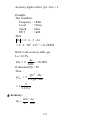
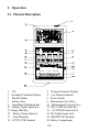
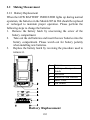
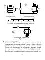
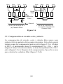
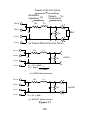
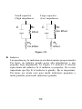
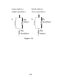
1
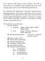
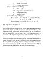
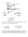
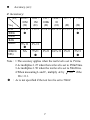
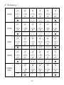
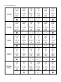
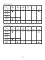
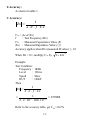
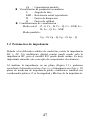
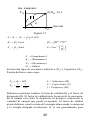
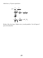
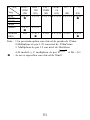
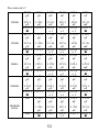
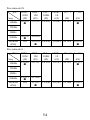
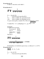
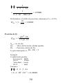
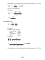
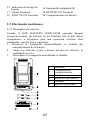
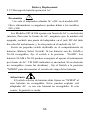
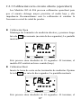
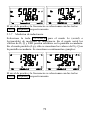
Models 885 & 886 LCR METER OPERATING MANUAL MANUAL DE INSTRUCCIÓNES MEDIDOR LCR Modelos 885 & 886 Contents 1. INTRODUCTION ...............................................................1 1.1 GENERAL............................................................................. 1 1.2 IMPEDANCE PARAMETERS .................................................. 3 1.3 SPECIFICATION .................................................................... 6 1.4 ACCESSORIES ....................................................................19 2. OPERATION ......................................................................21 2.1 PHYSICAL DESCRIPTION ...................................................21 2.2 MAKING MEASUREMENT .................................................21 2.2.1 Battery Replacement ............................................................... 22 2.2.2 Battery Recharging/AC operation .......................................... 23 2.2.3 Open and Short Calibration ................................................... 24 2.2.4 Display Speed .......................................................................... 25 2.2.5 Relative Mode ......................................................................... 25 2.2.6 Range Hold.............................................................................. 25 2.2.7 DC Resistance Measurement .................................................. 26 2.2.8 AC Impedance Measurement .................................................. 26 2.2.9 Capacitance Measurement ..................................................... 26 2.2.10 Inductance Measurement ........................................................ 27 2.3 ACCESSORY OPERATION ...................................................28 4. APPLICATION ..................................................................30 4.1 TEST LEADS CONNECTION ...............................................30 4.2 OPEN/SHORT COMPENSATION ..........................................35 4.3 SELECTING THE SERIES OR PARALLEL MODE ..................37 5. LIMITED THREE-YEAR WARRANTY ......................37 6. SAFETY PRECAUTION .................................................42 1. Introduction 1.1 General The B&K Precision Models 885 & 886 Synthesized In-Circuit LCR/ESR Meter is a high accuracy hand held portable test instrument used for measuring inductors, capacitors and resistors with a basic accuracy of 0.2%. It is the most advanced handheld AC/DC impedance measurement instrument to date. The 885 or 886 can help engineers and students to understand the characteristic of electronics components as well as being an essential tool on any service bench. The instrument is auto or manual ranging. Test frequencies of 100Hz, 120Hz, 1KHz 10KHz or 100KHz (886) may be selected on all applicable ranges. The test voltages of 50mVrms, 0.25Vrms, 1Vrms or 1VDC (DCR only) may also be selected on all applicable ranges. The dual display feature permits simultaneous measurements. Components can be measured in the series or parallel mode as desired; the more standard method is automatically selected first but can be overridden. The Model 885 and 886 offers three useful modes for sorting components. The highly versatile Models can perform virtually all the functions of most bench type LCR bridges. With a basic accuracy of 0.2%, this economical LCR meter may be adequately substituted for a 1 more expensive LCR bridge in many situations. The meter is powered from two AA Batteries and is supplied with an AC to DC charging adapter and two AA Ni-Mh Rechargeable Batteries. The instrument has applications in electronic engineering labs, production facilities, service shops, and schools. It can be used to check ESR values of capacitors, sort values, select precision values, measure unmarked and unknown inductors, capacitors or resistors, and to measure capacitance, inductance, or resistance of cables, switches, circuit board foils, etc. The key features are as following: Test condition: 1 Frequency : 100Hz / 120Hz / 1KHz / 10KHz / 100KHz (886) : 1Vrms / 0.25Vrms / 50mVrms / 2. Level 1VDC (DCR only) Measurement Parameters : Z, Ls, Lp, Cs, Cp, DCR, ESR, D, Q and θ Basic Accuracy: 0.2% Dual Liquid Crystal Display Fast/Slow Measurement Auto Range or Range Hold Open/Short Calibration Primary Parameters Display: Z : AC Impedance DCR : DC Resistance Ls : Serial Inductance Lp : Parallel Inductance 2 Cs : Serial Capacitance Cp : Parallel Capacitance Second Parameter Display: θ : Phase Angle ESR : Equivalence Serial Resistance D : Dissipation Factor Q : Quality Factor Combinations of Display: Serial Mode : Z –θ, Cs – D, Cs – Q, Cs – ESR, Ls – D, Ls – Q, Ls – ESR Parallel Mode : Cp – D, Cp – Q, Lp – D, Lp – Q 1.2 Impedance Parameters Due to the different testing signals on the impedance measurement instrument, there are DC impedance and AC impedance. The common digital multi-meter can only measure the DC impedance, but the Model 885 can do both. It is a very important issue to understand the impedance parameters of the electronic component. When we analysis the impedance by the impedance measurement plane (Figure 1.1). It can be visualized by the real element on the X-axis and the imaginary element on the y-axis. This impedance measurement plane can also be seen as the polar coordinates. The Z is the magnitude and the θ is the phase of the impedance. 3 Imaginary Axis Z (Rs , Xs ) Xs Z θ Rs Real Axis Figure 1.1 Z = Rs + jX s = Z ∠θ (Ω ) Rs = Z Cosθ Z = Rs + X s 2 Xs Rs X s = Z Sinθ θ = Tan −1 2 Z = (Impedance) RS = (Resistance ) X S = (Reactance) Ω = (Ohm ) There are two different types of reactance: Inductive (XL) and Capacitive (XC). It can be defined as follows: X L = ωL = 2πfL 1 = 1 XC = ωC 2πfC L = Inductance (H) C = Capacitance (F) f = Frequency (Hz) Also, there are quality factor (Q) and the dissipation factor (D) that need to be discussed. For component, the quality factor serves as a measure of the reactance purity. In the real world, there is always 4 some associated resistance that dissipates power, decreasing the amount of energy that can be recovered. The quality factor can be defined as the ratio of the stored energy (reactance) and the dissipated energy (resistance). Q is generally used for inductors and D for capacitors. 1 1 = D tan δ X s ωL s 1 = = = Rs Rs ωC s R s B = G Rp Rp = = = ωC p R p X p ωL p Q= There are two types of the circuit mode. One is series mode, the other is parallel mode. See Figure 1.2 to find out the relation of the series and parallel mode. 5 Real and imaginary components are serial Rs jXs Z = Rs + jX s Real and imaginary components are Parallel Rp G=1/Rp jXp jB=1/jXp 1 1 Y= + RP jX P Y = G + jB Figure 1.2 1.3 Specification LCD Display Range: Parameter Z L C DCR ESR D Q θ 0.000 Ω 0.000 µH 0.000 pF 0.000 Ω 0.000 Ω 0.000 0.000 -180.0 ° 6 Range to 9999 MΩ to 9999 H to 9999 F to 9999 MΩ to 9999 Ω to 9999 to 9999 to 180.0 ° Accuracy (Ae): Z Accuracy: |Zx| Freq. DCR 100Hz 120Hz 1KHz 10KHz 100KHz (886) 20M ~ 10M ~ 1M ~ 100K ~ 10 ~ 1 1 ~ 0.1 10M 1M 100K 10 (Ω) (Ω) (Ω) (Ω) (Ω) (Ω) 2% ±1 1% ±1 0.5% ±1 0.2% ±1 0.5% ±1 1% ±1 5% ±1 2% ±1 NA 5%±1 2%±1 0.4% ±1 2%±1 5%±1 Note : 1.The accuracy applies when the test level is set to 1Vrms. 2.Ae multiplies 1.25 when the test level is set to 250mVrms. 3.Ae multiplies 1.50 when the test level is set to 50mVrms. 4.When measuring L and C, multiply Ae by 1+ Dx 2 if the Dx>0.1. : Ae is not specified if the test level is set to 50mV. 7 C Accuracy : 100Hz 120Hz 1KHz 10KHz 79.57 pF | 159.1 pF 2% ± 1 66.31 pF | 132.6 pF 2% ± 1 7.957 pF | 15.91 pF 2% ± 1 0.795 pF | 1.591 pF 5% ± 1 NA 100KHz (886) NA 159.1 pF | 1.591 nF 1% ± 1 132.6 pF | 1.326 nF 1% ± 1 15.91 pF | 159.1 pF 1% ± 1 1.591 pF | 15.91 pF 2% ± 1 0.159 pF | 1.591 pF 5% ± 1 1.591 nF | 15.91 nF 0.5% ±1 1.326 nF | 13.26 nF 0.5% ±1 159.1 pF | 1.591 nF 0.5% ±1 15.91 pF | 159.1 pF 0.5% ±1 1.591 pF | 15.91 pF 2%± 1 8 15.91 nF | 159.1 uF 0.2% ±1 13.26 nF | 132.6 uF 0.2% ±1 1.591 nF | 15.91 uF 0.2% ±1 159.1 pF | 1.591 uF 0.2% ±1 15.91 pF | 159.1 nF 0.4% ±1 159.1 uF | 1591 uF 0.5% ±1 132.6 uF | 1326 uF 0.5% ±1 15.91 uF | 159.1 uF 0.5% ±1 1.591 uF | 15.91 uF 0.5% ±1 159.1 nF | 1.591 uF 2%± 1 1591 uF | 15.91 mF 1% ± 1 1326 uF | 13.26 mF 1% ± 1 159.1 uF | 1.591 mF 1% ± 1 15.91 uF | 159.1 uF 1% ± 1 1.591 uF | 15.91 uF 5% ± 1 L Accuracy : 100Hz 120Hz 1KHz 10KHz 100KHz (886) 31.83 KH | 15.91 KH 2% ± 1 26.52 KH | 13.26 KH 2% ± 1 31.83 KH | 1.591 KH 2% ± 1 318.3 H | 159.1 H 5% ± 1 31.83 H | 15.91 H NA 15.91 KH | 1591 H 1% ± 1 13.26 KH | 1326 H 1% ± 1 1.591 KH | 159.1 H 1% ± 1 159.1 H | 15.91 H 2% ± 1 15.91 H | 1.591 H 5% ± 1 1591 H | 159.1 H 0.5% ±1 1326 H | 132.6 H 0.5% ±1 159.1 H | 15.91 H 0.5% ±1 15.91 H | 1.591 H 0.5% ±1 1.591 H | 159.1 mH 2%± 1 9 159.1 H | 15.91 mH 0.2% ±1 132.6 H | 13.26 mH 0.2% ±1 15.91 H | 1.591 mH 0.2% ±1 1.591 H | 159.1 uH 0.2% ±1 159.1 mH | 15.91 uH 0.4% ±1 15.91 mH | 1.591 mH 0.5% ±1 13.26 mH | 1.326 mH 0.5% ±1 1.591 mH | 159.1 uH 0.5% ±1 159.1 uH | 15.91 uH 0.5% ±1 15.91 uH | 1.591 uH 2%± 1 1.591 mH | 159.1 uH 1% ± 1 1.326 mH | 132.6 uH 1% ± 1 159.1 uH | 15.91 uH 1% ± 1 15.91 uH | 1.591 uH 1% ± 1 1.591 uH | 0.159 uH 5% ± 1 D Accuracy : |Zx| Freq. 100Hz 20M ~ 10M (Ω) ±0.020 10M ~ 1M (Ω) ±0.010 1M ~ 100K (Ω) ±0.005 100K ~ 10 (Ω) ±0.002 10 ~ 1 1 ~ 0.1 (Ω) ±0.005 (Ω) ±0.010 ±0.050 NA ±0.020 ±0.050 ±0.020 ±0.004 ±0.020 ±0.050 20M ~ 10M (Ω) ±1.046 10M ~ 1M (Ω) ±0.523 1M ~ 100K (Ω) ±0.261 100K ~ 10 (Ω) ±0.105 10 ~ 1 1 ~ 0.1 (Ω) ±0.261 (Ω) ±0.523 ±2.615 NA ±1.046 ±1.046 ±0.209 ±1.046 ±2.615 120Hz 1KHz 10KHz 100KHz (886) θ Accuracy : |Zx| Freq. 100Hz 120Hz 1KHz 10KHz 100KHz (886) ±2.615 10 Z Accuracy: As shown in table 1. C Accuracy: Zx = 1 2 ⋅ π ⋅ f ⋅ Cx CAe = Ae of |Zx| f : Test Frequency (Hz) Cx : Measured Capacitance Value (F) |Zx| : Measured Impedance Value (Ω) Accuracy applies when Dx (measured D value) ≦ 0.1 When Dx > 0.1, multiply CAe by 1 + Dx 2 Example: Test Condition: Frequency : 1KHz Level : 1Vrms Speed : Slow DUT : 100nF Then 1 Zx = 2 ⋅ π ⋅ f ⋅ Cx 1 = = 1590Ω 2 ⋅ π ⋅ 103 ⋅ 100 ⋅ 10 − 9 Refer to the accuracy table, get CAe=±0.2% 11 L Accuracy: Zx = 2 ⋅ π ⋅ f ⋅ Lx LAe = Ae of |Zx| f : Test Frequency (Hz) Lx : Measured Inductance Value (H) |Zx| : Measured Impedance Value (Ω) Accuracy applies when Dx (measured D value) ≦ 0.1 When Dx > 0.1, multiply LAe by 1 + Dx 2 Example: Test Condition: Frequency : 1KHz Level : 1Vrms Speed : Slow DUT : 1mH Then Zx = 2 ⋅ π ⋅ f ⋅ Lx = 2 ⋅ π ⋅ 103 ⋅ 10 − 3 = 6.283Ω Refer to the accuracy table, get LAe=±0.5% ESR Accuracy: ESR Ae = ± Xx ⋅ Ae 100 Xx = 2 ⋅ π ⋅ f ⋅ Lx = 1 2 ⋅ π ⋅ f ⋅ Cx 12 ESRAe = Ae of |Zx| f : Test Frequency (Hz) Xx : Measured Reactance Value (Ω) Lx : Measured Inductance Value (H) Cx : Measured Capacitance Value (F) Accuracy applies when Dx (measured D value) ≦ 0.1 Example: Test Condition: Frequency : 1KHz Level : 1Vrms Speed : Slow DUT : 100nF Then 1 Zx = 2 ⋅ π ⋅ f ⋅ Cx 1 = = 1590Ω 3 2 ⋅ π ⋅ 10 ⋅ 100 ⋅ 10 − 9 Refer to the accuracy table, get CAe=±0.2%, Ae ESR Ae = ± Xx ⋅ = ±3.18Ω 100 D Accuracy: D Ae = ± Ae 100 13 DAe = Ae of |Zx| Accuracy applies when Dx (measured D value) ≦ 0.1 When Dx > 0.1, multiply Dx by (1+Dx) Example: Test Condition: Frequency : 1KHz Level : 1Vrms Speed : Slow DUT : 100nF Then 1 Zx = 2 ⋅ π ⋅ f ⋅ Cx 1 = = 1590Ω 3 2 ⋅ π ⋅ 10 ⋅ 100 ⋅ 10 − 9 Refer to the accuracy table, get CAe=±0.2%, Ae D Ae = ± ⋅ = ±0.002 100 Q Accuracy: Q Ae =± 2 Qx ⋅ De 1 Qx ⋅ De QAe = Ae of |Zx| Qx : Measured Quality Factor Value De : Relative D Accuracy 14 Accuracy applies when Qx ⋅ De < 1 Example: Test Condition: Frequency : 1KHz Level : 1Vrms Speed : Slow DUT : 1mH Then Zx = 2 ⋅ π ⋅ f ⋅ Lx = 2 ⋅ π ⋅ 103 ⋅ 10 − 3 = 6.283Ω Refer to the accuracy table, get LAe=±0.5%, Ae De = ± ⋅ = ±0.005 100 If measured Qx = 20 Then Qx 2 ⋅ De Q Ae = ± 1 Qx ⋅ De 2 =± 1 0.1 θ Accuracy: θe = 180 Ae ⋅ π 100 15 Example: Test Condition: Frequency : 1KHz Level : 1Vrms Speed : Slow DUT : 100nF Then 1 Zx = 2 ⋅ π ⋅ f ⋅ Cx 1 = = 1590Ω 3 2 ⋅ π ⋅ 10 ⋅ 100 ⋅ 10 − 9 Refer to the accuracy table, get ZAe=±0.2%, 180 Ae θ Ae = ± ⋅ π 100 180 0.2 =± ⋅ = ±0.115 deg π 100 Testing Signal: Level Accuracy Frequency Accuracy : ± 5% : 0.1% Output Impedance : 100Ω ± 5% Measuring Speed: Fast : 4.5 meas. / sec. Slow : 2.5 meas. / sec. 16 General: Temperature : 0°C to 70°C (Operating) -20°C to 70°C (Storage) Relative Humidity : Up to 85% Battery Type : 2 AA size Ni-Mh or Alkaline Battery Charge : Constant current 150mA approximately Battery Operating Time : 2.5 Hours typical AC Operation : 110/220V AC, 60/50Hz with proper adapter Low Power Warning : under 2.2V Dimensions : 174mm x 86mm x 48mm (L x W x H) 6.9” x 3.4” x 1.9” Weight : 470g Considerations Test Frequency. The test frequency is user selectable and can be changed. Generally, a 1 KHz test signal or higher is used to measure capacitors that are 0.01uF or smaller and a 120Hz test signal is used for capacitors that are 10uF or larger. Typically a 1 kHz test signal or higher is used to measure inductors that are used in audio and RF (radio frequency) circuits. This is because these components operate at higher frequencies and require that they be measured at a higher frequency of 1 KHz. Generally, inductors below 2mH should be measured at 1 kHz and inductors above 200H should be measured at 120Hz. It is best to check with the component manufacturers’ data sheet to determine the best test frequency for the device. 17 Charged Capacitors Always discharge any capacitor prior to making a measurement since a charged capacitor may seriously damage the meter. Effect Of High D on Accuracy A low D (Dissipation Factor) reading is desirable. Electrolytic capacitors inherently have a higher dissipation factor due to their normally high internal leakage characteristics. If the D (Dissipation Factor) is excessive, the capacitance measurement accuracy may be degraded. It is best to check with the component manufacturers’ data sheet to determine the desirable D value of a good component. Measuring Capacitance of Cables, Switches or Other Parts Measuring the capacitance of coaxial cables is very useful in determining the actual length of the cable. Most manufacturer specifications list the amount of capacitance per foot of cable and therefore the length of the cable can be determined by measuring the capacitance of that cable. For example: A manufacturers, specification calls out a certain cable, to have a capacitance of 10 pF per foot, After measuring the cable a capacitance reading of 1.000 nF is displayed. Dividing 1000pF (1.000 nF) by 10 pF per foot yields the length of the cable to be approximately 100 feet. 18 Even if the manufacturers’ specification is not known, the capacitance of a measured length of cable (such as 10 feet) can be used to determine the capacitance per foot; do not use too short a length such as one foot, because any error becomes magnified in the total length calculations. Sometimes, the capacitance of switches, interconnect cables, circuit board foils, or other parts, affecting stray capacitance can be critical to circuit design, or must be repeatable from one unit to another. Series Vs Parallel Measurement (for Inductors) The series mode displays the more accurate measurement in most cases. The series equivalent mode is essential for obtaining an accurate Q reading of low Q inductors. Where ohmic losses are most significant, the series equivalent mode is preferred. However, there are cases where the parallel equivalent mode may be more appropriate. For iron core inductors operating at higher frequencies where hysteresis and eddy currents become significant, measurement in the parallel equivalent mode is preferred. 1.4 Accessories Operating Manual 2 AA Size Ni-Mh Rechargeable Batteries Shorting Bar AC to DC Adapter TL885A SMD Test Probe TL885B 4-Wire Test Clip (Optional) TL08C Kelvin Clip (Optional) 19 1 pc 2 pc 1 pc 1 pc 1 pc Carrying Case (Optional) 20 2. Operation 2.1 Physical Description 1. 3. 5. 7. 9. 11. 13. 15. 17. 19. G UARD H POT L POT H CUR L CUR G UARD NA Secondary Parameter Display Model Number Relative Key Open/Short Calibration Key Display Update Speed Key Range Hold Key Battery Charge Indicator Guard Terminal LPOT/LCUR Terminal 2. 4. 6. 8. 10. 12. 14. 16. 18. 20. Primary Parameter Display Low Battery Indicator Power Switch Measurement Level Key Measurement Frequency Key D/Q/θ/ESR Function Key L/C/Z/DCR Function Key DC Adapter Input Jack HPOT/HCUR Terminal Battery Compartment 21 2.2 Making Measurement 2.2.1 Battery Replacement When the LOW BATTERY INDICATOR lights up during normal operation, the batteries in the Models 885 & 886 should be replaced or recharged to maintain proper operation. Please perform the following steps to change the batteries: 1. Remove the battery hatch by unscrewing the screw of the battery compartment. 2. Take out the old batteries and insert the new batteries into the battery compartment. Please watch out for battery polarity when installing new batteries. 3. Replace the battery hatch by reversing the procedure used to remove it. 1 2 3 4 5 6 Screws Battery Compartment Hatch Batteries Norm/Ni-Mh Switch Back Case Tilt Stand Battery Replacement 22 2.2.2 Battery Recharging/AC operation Caution ! Only the Models 885 or 886 standard accessory AC to DC adapter can be used with Model 885. Other battery eliminator or charger may result in damage to Modes 885 or 886. The Models 885 & 886 works on external AC power or internal batteries. To power the Model 885 with AC source, make sure that the Models 885 or 886 is off, then plug one end of the AC to DC adapter into the DC jack on the right side of the instrument and the other end into an AC outlet. There is a small slide switch inside the battery compartment called Battery Select Switch. If the Ni-Mh or Ni-Cd rechargeable batteries are installed in Models 885 or 886, set the Battery Select Switch to "Ni-Mh" position. The Ni-Mh or Ni-Cd batteries can be recharged when the instrument is operated by AC source. The LED for indicating battery charging will light on. If the non-rechargeable batteries (such as alkaline batteries) are installed in Models 885 or 886, set the Battery Select Switch to "NORM" position for disconnecting the charging circuit to the batteries. Warning The Battery Select Switch must be set in the "NORM" position when using non-rechargeable batteries. Non-rechargeable batteries may explode if the AC adapter is used with non-rechargeable batteries. Warranty is voided if this happened. 23 2.2.3 Open and Short Calibration The Models 885 & 886 provides open/short calibration capability so the user can get better accuracy in measuring high and low impedance. We recommend that the user performs open/short calibration if the test level or frequency has been changed. Open Calibration First, remaining the measurement terminals with the open status, then press the CAL key shortly (no more than two second), the LCD will display: This calibration takes about 10 seconds. After it is finished, the Model 885 will beep to show that the calibration is done. Short Calibration To perform the short calibration, insert the Shorting Bar into the measurement terminals. Press the CAL key for more than two second, the LCD will display: This calibration takes about 10 seconds. After it is finished, the Model 885 will beep to show that the calibration is done. 24 2.2.4 Display Speed The Models 885 & 886 provides two different display speeds (Fast/Slow). It is controlled by the Speed key. When the speed is set to fast, the display will update 4.5 readings every second. When the speed is set to slow, it’s only 2.5 readings per second. 2.2.5 Relative Mode The relative mode lets the user to make quick sort of a bunch of components. First, insert the standard value component to get the standard value reading. (Approximately 5 seconds in Fast Mode to get a stable reading.) Then, press the Relative key, the primary display will reset to zero. Remove the standard value component and insert the unknown component, the LCD will show the value that is the difference between the standard value and unknown value. 2.2.6 Range Hold To set the range hold, insert a standard component in that measurement range. (Approximately 5 seconds in Fast Mode to get a stable reading.) Then, by pressing the Range Hold key it will hold the range within 0.5 to 2 times of the current measurement range. When the Range Hold is press the LCD display: 25 2.2.7 DC Resistance Measurement The DC resistance measurement measures the resistance of an unknown component by 1VDC. Select the L/C/Z/DCR key to make the DCR measurement. The LCD display: 2.2.8 AC Impedance Measurement The AC impedance measurement measures the Z of an unknown device. Select the L/C/Z/DCR key to make the Z measurement. The LCD display: The testing level and frequency can by selected by pressing the Level key and Frequency key, respectively. 2.2.9 Capacitance Measurement To measure the capacitance of a component, select the L/C/Z/DCR key to Cs or Cp mode. Due to the circuit structure, there are two modes can by selected (Serial Mode – Cs and Parallel Mode – Cp). If the serial mode (Cs) is selected, the D, Q and ESR can be shown on the secondary display. If the parallel mode (Cp) is selected, only the D and Q can be shown on the secondary display. The following 26 shows some examples of capacitance measurement: The testing level and frequency can by selected by pressing the Level key and Frequency key, respectively. 2.2.10 Inductance Measurement Select the L/C/Z/DCR key to Ls or Lp mode for measuring the inductance in serial mode or parallel mode. If the serial mode (Ls) is selected, the D, Q and ESR can be shown on the secondary display. If the parallel mode (Lp) is selected, only the D and Q can be shown on the secondary display. The following shows some examples of capacitance measurement: The testing level and frequency can by selected by pressing the Level key and Frequency key, respectively. 27 2.3 Accessory Operation Follow the figures below to attach the test probes for making measurement. Shorting Bar TL885A SMD Test Probe 28 HP LP LC HC TL885B 4-Wire Test Clip TL08C Kelvin Clip 29 4. Application 4.1 Test Leads Connection Auto balancing bridge has four terminals (HCUR, HPOT, LCUR and LPOT) to connect to the device under test (DUT). It is important to understand what connection method will affect the measurement accuracy. 2-Terminal (2T) 2-Terminal is the easiest way to connect the DUT, but it contents many errors which are the inductor and resistor as well as the parasitic capacitor of the test leads (Figure 3.1). Due to these errors in measurement, the effective impedance measurement range will be limited at 100Ω to 10KΩ. Ro Lo A HCUR HPOT DUT Co V LPOT LCUR Ro (a) CONNECTION Lo (b) BLOCK DIAGRAM 2T 1m 10m 100m 1 10 100 1K 10K 100K 1M 10M (c) TYPICAL IMPEDANCE MEASUREMENT RANGE(£[) Figure 3.1 3-Terminal (3T) 30 DUT 3-Terminal uses coaxial cable to reduce the effect of the parasitic capacitor (Figure 3.2). The shield of the coaxial cable should connect to guard of the instrument to increase the measurement range up to 10MΩ. Ro Lo A HCUR HPOT DUT Co V DUT Co doesn't effect measurement result LPOT LCUR Ro (a) CONNECTION Lo (b) BLOCK DIAGRAM 3T 1m 10m 100m 1 10 100 1K 10K 100K 1M 10M (c) TYPICAL IMPEDANCE MEASUREMENT RANGE(£[) A V DUT (d) 2T CONNECTION WITH SHILDING Figure 3.2 4-Terminal (4T) 4-Terminal connection reduces the effect of the test lead 31 resistance (Figure 3.3). This connection can improve the measurement range down to 10mΩ. However, the effect of the test lead inductance can’t be eliminated. A HCUR HPOT DUT V DUT LPOT LCUR (a) CONNECTION (b) BLOCK DIAGRAM 4T 1m 10m 100m 1 10 100 1K 10K 100K 1M 10M (c) TYPICAL IMPEDANCE MEASUREMENT RANGE (£[) Figure 3.3 5-Terminal (5T) 5-Terminal connection is the combination of 3T and 4T (Figure 3.4). It has four coaxial cables. Due to the advantage of the 3T and 4T, this connection can widely increase the measurement range for 10mΩ to 10MΩ. 32 A HCUR HPOT DUT V DUT LPOT L CUR (a) CONNECTION (b) BLOCK DIAGRAM 5T 1m 10m 100m 1 10 100 1K 10K 100K 1M 10M (c) TYPICAL IMPEDANCE MEASUREMENT RANGE (£[) A V DUT (d) WRONG 4T CONNECTION Figure 3.4 4-Terminal Path (4TP) 4-Terminal Path connection solves the problem that caused by the test lead inductance. 4TP uses four coaxial cables to isolate the current path and the voltage sense cable (Figure 3.5). The return current will flow through the coaxial cable as well as the shield. Therefore, the magnetic flux that generated by internal conductor will cancel out the magnetic flux generated by external conductor (shield). The 4TP connection increases the 33 measurement range from 1mΩ to 10MΩ. HCUR V HPOT DUT DUT LPOT LCUR A (a) CONNECTION (b) BLOCK DIAGRAM HCUR HPOT 4T DUT LPOT 1m 10m 100m 1 10 100 1K 10K 100K 1M 10M (c) TYPICAL IMPEDANCE MEASUREMENT RANGE(£[) LCUR (d) 4T CONNECTION WITH SHILDING Figure 3.5 Eliminating the Effect of the Parasitic Capacitor When measuring the high impedance component (i.e. low capacitor), the parasitic capacitor becomes an important issue (Figure 3.6). In figure 3.6(a), the parasitic capacitor Cd is paralleled to DUT as well as the Ci and Ch. To correct this problem, add a guard plane (Figure 3.6(b)) in between H and L terminals to break the Cd. If the guard plane is connected to instrument guard, the effect of Ci and Ch will be removed. 34 HCUR HPOT LPOT LCUR Cd HPOT LPOT LCUR Guard Plant DUT Ch HCUR Connection Point Cl Ground (b) Guard Plant reduces Parastic Effect (a) Parastic Effect Figure 3.6 4.2 Open/Short Compensation For those precision impedance measuring instrument, the open and short compensation need to be used to reduce the parasitic effect of the test fixture. The parasitic effect of the test fixture can be treated like the simple passive components in figure 3.7(a). When the DUT is open, the instrument gets the conductance Yp = Gp + jωCp (Figure 3.7(b)). When the DUT is short, the instrument gets the impedance Zs = Rs + jωLs (Figure 3.7(c)). After the open and short compensation, Yp and Zs are for calculating the real Zdut (Figure 3.7(d)). 35 Parastic of the Test Fixture Redundant (Zs) Impedance HCUR Rs Parastic (Yo) Conductance Ls HPOT Zm Co Zdut Go LPOT LCUR (a) Parastic Effect of the Test Fixture HCUR Rs Ls HPOT Yo Co Go OPEN LPOT LCUR Yo = Go + j£sCo 1 (Rs + j£s<< ) Go+j£sCo (b) OPEN Measurement HCUR Rs Ls HPOT Zs Co LPOT LCUR Zs = Rs + j£sLs (c) SHORT Measurement Figure 3.7 36 Go SHORT Zs Zm Yo Zdut Zdut = Zm - Zs 1-(Zm-Zs)Yo (d) Compensation Equation Figure 3.7 (Continued) 4.3 Selecting the Series or Parallel Mode According to different measuring requirement, there are series and parallel modes to describe the measurement result. It is depending on the high or low impedance value to decide what mode to be used. Capacitor The impedance and capacitance in the capacitor are negatively proportional. Therefore, the large capacitor means the low impedance; the small capacitor means the high impedance. Figure 3.8 shows the equivalent circuit of capacitor. If the capacitor is small, the Rp is more important than the Rs. If the capacitor is large, the Rs shouldn’t be avoided. Hence, uses parallel mode to measure low capacitor and series mode to measure high capacitor. 37 Small capacitor (High impedance) C RP Large capacitor (Low impedance) C RP No Effect Effect RS RS No Effect Effect Figure 3.8 Inductor The impedance and inductive in the inductor are positively proportional. Therefore, the large inductor equals to the high impedance and vice versa. Figure 3.9 shows the equivalent circuit of inductor. If the inductor is small, the Rs is more important than the Rp. If the inductor is large, the Rp should be taking care of. So, uses series mode to measure low inductor and parallel mode to measure high inductor. 38 Large inductor (High impedance) Small inductor (Low impedance) L L RP RP No Effect Effect RS RS No Effect Effect Figure 3.9 39 5. Limited Three-Year Warranty B&K Precision Corp. warrants to the original purchaser that its products and the component parts thereof, will be free from defects in workmanship and materials for a period of three years from date of purchase. B&K Precision Corp. will, without charge, repair or replace, at its option, defective product or component parts. Returned product must be accompanied by proof of the purchase date in the form of a sales receipt. To obtain warranty coverage in the U.S.A., this product must be registered by completing a warranty registration form on our website www.bkprecision.com within fifteen (15) days of purchase. Exclusions: This warranty does not apply in the event of misuse or abuse of the product or as a result of unauthorized alternations or repairs. It is void if the serial number is alternated, defaced or removed. B&K Precision Corp. shall not be liable for any consequential damages, including without limitation damages resulting from loss of use. Some states do not allow limitation of incidental or consequential damages, so the above limitation or exclusion may not apply to you. This warranty gives you specific rights and you may have other rights, which vary from state-to-state. 40 Service Information Warranty Service: Please return the product in the original packaging with proof of purchase to the below address. Clearly state in writing the performance problem and return any leads, connectors and accessories that you are using with the device. Non-Warranty Service: Return the product in the original packaging to the below address. Clearly state in writing the performance problem and return any leads, connectors and accessories that you are using with the device. Customers not on open account must include payment in the form of a money order or credit card. For the most current repair charges contact the factory before shipping the product. Return all merchandise to B&K Precision Corp. with pre-paid shipping. The flat-rate repair charge includes return shipping to locations in North America. For overnight shipments and non-North America shipping fees contact B&K Precision Corp.. B&K Precision Corp. 22820 Savi Ranch Parkway Yorba Linda, CA 92887 Phone: 714- 921-9095 Email: [email protected] Include with the instrument your complete return shipping address, contact name, phone number and description of problem. 41 6. Safety Precaution SAFETY CONSIDERATIONS The Models 885 & 886 LCR Meter has been designed and tested according to Class 1A 1B or 2 according to IEC479-1 and IEC 721-3-3, Safety requirement for Electronic Measuring Apparatus. SAFETY PRECAUTIONS SAFETY NOTES The following general safety precautions must be observed during all phases of operation, service, and repair of this instrument. Failure to comply with these precautions or with specific warnings elsewhere in this manual violates safety standards of design, manufacture, and intended use of the instrument. The manufacturer assumes no liability for the customer‘s failure to comply with these requirements. BEFORE APPLYING POWER ! Verify that the product is set to match the available line voltage is installed. 42 SAFETY SYMBOLS Caution, risk of electric shock Earth ground symbol Equipment protected throughout by double insulation or reinforced insulation ! Caution (refer to accompanying documents) DO NOT SUBSTITUTE PARTS OR MODIFY INSTRUMENT Because of the danger of introducing additional hazards, do not install substitute parts or perform any unauthorized modification to the instrument. Return the instrument to a qualified dealer for service and repair to ensure that safety features are maintained. INSTRUMENTS WHICH APPEAR DAMAGED OR DEFECTIVE SHOULD NOT BE USED! PLEASE CONTACT B&K PRECISION FOR INFORMATION ON REPAIRS. 43 Tabla de Contendido 1. INTRODUCCIÓN ............................................................. 45 GENERAL .......................................................................... 45 PARÁMETROS DE IMPEDANCIA ......................................... 47 ESPECIFICACIÓN ............................................................... 50 ACCESSORIOS ................................................................... 63 2. OPERACIÓN ..................................................................... 64 2.1 DESCRIPCIÓN FÍSICA ......................................................... 64 2.2 EFECTUANDO MEDICIONES ................................................... 65 1.1 1.2 1.3 1.4 2.1.1 Reemplazo de baterías ............................................................ 65 2.1.2 Recarga de batería/operación AC.......................................... 66 2.1.3 Calibración/corto circuito abierto (open/short) .................... 67 2.1.4 Velocidad de visualización ..................................................... 69 2.1.5 Modo relativo .......................................................................... 69 2.1.6 Retención de rango ................................................................. 69 2.1.7 Medición de resistencia DC ................................................... 69 2.1.8 Medición de impedancia AC .................................................. 70 2.1.9 Medición de Capacitancia...................................................... 70 2.1.10 Medición de inductancia ........................................................ 71 2.2 OPERACIÓN DE LOS ACCESORIOS ..................................... 72 3. APLICACIÓN .................................................................... 74 3.1 CONEXIÓN DE LAS PUNTAS DE PRUEBA ........................... 74 3.2 COMPENSACIÓN EN CIRCUITO CORTO Y ABIERTO ............ 79 3.3 SELECCIÓN DEL MODO SERIAL O PARALELO .................... 81 5. PRECAUCIÓN SOBRE SEGURIDAD ......................... 84 44 1. Introducción 1.1 General Los Modelos 885 & 886 de B&K Precision,Medidor LCR/ESR en circuito es un instrumento portátil de alta precisión para medir inductores, capacitores y resistores con una precisión del 0.5%. Es el instrumento portátil más avanzado a la fecha. El 885 u 886 puede ayudar a ingenieros y estudiantes a comprender las componentes y a efectuar servicio de equipos en el taller electrónico. Los rangos del instrumento pueden ser automáticos o manuales. En todos los rangos puede seleccionar frecuencias de 100Hz, 120Hz, 1KHz 10KHz o 100KHz (886). Puede seleccionar voltajes de prueba de 50mVrms, 0.25Vrms, 1Vrms o 1VDC (DCR solamente) en todos los rangos. La pantalla doble permite mediciones simultáneas. Los componentes pueden medirse en modo serial o paralelo; el método estándar se selecciona primero pero puede cambiarse. Los Modelos 885 y 886 ofrecen tres modos útiles para ordenar componentes. 45 Estos versátiles modelos pueden realizar virtualmente todas las funciones de puentes LCR. Este económico medidor puede sustituIr a un Puente LCR, con una precisión básica del 0.2%. Opera con dos baterías AA y se entrega con un adaptador cargador AC a DC y dos baterías AA Ni-Mh recargables. El instrumento se emplea en escuelas, laboratorios, líneas de producción y talleres de servicio. Verifica valores ESR, ordena valores, selecciona valores de precisión, mide inductores de valor desconocido, capacitores o resistores, y permite medir capacitancia, inductancia o resistencia de cables, switches, tablillas de circuito impreso, etc. Las caracteristicas principales son: Condición de prueba: 2 Frecuencia : 100Hz / 120Hz / 1KHz / 10KHz / 100KHz (886) 3. Nivel : 1Vrms / 0.25Vrms / 50mVrms / 1VDC (DCR solamente) Parámetros de medición : Z, Ls, Lp, Cs, Cp, DCR, ESR, D, Q y θ Precisión básica: 0.2% Pantalla LCD dual Medición rápida/lenta Rango automático o retención Interfaz infrarroja Calibración en corto/circuito abierto Visualización de parámetros primarios: Z : Impedancia AC DCR : Resistencia DC Ls : Inductancia serial Lp : Inductancia paralelo Cs : Capacitancia serial 46 Cp : Capacitancia paralelo Visualización de parámetro secundario: θ : Angulo de fase ESR : Resistencia serial equivalente D : Factor de disipación Q : Factor de calidad Combinaciones de visualización : Modo serial : Z –θ, Cs – D, Cs – Q, Cs – ESR, Ls – D, Ls – Q, Ls – ESR Modo paralelo : Cp – D, Cp – Q, Lp – D, Lp – Q 1.2 Parámetros de impedancia Debido a las diferentes señales de medición, existe la impedancia DC y AC. Un multímetro digital común puede medir solo la impedancia DC, pero el modelo 885 puede medir ambas. Es muy importante entender este concepto de componentes electrónicas. Al analizar la impedancia en un plano (Figura 1.1), podemos visualizar el elemento real en el eje x y el imaginario en el eje y. El plano de medición de impedancia puede visualizarse también con coordenadas polares: Z es la magnitud y θla fase de la impedancia. 47 Eje imaginario Z (Rs , Xs ) Xs Z θ Rs Eje real Figura 1.1 Z = Rs + jX s = Z ∠θ (Ω ) Rs = Z Cosθ Z = Rs + X s 2 Xs Rs X s = Z Sinθ θ = Tan −1 2 Z = (Impedance) RS = (Resistance) X S = (Reactance) Ω = (Ohm ) Existen dos tipos de reactancia: Inductiva (XL) y Capacitiva (XC). Pueden definirse como sigue X L = ωL = 2πfL 1 = 1 XC = ωC 2πfC L = Inductance (H) C = Capacitance (F) f = Frequency (Hz) Debemos considerar también el factor de calidad (Q) y el factor de disipación (D). El factor de calidad mide la pureza de la reactancia. En el mundo real existe la disipación de potencia, reduciendo la cantidad de energía que puede recuperarse. El factor de calidad puede definirse como la razón de la energía almacenada (reactancia) y la energía disipada (resistencia). Q se usa generalmente para 48 inductores y D para capacitores. 1 1 = D tan δ X s ωL s 1 = = = Rs Rs ωC s R s B = G Rp Rp = = = ωC p R p X p ωL p Q= Modos. Hay dos tipos: Modo serie y modo paralelo. Vea la Figura 2 para relacionarlos. 49 Los componentes real e imaginario son seriales Rs jXs Z = Rs + jX s Los componentes real e imaginario son paralelos Rp G=1/Rp jXp jB=1/jXp 1 1 Y= + RP jX P Y = G + jB Figura 1.2 1.3 Especificación Rango de pantalla LCD: Parámetro Z L C DCR ESR D Q θ Precisión(Ae): 0.000Ω 0.000µH 0.000pF 0.000Ω 0.000Ω 0.000 0.000 -180.0° Precisión de Z: 50 Rango to 9999MΩ to 9999H to 9999F to 9999MΩ to 9999Ω to 9999 to 9999 to 180.0° |Zx| Freq. DCR 100Hz 120Hz 1KHz 10KHz 100KHz (886) 20M ~ 10M (Ω) 2% ±1 10M ~ 1M ~ 100K ~ 10 ~ 1 1 ~ 0.1 1M 100K 10 (Ω) (Ω) (Ω) (Ω) (Ω) 1% ±1 0.5% ±1 0.2% ±1 0.5% ±1 1% ±1 5% ±1 NA 2% ±1 5%±1 2%±1 0.4% ±1 2%±1 5%±1 Note : 1.La precisión aplica con el nivel de prueba de 1Vrms. 2.Multiplicar Ae por 1.25 con nivel de 250mVrms. 3. Multiplicar Ae por 1.5 con nivel de 50mVrms. 4.Al medir L y C, multiplicar Ae por 1+ Dx : Ae no se especifica con el nivel de 50mV. 51 2 si Dx>0.1. Precisión de C: 100Hz 120Hz 1KHz 10KHz 79.57 pF | 159.1 pF 2% ± 1 66.31 pF | 132.6 pF 2% ± 1 7.957 pF | 15.91 pF 2% ± 1 0.795 pF | 1.591 pF 5% ± 1 NA 100KHz (886) NA 159.1 pF | 1.591 nF 1% ± 1 132.6 pF | 1.326 nF 1% ± 1 15.91 pF | 159.1 pF 1% ± 1 1.591 pF | 15.91 pF 2% ± 1 0.159 pF | 1.591 pF 5% ± 1 1.591 nF | 15.91 nF 0.5% ±1 1.326 nF | 13.26 nF 0.5% ±1 159.1 pF | 1.591 nF 0.5% ±1 15.91 pF | 159.1 pF 0.5% ±1 1.591 pF | 15.91 pF 2%± 1 52 15.91 nF | 159.1 uF 0.2% ±1 13.26 nF | 132.6 uF 0.2% ±1 1.591 nF | 15.91 uF 0.2% ±1 159.1 pF | 1.591 uF 0.2% ±1 15.91 pF | 159.1 nF 0.4% ±1 159.1 uF | 1591 uF 0.5% ±1 132.6 uF | 1326 uF 0.5% ±1 15.91 uF | 159.1 uF 0.5% ±1 1.591 uF | 15.91 uF 0.5% ±1 159.1 nF | 1.591 uF 2%± 1 1591 uF | 15.91 mF 1% ± 1 1326 uF | 13.26 mF 1% ± 1 159.1 uF | 1.591 mF 1% ± 1 15.91 uF | 159.1 uF 1% ± 1 1.591 uF | 15.91 uF 5% ± 1 Precisión de L: 31.83 KH | 15.91 100Hz KH 2% ± 1 26.52 KH | 13.26 120Hz KH 2% ± 1 31.83 KH | 1.591 1KHz KH 2% ± 1 318.3 H | 159.1 10KHz H 5% ± 1 31.83 H | 100KHz 15.91 (886) H NA 15.91 KH | 1591 H 1% ± 1 13.26 KH | 1326 H 1% ± 1 1.591 KH | 159.1 H 1% ± 1 159.1 H | 15.91 H 2% ± 1 15.91 H | 1.591 H 5% ± 1 1591 H | 159.1 H 0.5% ±1 1326 H | 132.6 H 0.5% ±1 159.1 H | 15.91 H 0.5% ±1 15.91 H | 1.591 H 0.5% ±1 1.591 H | 159.1 mH 2%± 1 53 159.1 H | 15.91 mH 0.2% ±1 132.6 H | 13.26 mH 0.2% ±1 15.91 H | 1.591 mH 0.2% ±1 1.591 H | 159.1 uH 0.2% ±1 159.1 mH | 15.91 uH 0.4% ±1 15.91 mH | 1.591 mH 0.5% ±1 13.26 mH | 1.326 mH 0.5% ±1 1.591 mH | 159.1 uH 0.5% ±1 159.1 uH | 15.91 uH 0.5% ±1 15.91 uH | 1.591 uH 2%± 1 1.591 mH | 159.1 uH 1% ± 1 1.326 mH | 132.6 uH 1% ± 1 159.1 uH | 15.91 uH 1% ± 1 15.91 uH | 1.591 uH 1% ± 1 1.591 uH | 0.159 uH 5% ± 1 Precisión de D: |Zx| Freq. 100Hz 20M ~ 10M ~ 1M ~ 100K ~ 10 ~ 1 1 ~ 0.1 10M 1M 100K 10 (Ω) (Ω) (Ω) (Ω) (Ω) (Ω) ±0.020 ±0.010 ±0.005 ±0.002 ±0.005 ±0.010 120Hz 1KHz 10KHz 100KHz (886) ±0.050 ±0.020 NA ±0.050 ±0.020 ±0.004 ±0.020 ±0.050 Precisión de θ : |Zx| Freq. 100Hz 20M ~ 10M ~ 1M ~ 100K ~ 10 ~ 1 1 ~ 0.1 10M 1M 100K 10 (Ω) (Ω) (Ω) (Ω) (Ω) (Ω) ±1.046 ±0.523 ±0.261 ±0.105 ±0.261 ±0.523 120Hz 1KHz 10KHz 100KHz (886) ±2.615 ±1.046 NA ±2.615 ±1.046 ±0.209 ±1.046 ±2.615 54 Precisión de Z: Como se muestra en la tabla 1. Precisión de C: Zx = 1 2 ⋅ π ⋅ f ⋅ Cx CAe = Ae de |Zx| f : Frecuencia de prueba (Hz) Cx : Valor medido de capacitancia (F) |Zx| : Valor medido de impedancia (Ω) La precisión aplica cuando Dx (Valor medido D ) ≦ 0.1 Cuando Dx > 0.1, multiplique CAe por 1 + Dx 2 Ejemplo: Condición de prueba: Frecuencia : 1KHz Nivel : 1Vrms Velocidad : Lenta DUT : 100nF Entonces 1 2 ⋅ π ⋅ f ⋅ Cx 1 = = 1590Ω 3 2 ⋅ π ⋅ 10 ⋅ 100 ⋅ 10 − 9 Zx = Refiriéndose a la tabla de precision, se obtiene CAe=±0.2% Precisión de L: Zx = 2 ⋅ π ⋅ f ⋅ Lx LAe = Ae de |Zx| f : Frecuencia de prueba (Hz) 55 Lx : Valor medido de inductancia (H) |Zx| : Valor medido de imperdancia(Ω) La precisión aplica cuando Dx (Valor medido D ) ≦ 0.1 Cuando Dx > 0.1, multiplique CAe por 1 + Dx 2 Ejemplo: Condición de prueba: Frecuencia : 1KHz Nivel : 1Vrms Velocidad : Lenta DUT : 1mH Entonces Zx = 2 ⋅ π ⋅ f ⋅ Lx = 2 ⋅ π ⋅ 103 ⋅ 10 − 3 = 6.283Ω Refiriéndose a la tabla de precisión, obtenemos LAe=±0.5% Precisión ESR: ESR Ae = ± Xx ⋅ Ae 100 Xx = 2 ⋅ π ⋅ f ⋅ Lx = 1 2 ⋅ π ⋅ f ⋅ Cx ESRAe = Ae de |Zx| f : Frecuencia de prueba (Hz) Xx : Valor medido de reactancia (Ω) Lx : Valor medido de inductancia (H) Cx : Valor medido de capacitancia (F) 56 La precisión aplica cuando Dx ≦ 0.1 Ejemplo: Condición de prueba: Frecuencia : 1KHz Nivel : 1Vrms Velocidad : Lenta DUT : 100nF Entonces 1 2 ⋅ π ⋅ f ⋅ Cx 1 = = 1590Ω 3 2 ⋅ π ⋅ 10 ⋅ 100 ⋅ 10 − 9 Zx = Refiriéndose a la tabla, obtenemos CAe=±0.2%, ESR Ae = ± Xx ⋅ Ae = ±3.18Ω 100 Precisión D: D Ae = ± Ae 100 DAe = Ae of |Zx| La precisión aplica cuando Dx (Valor medido D ) ≦ 0.1 Cuando Dx > 0.1, multiplique DAe por (1+Dx) Ejemplo: Condición de prueba: Frecuencia : 1KHz Nivel : 1Vrms Velocidad : Lenta DUT : 100nF Entonces 57 1 2 ⋅ π ⋅ f ⋅ Cx 1 = = 1590Ω 3 2 ⋅ π ⋅ 10 ⋅ 100 ⋅ 10 − 9 Zx = Refiriéndose a la tabla de precisión, obtenemos CAe=±0.2%, D Ae = ± ⋅ Ae = ±0.002 100 Precisión de Q: Q Ae =± 2 Qx ⋅ De 1 Qx ⋅ De QAe = Ae de |Zx| Qx : Valor del factor de calidad medido De : Precisión relativa de De La precisión aplica si Qx ⋅ De < 1 Ejemplo: Condición de prueba: Frecuencia : 1KHz Nivel : 1Vrms Velocidad : Lenta DUT : 1mH Entonces Zx = 2 ⋅ π ⋅ f ⋅ Lx = 2 ⋅ π ⋅ 103 ⋅ 10 − 3 = 6.283Ω 58 Refiriéndose a la tabla de precisión, obtenemos LAe=±0.5%, De = ± ⋅ Ae = ±0.005 100 Si Qx = 20 (medido) Entonces Q Ae = ± =± Qx 2 ⋅ De 1 Qx ⋅ De 2 1 0.1 Precisión de θ : θe = 180 Ae ⋅ π 100 Ejemplo: Condición de prueba: Frecuencia: 1KHz Nivel : 1Vrms Velocidad : Lenta DUT : 100nF Entonces 1 2 ⋅ π ⋅ f ⋅ Cx 1 = = 1590Ω 3 2 ⋅ π ⋅ 10 ⋅ 100 ⋅ 10 − 9 Zx = Refiriéndose a la tabla de precisión, obtenemos ZAe=±0.2%, 59 180 Ae ⋅ π 100 180 0.2 =± ⋅ = ±0.115 deg π 100 θ Ae = ± Señal de prueba: Precisión del nivel : ± 5% Precisión de la frecuencia : 0.1% Impedancia de salida : 100Ω ± 5% Velocidad de medición: Rápida : 4.5 meas. / sec. Lenta : 2.5 meas. / sec. General: Temperatura : 0°C to 70°C (Operativa) -20°C to 70°C (Almacenamiento) Humedad relativa : Hasta 85% Batería : 2 AA Ni-Mh o Alcalina Carga de batería : Corriente constante 150mA aproximada Tiempo de operación : 2.5 Horas típica Operación AC : 110/220V AC, 60/50Hz con adaptador apropiado Dimensiones : 174mm x 86mm x 48mm (L x W x H) 6.9” x 3.4” x 1.9” Peso : 470g NOTA: Las especificaciones y la información están conforme a cambio sin el aviso de B&K Precision Corp. Por favor visite www.bkprecision.com para las especificaciones más corriente y información de nuestros productos. 60 Consideraciones Frecuencia de prueba. La frecuencia puede seleccionarse y cambiarse. Generalmente se usa una señal de 1KHz o mayor para medir capacitores de 0.01uF o menores y una señal de 120Hz para capacitores 10uF o mayores. Típicamente se usa una señal de prueba de 1KHz o mayor para medir inductores usados en circuitos de audio y RF (radio frecuencia), dado que estos componentes operan a frecuencias mayores y deben medirse arriba de 1KHz. Generalmente inductores menores de 2mH deben medirse a 1KHz y arriba de 200H deben medirse a 120Hz. Lo mejor es verificar de las especificaciones la frecuencia de prueba más apropiada. Capacitores cargados Descargue siempre los capacitores antes de su medición, pues la carga puede dañar al instrumento seriamente. Efecto de una D alta en la precisión Es deseable un valor bajo de factor de disipación D. Los capacitores electrolíticos tienen un valor alto inherente debido a sus características internas de fuga. Si el valor de D es excesivo, la precisión de la medición de capacitancia se degrada. Se recomienda verificar las características del fabricante para determinar el valor deseable de D de un componente bueno. 61 Medición de la capacitancia de cables, switches u otros componentes La medición de la capacitancia de un cable coaxial es muy importatnte para determinar su longitud. La mayoría de los fabricantes indican la capacitancia por pie, por lo que es posible determinar la longitud del cable midiendo su capacitancia. Ejemplo: Para un cable con una capacitancia de 10pF por pie, obtenemos una lectura de 1.000nF. Dividiendo 1000pF (1.000 nF) por 10pF por pie obtenemos que la longitud del cable es de aproximadamente 100 pies. Por otro lado, si desconoce la especificación del fabricante, puede determinarla midiendo la capacitancia de un cable de longitud conocida; no use un segmento muy corto (como de 10 pies), pues corre el riesgo de magnificar cualquier error de medición al considerar la longitud total. Hay ocasiones en las que la capacitancia de switches, cables de interconexión, circuitos impresos u otras partes que afectan la capacitancia distribuida pueden ser críticas en diseño de circuitos, o deben ser iguales en todas las unidades. Medición de inductancia serie vs. paralelo El modo serial proporciona el valor más preciso en la mayoría de los casos. Este modo es esencial para una lectura precisa de Q para inductores de bajo Q. Se prefiere también cuando las pérdidas ohmicas son significativas. Sin embargo, hay casos en los que es preferible el modo paralelo: Para inductores de núcleo de hierro en los que la histéresis y corrientes parásitas son significativas. 62 1.4 Accessorios Manual de usuario 2 baterías recargables Ni-MH Barra de corto Adaptador AC a DC TL885A SMD (Punta de prueba) TL885B (Clip de 4 cables, Opcional) TL08C Kelvin Clip (Opcional) 63 1 pc 2 pc 1 pc 1 pc 1 pc 2. Operación 2.1 Descripción física G UARD H POT L POT H CUR L CUR G UARD 1. 3. 5. 7. 9. NA Pantalla secundaria Núemro de modelo Tecla relativa Tecla de Calibracion corto/abierto 11. Tecla de actualización de velocidad de visualización 13. Tecla de retención de rango 2. Pantalla primaria 4. Indicador de batería baja 6. Switch de encendido 8. Tecla de nivel de medición 10. Tecla de frecuencia de medición 12. Tecla de funciónD/Q/θ/ESR 14. Tecla de function L/C/Z/DCR 64 15. Indicador de dcarga de batería 17. Guard Terminal 19. LPOT/LCUR Terminal 16. Entrada del adaptador DC 18. HPOT/HCUR Terminal 20. Compartimiento de batería 2.2 Efectuando mediciones 2.2.1 Reemplazo de baterías Cuando el LOW BATTERY INDICATOR enciende durante operación normal, las baterías en los Modelos 885 & 886 deben reemplazarse o recargarse para una operación correcta. Para cambiarlas, siga los pasos siguientes: 1. Remueva la compuerta desatornillando el tornillo del compartimiento de la batería. 2. Saque las baterías viejas e inserte las nuevas. Observe la polaridad correcta. 3. Reemplace la compuerta atornillando el tornillo 1 2 3 4 5 6 65 Tornillos Compuerta del compartimiento Baterías Norm/Ni-Mh Switch Gabinete Soporte adjustable Battery Replacement 2.2.2 Recarga de batería/operación AC ! Precaución Use solo el adaptador estándar AC a DC en el modelo 885. Otros eliminadores o cargadores pueden dañar a los modelos 885 y 886 Los Modelos 885 & 886 operan con fuente de AC o con baterías internas. Para usar la fuente de AC, asegúrese que la unidad esté apagada, enchufe una punta del adaptador en el jack DC del lado derecho del instrumento, y la otra punta en el enchufe de AC Existe un pequeño switch deslizable en el compartimiento de baterías (Battery Select Switch). Si las baterías son de Ni-Mh o Ni-Cd recargables, fije el switch a la posición "Ni-Mh". Las baterías Ni-Mh o Ni-Cd pueden recargarse al operar el instrumento por fuente de AC. TEl LED indicador se encenderá. Si usa baterías no recargables (como las alcalinas) , fije el Switch a la posición "NORM" para desconectar el circuito de carga de las baterías Advertencia El switch selector de baterías debe fijarse en "NORM" al usar baterías no recargables. Estas pueden explotar siel adaptador AC se usa con baterías no recargables. Si esto ocurre, la garantía se anula. 66 2.2.3 Calibración/corto circuito abierto (open/short) Los Modelos 885 & 886 proveen calibración open/short para que el usuario obtenga mayor precisión al medir baja y alta impedancia. Recomendamos usar la calibración al cambiar la frecuencia o nivel de señal de prueba. : Calibración Open Mantenga las terminales de medición abiertas, y presione luego la tecla CAL brevemente (no más de dos segundos); La pantalla mostrará: Este proceso dura alrededor de 10 segundos. Al terminar, el modelo 885 emitirá un breve sonido (beep). Calibration Short Inserte la barra de corto en las terminales de medición. Oprima la teclaCAL por más de dos segundos. La pantalla mostrará: Este proceso dura alrededor de 10 segundos. Al terminar, el 67 modelo 885 emitirá un breve sonido (beep). 68 2.3.1 Velocidad de visualización Los Modelos 885 & 886 proveen dos velocidades en pantalla (Fast/Slow), controladas por la tecla Speed . En la posición fast, la pantalla se actualiza 4.5 lecturas cada segundo. En slow, son sólo 2.5 lecturas por segundo. 2.3.2 Modo relativo El modo relative permite al usuario efectuar un ordenamiento rápido de un lote de components. Inserte primeramente el componente de valor estándar para obtener su valos. (Aproximadamente 5 segundos en Modo rápido para una lectura estable.). Presione luego la tecla Relative; la pantalla primaria se restablecerá a ceros. Remueva el componente estándar e inserte una componente de valor desconocida, y la pantalla mostrará la diferencia entre el valor estándar y el del valor desconocido. 2.3.3 Retención de rango Para mantener el rango, inserte una componente estándar en dicho rango de medición. (Aproximadamente 5 segundos Mode rápido para obtener una lectura estable). Presione luego la tecla Range Hold para mantener el rango dentro de 0.5 a 2 veces del rango actual. Al oprimir Range Hold se exhibe en pantalla 2.3.4 Medición de resistencia DC Este proceso mide la resistencia DC de una componente desconocida por 1VDC. Seleccione para ello la tecla L/C/Z/DCR . 69 La pantalla exhibirá: 2.3.5 Medición de impedancia AC Proceso para medir el valor de impedancia AC Z de un dispositivo de valor desconocido. Seleccione la tecla L/C/Z/DCR . La pantalla exhibirá: El nivel de prueba y la frecuencia se seleccionan con las teclas Level y Frequency respectivamente. 2.3.6 Medición de Capacitancia Para medir la capacitancia de una componente, seleccione la tecla L/C/Z/DCR para los modos Cs (serial) o Cp (paralelo). En el modo serial los valores de D, Q y ESR pueden exhibirse en la pantalla secundaria. En el modo paralelo (Cp), sólo se muestran los valores de D y Q en la pantalla secundaria. Se muestran a continuación algunos ejemplos: 70 El nivel de prueba y la frecuencia se seleccionan con las teclas Level y Frequency respectivamente. 2.3.7 Medición de inductancia Seleccione la tecla L/C/Z/DCR para el modo Ls (serial) o Lp(paralelo) de medición de inductancia. En el modo serial los valores de D, Q y ESR pueden exhibirse en la pantalla secundaria. En el modo paralelo (Lp), sólo se muestran los valores de D y Q en la pantalla secundaria. Se muestran a continuación ejemplos: El nivel de prueba y la frecuencia se seleccionan con las teclas Level y Frequency respectivamente. 71 2.4 Operación de los accesorios Refiérase a las figures siguientes para la conexión de los accesorios. Barra de corto TL885A SMD Punta de prueba 72 HP LP LC HC TL885B Clip de 4 puntas TL08C Kelvin Clip 73 3. Aplicación 3.1 Conexión de las puntas de prueba El Puente autobalanceado tiene 4 puntas (HCUR, HPOT, LCUR y LPOT) para conectarlas al dispositivo bajo prueba (DUT). Es importante entender como el método de conexión afecta la precision de la medición. 2-Terminal (2T) 2-Terminal es la manera más sencilla de conectar el DUT, pero introduce errores debido a la inductancia,resistencia capacitancia parásitas de las puntas (Figura 3.1). Debido a estos errores, el rango de impedancia efectiva se limita de 100Ω a 10KΩ. Ro Lo A HCUR HPOT DUT Co V DUT LPOT LCUR Ro (a) CONNECTION Lo (b) BLOCK DIAGRAM 2T 1m 10m 100m 1 10 100 1K 10K 100K 1M 10M (c) TYPICAL IMPEDANCE MEASUREMENT RANGE(£[) Figura 3.1 3-Terminal (3T) 3-Terminal utiliza cable coaxial para reducir el efecto del 74 capacitor parásito (Figure 3.2). El blindaje del cable coaxial debe conectarse al común del instrumento para incrementar el rango de medición hasta 10MΩ. Ro Lo A HCUR HPOT DUT Co V DUT Co doesn't effect measurement result LPOT LCUR Ro (a) CONNECTION Lo (b) BLOCK DIAGRAM 3T 1m 10m 100m 1 10 100 1K 10K 100K 1M 10M (c) TYPICAL IMPEDANCE MEASUREMENT RANGE(£[) A V DUT (d) 2T CONNECTION WITH SHILDING Figura 3.2 4-Terminal (4T) La conexión 4-Terminal reduce el efecto de la resistencia de las puntas de prueba (Figura 3.3). Esta conexión puede mejorar el rango de medición hasta 10mΩ. Sin embargo, no puede 75 eliminarse el efecto de la inductancia de las puntas de prueba. A HCUR HPOT DUT V DUT LPOT LCUR (a) CONNECTION (b) BLOCK DIAGRAM 4T 1m 10m 100m 1 10 100 1K 10K 100K 1M 10M (c) TYPICAL IMPEDANCE MEASUREMENT RANGE (£[) Figure 3.3 5-Terminal (5T) La conexión 5-Terminal es la combinación de 3T y 4T (Figura 3.4). Tiene 4 cables coaxiales. Debido a las ventajas de 3T y 4T, esta conexión puede incrementar ampliamente el rango de medición de 10mΩ a 10MΩ. 76 A HCUR HPOT DUT V DUT LPOT L CUR (a) CONNECTION (b) BLOCK DIAGRAM 5T 1m 10m 100m 1 10 100 1K 10K 100K 1M 10M (c) TYPICAL IMPEDANCE MEASUREMENT RANGE (£[) A V DUT (d) WRONG 4T CONNECTION Figure 3.4 4-Terminal Path (4TP) 4-Terminal Path resuelve el problema causado por la inductancia de la punta de prueba. 4TP usa 4 cables coaxiales para la trayectoria de corriente y el cable sensor de voltaje (Figura 3.5). La corriente de retorno fluye tanto por el cable coaxial como por el blindaje. Por tanto, el flujo magnético generado por el conductor interno cancelará el flujo magnético generado por el conductor externo (blindaje). La conexión 4TP 77 incrementa el rango de medición de 1mΩ a 10MΩ. HCUR V HPOT DUT DUT LPOT LCUR A (a) CONNECTION (b) BLOCK DIAGRAM HCUR HPOT 4T DUT LPOT 1m 10m 100m 1 10 100 1K 10K 100K 1M 10M (c) TYPICAL IMPEDANCE MEASUREMENT RANGE(£[) LCUR (d) 4T CONNECTION WITH SHILDING Figura 3.5 Eliminando el Efecto del Capacitor parásito Al medir una componente de alta impedancia (i.e. capacitor pequeño), el capacitor parásito afecta la medición (Figura 3.6). En la figura 3.6(a), el capacitor parásito Cd está en paralelo con DUT así como Ci y Ch. Para corregir este problema, agregue un plano de guarda (Figure 3.6(b)) entre las terminales H y L para eliminar Cd. Si el plano se conecta al común del instrumento, se remueve el efecto de Ci y Ch . 78 HCUR HPOT LPOT LCUR Cd HPOT LPOT LCUR Guard Plant DUT Ch HCUR Connection Point Cl Ground (b) Guard Plant reduces Parastic Effect (a) Parastic Effect Figura 3.6 3.2 Compensación en circuito corto y abierto La compensación de circuito corto y abierto debe usarse para reducir el efecto parásito de las puntas de prueba. Este efecto puede tratarse como los componentes pasivos en la figura 3.7(a). Al abrir el DUT, el instrumento tiene la conductancia Yp = Gp + jωCp (Figura 3.7(b)). Al cortocircuitarlo, se tiene la impedancia Zs = Rs + jωLs (Figura 3.7(c)). Después de la compensación, Yp ay Zs se usan para calcular la verdadera Zdut (Figure 3.7(d)). 79 Parastic of the Test Fixture Redundant (Zs) Impedance HCUR Parastic (Yo) Conductance Ls Rs HPOT Zm Co Zdut Go LPOT LCUR (a) Parastic Effect of the Test Fixture HCUR Rs Ls HPOT Yo Co Go OPEN LPOT LCUR Yo = Go + j£sCo 1 (Rs + j£s<< ) Go+j£sCo (b) OPEN Measurement HCUR Rs Ls HPOT Zs Co LPOT LCUR Zs = Rs + j£sLs (c) SHORT Measurement Figura 3.7 80 Go SHORT Zs Zm Yo Zdut Zdut = Zm - Zs 1-(Zm-Zs)Yo (d) Compensation Equation Figura 3.7 (Continuación) 3.3 Selección del modo serial o paralelo Los resultados de una medición dependen del modo, serial o paralelo. La decisión del modo a usar depende del valor de la impedancia alta o baja. Capacitor La impedancia y capacitancia son inversamente proporcionales. Por tanto, un capacitor grande implica impedancia baja, y uno pequeño una impedancia alta. La Figura 3.8 muestra el circuito equivalente de un capacitor. Si el capacitor es pequeño,el valor de Rp es más importante que el de Rs. Si el capacitor es grande, Rs no puede evitarse. Por tanto, use modo paralelo para medir capacitores pequeños y modo serie para medir capacitores grandes. 81 Small capacitor (High impedance) C Large capacitor (Low impedance) RP C RP No Effect Effect RS RS No Effect Effect Figure 3.8 Inductor La impedancia y la inductancia son directamente proporcionales. Por tanto, un inductor grande posee alta impedancia, y uno pequeño baja impedancia. La Figura 3.9 muestra el circuito equivalente del inductor. Si el inductor es pequeño, Rs es más importante que Rp. Si el inductor is grande, Rp es importante. Por tanto, use modo serie para medir inductores pequeños y modo paralelo para medir inductores grandes. 82 Large inductor (High impedance) Small inductor (Low impedance) L L RP RP No Effect Effect RS RS No Effect Effect Figure 3.9 83 5. Precaución sobre seguridad CONSIDERATIONES DE SEGURIDAD Los Modelos 885 & 886 LCR Meter se han diseñado y probado de acuerdo con Class 1A 1B o 2 de acuerdo con IEC479-1 e IEC 721-3-3, “Safety requirement for Electronic Measuring Apparatus”. PRECAUTIONES NOTAS SOBRE SEGURIDAD Las siguientes precauciones deben observarse durante todas las fases de operación, servicio, y reparación de este instrumento. Fallas en el cumplimiento de estas precauciones o con otras advertencias en este manual violan los estándares de diseño, manufactura y uso de este instrumento. El fabricante no asume responsabilidad alguna por las violaciones de estas precauciones.. ANTES DEL ENCENDIDO ! Verifique que el voltaje de línea sea el adecuado.. 84 SIMBOLOS DE SEGURIDAD Precaución, riesgo de choque eléctrico Tierra física Protección completa con aislamiento doble o reforzado ! Precaución (Consulte los documentos anexos) NO SUSTITUYA PARTES O MODIFIQUE EL INSTRUMENTO A fin de no introducir riesgos adicionales,, no instale partes substitutas o ejecute modificación no autorizada al instrumento. Retorne el aparato a un distribuidor autorizado para servicio o reparación para preservar las condiciones de seguridad NO USE INSTRUMENTOS QUE PARECEN DAÑADOS O DEFECTUOSOS! CONTACT A B&K PRECISION PARA INFORMES SOBRE REPARACIONES. 85 Garantía Limitada de Tres Anos B&K Precision Corp. Autorizaciones al comprador original que su productos y componentes serán libre de defectos por el periodo de tres anos desde el día en que se compro. B&K Precision Corp. sin carga, repararemos o sustituir, a nuestra opción, producto defectivo o componentes. Producto devuelto tiene que ser acompañado con prueba de la fecha del la compra en la forma de un recibo de las ventas. Para obtener cobertura en los EE.UU., este producto debe ser registrado por medio de la forma de registro en www.bkprecision.com dentro de quince (15) días de la compra de este producto. Exclusiones: Esta garantía no se aplica en el evento de uso en error o abuso de este producto o el resultado de alteraciones desautorizado o reparaciones. La garantía es vacía si se altera, se desfigura o se quita el número de serie. B&K Precision Corp. no será obligado a dar servicio por danos consecuente, incluyendo sin limitaciones a danos resultando en perdida de uso. Algunos estados no permiten limitaciones de daños fortuitos o consecuentes. Tan la limitación o la exclusión antedicha puede no aplicarse a usted. Esta garantía le da ciertos derechos y pueden tener otros derechos, cuales cambian estado por estado. B&K Precision Corp. 22820 Savi Ranch Parkway Yorba Linda, CA 92887 www.bkprecision.com 714-921-9095 86 Información de Servicio Servicio de Garantía: Por favor regrese el producto en el empaquetado original con prueba de la fecha de la compra a la dirección debajo. Indique claramente el problema en escritura, incluya todos los accesorios que se estan usado con el equipo. Servicio de No Garantía: Por favor regrese el producto en el empaquetado original con prueba de la fecha de la compra a la dirección debajo. Indique claramente el problema en escritura, incluya todos los accesorios que se estan usado con el equipo. Clientes que no tienen cuentas deben de incluir pago en forma de queque, orden de dinero, o numero de carta de crédito. Para los precisos mas corriente visite www.bkprecision.com y oprime “service/repair”. Vuelva toda la mercancía a B&K Precision Corp. con el envío pagado por adelantado. La carga global de la reparación para el servicio de la No-Garantía no incluye el envío de vuelta. El envío de vuelta a las localizaciones en norte americano es incluido para el servicio de la garantía. Para los envíos de noche y el envío del no-Norte los honorarios americanos satisfacen el contacto B&K Precision Corp. B&K Precision Corp. 22820 Savi Ranch Parkway Yorba Linda, CA 92887 www.bkprecision.com 714-921-9095 Incluya con el instrumento la dirección de vuelto para envío, nombre del contacto, número de teléfono y descripción del problema. 87 22820 Savi Ranch Parkway Yorba Linda, CA 92887 www.bkprecision.com © 2009 B&K Precision Corp. v092711