Download User`s Manual - MikeBlaber.org

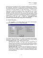
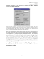
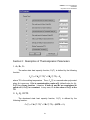
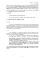
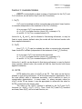
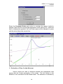
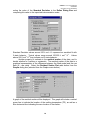
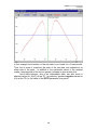
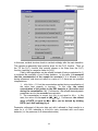
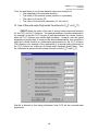
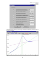
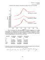
DSCFIT
©
Flexible, Rapid and Automated Analysis of Differential Scanning
Calorimetry Data
USER'S MANUAL
Version 15.3
3/25/2002
Sasha B. Grek, John K. Davis and Dr. Michael Blaber
Institute of Molecular Biophysics
Florida State University
Tallahassee, FL 32306-4380
TEL: (850) 644-5870
FAX: (850) 561-1406
[email protected]
This work was supported by a grant from the Florida Space Grant
Consortium
http://wine1.sb.fsu.edu/DSCfit/
DSCFIT © v.15.3 User's Manual
03/25/2002
http://wine1.sb.fsu.edu/DSCfit/
Table of Contents
Program Description
System Requirements and Limitations
How to Use this Manual
Section 1: General Steps in Data Analysis
I. Loading of Data
II. Initial Guess of Thermodynamic Parameters
III. The Graphs Dialog Box
IV. The Refine Dialog Box
Section 2: Description of Thermodynamic Parameters
I. A0, B0, C0
II. A1, B1, DC
III. DD
IV. TD
V. K
Section 3: Available Models
I. CN(T)
II. CD(T)
III. DCTD
IV. DDTD and TD
V. k
Section 4: Advanced Topics
I. Data Clipping
II. Evaluation of Non-2-state Behavior
III. Use of Second-order Polynomial Functions for CN(T)
or CD(T)
IV. Determination of Thermodynamic Constants at
Temperatures other than TD
V. More than One Possible Solution for Refined
Parameters
VI. Situations Where TD Does Not Exist
Section 5: Derivations
Section 6: Output of Function Data for Use in Other Programs
2
2
2
References
Referencing DSCFit in your publications
29
29
1
3
4
5
6
8
8
9
9
9
10
10
10
11
11
11
13
18
20
20
21
22
28
DSCFIT © v.15.3 User's Manual
03/25/2002
http://wine1.sb.fsu.edu/DSCfit/
Program Description
DSCFIT is designed to analyze data from differential scanning calorimetry
(DSC) experiments. It uses a statistical mechanics-based two-state model in
combination with an optimized non-linear least-squares fitting routine. The
program is designed to be flexible, rapid, and require a minimum of operator
intervention. By setting appropriate parameters, users can customize the type of
model to be used in fitting the data. DSCFIT has the unique ability to evaluate
concentration errors in DSC data, in addition to the determination of van't Hoff
and calorimetric enthalpies.
System Requirements and Limitations
DSCFIT is a Windows™ 95/98/NT based program. A graphics display of
at least 800x600 is required. A minimum of 32 MB of system memory is also
required. The disk space requirements of the program are quite modest
(currently <5 MB). As currently implemented, DSCFIT can analyze data sets with
2000, or fewer, data points. Data from both upscan and downscan experiments
can be analyzed.
Please report all bugs, etc. to:
Dr. Michael Blaber
Institute of Molecular Biophysics
Florida State University
Tallahassee, FL 32306-4380
TEL: (850) 644-5870
FAX: (850) 561-1406
[email protected]
Suggestions for improvements to DSCFIT are also welcome.
How to Use this Manual
If you are ready to analyze a data set, proceed to section 1 (General
Steps in Data Analysis). General descriptions of thermodynamic parameters are
found in Section 2, and derivations of the thermodynamics parameters are found
in Section 5. Section 3 (Available Models) and Section 4 (Advanced Topics)
provide information on the various features of the program and their application
in data analysis.
2
DSCFIT © v.15.3 User's Manual
03/25/2002
http://wine1.sb.fsu.edu/DSCfit/
Section 1: General Steps in Data Analysis
I. Loading of Data
The DSC data to be analyzed in DSCFIT should be a finalized molar heat
capacity data file. In other words, it should be a protein/buffer run that has had
the buffer/buffer run subtracted, and then been normalized for the molar
concentration of the protein (although, as discussed in the Advanced Concepts
section, DSCFIT can determine the apparent molar concentration with certain
assumptions). The data file should be a text file consisting of two columns: the
first column will contain the temperature data, and the second column will contain
the corresponding values for the molar heat capacity. These columns of data
may be separated by either a space (or spaces) or a tab character. DSCFIT will
not currently parse data delineated by other characters (e.g. commas). The
temperature can be either in °C or K, and the molar heat capacity can be in either
calorie or Joule units (DSCFIT works internally with K and Joules, however).
Load data by using either the File→Load Data menu command, or the
"Load Data" command on the menu bar. A dialog window will open enabling you
to specify the desired data file (the default file extension is *.dat). When reading
in the data file, DSCFIT will present you with a dialog box to allow conversion of
°C or calorie-based data to K and Joules:
Select the appropriate radio buttons for the units of the input data (in cases
where the temperature appears to be in °C rather than K, DSCFIT will alert the
user to the need to convert). The temperature and heat capacity units are
independent. Thus, if for some bizarre reason your raw data is in °C and Joules,
select the radio buttons for Celsius and Joules.
3
DSCFIT © v.15.3 User's Manual
03/25/2002
http://wine1.sb.fsu.edu/DSCfit/
After reading the data file, DSCFIT will report the number of successfully
imported data points, and the temperature range of the data:
Before continuing, be sure that this information is as expected for the data file in
question.
Note: Currently, DSCFIT applies the conversions of K=(273.15+°C), and
Joules=(calories/4.184) directly to the data when imported. If a mistake is made
with the units when importing the data, close the project window and read in the
data file again.
II. Initial Guess of Thermodynamic Parameters
After reading in a data file DSCFIT will automatically determine an initial
guess for the various thermodynamic parameters, and report these values in the
Parameters Dialog Box:
4
DSCFIT © v.15.3 User's Manual
03/25/2002
http://wine1.sb.fsu.edu/DSCfit/
At this point you can simply click 'OK' to accept the program's initial guesses for
the parameters. Alternatively, you can modify any of the parameters. Checking
the left-hand side box next to a parameter will constrain the parameter during
refinement to the value indicated in the right-hand side box. Leaving the lefthand side box unchecked will allow the value of the parameter to vary during
refinement to improve the agreement of the model with the data. Three
parameters, A0 (the second order term for the native state heat capacity
function), A1 (the second order term for the denatured state heat capacity), and k
(the concentration constant) are constrained (as indicated by the appropriately
checked box) to values of 0, 0, and 1, respectively. The text descriptions of
these parameters are also boxed, to indicate that refinement of these
parameters may be justified only under certain circumstances.
III. Graphs Dialog Box
After assignment of the initial values for the various thermodynamic
parameters DSCFIT will display the Graphs Dialog Box:
The Graphs Dialog Box allows you to select the appropriate thermodynamic
function(s) for viewing as a graph. The graph chosen will be actively updated
during the refinement cycle. The available functions include:
Raw Data and Fit Curves - this graph will include the raw data an can
also include the functions for the native state heat capacity function,
denatured state heat capacity function as well as the fitted function based
upon the current values of the various thermodynamic variables. This is
the default graphic representation.
Residual Scatter Plot - this graph shows the disagreement between the
fitted function and the raw data. It is useful for determining the magnitude
of the error (i.e. whether it is within the expected instrumentation noise
level) and whether the error is random, or systematic (indicating possible
non-2-state behavior).
5
DSCFIT © v.15.3 User's Manual
03/25/2002
http://wine1.sb.fsu.edu/DSCfit/
Delta Cp, Delta H, Delta G, Delta S - plots for these thermodynamic
functions.
On the left-hand side of the Graphs Dialog Box are parameters used in graphic
the various functions. The default values are to autoscale Y, and the
temperature range is the minimum and maximum of the data points.
V. Refine Dialog Box
After the appropriate graph has been selected the graph will be shown,
along with the Refine Dialog Box:
The Refine Dialog Box allows you to select the criteria for convergence of the
model fit to the experimental data. The choices include: 1) refine for a fixed
number of cycles, or 2) refine until no further improvement in the merit function is
observed over a given number of refinement cycles, or 3) refine until the
improvement in the merit function decreases to a specified value, or 4) refine
until the standard deviation of the fit decreases to a specified value. Additionally,
there is a button labeled Coefficients. Selecting this button will bring up the
Coefficients Dialog Box (where the values of the various thermodynamic
parameters can be manually entered, or the constrain check boxes may be
selected or deselected).
Clicking the button labeled 'Begin' will start the refinement of the thermodynamic
parameters (to improve the fit with the raw data). The refinement will proceed
until the selected criteria for convergence has been met. If more than 100 cycles
of refinement are performed without the convergence criteria being met, the
program will exit from refinement with an alert message.
6
DSCFIT © v.15.3 User's Manual
03/25/2002
http://wine1.sb.fsu.edu/DSCfit/
Statistical information on the refinement is available within Error Analysis
section of the Refine Dialog Box:
The information includes: 1) the value of the χ2 merit function, 2) the last value
observed for the change in the merit function, 3) the standard deviation of the fit
to the experimental data, and 4) the number of iterations that have occurred
since an improvement in the merit function was observed.
Each time the refinement routine identifies values that improve the agreement of
the model with the raw data the currently displayed graph will be updated. When
is the refinement of the thermodynamic parameters complete? As refinement
proceeds, the value for the χ2 merit function should decrease, although a target
value is difficult to know in advance. The value for ∆χ2 should also decrease,
with values typically smaller than 1 x 10-5 typical of convergence. The standard
deviation should also decrease. Target values for the standard deviation would
be related to the expected error for the instrument (e.g. on the order of 100-200 J
mol-l K-1). If the fit has converged, many cycles (i.e. >10) of refinement will occur
without an improvement in the fit.
Clicking on the Coefficients button in the Refine Dialog Box will bring up
the Coefficients Dialog Box from which the values for the refined thermodynamic
parameters can be read:
7
DSCFIT © v.15.3 User's Manual
03/25/2002
http://wine1.sb.fsu.edu/DSCfit/
Section 2: Description of Thermodynamic Parameters
I. A0, B0, C0
The native state heat capacity function, CN(T), is defined by the following
function:
CN(T) = 3*A0*(T-TD)2 + 2*B0*(T-TD) + C0
where TD is the melting temperature. Thus, CN(T) is a second-order polynomial
when A0 is non-zero. If A0 is constrained to a value of 0 (default value for A0),
CN(T) is a linear function. Likewise, if both A0 and B0 are constrained to
values of 0, CN(T) is a constant. In any case, C0 is the value of CN(T) at the
TD.
II. A1, B1, DCTD
The denatured state heat capacity function, CD(T), is defined by the
following function:
CD(T) = 3*A1*(T-TD)2 + 2*B1*(T-TD) + (DCTD + C0)
8
DSCFIT © v.15.3 User's Manual
03/25/2002
http://wine1.sb.fsu.edu/DSCfit/
where TD is the melting temperature. Thus, CD(T) is a second-order polynomial
when A1 is non-zero. If A1 is constrained to a value of 0 (default value for A1),
CD(T) is a linear function. Likewise, if both A1 and B1 are constrained to
values of 0, CD(T) is a constant. DCTD is the value of ∆Cp(T) at the TD. Since
∆Cp(T) is defined at CD(T) - CN(T), and C0 is the value of CN(T) at the TD, (DCTD
+ C0) is equal to the value of CD(T) at the TD.
III. DDTD
DDTD is defined by the following function:
∆H(T) = (A1-A0)*(T-TD)3 + (B1-B0)*(T-TD)2 + DCTD*(T-TD) + DDTD
Thus, DDTD is the value of ∆H(T) at the TD.
IV. TD
Formally, it is the temperature at which the native and denatured states
are equally populated. TD must exist. In other words, the model requires that
there be some definite temperature at which the native and denatured states are
equally populated. If the conditions are such that the native is never more than
50% populated, the analysis will fail.
V. k
The k parameter is a scalar term applied to the raw data molar heat
capacity. If it is allowed to float during refinement, and does not refine to a value
of 1.0, there are two possible interpretations:
1. ∆HvH/∆Hcal = 1.0, but the concentration applied during normalization of
the molar heat capacity is incorrect.
In this case, the actual
concentration of the protein in the DSC analysis is: (the value used
during the normalization / k). Furthermore, the refined thermodynamic
parameters are for the corrected concentration.
2. The concentration is correct, but ∆HvH is not equal to ∆Hcal. In this
case, the value of k is equal to (∆
∆HvH/∆
∆Hcal). Furthermore, the refined
value of DDTD is equal to ∆HvH. ∆Hcal can be derived by dividing
DDTD (van't Hoff enthalpy) by k.
Thus, k should only be allowed to float if other data is available to confirm
either the concentration, or the value of ∆HvH/∆Hcal (see Advanced Topics
section).
9
DSCFIT © v.15.3 User's Manual
03/25/2002
http://wine1.sb.fsu.edu/DSCfit/
Section 3: Available Models
DSCFIT is customizable to allow a variety of treatments for the CN(T) and
CD(T) functions, as well as the ∆Cp(T) and ∆H(T) functions).
I. CN(T)
CN(T) can be modeled as either a second-order polynomial, linear function
or constant (independent of the treatment of the CD(T) function):
A0 is non-zero: CN(T) is a second-order polynomial
A0 = 0: CN(T) is a linear function (slope = B0, y intercept = C0)
A0 and B0 = 0: CN(T) is a constant equal to C0
Values for A0, B0 and C0 can be allowed to float during refinement, or may be
fixed at some operator defined value (the model will find the best function with
these applied constraints).
II. CD(T)
Like CN(T), CD(T) can be modeled as either a second-order polynomial,
linear function or constant (independent of the treatment of the CN(T) function):
A1 is non-zero: CD(T) is a second-order polynomial
A1 = 0: CD(T) is a linear function (slope = B1, y intercept = C1)
A1 and B1 = 0: CD(T) is a constant equal to (DCTD + C0)
Values for A1 and B1 can be allowed to float during refinement, or may be fixed at
some operator defined value (the model will find the best function with these
applied constraints).
III. DCTD
DCTD defines the value of ∆Cp(T) at the TD. This value can be fixed or
allowed to float during refinement. Of all the thermodynamic parameters, this is
the most difficult value to determine accurately, and is sensitive to errors in
concentration determination. In some cases, i.e. where accurate values for
∆Cp(T) at the TD are known, it may be appropriate to refine with the value for
DCTD constrained to the known value.
The nature of the ∆Cp(T) function is defined by the CN(T) and CD(T)
functions (i.e. ∆Cp(T) = CD(T) - CN(T)). Thus, if both CN(T) and CD(T) functions
are linear, then ∆Cp(T) will be a linear function, etc.
10
DSCFIT © v.15.3 User's Manual
03/25/2002
http://wine1.sb.fsu.edu/DSCfit/
IV. DDTD and TD
If desired, the value of ∆H(T) at the TD can be constrained.
value of TD can be constrained.
Also, the
V. k
As discussed in the Description of Thermodynamic Parameters the k
parameter is a scalar term applied to the raw data molar heat capacity.
Investigators can use the refined value of k to gauge potential errors in
concentration and inequality of ∆HvH and ∆Hcal. If it is allowed to float during
refinement, and does not refine to a value of 1.0, there are two possible
interpretations:
1. ∆HvH/∆Hcal = 1.0, but the concentration applied during normalization of
the molar heat capacity is incorrect.
In this case, the actual
concentration of the protein in the DSC analysis is: (the value used
during the normalization / k). Furthermore, the refined thermodynamic
parameters are for the corrected concentration.
2. The concentration is correct, but ∆HvH is not equal to ∆Hcal. In this
case, the value of K is equal to (∆
∆HvH/∆
∆Hcal). Furthermore, the refined
value of DDTD is equal to ∆HvH. ∆Hcal can be derived by dividing
DDTD (van't Hoff enthalpy) by k.
Thus, k should only be allowed to float if other data is available to confirm
either the concentration, or the value of ∆HvH/∆Hcal (see Advanced Topics
section).
Section 4: Advanced Topics
I. Data Clipping
The range of data to be analyzed can be defined using both a high and
low temperature cutoff value. The first step is to identify the temperature
range(s) for exclusion. Place the mouse pointer at the appropriate position in
any of the displayed graphs and click the right mouse button to obtain the x,y
coordinates of that point:
11
DSCFIT © v.15.3 User's Manual
03/25/2002
http://wine1.sb.fsu.edu/DSCfit/
Once the specific high and low temperature cutoff values have been identified,
you can limit the data range used during refinement by selecting the
Functions→Constrain Data… options from the menu bar:
This will bring up the Constrain Data Dialog box:
12
DSCFIT © v.15.3 User's Manual
03/25/2002
http://wine1.sb.fsu.edu/DSCfit/
Select the Constrain Points radio button to constrain the region of data for
analysis, then enter the low and high temperature cutoff values (in K). When the
data is subsequently graphed, the cutoff data regions will be displayed in green
and the active data points remain blue:
II. Evaluation of Non-2-state Behavior
Various criteria are used to determine whether the experimental data
agrees with the 2-state assumption of the model. The first relates to the
deviation of the raw data from the refined model. This deviation is evaluated by
13
DSCFIT © v.15.3 User's Manual
03/25/2002
http://wine1.sb.fsu.edu/DSCfit/
noting the value of the Standard Deviation in the Refine Dialog Box and
comparing this value to the expected instrumentation noise:
Standard Deviation values around 100 J mol-1 K-1 represent an excellent fit with
2-state behavior. Typical values range around 100-500 J mol-1 K-1. Values
above 500 J mol-1 K-1 may indicate non-2-state behavior.
Another property to evaluate is the residual scatter of the data, and to
decide whether is it random or systematic. The residual scatter of the data is a
graphical representation of the difference between the fitted model and the raw
data (fit - raw data). Select the Residual Scatter Plot radio button from the
Graphs dialog box (selected from the Graphs menu button):
A graph of the residual scatter will be displayed. This graph will include a vertical
green line to indicate the location of the melting temperature (TD), as well as a
blue horizontal line indicating the zero location of the scatter:
14
DSCFIT © v.15.3 User's Manual
03/25/2002
http://wine1.sb.fsu.edu/DSCfit/
Non-random distribution of the scatter can be indicative of non-2-state behavior.
A peak, or trough, centered at the TD is one of the features of a transition that is
too broad, or too narrow, to be fit by a 2-state model:
15
DSCFIT © v.15.3 User's Manual
03/25/2002
http://wine1.sb.fsu.edu/DSCfit/
In this example the transition of the raw data is too broad for a 2-state model.
Thus, the fit tends to overshoot the peak of the raw data, and undershoot on
either side of the peak. In addition to the systematic nature of the residual
scatter, the magnitude of the error is greater (compare to prior scatter plot).
Non-2-state behavior, due to an intermediate state, can also result in
aberrant values for ∆Cp(T) at the TD. In particular, apparent negative values for
∆Cp at the TD (i.e. the value of the DCTD parameter) may result:
16
DSCFIT © v.15.3 User's Manual
03/25/2002
http://wine1.sb.fsu.edu/DSCfit/
In this case, residual structure leads to residual enthalpy after the main transition.
This causes an aberrantly large positive slope for the CD(T) function. Thus, at
the TD the CD(T) function may actually appear to be lower than the CN(T)
function (resulting in a negative value for ∆Cp).
Finally, the k parameter can be refined (instead of being constrained to 1)
to evaluate the possibility of non-2-state behavior. In this case, it is essential
that the concentration of the sample be accurate! If k is allowed to float
during refinement, and does not refine to a value of 1.0, there are two possible
interpretations:
1. ∆HvH/∆Hcal = 1.0, but the concentration applied during normalization of
the molar heat capacity is incorrect.
In this case, the actual
concentration of the protein in the DSC analysis is: (the value used
during the normalization / k). Furthermore, the refined thermodynamic
parameters are for the corrected concentration.
2. The concentration is correct, but ∆HvH is not equal to ∆Hcal. In this
case, the value of k is equal to (∆
∆HvH/∆
∆Hcal). Furthermore, the refined
value of DDTD is equal to ∆HvH. ∆Hcal can be derived by dividing
DDTD (van't Hoff enthalpy) by k.
Parameter refinement of the prior data set, with k allowed to float, results in a
value for k of 0.80, indicating a ∆HvH/∆Hcal ratio consistent with non-2-state
behavior (i.e. the presence of an intermediate state).
17
DSCFIT © v.15.3 User's Manual
03/25/2002
http://wine1.sb.fsu.edu/DSCfit/
Thus, the evaluation of non-2-state behavior relies upon analysis of:
• The magnitude of the standard deviation
• The nature of the residual scatter (random vs. systematic)
• The value of ∆Cp at the TD
• The value of the refined K parameter (i.e. ∆HvH/∆Hcal)
III. Use of Second-order Polynomial Functions for CN(T) or CD(T)
DSCFIT allows the option of the use of second-order polynomial functions
for the CN(T) and CD(T) functions. The general paradigm of protein denaturation,
for example, is that the CN(T) function is well approximated by a linear function,
while the CD(T) function may exhibit slight curvature. However, over the typical
temperature ranges used to study protein thermal denaturation, this curvature is
slight and a linear function is a reasonable approximation for the CD(T) function.
The following is an example of the application of a second-order polynomial for
the CD(T) function for a data set of human acidic fibroblast growth factor. First,
the refinement is performed with a linear function for both CN(T) and CD(T):
Now A1 is allowed to float during refinement, thus CD(T) will be a second-order
polynomial:
18
DSCFIT © v.15.3 User's Manual
03/25/2002
http://wine1.sb.fsu.edu/DSCfit/
The fitted function and CN(T) and CD(T) functions look like this (note the curve of
the CD(T) function):
19
DSCFIT © v.15.3 User's Manual
03/25/2002
http://wine1.sb.fsu.edu/DSCfit/
Although DSCFIT allows the use of second-order polynomials during the
refinement, it is up to the user to decide if the use of a second-order
polynomial is valid. The key issue is the accuracy of the baselines at
temperatures far away from the TD. The use of second-order polynomial
baselines can result in unreasonable behavior at extremes of temperature. Thus,
while second-order polynomial functions for CD(T), or CN(T), may improve
accuracy at the TD, the accuracy at other temperatures may be reduced.
IV. Determination of Thermodynamic Constants at Temperatures
other than TD
It is often important to evaluate the values for the various thermodynamic
constants at temperatures other than the TD. For example, determination of the
effects of a destabilizing, or stabilizing, mutation requires that the ∆G value for
the mutant be determined at the TD of the wild-type protein (to obtain a ∆∆G
value). The value of the various thermodynamic parameters, at any reference
temperature, can be obtained by using the Functions→Evaluate Point… menus
or the Evaluate menu button. This will bring up the Evaluate dialog box:
Input the desired reference temperature (in K) in the Temperature box, and click
the Submit button. The values for the various thermodynamic parameters at this
reference temperature will be displayed.
V. More than One Possible Solution for Refined Parameters
Two cases have been observed where alternative solutions have been
obtained during refinement. Both cases can occur when the initial guess values
are poor. This situation will typically not occur if the default initial guess values
are used, but may occur with operator selected values. The first case is a
mathematically equivalent solution, but where the sign of DDTD and DCTD
parameters are inverted. This can be demonstrated using the data set from the
20
DSCFIT © v.15.3 User's Manual
03/25/2002
http://wine1.sb.fsu.edu/DSCfit/
discussion of the previous section, inverting the sign of DDTD and DCTD, and
refining:
Note that an equivalent solution has been found for the magnitude of DDTD and
DCTD parameters, but that the signs are inverted. The fitted function will be
equivalent to the "correct" solution.
The second situation involves an apparent local minimum for the refined
parameters when the initial guesses are poor, and second order polynomials for
CN(T) and CD(T) are used. This has been observed only rarely. To avoid this
potential problem, always refine using linear baselines first, then refine with
second-order polynomial functions if desired. To confirm that the solution
is not a local minimum when using second-order polynomial functions,
perform several rounds of refinement, switching back and forth between
linear and second-order functions for CN(T) and CD(T).
VI. Situations Where TD Does Not Exist
Various definitions in the model depend upon a temperature value for TD.
Data can be analyzed under conditions where the protein is significantly
destabilized. However, the data cannot be accurately analyzed if there is no
temperature at which the native and denatured states are equally populated
(i.e. no TD).
21
DSCFIT © v.15.3 User's Manual
03/25/2002
http://wine1.sb.fsu.edu/DSCfit/
Section 5: Derivations
Native state and denatured state heat capacity functions:
∆CP(T) is:
Thus, ∆H(T) can be written as:
∆S(T) is:
and ∆G:
∆G = ∆H - (T * ∆S)
This treaTDent now allows us to describe the model function using the following
parameters:
A0, B0, C0, A1, B1, DCTD, DDTD, TD
Where A0, B0, C0 are terms for the second order polynomial describing the native state
heat capacity function, A1, B1, are the first two terms for the second order polynomial
describing the denatured state heat capacity function, DCTD is the value of ∆Cp at the
melting temperature, DDTD is the enthalpy of the system at the melting temperature,
and TD is the melting temperature.
This allows us to independently define the native and denatured state baselines
as being either second order polynomial functions, linear functions or some constant
value. It also allows us to set ∆Cp at the melting temperature (i.e. DCTD) and ∆H at the
melting temperature (i.e. DDTD) to some fixed value during parameter refinement.
Thus, we now have a very flexible model, with complete control over all critical
parameters during refinement.
The fractional component of native state as a function of ∆G is equal to:
22
DSCFIT © v.15.3 User's Manual
03/25/2002
http://wine1.sb.fsu.edu/DSCfit/
By knowing the native state heat capacity function (CN(T)), the difference heat
capacity function between the denatured and native states (∆Cp), the fractional
component of native state as a function of temperature, and the enthalpy function, the
heat capacity of the system as a function of temperature can be determined:
Note: this equation should model your raw heat capacity data
A Modification to Allow for the Determination of the van't Hoff to Calorimetric
Enthalpy, or to Determine the Error in Concentration of the Protein Sample
What happens if an inaccurate value for the protein concentration is used during
the normalization of DSC data? How does this affect the fitted thermodynamic
parameters, and how can this be evaluated in the analysis? In the following example,
the protein in the DSC experiment is determined to be 0.04mM. However, during
analysis of the data, the heat capacity is normalized to three different concentrations:
0.04mM (correct), 0.08mM and 0.02mM. The resulting endotherms look like this:
Fitting our model to this data we get the following results:
23
DSCFIT © v.15.3 User's Manual
03/25/2002
http://wine1.sb.fsu.edu/DSCfit/
The fit overshoots the data normalized to 0.02mM (suggestive of a folding
intermediate), fits reasonably well with the data normalized to 0.04mM (the "correct"
concentration) and undershoots the data normalized to 0.08mM (suggestive of a van't
Hoff enthalpy greater than the calorimetric, indicative of multimers in the native state).
The refined parameters for the above fits are as follows:
Parameter
A0
A1
B0
B1
C0
DCTD
DDTD
TD
Normalized to
0.08mM
0
0
106.399543
142.2004446
-42033.46479
3276.45386
235633.051
315.5935796
Normalized to
0.04mM
0
0
491.9808408
146.4605106
-72659.20659
1771.328293
297758.6783
316.2024851
Normalized to
0.02mM
0
0
1310.731465
12.70224628
-133991.364
3131.276108
385858.7965
316.1545567
If a scalar is introduced into the basic expression for the heat capacity function the error
in the normalization of the concentration can be corrected:
24
DSCFIT © v.15.3 User's Manual
03/25/2002
http://wine1.sb.fsu.edu/DSCfit/
Here we are dividing our model for the experimentally observed heat capacity by the
scalar term k. If the above three data sets are re-analyzed with this new model we get
the following results:
Parameter
A0
A1
B0
B1
C0
k
DCTD
DDTD
TD
Normalized to
0.08mM
0
0
305.4946027
152.5561894
-58243.45094
1.526433462
2273.729531
271551.4875
316.0675458
Normalized to
0.04mM
0
0
305.4946039
152.5561889
-58243.45113
0.7632167336
2273.729583
271551.4878
316.0675458
Normalized to
0.02mM
0
0
305.4945983
152.5561915
-58243.45016
0.3816083605
2273.729321
271551.4863
316.0675458
The parameters refine to identical values except for the k parameter, which
reflects the concentration error in the normalization. Why is the value for k not equal to
1.0 for the data set normalized to 0.04mM? One possibility is that our sample is not
actually at 0.04mM (but is actually 0.052mM). Alternatively, the protein may not exhibit
two-state denaturation, and thus, the van't Hoff and calorimetric enthalpies may not be
equal (i.e. ∆HvH/∆Hcal does not equal 1.0). How does a non-equality of the van't Hoff
and calorimetric enthalpies affect the analysis?
Here is a fit to a simulated DSC run with the following parameters:
25
DSCFIT © v.15.3 User's Manual
03/25/2002
http://wine1.sb.fsu.edu/DSCfit/
TD = 323.15 K, Hcal = 167.4 kJ/mol, HvH = 334.9 kJ/mol, (∆HvH/∆Hcal = 2.0), (∆Cp
= 0, slopes for baselines = 0)
The fit undershoots the peak, indicating a situation where the ∆HvH/∆Hcal is
greater than 1.0 (with possible multimers in the native state). In any case, a two-state
model does not fit the data. The parameters of the fit are:
Parameter
A0
A1
B0
B1
C0
DCTD
DDTD
TD
0
0
0
0
0
0
220899.7025
323.223306
What happens to the fit if we include the same scalar, k, as before? Here are the
results of the fit:
26
DSCFIT © v.15.3 User's Manual
03/25/2002
http://wine1.sb.fsu.edu/DSCfit/
Parameter
A0
A1
B0
B1
C0
k
DCTD
DDTD
TD
0
0
0
0
0
1.99901503
0
334715.0703
323.1500011
In this case, DDTD agrees with the expected value for the van't Hoff enthalpy
(334.9 kJ/mol). The value for the parameter k agrees with the ratio of ∆HvH/∆Hcal (2.0).
∆Hcal can now be derived by dividing DDTD (van't Hoff enthalpy) by k (∆HvH/∆Hcal) ,
yielding 167.4 kJ/mol.
Conclusions:
•
•
Errors in concentration or situations where the van't Hoff enthalpy do not agree
with the calorimetric enthalpy can result in a similar situation - errors in enthalpy
and deviation of the fit with a 2-state model
Introduction of a scalar (k) in the model can correctly adjust the model for two
situations: 1) errors in concentration (assuming van't Hoff and calorimetric
27
DSCFIT © v.15.3 User's Manual
03/25/2002
http://wine1.sb.fsu.edu/DSCfit/
enthalpies are equal), and 2) determination of the van't Hoff to calorimetric
enthalpy ratio (assuming concentration is correct).
Section 6: Output of Function Data for Use in Other Programs
Data associated with relevant thermodynamic functions can be output for use in
other programs. This is particularly useful for presentation quality graphics. To output
function data, choose the Functions→
→Export File command:
You will be given the option of adding comments to the top of the output file. You can
output the file as either a text or .csv file (which can be read directly into popular
spreadsheet programs). The output of a typical .csv file will look like this:
Ao
Bo
Co
A1
B1
DCTD
DDTD
TD
k
0
99.9690
-121530
0
435.449
-6497.17
-257266
312.5667
1
C(T)
CpN(T)
CpD(T)
DCp(T)
DH(T)
DS(T)
Temperature Raw Data
287.276
-149246
-148519.8
Residual
Scatter
-726.19735
DG(T)
Fn(T)
-126587
-150053
-23466
121631
451.06386
287.55
-148989
-148426.5
-562.50016
-126532
-149814
-23282
115227
428.78033
-8068.47 0.033087
287.823
-148713
-148316.5
-396.49734
-126477
-149577
-23099
108896
406.77338
-8182.52 0.031694
288.097
-148446
-148191.07 -254.92639
-126422
-149338
-22915
102592
384.8814
-8290.97
288.373
-148220
-148051.33 -168.67178
-126367
-149098
-22730
96293
363.02736
-8394.17 0.029279
-7947.93 0.034633
0.03043
This output data includes the input raw data, fitted Cp(T) function, residual scatter,
native and denatured state baselines, ∆Cp(T), ∆H(T), ∆S(T), ∆G(T) and FN(T) (fraction
native state) functions.
28
DSCFIT © v.15.3 User's Manual
03/25/2002
http://wine1.sb.fsu.edu/DSCfit/
References
Kidokoro, S.-I. and A. Wada (1987). "Determination of thermodynamic functions
from scanning calorimetry data." Biopolymers 26: 213-229
Freire, E. and Biltonen, R.L. (1978). "Statistical mechanical deconvolution of
thermal transitions in macromolecules. I. Theory and application to
homogeneous systems." Biopolymers 17:463-479
Referencing DSCFit in your publications
Details of the DSCFit program have been published in the following:
An Efficient, Flexible-Model Program for the Analysis of Differential Scanning
Calorimetry Data , Grek, S., Davis, J. and Blaber, M. Protein and Peptide Letters
6, 429-436 (2001)
29