Download Table Of Contents

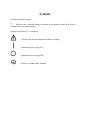
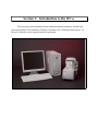
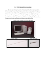
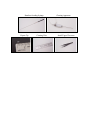
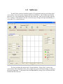
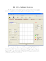
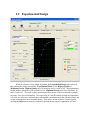
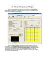
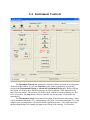
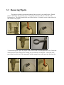
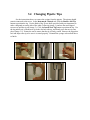
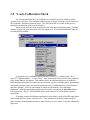
Table Of Contents
General................................................................................................................................1
How To Use This Manual................................................................................................1
How to Get Help from MicroCal.....................................................................................2
MicroCal, LLC Contact Information......................................................................................................3
Symbols............................................................................................................................4
Operational Safety...........................................................................................................5
Instrument Specifications.................................................................................................6
Performance Specifications.....................................................................................................................6
Physical Specifications...........................................................................................................................6
Electrical Specifications..........................................................................................................................6
Atmospheric Specifications....................................................................................................................6
Section 1: Introduction to the iTC200............................................................................8
1.1 The Basics of ITC....................................................................................................9
1.2 Parts and Accessories.............................................................................................10
1.3 Software.................................................................................................................12
Optional Origin.....................................................................................................................................13
1.4 Basics of Performing a Run...................................................................................14
Loading the Syringe..............................................................................................................................14
Loading the Cell....................................................................................................................................14
1.5 Tutorial Experiments.............................................................................................16
Water/Water Tutorial...........................................................................................................................16
CaCl/EDTA Tutorial.............................................................................................................................17
Section 2: iTC200 Software and Origin.......................................................................18
2.1 iTC200 Software Overview...................................................................................19
2.2 Experimental Design..............................................................................................21
2.3 Advanced Experimental Design............................................................................23
Calculating Concentrations...................................................................................................................25
2.4 Instrument Controls...............................................................................................27
States of Operation................................................................................................................................28
2.5 Real Time Plot.......................................................................................................30
2.6 Setup......................................................................................................................31
2.7 Menu Options.........................................................................................................33
2.8 Origin Real-Time Display......................................................................................35
2.9 Origin Data Analysis Tutorial ...............................................................................37
Section 3: Instrument Maintenance.............................................................................38
3.1 Cleaning the Cells and Syringe..............................................................................39
Cell Cleaning.........................................................................................................................................39
Syringe Cleaning...................................................................................................................................41
3.2
3.3
3.4
3.5
3.6
Changing Injection Syringes..................................................................................43
Removing Pipette...................................................................................................45
Changing Pipette Tips............................................................................................46
Y-axis Calibration Check.......................................................................................47
Temperature Calibration Check.............................................................................49
General
How To Use This Manual
This manual describes the iTC200 operation, software and maintenance. Section 1
contains general descriptions of the system, its parts and tools, the software, how to perform a
run, and the tutorials. These tutorials are recommended to every new user, to acquaint them with
the software and methods and to ensure optimal performance from the instrument. Section 2
describes the software in greater detail. Section 3 describes routine maintenance that users may
need to perform, from basic cleaning, to periodic calibration checks, to removal and replacement
of parts.
How to Get Help from MicroCal
The service department at MicroCal, LLC is available to help you during normal business
hours, Monday through Friday from 8:00 AM to 5:00 PM (EST). The European office is
available during normal business hours, Monday through Friday from 9:00 AM to 5:00 PM
(GMT).
Service personnel may be contacted by e-mail, phone or fax, with preference being phone
or e-mail. When e-mailing MicroCal for technical assistance, if possible, please attach a recent
data file(s) (*.itc, raw ITC data file) that demonstrates the problem. Also, please include all
details that may be relevant to the problem. For instances where the problem or question relates
to post run data analysis, it is best to attach both the raw data file (*.itc) and the Origin project
file (*.opj) generated during data analysis.
There are two general categories of troubleshooting for the iTC200 and its operation. The
most extreme category is when a system is not working at all. Problems that prevent users from
operating the iTC200 require immediate consultation with a MicroCal technician. Customers
should not attempt to repair the iTC200 hardware or software unless instructed to do so by a
MicroCal service representative.
The second, and less extreme general category of a problem is when an iTC200 instrument
is functioning, but is not operating within its normal performance specifications. Large baseline
drifting, non-repeatable control peaks (water/water) and/or an increase in short term noise level
are examples of performance problems. These problems may be corrected by the operator in
most cases. For these types of performance issues it is recommended that customers carry out
the following minimum diagnostic steps prior to contacting MicroCal for service:
1. Thoroughly clean the cells. Do not assume they are clean; build-up or unexpected
sample residue will cause problems. As a minimum, use the provided Cell Cleaning
Apparatus to pass at least 50 ml of 10-15% detergent in water solution, followed by 50
ml of water, through the sample cell. Discretion may call for a more rigorous cleaning
procedure.
2. Using a clean Hamilton syringe, refill both the reference and sample cells with filtered
degassed water. Thoroughly clean the titration syringe or use a different syringe. Load
the syringe with water.
3. Go to the Setup window within the iTC200 software and activate the extended data mode.
While the software is in the extended data mode, the ITC data files will contain all
available information produced by the iTC200. This additional information will often help
the MicroCal technician diagnose problems.
4. Carry out a minimum of 20, 1μL injections of water into water.
If, after completion of the 4 steps listed above, the ITC performance is not corrected, please
contact the MicroCal service department for help. The water run, in extended data mode, should
be provided to the MicroCal service technician for evaluation. Following the evaluation, a
representative from the service department will contact you with comments and
recommendations.
MicroCal, LLC Contact Information:
Primary Contact Phone:
Toll Free Phone Number:
Fax:
European Office:
European Fax:
Web Site:
Service E-mail:
Customer Service E-mail:
413-586-7720
800-633-3115
413-586-0149
44 1908 576330
44 1908 576339
www.microcal.com
[email protected]
[email protected]
Please forward corrections or suggestions concerning this manual to [email protected]
Origin® is a registered trademark of Origin Lab, Northampton, MA
MicroCal™ is a registered trademark of MicroCal, LLC, Northampton, MA
Windows™ is a registered trademark of Microsoft Corporation
Symbols
Symbols used in this manual:
!
Warns the user of possible damage to the unit, draws attention to the risk of injury or
contains safety notes and warnings.
Symbols used on the iTC200 instrument:
Caution: Read the instruction manual before operating
Instrument (power supply) ON
Instrument (power supply) OFF
Protective Ground (earth) Terminal
Operational Safety
The points below are intended to enhance your safety awareness and to draw your
attention to risks which only you, the operator, can prevent. While MicroCal works to ensure
that the instrument is designed and tested to be as safe as possible, proper handling is also
critical. The operators should be responsible people trained in basic laboratory protocol, and
they should be familiar with the possible hazards before operating this instrument. All
instrument modifications should be performed only by personnel trained by MicroCal.
Equipment damage, personal injury or even death may result if this equipment is operated,
altered or maintained by untrained personnel or in an irresponsible or improper manner.
!
Provide proper electrical power to the instrument. This should be 110 – 240 Volt,
50/60 Hertz alternating current, with a Ground Fault Circuit Interrupter (GFCI). Most power
strips, including those provided by MicroCal, contain a GFCI. All power plugs and cords should
be 3-prong, grounded cables or outlets.
!
Replace fuses ONLY with 3.15 Amp 250 Volt Time Delay Fuses. Several spare fuses
are provided with the original shipment.
!
Repairs, alterations or modifications must only be carried out by specialist
personnel, or with explicit directions from a MicroCal technician. Removal or
modification of any cover or component could result in an unsafe or easily damaged
instrument. The MicroCal service department will be happy to answer any questions and
provide parts and service when necessary.
!
A solution can become an electrical conductor when in contact with electricity. Use
caution when using solutions near the instrument. If any liquid is spilled on or around the
instrument, unplug the instrument immediately and wipe it up. Be careful not to overflow the
small reservoirs around the cell access tubes. If there is any possibility that liquid may have
leaked into the instrument case, contact MicroCal immediately. Do not plug the instrument into
any electrical outlet until the problem is resolved.
!
The operator should always follow proper laboratory procedures in handling and
disposing of volatile or hazardous solutions.
!
All solutions in the cells must be cooled down below 40 ºC before removal. Any
higher temperature may cause the syringe to break, and will increase the dangers of most
hazardous solutions.
!
Never allow liquid in the cells to freeze. The expansion of the liquid can distort the
cells and rupture the most critical sensor, causing irreparable damage.
!
The iTC200 instrument should always be moved in its normal operating orientation.
Other orientations will subject delicate sensors inside the instrument to stress.
!
The iTC200 cells are constructed out of Hastalloy. Strong acids should be avoided.
Please refer to the accompanying material analysis booklet for further information.
!
This instrument is not designed to the Medical Devices Directive 93/42/EEC and should
not be used for medical purposes and/or in the diagnosis of patients.
Instrument Specifications
Performance Specifications:
Operating Temperature Range: 2 - 80°C
Response Time: 10 seconds
Cell Design: 200µL, coin-shaped
Titration Syringe: 40µL
Maximum Usable Volume: 35µL
Smallest Injection Size: 0.1µL
Stirring Rate: 300 – 1500 RPM
Physical Specifications:
Cell Material: Hastelloy® Alloy C-276
Dimensions:
Calorimeter: 6½ x 13 x 10½“
Controller: 15½ x 16½ x7½”
Monitor: 17½ x 16 x 5½”
Weight (pounds)
Calorimeter: 16
Controller: 20
Monitor: 9.5
Electrical Specifications:
All electrical specifications are for the calorimeter only.
Electrical Ratings:
Voltage: 110 - 240 Volts
Frequency: 50 / 60 Hz
Power: 70 Watts
Fuses (2): 3.15A, 250V, Time Delay
Output: Secondary/Data Connection Only
Protective Earth Terminals: Internal/external marked
Mode of Operation: Continuous
Classification: Class I
Atmospheric Specifications:
Operating:
Temperature: 10 - 40 °C
Humidity: 0 - 70% RH non-condensing
Atmospheric Pressure: 700 – 1060 HPa
Storage (no liquid in cells):
Temperature: -40 - 70°C (no liquid in cells)
Humidity: 10 - 90%
Atmospheric Pressure: 500 – 1060 HPa
Section 1: Introduction to the iTC200
This section provides information about isothermal titration calorimetry and the basic
parts and operation of the Isothermal Titration Calorimeter (ITC) instrument and software. At
the end, it includes several suggested tutorial experiments.
1.1 The Basics of ITC
The iTC200 (Isothermal Titration Calorimeter, 200μL cell) unit directly measures heat
evolved or absorbed in liquid samples as a result of mixing precise amounts of reactants. A
spinning syringe is utilized for injecting and mixing of reactants. Spin rates are user selectable;
the usual range is 500 to 1000 RPM. The normal temperature operating range is 1°C to 80°C.
Wetted cell surfaces are Tantalum or Hastalloy, which are resistant to most solutions, however,
strong acids and strong bases should be avoided.
Sample and reference cells are accessible for filling and cleaning through the top of the
unit. The sample cell is on the left as one faces the front of the unit. A pair of identical coin
shaped cells is enclosed within two shields; the inner shield is referred to as the jacket. Access
stems travel from the top exterior of the instrument to the cells. Both the coin shaped cells and
the access stems are completely filled with liquid during operation. This requires approximately
250 μL per cell even though the working volume of the cell is only 200 μL.
Temperature differences between the reference cell and the sample cell are measured,
calibrated to power units and displayed to the user as well as saved to disk. The data channel is
referred to as the DP signal, or the differential power between the reference cell and the sample
cell. This signal is sometimes thought of as the “feedback” power used to maintain temperature
equilibrium. Calibration of this signal is obtained electrically by administering a known quantity
of power through a resistive heater element located on the cell.
In a typical experiment, the syringe containing a ligand is titrated (injected) into the cell
containing a solution of macromolecule. An injection which results in the evolution of heat
(exothermic) within the sample cell causes a negative change in the DP power, since the heat
evolved chemically provides heat that the DP feedback is no longer required to provide. The
opposite is true for endothermic reactions. Since the DP has units of power, the time integral of
the peak yields a measurement of thermal energy, dH. This heat is released or absorbed in direct
proportion to the amount of binding that occurs. When the macromolecule in the cell becomes
saturated with added ligand, the heat signal diminishes until only the background heat of dilution
is observed.
With the iTC200 system the entire experiment takes place under computer control. The
user inputs the experimental parameters (temperature, number of injections, injection volumes)
and the computer carries out the experiment. Origin software is then used to analyze the ITC
data using fitting models to calculate reaction stoichiometry (n), binding constant (Ka), enthalpy
(ΔH) and entropy (ΔS).
1.2 Parts and Accessories
The main parts of the system are the cell unit and controller. The tower, on top of the
iTC200 cell unit, guides the motion of the pipette, which holds the titration syringe. The pipette
has three positions; cleaning, loading, and run positions It may also be placed in a neutral or rest
position inbetween the other positions. A glass 0.5 mL Hamilton loading syringe is used to fill
and rinse the sample and reference cells. The cell cleaning apparatus, consisting of a small
plastic barrel and soft tubing, is used to run liquid through the sample cell for rinsing and basic
cleaning. A screw and ferrule fitting attaches to the pipette for rinsing and filling. Also, a thin
piece of wire is provided for vigorous cleaning of the titration syringe tip. Several other tools are
provided for removal and replacement of the titration syringe and pipette tip.
Complete System: Controller; Cell, Tower, and Pipette
Titration Syringe
Soft-Grip Tweezers
Hamilton Loading Syringe
Pipette Tip
Cleaning Wire
Cleaning Apparatus
Small-Tipped Tweezers
1.3 Software
In order for the system to initialize properly, all components must be powered up in the
correct order. First, boot up the computer and log in to Windows. Once Windows has started,
power the iTC200 by operating the switch at the rear of the unit. After several seconds, open the
iTC200 software. If the option is selected, a real-time copy of Origin will open automatically, as
well as the iTC200 control software.
The line just below the menus reads “System Initiation – Please Wait”, which is the
current status of the instrument. After a few seconds, the system will begin heating or cooling to
the preset temperature. To the right of that, the Time Left box, during a run, will show the time
left until the end of the run.
When the software is first started, the Experimental Design tab is selected; this contains
the simple run controls. Experimental Mode can be Highest Quality or Minimum Protein.
The expected n, Kd, and Delta H and the desired run temperature will allow the software to
calculate the recommended concentrations for the cell and syringe, and set the run parameters.
The Advanced Experimental Design tab contains more direct controls for the more advanced
user. This tab should be very familiar to users of the VP line of instruments. The Instrument
Controls tab allows the user to name the output files, choose post-run analysis options, and start
and stop the run. The Real Time Plot tab shows the data currently being generated. The Setup
tab contains various options and preferences.
Optional Origin:
The copy of Origin that is opened by iTC200 software, if desired, is for real-time data
display. For analysis, the user should open a separate copy. At the top of the graph screen, the
current status of the instrument is shown. Below that, the file name that the software is currently
saving to is displayed. The graph displays DP in μCal/sec verses time in seconds. The Main
Display box in the upper left corner shows the temperature of the cells, current DP, and DT. The
lower left corner contains the graph view options: Rescale To Show All resizes the window to fit
whatever data is currently displayed in it, Auto-View 1 and Auto-View 2 set the window to a
certain scale, with the latest data point centered vertically, and Saved View 1 and Saved View 2
set the Y-axis to a specific range. All four of these views can be edited through the Edit ranges
button.
1.4 Basics of Performing a Run
In order to perform a basic ITC titration experiment, the user must load the sample cell
and the syringe, enter the desired parameters into the control software, and click Start. The
reference cell should be filled with water or buffer, and may be left for several days.
Loading the Syringe:
To load the titration syringe, place a microcentrifuge tube in the tube holder. Be sure to
push the tube to the bottom of the holder with the lid fitting into the slot provided (see image
below). Be careful not to leave any part of the tube in the path of the syringe needle to prevent
damage.
Disconnect the filling tube from the ThermoVac unit and connect the threaded end to the
pipette fill port if necessary (it should still be in place after cleaning and drying of the syringe).
Insert the tip of the 1 mL plastic syringe into the end of the filling tubing. In the software, under
the Instrument Controls tab, click the Open Port button to make sure that the pipette fill port is
open. Slide the pipette up, across, and down into the middle slot, so that the tip of the syringe
rests in the microcentrifuge tube. Gently pull up on the plunger, until the sample has filled the
titration syringe and is just overflowing into the tubing.
Click the Close Port button to close the fill port. Pull the plunger up approximately
another 0.1mL to remove the excess liquid in the tubing, and disconnect the tubing from the fill
port. Click the Purge/Refill button 2-3 times to move the pipette tip down and back up again,
dislodging any air bubbles on the glass sides of the syringe.
Loading the Cell:
To load the sample cell, gently insert the glass Hamilton syringe into the (left) sample
cell until it touches the bottom. Pull up on the plunger until bubbles are being pulled from the
cell, and there is no more liquid. Remove and empty the syringe. Clean the syringe if necessary.
Pull approximately 300 µL of sample into the syringe, and tap the syringe glass so that all air is
at the top volume of the syringe. Do not allow air to be put into the cells. After removing the
bubbles, insert the syringe into the cell and gently touch the bottom of the cell with the tip of the
syringe needle. Raise the needle tip about 1 mm off the bottom of the cell, and hold it there until
finished filling. Do not raise the syringe during the filling process. Slowly inject solution into
the cell until it spills out the top of the cell stem. Finish the filling with several small abrupt
spurts of solution to dislodge any bubbles in the cells. Finally, lift the tip of the syringe to the
cell port (just below the visible portion of the cell port) and find the ledge that is formed where
the cell stem meets the cell port. Place the syringe on the ledge at the top of the metal cell stem
and remove the excess solution. If the reference cell needs refilling, follow the same procedure
as for the sample cell.
If there is a saved run file for the current experiment, load the run parameters by clicking
the Load Run File button at the top left of the Advanced Experimental Design tab in the iTC200
software and select the run file. There are standard run files for most of the tutorial experiments.
If no run file exists, enter parameters in the appropriate boxes in the Experimental Design tab
(see sections 1.3 and 2.2 for more information). Once the parameters have been entered, click
the Start button at the upper left corner of the Instrument Controls tab of the control software.
Be sure to insert the syringe in to the sample cell before starting the experiment. The instrument
will seek experimental temperature, equilibrate to that temperature, start the titration syringe
stirring, wait until the DP signal is steady, and then start performing injections. The raw data
will appear in the Real Time Plot tab.
Once a run has finished, the syringe and sample cell should be cleaned as soon as
possible. See Section 3.1.
1.5 Tutorial Experiments
The next two tutorial experiments are recommended for every new user before beginning
analysis of their own samples. They are designed to provide standard results, which check that
the instrument is working well and the user is comfortable with the procedures, before risking
precious sample.
Water/Water Tutorial:
The first tutorial involves titrating water into water.
1. Fill both cells with distilled water at ambient temperature, fill the titration syringe, and insert
the syringe into the sample cell.
2. Click on the Load Run File button in the Advanced Experimental Design tab, choose
“WATER.INJ”, and click Open. Name the run and click Start. The instrument will seek
the run temperature, equilibrate the system, and begin making injections. Each peak should
be small, with all the peaks approximately the same shape.
3. Once the run has finished and the instrument is thermostatting again, open the ITC
Calibrations project to analyze the data. It is located in the Origin directory, at
C:\Origin70\ITCCalibrations.OPJ.
4. Click on the Water/Water Report button. A window will pop up asking which files to
analyze; select the file you just generated, click Add Files, and click OK.
5. Origin will analyze the data for several seconds. Once it has finished, it will ask you to save
the results. Give the file a unique name. There should be a graph, with the water DP data,
and a textbox. Zoom in using the magnifying glass over a plus sign icon on the top toolbar,
so that you can read the textbox. To zoom in and read the text, select the magnifying glass
over a plus sign icon on the top toolbar and click on the textbox.
Water-Water Report
VPITC11.06.834
12/5/2006 08:42:23
Raw DP Data
10uL injections
Water-Water Specifications:
Mean Energy/Injection less than 1.5 uCal
SD less than 0.15 uCal
Baseline Offsets Have Been Manipulated!
Wws1a, Mean Energy/Injection=-0.34863uCal, SD=0.08232 uCal
Results Within Specifications
Line 2 of the script is the instrument serial number, line 3 is the date and time that the report was
generated, line 5 is the injection size, and lines 7 and 8 are instrument specifications. Origin
manipulates the offsets so that multiple water runs can be displayed without overlapping. Line
10 gives the data file name and the mean and standard deviation of the energy per injection. The
last line will say “Results Within Specifications” or “Results Outside of Specifications”. If the
results are not within specifications, you may want to run the tutorial again.
CaCl2/EDTA Tutorial:
This tutorial uses the standard sample kits provided with the instrument when it is shipped. Kits
can also be obtained from MicroCal at any time.
1. Load the titration syringe with CaCl2. The sample cell must be rinsed with EDTA in order to
obtain an accurate fitted value for stoichiometry. Fill the sample cell with EDTA and allow
the solution to remain in the cell. After 5 minutes, remove the EDTA solution from the cell.
Load a fresh volume of EDTA in to the sample cell.
2. Set the run parameters. A set of parameters is provided with the sample.
3. Name the file and click Start to begin the experiment.
4. Once all injections have been completed, clean and dry the syringe. Use the cleaning
apparatus to clean the sample cell. See section 2.9, “Origin Data Analysis Tutorial” for
analysis of the results.
NOTE – Detailed instructions concerning sample loading and data collection using the standard
CaCl2 / EDTA kit are provided with each kit.
Section 2: iTC200 Software and Origin
This section details the features of the iTC200 software. This software provides the user
an interface to control the iTC200 instrument and perform an experiment. An optional copy of
Origin can be used for plotting the data received from the iTC200 instrument. A separate copy of
Origin (Origin for ITC) is used for analyzing data.
2.1 iTC200 Software Overview
The iTC200 software contains drop down menus, a status bar, and several tabs. The drop
down menus control global system functions. The status bar displays the current status of the
instrument. Each tab contains controls for different areas of instrument control.
The status bar just below the menus reads “Thermostatting ITC @ 30°C”, which is the
current status of the instrument. When the system first loads, this bar will read “System
Initiation – Please Wait”. After a few seconds, the system will begin heating or cooling to the
preset temperature. Once the instrument reaches the set temperature, it will thermostat at that
temperature. To the right of the status bar, the Time Left box. During an experiment this box
will show the time left until the end of the run.
When the software is first started, by default, the Experimental Design tab is selected;
this contains the simple run controls. These let the user make a guess at N, Kd, and Delta H, and
have the software automatically design the experiment. The Advanced Experimental Design
tab contains more direct controls for the more advanced user. This tab should be familiar to
users of the VP line of instruments. The Instrument Controls tab allows the user to name the
output files, choose post-run analysis options, and start and stop the run. The Real Time Plot
tab shows the data currently being generated. The Setup tab contains various options and
preferences.
2.2 Experimental Design
When the software is first started, by default, the Experimental Design tab is selected;
this contains the simple run controls. Experimental Mode can be Highest Quality or
Minimum Protein. Highest Quality uses 20 injections and a c-value of 100. These parameters
should produce data that is clear and easier to fit. Minimum Protein uses fewer injections, 10,
and a c-value of 5. The result of these parameters will be the use of the least amount of sample
necessary for a successful titration. The expected n, Kd, and ∆H and the desired run temperature
will allow the software to calculate the recommended concentrations for the cell and syringe, and
set the run parameters based on mode chosen. If the user is unsure of the Kd for their system,
clicking the Help button causes the software to prompt for the type of compound in cell and
syringe. It will then make a guess as to the Kd. The user will still be required to choose values
for ∆H and n.
Click the Update Experimental Curve button to calculate the results. The simulation
window will update with a rough graph, and the Results column at the right of the screen will
have values for the cell and syringe concentrations. The calculated C value is listed below; its
background is color-coded. This value is equal to 5 in Minimum Protein mode, 100 in Highest
Quality mode, and will vary if the user chooses to change cell concentration manually. The cvalue predicts the shape or sigmoidicity of the curve. Optimal values for C are between 5 and
500 (green); values between 1 and 5, and 500 and 1000 should work but may not give the best
result (yellow). C values less than 1 or greater than 1000 will probably not yield usable data
(red). The user may adjust the two experimental concentrations by using the change buttons
beside each concentration box.
Any warnings, such as heats too high for the instrument to measure, will appear in the
status bar near the top of the screen. It is highly recommended that the users look carefully at the
projected curve and make sure that the shape and rough values are reasonable before proceeding.
A pair of options at the bottom of this tab allows users to work in Kd or Ka, and to choose
whether to view the simulation plot using raw heat per injection (DH) or the heat normalized to
the molar ratio (NDH).
2.3 Advanced Experimental Design
The advanced experimental design tab may be used in addition to the Experimental
Design tab for operating the iTC200 instrument. Below is a description and suggested values for
each of the run parameters displayed in this tab.
The top bar in this tab contains several buttons for opening, saving, and viewing run
parameter files. The Load Run File button will display the file open dialog box, in which the
user can select a file to load into the Advanced Experimental Design tab. Run parameters may
be loaded from one of two types of files: a previous experiment’s data file (*.itc) (the run
parameters are extracted from the data file header), or a setup file (*.inj) which was previously
saved using the Save Run File button.
Save Run File displays the file save dialog box which allows saving of the currently
displayed run parameters. Once the parameters have been saved, they may be reloaded and
reused in the future by selecting Load Run File as described above.
Display Run Parameters displays the current run parameters for the run in progress.
This button is available only when the iTC200 is in a non-idle state.
Update Run Parameters updates the current run parameters for the run in progress.
When the ITC is in a non-idle state, this button must be clicked for the run parameter changes to
take effect. This button is available only when the iTC200 is in a non-idle state. Note: Only run
parameters that have not yet been applied on the run in progress may be updated; all others will
be ignored (i.e. after the stirring has commenced for an experiment, changes to the experimental
stir speed will be ignored).
The Total # Injections (500 is the maximum) sets the number of injections for the
titration (ITC) experiment. The multiple-injection method requires a minimum of 10-15
injections. There are no negative consequences (except the time spent) to titrating past the point
where all sites are saturated, and these last few injections can be used for control heat
information. The single injection method uses one single longer injection.
The Cell Temperature box is used to set the desired run temperature for the experiment.
Most runs are performed between 25°C (room temperature) and 37°C (human body
temperature); although the instrument’s operating range is 2°C to 80°C.
Throughout an ITC experiment, a small constant amount of power (equal to the
Reference Power entered) is continuously supplied to the offset heater of the reference cell.
This causes the DP feedback system to become positive to supply compensating power to the
sample cell that will equilibrate the temperatures. During an experiment the DP baseline will
equilibrate near the value entered in the Reference Power box. The reference power setting is
often referred to as the baseline setting. The best choice for the reference power setting will be
determined by the anticipated size and direction of the titration peaks. Large exotherms will
require a large reference power setting (ca. 5 µCal/sec.) and large endotherms will require a very
small reference power setting (ca. 0.5 µCal/sec.). When working with an unknown sample, a
reference power of 2-3 µCal/sec is best.
The Initial Delay refers to the time, in seconds, after the instrument has started a run and
before the first injection. The standard parameter is 60 seconds; this is necessary to establish a
baseline prior to the first injection.
The Syringe Concentration and Cell Concentration boxes are a place to enter the
experimental concentrations. The Experimental Design tab will make suggestions of the proper
concentrations if desired (see section 2.2), or refer to “Calculating Concentrations” later in this
section for more information. If the Experimental Design tab was used, these values will
already be filled in. These concentration values are stored in the data file header and used for
ITC data analysis. These values are used only during data analysis and an entry is not required
to perform an experiment.
Select the desired stirring rate from the drop down list (1000 RPM is recommended for
most ITC experiments). If the solution in the sample cell contains suspended particles (e.g.
agarose beads), then faster stirring may be necessary.
In the Feedback Mode/Gain section, the three available modes are none, low or high
(High is recommended for most ITC experiments). The feedback modes can be described as
active (low or high) or passive (none). High gain will provide the fastest response time, while
passive mode (none) will provide the highest sensitivity. Almost all ITC reactions will require
using the high gain feedback mode. Monitoring of long, slow thermal process in the iTC200 (i.e.
kinetics, metabolic rates) might benefit from using the passive or low gain feedback modes.
The Data File Comments box allows the user to enter comments about the experiment to
be saved in the header of the data file for future reference.
The simulation plot in this window is generated from the Experimental Design tab.
Clicking Update Experimental Curve pulls the information from that tab to the current one. In
addition, the user may enter the Kd and dH here and change the plot from this tab.
The Injection Parameters group allows the user to define the volume, duration, spacing
between injections, and the filter period for each injection. At the bottom of this group is a
summary table that lists these parameters, ordered by injection number. The user may select an
injection to edit by clicking on a row to highlight it; the parameters for this injection can be
entered into the text boxes (see below). Then, depending on the Edit Mode selected, the user
may edit the text boxes to effect all injections (All Same), only the currently highlighted
injection (Unique) or the currently highlighted injection and all the following injections (Apply
To Rest).
In the Volume box, the user may enter the volume of titrant (in μL), to be injected from
the pipette into the sample cell for the selected injection(s).
In the Duration (sec.) box, the user may enter the time, in seconds, that the instrument
will take to inject the titrant into the sample cell. The iTC200 software will generally default this
value to be twice the number entered in the Volume text box. For Single Injection Method
(SIM) experiments, the standard duration is ten times the volume.
In the Spacing (sec.) box, the user may enter the time, in seconds, between the beginning
of the selected injection and the beginning of the next injection (or end of the run). This spacing
must allow enough time between the injections to allow the DT signal to return to the baseline
after an injection peak deflection. Typical values for this parameter range from 90-180 seconds,
depending on the size of the peak and the kinetics of the reaction. For Single Injection Method,
the spacing should be 90 - 180 seconds greater than the duration (i.e. volume = 20 μl, duration =
200 seconds, spacing = 300 seconds).
The Filter Period (sec.) is the time period (in seconds) in which the data channel
conversions are averaged to produce a single data point for plotting and saving.
For fast reactions, a filter period of 5 seconds is sufficient to obtain enough data points for
representation of the peak for accurate integration of the area. For monitoring of very long, slow
thermal processes, the filter period may be increased accordingly to avoid accumulation of
excess data points. Although there may be a practical limit for a data set size, only available disk
space would limit the number of data points that the iTC200 software is able to collect and save.
Calculating Concentrations:
The easiest way to determine a good starting concentration for a system is to use the
Experimental Design tab of the iTC200 software (see section 2.2). This section provides an
alternative method for the slightly more advanced user.
To approximate the sample concentration needed in the sample cell, estimate the Kd for
the system and multiply by 10. With very tight binders, the cell concentration should be on the
low side of this value; for weak binders, the concentration should be on the high side of this
value. Multiply the cell concentration by n and by 10 - 15 for the syringe concentration. Again,
for very tight binders, the concentration should be on the low side and for weak binders this
value should be on the high side. The minimum and maximum concentrations that are
commonly used in the iTC200 are 3µM to 500µM.
These are "rules of thumb" and not absolute. However, if Kd and n are unknown, a best
guess should provide enough data to fine-tune the parameters. An analysis of the data from the
run will show the average peak size, approximate n, and a better estimate of Kd. Either the
concentrations or the injection volumes should be adjusted so that the large initial peaks are ~1 4 µCal/second in height. The peak height is roughly linearly proportional to each concentration
and the injection size. The refined estimate of Kd allows for an adjustment of the cell and
syringe concentrations.
As an example, assume we have an enzyme in the cell with a Kd of 0.000001. The
concentration of enzyme should therefore be 10 * Kd = 0.00001 M or 10 µM. Since this is a
reasonably average Kd, no further adjustment is required. Assuming a stoichiometry of 1, the
concentration of inhibitor in the 40 µl syringe should be 10 - 15-fold higher than the
concentration of the enzyme in the cell, or 10 µM * 10 = 100 µM to 10 µM * 15 = 150 µM.
2.4 Instrument Controls
The Instrument Controls tab contains the controls for direct operation of the instrument.
At the top of the window, the user can Start Run, using whatever parameters are currently
present in the Experimental Design or Advanced Experimental Design tabs. Before clicking
this button, it is wise to check that all parameters are correct and that a valid, unique data file
name has been entered. The software will double-check with the user before allowing any files
to be overwritten. The Stop button, which is available only during a run, will abort the run
immediately.
The Thermostat Control section allows for setting of the thermostat temperature, which
will be maintained during the iTC200 thermostating (idle) state. Pre-thermostatting the iTC200 and
samples at the run temperature will result in shorter equilibration times. Also, high temperature
thermostatting during cell cleaning can improve the effects of the cleaning. Use the arrow
buttons to raise or lower the temperature or click in the textbox and type in a new number. Click
Set Jacket Temp to set the temperature.
The Pulse Control section allows for manually administering a DP calibration pulse.
While this is not the most thorough method of checking the y-axis calibration, it is the quickest
method. Pulses may be applied any time the DP signal is equilibrated and the resulting
deflection used as a crude calibration assessment. If Origin for real-time plotting is enabled,
Origin will calculate the error. If this is greater than 1%, please see Section 3.5 for a more
thorough check of the DP calibration.
The Pipette Control panel at the center of this tab provides the controls for loading and
cleaning the syringe. The Open Port button moves the plunger tip to above the fill port in the
side of the syringe. Close Port moves the plunger tip down so that it blocks the fill port.
Purge/Refill pushes the pipette tip all the way down and back up again, dislodging bubbles on
the sides of the syringe. The Pipette Maintenance section provides the software controls used
for changing the pipette tip. Please see Section 3.4 for details on performing this maintenance.
The Run Properties bar at the bottom of this tab lets the user choose output options.
Postrun analysis will be carried out only if Auto postrun data analysis is selected under the
Options menu. Run Type tells the computer whether this run is an experimental run or a
control run. The textbox to the right of this allows the user to enter an excel spreadsheet file
name. In the bottom left textbox are the options for control heat subtraction. Do not Subtract
tells the computer to do nothing. Subtract Saturation Points will cause the automated data
analysis to shift the delta H data so that the final, blank heats are zero. Subtract Straight Line
will fit a straight line to the data and subtract it. Subtract Control File will subtract the file
named in the Control Run File Name box. Clicking the browse button will open a pop-up in
which the user can browse to the appropriate file. The file name can also be typed in directly.
States of Operation:
The iTC200 is a state driven instrument. The current state of the ITC (cell status) is
displayed in both the control software and Origin, if it is enabled. There are five unique states
that comprise an ITC run, thermostatting (idle), seeking temperature, prerun thermostat, final
baseline equilibration and running. A description of each of these five states can be found
below.
The thermostatting (idle) state is what is in effect when no run is being performed. The
iTC200 will achieve and maintain the currently defined thermostat temperature. It will remain in
its idle state until the operator starts a run by clicking the Start Run button.
When a run is started, the first operation that the iTC200 will perform is to heat or cool the
cells and jacket to the temperature required for the experimental run. This is accomplished when
the cell temperature is within 0.1 degrees (of the entered temperature), and the DeltaT
(temperature difference between cells and adiabatic jacket) is less than 0.001°C. To save
equilibration time it is usually best to set the iTC200 thermostat temperature to the same as the
starting temperature of the ensuing run, or slightly colder. When filling the cells with solution
prior to a run, the sample being loaded should always be colder than the desired experimental
temperature, in order to minimize the amount of time required to equilibrate the ITC. Loading
solution that is hotter than the desired run temperature will cause for lengthy equilibrations
and/or a run temperature that is slightly higher than requested.
Once the cells and jacket have reached the starting temperature, the ITC will enter the
second prerun state, the prerun thermostat state. The purpose of this state is to maintain the
starting temperature, for the requested period of time. This allows time for thermal gradients
within the ITC cell thermal core to minimize before the experiment starts and will reduce their
effect during the experiment. The default duration of the prerun thermostat state is 5 minutes.
After thermostatting, the ITC instrument will enter the final baseline equilibration or the
stirring state. The syringe will start to rotate. The start of the stirring will cause the DP signal
will deflect downward and then will increase, but will stabilize at a level slightly lower than the
non-stirring baseline. The instrument will stir continuously for the remaining portion of the run.
Once the DP signal has stabilized after the start of the stirring, the instrument will enter
the run state. The run commences with an initial delay to provide baseline data prior to the first
injection. Then the injections will be executed according to the injection schedule.
The instrument responds to an exothermic reaction by decreasing the feedback heat provided to
the sample cell. That is, heat added to the sample cell by an exothermic reaction will result in a
downward deflection in the baseline DP signal. This downward deflection is proportional to the
energy not needed to maintain the temperature equilibrium between the sample and reference
cells. An endothermic reaction will require more heat in the feedback loop to maintain the same
temperature resulting in a positive deflection. The integrated area of this deflection is referenced
to the baseline before the injection and after the reaction has completed, and a curve is fitted to
the points generated. In the single injection method, the shape of the peak from one injection is
used to determine the characteristic curve.
2.5 Real Time Plot
The Real Time Plot tab displays the current data. If no run has been started, the graph
will be blank. The Temp (°C) box displays the current cell temperature. The DP (µCal/s) box
displays the current DP. Technically, it is the reading from the sensor between the sample and
reference cells. This data channel shows the changes in heat in the sample cell as events occur
and is plotted in this graph.
The three buttons at the lower left control the graph resolution; all three resize the y axis
relative to the last data point plotted. Zoom ±0.05 alters the vertical range to the last data point
plus or minus 0.05µCal/s. Zoom ±0.5 alters the range to the last data point plus or minus
0.5µCal/s. Show All rescales the y axis so that all the data points are visible.
The Plot Idle Data box, when checked, will display the current DP readings on the graph
even though no run is being performed. It is frequently helpful for troubleshooting.
2.6 Setup
The Setup tab allows customization for each user. This is often most helpful when
different users have different default data file paths, so that each user’s files are stored in a
different place in the computer.
The Data File Path box indicates the path (excluding file name) where iTC200 data files
will be saved. The path should be located on a local hard drive and not on any floppy or CDROM drive. This setting may only be changed while the iTC200 is in the idle state, thermostatting.
To change the current data file path, double click on the existing path text and a dialog box will
open, allowing the user to change the path. The desired data directory must already exist in
order to select it from the dialog box. In order to be read into Origin for data analysis the path
cannot contain any spaces.
The Setup File Path box indicates the path (excluding file name) where iTC200 setup
(run) files will be saved and loaded. The specified path should be located on a local hard drive
and not on any floppy or CD-ROM drives. To change the current setup file path, double click on
the existing path text and a dialog box will open allowing you to change the path. The desired
setup directory must already exist in order to select it from the dialog box.
The Init. Setup File box specifies the initial setup file which will be loaded into the
experimental control window, when it is first opened. Specifying the initial setup file as
LastRun1.inj will result in the last run parameters that were executed to be loaded at startup.
The Cells Boot Temperature box sets the temperature that the instrument will heat or
cool to and then thermostat at when the iTC200 instrument is powered up. To save equilibration
time, set this temperature to the same as the common experimental run temperature.
The Analog Input Range selector determines the maximum range of measurable DC
voltages for all iTC200 data channels. The default range of +/- 10 volts is adequate for almost all
ITC applications and provides for the greatest sensitivity. Please consult a MicroCal engineer
prior to making any changes.
The Save/Add/Erase User buttons provide a convenient way of maintaining unique
startup parameters and placing data files in different folders for multiple users. To enable
additional users, select the Add User button and enter a user name in the text box and click OK.
Save User will save the current settings for the current user. Erase User will remove a user.
The Y-axis group allows for changing of the current y-axis (DP) units. Available y-axis
units are mCal/min., µCal/sec. and µWatts. By default, y-axis units will be displayed in
µCal/sec. Changing y-axis units will only change the power units for data displayed in real-time.
All data files will be saved with the default units of µCal/sec
The Extended Data Mode button will tell the software to save all data the iTC200
instrument produces to the data file. This provides MicroCal engineers with extra data for
troubleshooting.
The Export Current Data button will bring up a save as window to prompt the user for
a filename, and then save whatever is currently displayed in the real-time window to that file.
By default, it will be a *.dat file.
2.7 Menu Options
The main drop down menus at the top of the iTC200 software will provide access to some
of the less frequently used functions of the application.
The “System => Quit Program” menu option prompts the user to confirm that they want
to terminate the application. Responding with Yes will terminate the program and any run in
progress. All ITC run data will be saved to disk. Approximately a minute or so after program
termination, the power to the iTC200 will also be shut down. Power to the ITC will not be
restored until the application is run again.
The “ITC => Print/Save As Text Run Parameters” menu option allows users to print or
save to a file the run parameters that are currently loaded in the iTC200 software. While run
parameters are always included as part of the ITC data file header, the “Print/Save As Text Run
Parameters” menu option provides the user with a nicely formatted listing of run parameters,
ideal for data presentation or general record keeping.
The “Pipette Tools” menu option opens a popup window for adjusting syringe
calibrations.
The “Start ITC Calibration Run” menu item is used to check the accuracy of the
instrument’s calibrations. See sections 3.6 and 3.7 for more information.
The “Options” menu allows for several user settings. “Auto postrun data analysis” tells
the computer to automatically analyze the data after each run. The exact procedures are
controlled from the bottom of the Instrument Controls tab.
“System Coefficients” opens a popup window with the most critical of the software
calibration constants. This is often the easiest place to find the instrument serial number, which
is in the upper left corner. None of these numbers should be changed without direct instruction
from a MicroCal technician.
“Start in Advanced Mode” tells the software to open with the “Advanced Experimental
Design” tab selected by default.
The “ITC Equilibration Options” affect the equilibration before a run starts and are
generally only used for troubleshooting. When the “Fast Equil.” option is disabled, the system
will go through an additional prerun state, a non-stirring equilibration period before stirring is
started. This can be useful when stirring-related noise problems are suspected. When the “Auto
Mode” option is selected the ITC experiment will proceed through the equilibration states (Prestirring and Final Baseline) and complete the experiment without any further interaction from the
user. With this option disabled, the prerun equilibration will not progress from one state to
another until the user double clicks on the DP data box.
The “Help => Contact Info” menu option provides contact information for MicroCal
support. The “About” menu option provides specific details about this version of software.
2.8 Origin Real-Time Display
This section describes the functionality of the optional copy of Origin for real-time
display. When the software is opened, it will open the OriginTM project window
VPITCPLOT.OPJ for real time data display. This project of Origin is dedicated to data display
only, and should not be used for data analysis. Users should open a separate copy of Origin for
ITC to perform data analysis.
Pictured below is the main Origin window for ITC200 data display.
The ITC cell status, the ITC200 numeric display and the buttons for ITC200 data tools (as
indicated above) have been added for user convenience in viewing data generated by the ITC200.
Following is a description of each of these sets of tools.
Buttons for Data Display:
This group of buttons allows you to rescale the y-axis by
simply clicking on a single button. Rescale To Show All shows
all the data currently on the plot. Auto-View 1 will rescale the
y-axis so that the last DP data point plotted will be centered on a
full scale determined by the entry in the Full Scale-Auto View
1 text box in the Edit Ranges box (see description below). By
default, it is 0.1µCal/sec. Auto-View 2 rescales the y-axis to a
second scale centered on the last DP data point plotted. By
default, it is 1µCal/sec.
Saved View 1 rescales the y-axis to a specific range, specified
in the Edit Range box. By default, the range is -1 to 1µCal/sec.
Saved View 2 rescales the y-axis to a second specific range. By
default, the range is -10 to 10µCal/sec.
Edit Ranges opens a window that contains
parameters to be used with the aforementioned buttons.
addition to the Auto View and Saved View entries,
which are described above, the X Axis Options drop
down list box controls the automatic re-scaling of the xaxis when the data exceeds the X Axis (time) display
range.
Disabled: Takes no action. Current data may be plotted
screen.
Rescale: Extends the maximum X Axis setting by 25%,
resulting in a larger display range.
Scroll: Extends the minimum and maximum X Axis
setting by 25%, preserving the same range of the
display, but always displaying the most recently plotted
data. Click OK to exit and save any changes or Cancel to exit without saving any changes.
The ITC Main Display shows the same data channels as the iTC200 software: cell
temperature, DP, and DT. The status bar shows the current state of the instrument and is the
same as the iTC200 software status bar.
In
off
2.9 Origin Data Analysis Tutorial
1. Open a copy of Origin for ITC data analysis. Click on the Read Data… button at the top left
of the window.
2. In the new window, select your CaCl/EDTA file and click Open. Origin will load the data
into a worksheet and calculate and display the integrated heat for each peak (delta H).
3. If you did not enter the concentrations earlier, click on the Concentration… at the top left of
the window. In the popup window, enter the concentrations and click OK.
4. Click on the Remove Bad Data… button just below the concentration button. Click on the
first data point and press enter to remove the point. This first point is always smaller than the
succeeding several points, and must be removed for a better fit. Many users will make a
smaller first injection to minimize sample usage on this first injection.
5. Click on the One Set of Sites… button at the top of the Model Fitting section. A new
window will pop up, and a red curve will appear in the graph window.
6. Click on the 100 Iter. (100 iterations) button until the Chi-squared is as low as it will go.
The red curve will come closer and closer to the curve formed by the delta H points. The
dialog box will indicate when the Chi-squared is no longer being reduced. This means that
the fit is as good as the computer can make it.
Example dialog box text:
Press 'Esc' key to stop fitting iterations
(1)------------------------Levenberg-Marquardt-----------------------Successfully progressed 4 rounds.
Reduced Chi-sqr = 3510.72797
Total 4 rounds in this session
(2)------------------------Levenberg-Marquardt-----------------------Successfully progressed 1 rounds.
Reduced Chi-sqr = 3510.69257
Total 5 rounds in this session
(3)------------------------Levenberg-Marquardt-----------------------Successfully progressed 1 rounds.
Reduced Chi-sqr = 3510.69257
Total 6 rounds in this session
(4)------------------------Levenberg-Marquardt-----------------------Chi-sqr is not reduced.
Reduced Chi-sqr = 3510.69257
Total 6 rounds in this session
Click Done. A textbox will appear on the graph window.
7. Select Origin menu ITC => Final Figure. A new layout will be created, with the raw data in
the top graph and the delta H data in the bottom graph.
Section 3: Instrument Maintenance
This section provides the user with information on the proper maintenance of the
instrument to ensure proper function. The tools are pictured and labeled below.
Soft-Grip Tweezers
Small-Tipped Tweezers
Pipette Tip
Cleaning Wire
3.1 Cleaning the Cells and Syringe
Cell Cleaning:
The iTC200 uses fixed in place cells in order to provide maximum sensitivity and stability.
These cells must be cleaned routinely to maintain the high performance of the instrument. Dirty
cells will contribute greatly to cell filling problems, accuracy and repeatability problems and
possibly misinterpretation of data. Inadequate cleaning is the cause of many problems
experienced with the iTC200.
The reference cell generally requires no special cleaning; rinsing and refilling every week
or so is sufficient. The mildest method of cleaning the sample cell is simply to rinse the cell with
buffer several times before loading the sample. This should be done whenever the necessary
buffer is available.
Every day or two, or after any sample that precipitates, the sample cell should be cleaned
with detergent using the Thermovac. Insert the long needle of the cell cleaning apparatus into
the sample cell and push down carefully until the o-ring has sealed, as shown below. Immerse
the end of the plastic tubing from the upper tube of the cell cleaning apparatus into a beaker of
50-100 ml of detergent cleaning solution. Connect the tubing to the top of the waste flask. Make
sure that the other connection on the flask is connected to the ThermoVac and that the
ThermoVac cover is seated.
Turn on the ThermoVac vacuum pump. The vacuum will pull the detergent
solution from the beaker, through the cell and into the waste flask. Do not allow the waste flask
to become full enough for liquid to be sucked into the ThermoVac’s vacuum pump, as this may
cause damage.
Once sufficient detergent solution has passed through the cell, remove the plastic tubing
from the solution and placed into another beaker containing 100 ml or more of water for rinsing.
After rinsing with water, remove the plastic tubing from the rinse water and allow time for the
vacuum to drain the fluid out of the plastic tubing, then remove the cleaning apparatus from the
cell and remove the remaining water from the cell using a Hamilton syringe.
If this cleaning method is insufficient, fill the cell with ~5% LiquiNox and set the
instrument to thermostat at 70°C for several hours. Be careful to cool the cells before removing
the LiquiNox, as hot liquid may shatter the loading syringe.
Syringe Cleaning:
Conceptually, cleaning the syringe is similar to using the ThermoVac to clean the sample
cell; the vacuum pulls liquid from a beaker, through the syringe, and into the waste beaker in the
ThermoVac chamber. With the syringe in the sample filling hole, attach the filling tubing. You
will need to line up the hole in the pipette with the hole in the side of the syringe. Spin the
syringe assembly to align the syringe fill port with the threaded hole on the side of the pipette.
Screw on the end of the tubing (see image below).
Attach the end of the tubing to the port on top of the waste flask and make sure that the
waste flask is attached to the ThermoVac. Move the pipette so that it is in the cleaning hole,
furthest from the cell. Push down gently until it seals in place. Turn on the ThermoVac’s
vacuum. Hold the end of the tubing in a beaker of ~5% Liqui-Nox for several seconds. Make
sure that liquid is being pulled into the syringe and through the tubing to the ThermoVac. Hold
the end of the tubing in a beaker of laboratory-grade methanol for several seconds, and leave the
end open to the air for several minutes to dry the syringe. Once it is dry, turn off the vacuum and
disconnect the tubing at the ThermoVac. Move the pipette to the sample filling hole to fill the
syringe.
If clogging of the syringe is suspected, it should be cleaned by running the thin wire
through it. This must be done very carefully. First, remove the syringe from the pipette (see
section 3.2). As always when handling the syringe, be careful not to bend the needle. The wire
should always be inserted through the glass first, both to ensure that the clog is fully removed
from the syringe and to decrease the likelihood of bending the syringe. It may be difficult to
insert the end of the wire from the glass bore into the metal needle; good light and a magnifying
glass will help. Continue to insert the wire until it emerges from the tip of the needle (see image
below). Carefully pull the wire back through the needle and glass bore.
2.
3.2 Changing Injection Syringes
Clean and dry the syringe before removal. Remove sample tube from loading hole and
disconnect the cleaning apparatus. Be very careful whenever the syringe is not secured in the
pipette, as the needle bends extremely easily. See images 1-7 below for illustrated removal.
Slide the pipette to the cleaning position and insert it firmly into the hole. Turn the inner
metal syringe holder to the right several full rotations. This will unscrew the metal ring that
holds the syringe in the pipette. One the ring is loose, move the pipette to the empty loading
hole. Use the manual pipette controls to lower the pipette tip about 0.3 inches. Without the
bottom ring, the syringe will move down with the pipette tip.
1.
5.
9.
2.
6.
10.
3.
4.
7.
11.
8.
12.
Enough of the syringe bore should now be exposed to hold it firmly and pull straight down,
pulling the syringe out of the pipette and down through the filling hole. The soft-grip tweezers
can be used to help grip the syringe without damaging it. Carefully put the syringe in a place
where it will not roll or be damaged.
See images 7-12 for illustrated syringe replacement. Gently push the syringe up through
the filling hole and into the pipette. It will come to a stop with about 4mm of syringe glass
exposed below the metal. Carefully push up on the glass while spinning the metal syringe holder
slowly. Once the notch in the syringe aligns with the notch in the holder, the syringe will slide
up approximately another 2mm. Move the pipette to the cleaning hole and turn the inner metal
syringe holder to the left until the bottom ring is secure.
3.3 Removing Pipette
The pipette is held by the arm and connected to the tower by two small cables. Detach
the two cables from the top of the tower. First pull up on the tiny tabs on each side of the
locking pieces. The cables should slide out of their sockets. Loosen the screw on the side of the
arm to remove the pipette.
1.
2.
4.
3.
5.
To reinsert the pipette, place the pipette in the socket on the arm and tighten the screw. Insert the
cables into their slots, and press the locking pieces back down to hold them. The white cable
goes in the slot to the rear of the instrument, and the orange/brown cable goes into the front slot.
1.
2.
3.
3.4 Changing Pipette Tips
See the instructions above to remove the syringe from the pipette. The pipette should
remain connected to the tower. In the Instrument Controls tab, click the Remove Old Tip
button to position the tip. Use the blade of the X-acto knife provided with your instrument to
make a diagonal cut on the side of the white Teflon tip (image 1), and use the small-tipped
tweezers to pull the tip off (image 2). Click the Install New Tip button to position the tip. Use
the tip pusher tool, with the new tip in the slot hole-side up, and firmly press the new tip into
place (image 3-5). Rotate the tool to ensure that the tip is firmly seated. Remove the tip pusher
tool and inspect the tip to be sure it is seated properly. Reinstall the syringe as described above
to finish.
1.
2.
4.
3.
5.
3.5 Y-axis Calibration Check
It is recommended that the y-axis calibration be checked every few months to ensure
accurate data acquisition. The automatic calibration check routine will send a series of pulses to
the cell heaters, dissipating a known power. The offset in the DP as a result of this power is
analyzed in comparison to the correct DP offset.
Make sure the cells are clean, and fill both cells with degassed, distilled water. Load the
titration syringe with water and insert it into the sample cell. It is recommended that Origin for
real-time data be enabled.
To begin the y-axis calibration check procedure select iTC200 software menu “ITC =>
Start ITC Calibration Run => Y Axis Check”. Once the menu has been selected, the Calibration
Pulse Setup Window will appear. This window allows the calibration pulses to be modified.
Individual pulse parameters are entered by first selecting a pulse or multiple pulses, then entering
the desired parameter value into the pulse parameter boxes (Calibration Power, Pulse Duration
and Pulse spacing). Users are encouraged to simply use the default y-axis calibration
parameters. After the run and pulse parameters are entered, clicking on the Start Run button
will start the run. The ITC will equilibrate in the same manner as it would during a titration
experiment.
If creating customized calibration parameters, users must be aware of the DP range limits
when setting reference power and pulse sizes. The reference power must be high enough to
allow all pulses without hitting saturation, and if a pulse size is too small, it can show abnormally
high error.
After the final equilibration phase has completed, the initial delay will begin and the
pulses will be applied as entered. As each pulse completes, Origin will analyze the pulse region
and determine the deflection of the baseline as well as the energy (area) of the pulse. The
requested power and energy will also be displayed as will a percent error for both power and
energy. The reported error in deflection or energy should be less than 1%. If the error is
reported as higher than 1%, please contact MicroCal.
For a more rigorous analysis, once the calibration is done and the system is
thermostatting again, open the ITC Calibrations project. Click on the Y-Axis Calibration (DP,
uCal/sec) button. Origin will ask for the DP check file. Select the data file just created and click
Open. The computer will think for a few moments. If any of the pulses are out of
specifications, a pop-up will inform you. It will ask you to save.
Origin will show four graphs. The upper left graph holds the raw data. The lower two
graphs show the energy and power of each pulse. The upper right graph displays the percent
error for the energy and power of each pulse. Right-click at the upper right portion of the graph
and select “Go To Window” from the menu. Check the sizes of the errors. If any of the errors is
greater than 1%, please contact MicroCal.
3.6 Temperature Calibration Check
It is recommended that the ITC temperature calibration be checked approximately once
every 12 months. The measured temperatures should be within +/- 0.2 degrees of the set
temperatures in the iTC200 software. This procedure requires a Control Company digital meter
and submersible probe or equivalent. The Control Company meter is model #9612; the probe is
model #4021.
Make sure the cells are clean, and load them with degassed, distilled water. Residue in
the cells or empty cells will yield unpredictable results. Insert the probe into the sample cell and
turn it on.
1. Use the Temperature control box under the Instrument Controls tab in the iTC200 software
to set the temperature to 30°C.
2. Set the Plot Idle Data flag so that the current data is displayed.
3. When the instrument is thermostatting at the target temperature, the DP has settled at a
negative, stable value, and the DT is 0, use the data reader tool and the display from the
meter to take temperature data points, as close together as possible.
4. Repeat for the second check point at 70°C. If the error for each is not less than 0.2°C, please
contact MicroCal for assistance.
It is recommended that users keep a log with the date of the calibration check and the software
and meter readings for each temperature point.