Download FIES Automatic Data Reduction Software version 1.0 User Manual

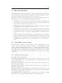
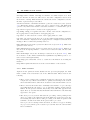
FIES Automatic Data Reduction Software
version 1.0
User Manual
Eric Stempels
November 24, 2005
CONTENTS
3
Contents
1 Introduction
5
2 Software installation
6
2.1
System requirements . . . . . . . . . . . . . . . . . . . . . . . . . . .
6
2.2
Packages to be installed . . . . . . . . . . . . . . . . . . . . . . . . .
6
2.3
Unpack and install the software . . . . . . . . . . . . . . . . . . . . .
7
2.4
Getting started . . . . . . . . . . . . . . . . . . . . . . . . . . . . . .
7
2.4.1
Starting the software . . . . . . . . . . . . . . . . . . . . . . .
7
2.4.2
Initial configuration . . . . . . . . . . . . . . . . . . . . . . .
7
2.4.3
Installing pre-calculated reference data . . . . . . . . . . . . .
8
3 The user interface
3.1
9
The FIEStool main window . . . . . . . . . . . . . . . . . . . . . . .
9
3.1.1
Pull-down menu options . . . . . . . . . . . . . . . . . . . . .
9
3.1.2
Other elements . . . . . . . . . . . . . . . . . . . . . . . . . .
11
Configuration Frame . . . . . . . . . . . . . . . . . . . . . . . . . . .
12
3.2.1
Pipeline Configuration Frame . . . . . . . . . . . . . . . . . .
15
3.3
Calibration Frame . . . . . . . . . . . . . . . . . . . . . . . . . . . .
17
3.4
AutoLoader Frame . . . . . . . . . . . . . . . . . . . . . . . . . . . .
17
3.2
4 Implemented data-reduction routines
4.1
4.2
19
Data-reduction modes . . . . . . . . . . . . . . . . . . . . . . . . . .
19
4.1.1
Quicklook . . . . . . . . . . . . . . . . . . . . . . . . . . . . .
19
4.1.2
Advanced . . . . . . . . . . . . . . . . . . . . . . . . . . . . .
20
4.1.3
DoubleSpec . . . . . . . . . . . . . . . . . . . . . . . . . . . .
20
4.1.4
CalibCalc . . . . . . . . . . . . . . . . . . . . . . . . . . . . .
21
Data reduction tasks (steps) . . . . . . . . . . . . . . . . . . . . . . .
21
4.2.1
Autoload configuration . . . . . . . . . . . . . . . . . . . . . .
22
4.2.2
Preprocess frame . . . . . . . . . . . . . . . . . . . . . . . . .
22
4.2.3
Subtract BIAS . . . . . . . . . . . . . . . . . . . . . . . . . .
22
4.2.4
Subtract scattering . . . . . . . . . . . . . . . . . . . . . . . .
22
4.2.5
Divide by 2-D flat . . . . . . . . . . . . . . . . . . . . . . . .
22
4.2.6
Plot cross-order profile . . . . . . . . . . . . . . . . . . . . . .
23
4.2.7
Determine spectrum shift . . . . . . . . . . . . . . . . . . . .
23
4.2.8
Extract spectrum . . . . . . . . . . . . . . . . . . . . . . . . .
23
4.2.9
Correct for blazeshape . . . . . . . . . . . . . . . . . . . . . .
23
4.2.10 Add wavelengths . . . . . . . . . . . . . . . . . . . . . . . . .
23
4.2.11 Adjust wavelengths . . . . . . . . . . . . . . . . . . . . . . . .
23
4.2.12 Merge orders . . . . . . . . . . . . . . . . . . . . . . . . . . .
24
4.3
4.2.13 Autoplot reduced spectra . . . . . . . . . . . . . . . . . . . .
24
Tasks to calculate reference frames . . . . . . . . . . . . . . . . . . .
24
4.3.1
Create combined BIAS . . . . . . . . . . . . . . . . . . . . . .
24
4.3.2
Create combined FLAT . . . . . . . . . . . . . . . . . . . . .
24
4.3.3
Find order locations . . . . . . . . . . . . . . . . . . . . . . .
24
4.3.4
Find interlaced order locations . . . . . . . . . . . . . . . . .
25
4.3.5
Plot order locations . . . . . . . . . . . . . . . . . . . . . . .
25
4.3.6
Create normalized combined FLAT . . . . . . . . . . . . . . .
25
4.3.7
Find wavelength solution . . . . . . . . . . . . . . . . . . . .
25
4.3.8
Find interlaced wavelength solution
26
. . . . . . . . . . . . . .
5 Calculating reference data
27
5.1
A complete set of reference data . . . . . . . . . . . . . . . . . . . .
27
5.2
Needed input frames for calculating reference data . . . . . . . . . .
27
A Program structure and description of files
29
B Default IRAF parameter files
31
C Modifying the software
32
C.1 Adding and removing reduction tasks . . . . . . . . . . . . . . . . .
32
C.2 Changing reduction tasks . . . . . . . . . . . . . . . . . . . . . . . .
32
C.3 Changing configuration options . . . . . . . . . . . . . . . . . . . . .
33
C.4 Finally . . . . . . . . . . . . . . . . . . . . . . . . . . . . . . . . . . .
33
5
1
Introduction
Reducing echelle data can be a time-consuming process, especially if it is the first
time an observer obtains data from a new instrument. Data reduction is also not
what an observer wants to be spending time on during an observing run. However,
to be able to make strategic decisions during an observing run, data reduction
during observations is essential. In particular, it is important to get a quick first
impression of the data. For these reasons, there is a strong desire for the automatic
reduction of data already at the telescope.
FIES (FIber-fed Echelle Spectrograph) at the Nordic Optical Telescope is a highresolution spectrograph, available on a stand-by basis. This means that an observer
has the possibility to execute observing programs that need flexible scheduling, such
as long-term studies of objects with day-to-day variability, or target-of-opportunity
programs that require a high-resolution spectrograph to be available. It is very
likely that such programs will be executed in service mode. Automatic reduction
of observations will then be an important complement to such observing modes.
Automatic reduction also standardizes the reduction procedure and will simplify
the user’s effort by offering a default setup of reduction parameters
This document describes the software package FIEStool, developed just for this purpose. FIEStool is written in Python, an object-oriented language that provides easy
interfacing between the user, through a Graphical User Interface, and specialized
reduction tasks from the external packages IRAF and NumArray, both developed
at STScI. It is capable of automatically reducing data obtained with FIES, while
at the same time providing the user the possibility to control the basic properties
of the reduction process by hand.
An important requirement when developing this software was that it should be flexible, so it will be possible to adapt the software to future changes in the data format
or instrument characteristics. In fact, the core of FIEStool is written completely
instrument-independent, so that the software could, with minor modifications, also
be used for automatic reduction of data from other instruments.
This manual gives a detailed description of the user interface and the underlying
routines, as well as instructions on how to modify the software if that would be
necessary. Still, the only way to really learn how to use FIEStool for data reduction,
is by using it.
6
Software installation
2
Software installation
2.1
System requirements
FIEStool was developed on a 2.4 GHz computer with 512 MB of memory, running
a Linux system (RedHat 7.3 with some updated packages). As these is a rather
moderate configuration, the software should run on any modern Linux distribution.
2.2
Packages to be installed
In order to be able to run FIEStool, one will need at least the following standard
software packages to be installed. These packages are availble (as RPMs or similar)
from standard Linux distributions.
• python v2.3 or better
• python-dev
• python-tk
• python-Numeric
• f2c
• libplot-devel
• X
• X-devel
The reduction package uses some routines of IRAF (http://iraf.noao.edu/). Therefore, a working installation of IRAF is required. This software was developed using
IRAF version 2.12.2. Installing IRAF is beyond the scope of this manual; please
take a look at the instructions that come with IRAF.
In addition to the mentioned software packages, one will need to download and
install the following Python modules (version numbers are the minimum required):
• Numarray v0.9
http://www.stsci.edu/resources/software hardware/numarray/
• PyFITS v0.9
http://www.stsci.edu/resources/software hardware/pyfits/
• PyRAF v1.1.1
http://www.stsci.edu/resources/software hardware/pyraf/
• Biggles 11.6.4
http://biggles.sourceforge.net/
Instead of installing Numarray, PyFITS and PyRAF seperately, it is also possible
to install STScI-Python :
• STScI-Python v2.0
http://www.stsci.edu/resources/software hardware/pyraf/stsci python
2.3
Unpack and install the software
7
This is a bundle of Python packages that contains, among others, Numarray, PyFITS and PyRAF.
Python packages can either be installed system-wide, or as a local-user installation.
In case the latter option is chosen, it is important to set the system environment
variable PYTHONPATH to the directory under which the packages resort.
Please refer to the respective web-pages for information on the installation of these
packages.
2.3
Unpack and install the software
FIEStool is available as a gzipped tar-archive. Unpack this archive in a suitable
directory. As python is an interpreted scripting language, there is no need to compile
the software; this will be done on-the-fly the first time the software is started.
It is necessary to initialize IRAF in the same directory as in which the reduction
software is installed. This is accomplished by issuing ’mkiraf’ in this directory
(choice of terminal type is not critical). This will generate the file login.cl. This file
should then be edited to make the default image format ’fits’, instead of ’imh’ :
set imtype = "fits"
2.4
Getting started
This section gives a short overview of how to start FIEStool for the first time after a
new install. More detailed explanations of the functionality of the software is given
in the next sections.
2.4.1
Starting the software
Once installation has been completed, running the reduction software is straightforward. From the prompt, invoke the main routine of the package
> ./FIEStool.py
and the Graphical User Interface (GUI) will appear. Do not run the program in
the background, and do not exit the terminal window in which the program was
started. Sometimes, useful messages will be echoed to this window.
The program can also be started with the command line option -c or --calib.
This will enable the possibility to calculate new configuration data and should only
be used when this really is desired.
2.4.2
Initial configuration
If you are doing a new installation of the software, it is important to do some initial
configuration. Start FIEStool with the extra command-line option:
> ./FIEStool.py -c
Then choose separate directories for input, output and reference data frames, and
enter these locations in the configuration of the interface (see section 3.2 for more
details about this). You also will have to decide on the names of reference frames
that will be created when calculating a new set of reference data. When these
options have been configured you may want to save the current configuration as the
default configuration (see section 3.1.1).
8
Software installation
Before you will be able to perform data reduction you will need to create a set
of reference frames, or download a previously calculated set. A new set can be
calculated by executing, from top to bottom, all the tasks in the calibration frame
(see section 5 for more details).
2.4.3
Installing pre-calculated reference data
As the FIES spectrograph is very stable, it is possible to use pre-calculated reference
data.1 These data can be downloaded from the FIES instrument homepage. There
you can also find instructions on how to install these files.
1 Because of the current state of the instrument, no such data has been calculated yet. After
improvement of the instrument these data will be made available (051124).
9
3
The user interface
The graphical user interface is designed to be as self-explanatory as possible. Most
buttons and fields contain on-line help information, accessible through popup windows when clicking with the right mouse button on an item.
The interface consists of four different windows. A detailed description of these four
windows is given in the next paragraph. The four windows are:
• The FIEStool main window is used to perform the automated data reduction
and allows to do some quicklook plotting of the reduced spectra. This is the
only window is visible from startup (section 3.1).
• The Configuration window allows the user to view and modify all the available
configuration options of the interface (section 3.2).
• The Calibration window allows to prepare all the necessary reference frames
(such as normalized flats, descriptions of the blaze shape and wavelength solutions) that are needed to properly process the stellar (object) frames (section
3.3).
• The AutoLoader window allows the user to configure the interface to automatically load a set of reference data when starting to process a new frame. The
interface will base its decision to be load reference data on the actual values of
the FITS header keywords of the object frame that is to be processed (section
3.4).
3.1
The FIEStool main window
The main window of FIEStool, shown in Figure 1, is the central interface between
the user and the data reduction routines. It allows to access other frames of the
interface (discussed in subsequent sections), to control the data reduction steps, to
start and stop data reduction and to review the obtained results. It also contains
the logging window, in which diagnostic information is shown about the progress
and status of the data reduction routines. This window consists of the following
components.
3.1.1
Pull-down menu options
File->Quit quits the application.
Settings->Configure pipeline opens the Pipeline configuration frame (section
3.2.1). This frame allows to edit a limited number of settings, all related to the
pipelined data reduction.
Settings->Load pipeline config loads a previously saved set of pipeline configuration settings from disk.
Settings->Save pipeline config saves the currently active set of pipeline configuration settings to disk.
Settings->Configure autoloading opens the AutoLoader frame (section 3.4).
This frame allows to configure the automatic loading of pipeline settings depending
on the values of FITS header keywords.
Settings->Edit all settings opens the Configuration frame (section 3.2). This
frame allows to consult and edit all the available configuration options.
10
The user interface
Figure 1: Screenshot of the main window of FIEStool (section 3.1)
3.1
The FIEStool main window
11
Settings->Save current settings as default does what is says it does. Next
time the interface is started, it will revert to the same configuration as it is in at
the moment of saving. This includes the current autoloader configuration, but not
the lists of queued and processed files.
Calibs->Calculate calibration frames opens the Calibration frame (section
3.3). This frame allows to calculate new sets of reference data. NB: This menu
option is only visible if the interface was started with the -c command line option.
Log->Clear log deletes the contents of the logging window.
Log->Dump config to logfile writes the contents of the current configuration to
the logging window. Only useful for debugging purposes.
Log->Save to file saves the content of the logging window to disk.
Log->Set log level lets the user choose in how much detail messages, warnings
and errors should be displayed in the logging window. A higher level means more
messages. The recommended (default) value is 5.
Mode->Quicklook selects the Quicklook reduction mode (section 4.1.1). This is the
quickest reduction mode.
Mode->Advanced selects the Advanced reduction mode (section 4.1.2). This mode
uses more thourough algorithms to obtain a better reduction result, but also takes
more time.
Mode->DoubleSpec selects the DoubleSpec reduction mode (section 4.1.3). This
mode allows to reduce frames with interlaced (simultaneous) ThAr spectra, to obtain a better wavelength stability.
Help->Help gives a first hint on how to obtain more information about using the
interface.
Help->About prints information about the version number of the software.
3.1.2
Other elements
Apart from the pull-down menu discussed in the previous paragraph, the main
frame consists of five areas that focus on five different tasks. These areas are the
following.
• The top area consists of the configuration buttons for the Input directory and
Output directory. These buttons allow to quickly set and inspect the location
where raw frames will be taken from, and where reduced frames will be stored.
• The second area allows the user to manually select frames to be processed (by
appending them into the queue), or to do automatic queuing of newly reduced
frames. If AutoQueue is enabled, Any newly created file that appears in the
input directory and that matches the filename filter will then be automatically
appended to the queue.
• The Start processing button will start the processing of files pending in the
queue, according to the tasks selected in the third area. If an error is encountered during any data reduction task, processing of the frame in question will
terminate, and the next frame in the queue will be processed.
Once a process of reducing a frame is started, it cannot be stopped. Pressing
Stop processing will stop the reduction process first after the current frame
has been finished.
12
The user interface
• The forth area allows the user to control some plot parameters, such as which
wavelength range is to be plotted, or, if no wavelength information is available,
which spectral order . Automatic plotting of spectra will always use routines
from the Biggles plotting package, because plotting with IRAF would interrupt
the continuous processing of frames. However, once the reduction of a frame
is finished, one can use IRAF-based plotting routines (using echelle.splot) to
investigate the spectrum.
• The fifth area contains the logging window, showing the progress and status
of the reduction interface.
3.2
Configuration Frame
The configuration frame consists of one large panel that allows to edit and review
the values of all available configuration options. The available options are listed
below.
The first two options define the name of the default input and output directories.
Input directory determines from which directory raw frames are read, and is also
the directory that is monitored when the AutoQueue feature is enabled. This option
can also be reviewed from the FIEStool main window.
Output directory determines in which directory the resulting reduced frames, including intermediate products, are stored. This option can also be reviewed from
the FIEStool main window.
The following six options allow the selection of input files for the calculation of
calibration (reference) frames.
List of BIAS frames allows to select one or more frames from the input directory
that will be used by the Calibration frame (Sect. 3.3) to calculate a combined BIAS
frame. This option can also be reviewed from the Calibration frame.
List of FLAT frames allows to select one or more frames from the input directory
that will be used by the Calibration frame (Sect. 3.3) to calculate a combined FLAT
frame. This option can also be reviewed from the Calibration frame.
Order definition frame is a well-exposed frame that will be used by the Calibration frame to detect the location of the spectral orders. This option can also be
reviewed from the Calibration frame.
Wavelength definition frame is a frame containing an emission line lamp spectrum, which will be used to determine the 2-dimensional wavelength solution of the
echelle frame. This option can also be reviewed from the calibration frame.
Interlaced order definition frame is similar to the Order definition frame, except that it will trace the interlaced spectral orders. Interlaced spectra are normally
used to obtain a simultaneous wavelength reference spectrum (ThAr). This option
can also be reviewed from the Calibration frame.
Interlaced wavelength definition frame is similar to the Wavelength definition frame, except that it will provide the 2-dimensional wavelength solution for the
interlaced orders. This option can also be reviewed from the Calibration frame.
The following ten options allow to select the filenames of reference frames. In the
Calibration frame reference files are calculated, so these filenames below refer to the
produced output files. On the other hand, these frames are also used as reference
frames when performing the reduction of a stellar (science) frame, and are thus in
that sense input files. Therefore, for a working data reduction one will have to have
valid reference files defined and prepared.
3.2
Configuration Frame
Figure 2: Screenshot of the Configuration Frame (section 3.2)
13
14
The user interface
Reference directory is the directory in which the reference files can be found.
Bad pixel mask is a frame, of identical size and format as the raw data frames,
with pixel values of 1 for good pixels and 0 for bad pixels. This is the only frame
that can not be calculated by FIEStool.
Combined BIAS frame is an averaged and filtered version of a large number of BIAS
frames.
Combined FLAT frame is an averaged version of a large number of FLAT frames.
Normalized combined FLAT frame is similar to the combined FLAT frame, except
that the response across the spectral orders (in the ‘spatial’ direction) and along the
order has been removed. Dividing by this frame compensates for the pixel-to-pixel
variations in sensitivity.
Fitted blaze shape is the shape of the extracted orders of the combined FLAT
(also called blaze). This response was removed from the combined FLAT field when
calculating the Normalized combined FLAT frame. Dividing the extracted orders
of an object frame by this frame will remove the signature of the blaze from the
spectra.
Order definition reference frame is similar to (and often a direct copy of) the
order definition frame defined above, but with overscan regions removed and a valid
order definition attached to it.
Wavelength reference frame is similar to (and often a direct copy of) the wavelength definition frame, but with overscan regions removed and a valid 2-dimensional
wavelength definition attached to it.
Master wavelength reference frame is similar to the wavelength reference frame.
The wavelength definition of this frame will be used as a first guess (a master) when
determining a new wavelength solution for the wavelength reference frame.
Interlaced order definition reference frame is similar to the order definition reference frame, but for the interlaced spectral orders.
Interlaced wavelength reference frame is similar to the wavelength reference
frame, but for the interlaced spectral orders.
The following three options control the internal behaviour of the interface, and need
seldom to be adjusted.
Listed FITS headers is a space-separated list of FITS header card names that
will be displayed in the file dialog when editing the contents of the queue of frames
awaiting reduction. Only a couple of keywords should be given here, because a large
number of keywords will cause delays when displaying the file listing.
MEF data extension is the number of the Multi-Extension FITS (MEF) Header
Data Unit that contains the echelle data. In case the input spectra are not in MEFformat, or if the data is in the primary Header Data Unit, this value should be 0.
Currently, FIES produces files with the echelle data in MEF unit 1.
Frame orientation defines how the input frames should be rotated and/or flipped.
FIEStool assumes that the data is oriented in such a way that the wavelengths
increase along the X- and Y-axis, and that the orders run along the Y-axis. A
value of 0 means that no initial rotation or flipping is done. A value of 1, 2 or 3
corresponds to a rotation of 90, 180 and 270 degrees, respectively. The values of 4,
5, 6 and 7 are similar to 0, 1, 2 and 3, but with an additional transposition of the
image. The current format of the frames produced by FIES requires a value of 7
for proper reorientation.
Config file directory is the directory in which configuration files (generated by
this frame) and pipeline configuration files (see 3.2.1) are located.
3.2
Configuration Frame
15
Figure 3: Screenshot of the Pipeline Configuration Frame (section 3.2.1)
IRAF tasks config directory is the directory in which complete task definitions
for the implemented IRAF tasks are stored.
The next four options control the useful area of the CCD. These options allow the
user to define personal preferences on which area should be processed, rather than
to use pre-defined values from the image headers. These numbers refer to the frame
pixel numbers after a possible reorientation. If these options are changed, a new
and complete set of reference frames must be generated before reduction will work
properly again.
x_start is the number of the first useful x-pixel in the frames
x_end is the number of the last useful x-pixel in the frames
y_start is the number of the first useful y-pixel in the frames
y_end is the number of the last useful y-pixel in the frames
The buttons Save settings and Load settings allow the user to save and restore sets of
configuration options to and from disk. Pressing Reset will revert the configuration
options to the most recently saved or loaded settings.
3.2.1
Pipeline Configuration Frame
When reducing a dataset that contains different readout modes, for example different binning or amplifier settings, one will also have to use a different set of
reference frames. In order to make is easier to switch between different sets of reference frames, one can use the Pipeline configuration frame. This frame allows to
edit, load and save the relevant options.
The advantage of using the Pipeline configuration frame above the (normal) configuration frame is that the load and save options only operate on the displayed subset
of options, and nothing else. In this way one can develop a set of configuration files
for the different readout modes, and load the relevant options when starting to
reduce data with a different readout mode.
The pipeline configuration files that can be constructed in this way can also be
used in combination with the automatic configuration file loader, the AutoLoader,
16
The user interface
Figure 4: Screenshot of the Calibration Frame (section 3.3)
3.3
Calibration Frame
17
described in section 3.4. The AutoLoader decides on loading configuration files
based on the contents of FITS headers.
3.3
Calibration Frame
The Calibration frame allows the user to easily calculate reference data, such as
combined BIAS frames, combined FLAT frames, and order and wavelength reference
frames. The upper part of the frame lists all configuration options that are relevant
for calculating these frames. More details on these options can be fount in section
3.2. The lower part contains a set of buttons that, when pressed, will perform one
particular step in constructing reference data. These tasks are typically performed
in the order listed below.
Create combined BIAS will calculate an average BIAS frame (called Combined
BIAS frame) from a selection of observed BIAS frames. See 4.3.1.
Create combined FLAT will calculate an average FLAT frame (called Combined
FLAT frame) from a selection of observed FLAT frames. See 4.3.2.
Find Order Locations will locate and trace the spectral orders in the specified
order definition frame. See 4.3.3.
Find Interlaced Order Locations is similar to the previous task, except that it
will trace the location of interlaced orders. See 4.3.4.
Plot order locations provides a visual check of the location of the spectral orders
on the CCD according to the latest calculated order and interlaced order locations.
This task generates no output. See 4.3.5.
Create normalized flat will calculate a 2-dimensional model of the pixel responses, based on the Combined FLAT frame. See 4.3.6.
Find wavelength solution will determine a solution to the 2-dimensional dispersion function from a wavelength definition frame (usually a ThAr spectrum). See
4.3.7.
Find interlaced wavelength solution is similar to the previous task, but for
the interlaced spectrum. See 4.3.8.
3.4
AutoLoader Frame
The automatic configuration loader, or for short AutoLoader, allows the user to
create a set of logical conditions (rules) using the values of FITS header keywords
and, depending on the outcome of these rules, automatically load configuration
files. In this context, the pipeline configuration files (section 3.2.1) are extremely
useful, because these files contain only configuration options relevant to reference
data. The autoloader is intended to make it easier to automatically reduce sets of
data that contain mixed readout modes, for example different binning factors or
amplifiers.
Defining rules is relatively straightforward. The FITS header field should contain
the name of the FITS header keyword that is to be evaluated. The expression defined in Expression is a standard Python expression, for example == 2, or > 7, that
will be parsed together with the value of the corresponding FITS header keyword.
The actions defined in If true or If false are either a number (of the next rule
to branch to), or the word ‘load’ (load a configuration file and stop parsing rules),
or nothing (do nothing and stop parsing rules). A name of a configuration file can
be given in the field Pipeline configuration file, which only is relevant if one
of the defined actions for this rule was ‘load’.
18
The user interface
Figure 5: Screenshot of the AutoLoader Frame (section 3.4)
Once a set of rules has been defined, it can be tested against a sample frame. The
action that would have been performed will be reported in a popup-window. If for
some reason no action could be performed, due to an error or lack of rules, this will
also be shown in a popup-window.
A set of rules defined here can only be saved to disk as part of the default configuration file. It would not make sense to save the set of rules as part of a normal
configuration file, or even worse as part of a pipeline configuration file, because this
would lead to changing sets of rules while processing data, and thus to unexpected
or at the least very confusing behaviour.
Using the autoloader to load configuration files is one of the default tasks when
running the automatic data reduction. Note that although autoloading may fail, it
will never suspend the reduction of a frame.
19
4
Implemented data-reduction routines
Although the reduction of echelle spectra requires a large number of steps, these
steps are well-defined. The process can also easily be repeated for a large number of
frames, mainly because the position of the spectrum in the two-dimensional frame
is more or less fixed over time. This greatly simplifies the extraction and calibration
procedures, and allowed to develop this reduction package.
The typical reduction steps involved in echelle data reduction are BIAS subtraction,
flat-field normalization, extraction of the spectra and the assignment of wavelengths
along the spectra. The reduction can be made more accurate or more extended by
including more steps in the reduction, such as the subtraction of scattered light or
merging of the spectral orders.
Because the reduction process can be divided into such well-defined steps, this
reduction package has at its core part a set of reduction tasks. These tasks perform
one single step of the reduction process, for example subtract scattering. With
subsequent execution of the individual tasks one can then perform the complete
reduction of an echelle spectrum. In the package, the tasks needed for a complete
reduction are grouped together and ordered into data-reduction modes. Which tasks
that together make up each mode depends on the particular requirements for that
mode (e.g. speed for quick-look data reduction). Therefore one single task may be
part of several reduction modes. Currently, there are four data-reduction modes
implemented, named QuickLook, Advanced, DoubleSpec and CalibCalc.
Around the different tasks and data-reduction strategies is a software layer that
controls the order and execution of the individual tasks within each data-reduction
mode. This outer later is visualized and controlled by the user through the Graphical User Interface (GUI). With this GUI the user can select the preferred datareduction mode, (de)select the tasks within the mode, and perform the actual data
reduction.
When the tasks that constitute a reduction mode are executed, FIEStool will write
the result of each reduction task to disk, allowing the user to later review these
intermediate steps. Also, all operations that were performed on a frame are written
to the FITS header keyword HISTORY.
Below follows an overview of the different reduction modes, together with more
detailed descriptions of each task.
4.1
4.1.1
Data-reduction modes
Quicklook
The Quicklook data reduction mode is optimized for speed. It contains few steps,
which all are performed without optimization. The execution of all tasks takes only
a few seconds. The results of this mode are only intended to give the observer a first
impression of the observed spectrum and should not be used for further analysis.
The included tasks are :
• Autoload configuration
• Preprocess frame
• Subtract BIAS
• Divide by 2-D flat
20
Implemented data-reduction routines
• Plot cross-order profile
• Extract spectrum
• Correct for blazeshape
• Add wavelengths
• Autoplot reduced spectra
4.1.2
Advanced
The Advanced data reduction mode is optimized for quality, at the expense of speed.
The execution of all tasks takes about one minute. Some tasks, such as subtract
scattering and merge orders are very cpu-intensive and time-consuming. Because
this reduction mode performs the tasks in an optimal way, the results can be used
for spectral analysis.
A list of tasks is presented below. Note that there exists no task for continuumfitting included, because this is a very subjective reduction step and depends on the
particular needs of the scientific project.
• Autoload configuration
• Preprocess frame
• Subtract BIAS
• Subtract scattering
• Divide by 2-D flat
• Plot cross-order profile
• Extract spectrum
• Correct for blazeshape
• Add wavelengths
• Merge orders
• Autoplot reduced spectra
4.1.3
DoubleSpec
The Doublespec reduction mode takes into account that the frame contains both
an object spectrum and an interlaced wavelength calibration spectrum (normally
ThAr). This additional wavelength spectrum allows to correct for possible instrumental shifts, improving the wavelength calibration. High-quality wavelength calibrations are important for radial-velocity studies.
The performance of this data reduction mode is comparable to the Advanced mode.
The included tasks are listed below. Order merging is not included because it
involves resampling of the wavelenghts on a common (monospaced) wavelength
grid, which may reduce the quality of the wavelength calibration.
• Autoload configuration
4.2
Data reduction tasks (steps)
21
• Preprocess frame
• Subtract BIAS
• Subtract scattering
• Divide by 2-D flat
• Plot cross-order profile
• Determine spectrum shift
• Extract spectrum
• Correct for blazeshape
• Add wavelengths
• Adjust wavelengths
• Autoplot reduced spectra
4.1.4
CalibCalc
The CalibCalc reduction mode is a special mode that is optimized for calculating
reference data, such as combining biases and flat fields, order finding and tracing
and wavelength calibration. This mode is automatically enabled when the user
starts tasks from the ’Calibration frame’ (see section 3.3). Differing from the other
reduction modes, these tasks are not automatically executed together. Instead, the
user will have to execute these one at a time. The tasks included in this mode are :
• Create combined BIAS
• Create combined FLAT
• Find order locations
• Find interlaced order locations
• Plot order locations
• Create normalized combined FLAT
• Find wavelength solution
• Find interlaced wavelength solution
4.2
Data reduction tasks (steps)
Below follows a short description of each of the data-reduction tasks. More detailed
information on the calculations can be found in the comments of the source code.
The tasks make use of two external packages for calculations. Numerical array operations on frames or subsets of frames are performed with the NumArray package,
while specific echelle reduction tasks (for example, optimal order extraction) are
performed with IRAF. In the case a tasks calls IRAF to do the work, IRAF parameter configuration files are used to determine the behaviour of the IRAF tasks (see
the appendix about the location of these files). Plotting is done either by the Biggles plotting package (for non-interactive plotting), or the IRAF task echelle.splot
(interactive).
22
Implemented data-reduction routines
4.2.1
Autoload configuration
This task executes the rules defined by the AutoLoader (see section 3.4), loading
configuration files depending on the value of FITS header keywords of the frame that
is being processed. The absence of any rules or the failure to execute the ruleset
will only generate a warning and not interrupt the current reduction. This task
is particularly useful for changing the used set of reference data (combined flats,
location of the spectral orders) when reducing sets of data with different binnings.
4.2.2
Preprocess frame
Before any more tasks are performed on a frame it will be ’preprocessed’. This task
does the following substeps :
• Extract the data block if the frame is in Multi-extension FITS format.
• Check the integrety of the FITS headers.
• Clip and rotate/flip the frame so that overscan regions are removed and the
orders run vertically (NumArray). This is necessary for later processing by
IRAF.
• Extend the frame to full size if it was windowed (NumArray). This strongly
simplifies the data reduction of windowed frames.
• Remove bad pixels using a bad pixel mask, where 1 = good pixel and 0 = bad
pixel (NumArray).
• Calculate the heliocentric velocity correction (IRAF: astutil.rvcorrect) and
store it in the header keyword VHEL. Note that this information is only stored
in the header and not used when adding a wavelength definition to the spectrum.
4.2.3
Subtract BIAS
This tasks subtracts the combined BIAS frame from the observerd frame (NumArray).
4.2.4
Subtract scattering
Using the level of light in the inter-order spaces, this task determines a 2-dimensional
model of scattered light (IRAF: echelle.apscatter). Thereafter, it subtracts the
scattered light image from the observed frame (NumArray).
4.2.5
Divide by 2-D flat
This will divide the observed frame by the normalized 2-dimensional flat, removing
signatures of 2-dimensional fringes in the image (NumArray).
4.2
Data reduction tasks (steps)
4.2.6
23
Plot cross-order profile
This is a task that does not do any operations on the frame. It only plots the
average of the central 10 rows of the frame, in order to give the user an estimate of
the quality of the exposure, whether any orders are overexposed and how well the
subtraction of scattered light was performed (extraction by NumArray, and plotting
by Biggles).
4.2.7
Determine spectrum shift
By comparing the extracted spectra (IRAF: echelle.apsum) of the default interlaced wavelength solution and the interlaced wavelength spectrum in the object
frame, one can obtain an estimate of the shift in the wavelength solution (IRAF:
echelle.ecreidentify). The determined wavelength shift (in the zeroth order) is then
written to the FITS header keyword WVLSHIFT, so that it can be used when attaching the wavelength calibration to the extracted spectrum. If less than 10% of
the lines in the spectrum could be identified, the comparison is assumed to have
failed and no shift will be written to the FITS headers.
4.2.8
Extract spectrum
This task will extract the individual orders into one-dimensional spectra from the
observed frame using optimal extraction (IRAF: echelle.apsum). In case the chosen
reduction mode is Advanced, DoubleSpec, or CalibCalc, rejection of deviant pixels
is performed using the ‘clean’ algorithm of IRAF’s echelle.apsum, yielding a cleaner
spectrum but requires more processing time.
4.2.9
Correct for blazeshape
This will divide the extracted object spectrum by the blaze shape of the combined
FLAT, removing the blaze shape from the object spectrum (NumArray). This
method of double flat-fielding, by first dividing the non-extracted frame by a normalized (=unblazed) 2-dimensional flat, and later the extracted spectra by the blaze
shape of the flat-field spectrum yields much better results than applying only one
single flat-field division.
4.2.10
Add wavelengths
This task will attach the wavelength solution of the wavelength reference frame to
the one-dimensional object spectra (IRAF: iraf.dispcor).
4.2.11
Adjust wavelengths
This task2 is only used with the reduction mode DoubleSpec. It will apply a shift
in the attached wavelength definition of each order using the earlier determined
zeroth order wavelength offset from Determine spectrum shift, converted to the
appropriate value for each order (IRAF: onedspec.sapertures). In this way one
obtains a wavelength definition that is not degraded by instrument drifts during
the night.
2 Adjust wavelengths has not been tested due to the non-availability of the interlaced spectra in
the existing setup (051124)
24
4.2.12
Implemented data-reduction routines
Merge orders
Merges the individual spectral orders into one long 1-dimensional spectrum (IRAF:
echelle.scombine). In the regions where consecutive spectral orders overlap in wavelength, the spectra are averaged. Because the dispersion in individual orders is different, merging implies rebinning on a new wavelength grid and may decrease the
actual spectral resolution. Also, rebinning means that the flux (counts/wavelength
bin) is not conserved.
4.2.13
Autoplot reduced spectra
After the reduction of a frame is finished, this option allows to automatically plot
a selected region of the extracted spectrum. The plotted wavelength range is determined by the values entered below this option. A value of 0 as the minimum or
maximum wavelength will be interpreted as the minimum or maximum available
wavelength. Automatic plotting is always done using the Biggles plotting package,
because IRAF plots are interactive and would interrupt the continuous reduction
of frames.
4.3
Tasks to calculate reference frames
The following tasks are only performed when calculating new reference data, and
are thus part of the CalibCalc reduction mode. These tasks are stand-alone and are
invoked one by one by the user. When creating a new set of reference data from
scratch, one should execute the tasks in the order shown below, because the later
tasks may require results from some of the earlier tasks.
4.3.1
Create combined BIAS
Using a (preferably large) number of BIAS frames, this task will calculate an averaged (combined) BIAS frame. Using the statistics of the BIAS frames, it will
determine which pixels of the set are deviating by more than 5σ from the average
BIAS level and replace these pixels with average BIAS values (all using NumArray),
thus removing signatures from cosmic rays.
4.3.2
Create combined FLAT
This task will combine the selected FLAT frames into one average (combined) FLAT
frame (NumArray). No rejection techniques like the one used for the BIAS frames
is included. Rejection of deviant pixels will be performed later, when modelling the
shape of the orders, in the task Create normalized combined FLAT below.
4.3.3
Find order locations
Using a well-exposed flat-field or object frame, this task will invoke the IRAF task
echelle.apfind and echelle.apedit and let the user interactively define the location of
the spectral orders and the regions sampling the background level from the interorder gaps. After the user finishes defining the order location, the task will call
IRAF’s echelle.aptrace to trace the order locations and attach this definition to the
order definition reference frame (a rotated and clipped copy of the order definition
frame).
4.3
4.3.4
Tasks to calculate reference frames
25
Find interlaced order locations
This task is in general terms similar to the previous task, except that it is not interactive and will determine the location of the interlaced orders. Interlaced spectra
can be useful for improved wavelength stability or the observation of background
(sky) spectra. The input frame, the interlaced order definition frame, should therefore be a well-exposed flat-field or object frame with only the interlaced spectrum
present. The task will determine the shift of the order locations with respect to
the non-interlaced order definition when finding the interlaced orders, and does not
perform any new order-tracing.
4.3.5
Plot order locations
This task is only a diagnostic tool for the user, showing the location of the traced
orders on the CCD. If the orders could not be traced properly, this will be evident
from this plot. If an order definition of the interlaced orders exists, the interlaced
orders will be plotted in the same figure, but with a different color.
4.3.6
Create normalized combined FLAT
This is a very extensive task that produces two important products for proper
echelle data reduction. First of all, it will subtract the scattered light from the
combined FLAT frame (IRAF: echelle.apscatter). The result is used to determine
the 2-dimensional shape of each spectral order in the combined FLAT. These profiles, describing the order shape both along the blaze and along the direction of
cross-dispersion, are then used to determine the responses of the individual pixels
that constitute the spectral orders (IRAF: echelle.apnormalize). This yields the
2-dimensional normalized combined FLAT. Dividing an object frame by this normalized flat is a very effective method to reduce fringing in the CCD. Fringing is
strongly wavelength dependent, which is why scattered light should be subtracted
first.
In the next step the combined FLAT is divided by this 2-dimensional normalized
combined flat (NumArray), and its orders, now smooth, are extracted with IRAF’s
echelle.apsum. This yields the blaze shape that is present in all extracted spectra.
This instrumental signature can then be easily removed from any extracted object
spectrum by dividing by this blaze shape. In order to accurately describe the blaze
shape, noise due to pixel-to-pixel differences in response is suppressed by smoothing
the blaze shape with a 3-pixel wide Gaussian-shaped filter (NumArray). Those
regions of the function describing the blaze shape that are not well exposed, with
signal-to-noise ratios of less than 100, are then replaced by a smooth fitted curve
(fitting by IRAF’s imfit.fit1d, replacing by NumArray). This will avoid degradation
of the signal-to-noise when dividing extracted spectra from well-exposed object
frames by the fitted blaze shape.
4.3.7
Find wavelength solution
After very simple extraction of the spectrum (collapsing the orders along the crossdispersed direction), this task will allow the user to interactively determine the
wavelength solution from the wavelength definition frame (IRAF: echelle.ecidentify).
If a master wavelength definition frame was defined in the set of configuration
options, the solution corresponding to that frame is used as the initial solution when
determining the wavelength definition. Upon leaving the interactive interface, the
26
Implemented data-reduction routines
rotated and clipped wavelength definition frame is stored as the reference wavelength
definition frame, and the determined wavelength solution is attached to it. If one is
very confident about the obtained wavelength solution, this frame can be renamed
as the master wavelength reference frame and thus provide a future initial guess.
4.3.8
Find interlaced wavelength solution
This task is very similar to the previous task, except that it does not need interaction
with the user. The non-interlaced wavelength solution is used as the initial solution
to the interlaced wavelength definition spectrum, and IRAF’s echelle.reidentify is
used to adapt (shift and refit) the wavelength solution to the extracted spectra of
the interlaced wavelength definition frame. The determined wavelength solution is
then attached to the rotated and clipped interlaced wavelength reference frame.
27
5
Calculating reference data
5.1
A complete set of reference data
In order to accurately reduce data, one needs a good and complete set of reference
data. A complete set of reference data consists of the following frames.
• An averaged BIAS frame, the combined BIAS.
• A summed FLAT frame, the combined FLAT.
• A frame defining the location of the spectral orders, the order definition.
• A frame defining the relation between pixel and wavelength, the wavelength
definition.
• A 2-dimensional normalized FLAT frame, the 2D normalized combined FLAT.
• A frame describing the shape of the blaze function along the spectral orders,
the fitted blaze shape.
• A frame indicating which pixels should not be used when processing a frame,
the bad pixel mask.
All these frames, except the bad pixel mask, can be calculated by sequencially executing the tasks of the calibration frame (section 3.3). Example names of reference
data files are shown in figure 4. The bad pixel mask cannot be created in this
semi-automatic way. If the user would like to define a bad pixel mask, this frame
will have to be created by hand. Using any FITS-handling software, one should
create a frame identical to an observed frame, but with data values of 1 for all good
pixels and 0 for all bad pixels. Not defining a bad pixel mask will not stop the data
reducion. In that case no pixels are rejected at all.
5.2
Needed input frames for calculating reference data
In order to calculate a new set of reference data, one will need the following input
data.
• 10 BIAS frames.3
• 10 well-exposed FLAT frames.3 These FLAT frames should have been obtained under similar conditions and with a similar optical setup (for example,
with the same fiber) as the stellar frames.
• One well-exposed frame of a hot source, preferably an early type star, to be
used for finding the order locations.
• One well-exposed wavelength calibration frame, preferably a ThAr spectrum,
to be used for determining the wavelength solution.
If the user intends to use interlaced spectra (simultaneous ThAr) for better wavelength stability, one will also have to obtain and define an interlaced order definition
and an interlaced wavelength definition.
3 Preliminary
number. To be reviewed after upgrade of the instrument.
28
Calculating reference data
If the user intends to reduce data with more than one binning or amplifier readout
mode, one will need obtain a complete set of input data for each configuration used.
The names of files in the sets of reference data can be saved using the pipeline configuration frame (section 3.2.1. In this was one can allow different sets of reference
data to be defined at the same time. Automatic selection of the appropriate set of
reference data can be configured with the AutoLoader (section 3.4).
29
FIEStool
taskManager
(embedded)
tasks
autoQueue
pipeFrame
plotFrame
messageLog
fileUtils
frameUtils
plotUtils
waveUtils
autoLoader
calibFrame
configFrame
irafWrappers
irafDbNames
(stand-alone)
config
popUp
myDialog
Figure 6: Schematic overview of the relation between program files
A
Program structure and description of files
Below follows a description of the files contained in the software package.
schematic overview of the relation between the files is shown in figure 6.
A
• FIEStool contains the top-level routines, handles the interaction with the
user (the event loop) and creates the top-level (root) frame and starts all the
subframes of the GUI, embedded or not. See also section 3.1.2.
• autoQueue creates the first embedded frame in the top-level frame. It also
handles the automatic and manual queueing of data frames.
• pipeFrame creates the second embedded frame in the top-level frame. It also
handles the elements of reduction steps of each reduction mode. During data
reduction this frame makes for all active tasks consecutive calls to the task
manager.
• plotFrame creates the third embedded frame in the top-level frame. It handles
the manual and automatic plotting of extracted spectra and makes calls to
the task manager.
• messageLog creates the fourth embedded frame in the top-level frame. It
takes care of displaying diagnostic messages, warnings and errors passed by
other routines in the package. Almost all routines make calls to messageLog.
• autoLoader creates the stand-alone frame that manages the automatic loading
of configuration files (section 3.4).
30
Program structure and description of files
• calibFrame creates the stand-alone frame that manages the calculation of reference data (section 3.3. It implements configuration options from configFrame
and relays task execution to the task manager.
• configFrame can create both stand-alone and embedded frames for displaying
and editing configuration options. It is responsible for creating the configuration frame (section 3.2), the pipeline configuration frame (section 3.2.1), as
well as the embedded options in the calibration frame (section 3.3) and in the
main frame (section 3.1.2).
• taskManager takes care of making the actual calls to the tasks defined in
tasks and relays all error output to the message log.
• tasks contains the routines of the individual data reduction steps. It defines
its own exception class and diagnostic output is sent to the message log. It
makes heavy use of the utility routines fileUtils, frameUtils, plotUtils
and waveUtils, and of course the wrapper routine irafWrappers
• fileUtils is a collection of utility routines dedicated to file and file-system
interaction.
• frameUtils is a collection of utility routines dedicated to frame processing,
such as extraction of data from Multi-Extension FITS files, clipping and rotating frames, etc.
• plotUtils is a collection of utility routines dedicated to plotting of data. It
can do 1-dimensional plots of spectra and 2-dimensional plots of the location
of spectral orders. The actual plotting is left to the Biggles package.
• waveUtils is a collection of utility routines dedicated to extracting the wavelength definition from IRAF headers. It can also calculate the heliocentric
velocity correction from the FITS headers of a data frame.
• irafWrappers is a collection of wrapper-subroutines that simplify calls to
IRAF from the routines defined in tasks. It also takes care of finding and
passing the appropriate IRAF parameter configurations to the correct IRAF
task.
• irafDbNames contains subroutines that construct the full path to the IRAF
database files (the ‘uparm’ files), where the order locations and the wavelength
calibration of each frame are stored.
• config provides the definition of all configuration settings, the appropriate
routines to modify its values, and options to load and save the settings to
disk.
• popUp is a widely-used routine that provides a popUp window with an informative help text for an element in the GUI.
• myDialog is an adaptation of the standard Dialog class (part of the Tkinter
distribution), but with small modifications allowing FITS headers in the file
listings and the selection of multiple files.
• taskBar provides graphical representation of tasks, used by pipeFrame and
calibFrame. This routine is not shown in figure 6.
31
B
Default IRAF parameter files
The default parameters of the different IRAF tasks used within this software package
are stored as text files below the subdirectory corresponding to the reduction mode
to which the set of parameters belongs. The values in these files are optimized
for the reduction of data obtained with the FIES spectrograph. Note that these
are only default values. During data reduction some parameters (in particular the
input and output files) will be set to values appropriate to that reduction step. See
the file irafWrappers.py for more information about exactly which wrapper makes
reference to these files and which parameters are set during data reduction.
The following IRAF parameter files are included in this package :
taskconf/QuickLook/apsum.par
taskconf/QuickLook/dispcor.par
taskconf/QuickLook/refspec.par
taskconf/Advanced/apscat1.par
taskconf/Advanced/apscat2.par
taskconf/Advanced/apscatter.par
taskconf/Advanced/apsum.par
taskconf/Advanced/dispcor.par
taskconf/Advanced/refspec.par
taskconf/Advanced/rvcorrect.par
taskconf/Advanced/scombine.par
taskconf/DoubleSpec/apscat1.par
taskconf/DoubleSpec/apscat2.par
taskconf/DoubleSpec/apscatter.par
taskconf/DoubleSpec/apsum.par
taskconf/DoubleSpec/dispcor.par
taskconf/DoubleSpec/ecreidentify.par
taskconf/DoubleSpec/refspec.par
taskconf/DoubleSpec/sapertures.par
taskconf/DoubleSpec/scombine.par
taskconf/CalibCalc/apdefault.par
taskconf/CalibCalc/apfind.par
taskconf/CalibCalc/apflat.par
taskconf/CalibCalc/apflat1.par
taskconf/CalibCalc/apflatten.par
taskconf/CalibCalc/apscat1.par
taskconf/CalibCalc/apscat2.par
taskconf/CalibCalc/apscatter.par
taskconf/CalibCalc/apsum.par
taskconf/CalibCalc/apsum_wave.par
taskconf/CalibCalc/aptrace.par
taskconf/CalibCalc/ecidentify.par
taskconf/CalibCalc/ecreidentify.par
taskconf/CalibCalc/fit1d.par
32
C
Modifying the software
Modifying the software
This software package consists of two parts, the user interface and the data reduction
routines. The reduction routines are incorporated in the user interface in a modular
way, so that it is very easy to add, change or remove reduction modes and reduction
tasks. The other need that may arise is that one would like to change the behaviour
of the individual reduction tasks. Below follows a description to incorporate such
changes in the software. Changes to the GUI or the central engine that processes
the tasks is beyond the scope of this manual; terse source-code comments will be
your help.
C.1
Adding and removing reduction tasks
All reduction tasks are contained in the file tasks.py. There are some example
skeleton tasks at the beginning of the file. Each task is a python class, derived from
the task superclass. In the task superclass you can find a description of the different
properties that may be defined in a task. The body of the task is defined in the
’run’-method of the task.
One a new task has been written, one can insert it in the list of tasks that belong
to a certain reduction mode by changing the file pipeFrame.py. Here the reduction
modes and the different tasks that make up the reduction mode are listed in the
beginning of the file. Removing or adding a task here will be reflected in the GUI
when it is restarted. The order of the tasks listed here is also the order in which
the tasks will be processed. If the task produces an output frame, this will be used
as the input frame for the next task. If a task does not produce an output frame,
the previous output frame will be used as the input for the next task. For example,
in the QuickLook reduction mode Plot cross-order profile does not produce any
output itself, so the output from Divide by 2-dimensional FLAT will be the input
for Extract spectrum. (These in- and output data are in fact files; the interface only
relays the name of these files to the next task, not the actual data.)
Removing tasks from a reduction mode is straightforward, one just removes the
entry from the task mode definition in pipeFrame.py. Unused tasks may remain
in tasks.py.
New reduction modes can be defined by adding an entry in the list of available task
modes, and creating a list of tasks for that mode. In addition, one will need to
create a subdirectory identical to the task mode name below the taskconf subdir.
This new subdirectory must contain copies of the IRAF parameter configuration
files for all the IRAF tasks that are called by the reduction tasks in this reduction
mode.
Adding or removing tasks that are part of the calibration frame should be done in
calibFrame.py rather than pipeFrame.py; the format is identical.
C.2
Changing reduction tasks
If one would like to change the behaviour of an individual reduction task, this means
changing the code in the run method of that particular task in tasks.py. This part
of the software is written as linear as possible, so understanding what tasks do and
changing the code is not difficult. To give general advice on how each task should
be written is impossible, although there are the following often-used sets of routines
available.
C.3
Changing configuration options
33
• pyfits provides easy access to data and headers in FITS files.
http://www.stsci.edu/resources/software hardware/pyfits/
• numarray provides powerful array operation techniques.
http://www.stsci.edu/resources/software hardware/numarray/
• irafWrappers contains a set of wrappers to call IRAF reduction routines that
are dedicated to echelle data reduction.
http://www.stsci.edu/resources/software hardware/pyraf/
• other dedicated utility routines can be found in fileUtils.py, frameUtils.py,
plotUtils.py and waveUtils.py.
The behaviour of implemented IRAF tasks can be changed by modifying the corresponding parameters located below the taskconf directory. Because of the different
requirements on the different reduction modes, each reduction mode has its own set
of IRAF parameters. See the help texts included in IRAF for more information on
how these parameters affect the calculations.
C.3
Changing configuration options
Throughout data reduction, the program makes reference to configuration options.
The values of these options can be modified by the user through the GUI. This
allows the user to, for example, define the location and names of the output files.
There also internal configuration options included in the same structure that are
not visible to the user.
All configuration options are defined and initialized in config.py and can be referenced in any place of the program where this module is imported. Sometimes, there
may be a need to change the naming of options or to add new options. This can be
done by modifiying config.py. Newly added options will only be accessible to the
user through the configuration frame or the calibration frame if the name of that
new option is added to the arrays used to define these windows (in mainFrame.py
and configFrame.py, respectively).
Once a change to the configuration options has been incorporated, it is necessary to
recreate any saved configuration files, such as the default configuration. Otherwise,
restoring configuration files might reinsert removed options, change the properties
(including names or help texts!) of existing options, or give problems when trying
to load non-saved options.
C.4
Finally
Don’t forget to update this manual and add entries to the file CHANGES if you make
changes to the software.