Download User Manual

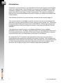
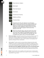
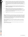
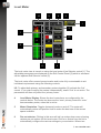
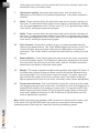
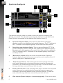
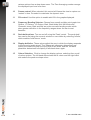
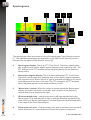
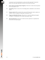
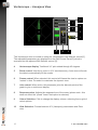
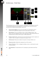
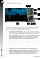
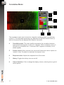
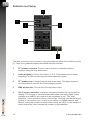
Operation Manual
Visualizer
Operation Manual
© 2014 NUGEN Audio
Contents
Page
Introduction
3
Interface Overview
4
Displays and controls
7
Level Meter
7
Spectrum Analysers
9
Spectrograms
11
Vectorscope
13
Lissajous
13
Polar
14
Correlation by Frequency
15
Correlation Meter
17
Statistics and Setup
18
An introduction to FFT analysis
19
Reporting a Problem
21
Version History
22
2
© 2014 NUGEN Audio
Introduction
Visualizer is a comprehensive, user definable real-time audio analysis tool designed
to give you rapid access to the information you need to fully understand your audio.
Visualizer is capable of providing a great deal of detailed information, coupled with
options that allow a high degree of user customisation. This manual is intended to
help both the novice and professional quickly navigate the interface and achieve the
results desired.
The manual is divided in to several sections, as listed on the contents page (2).
The overview section is intended to give the new user a broad run-through generic
operations such as selecting different views, opening control panels, etc. This section
is recommended reading for anyone new to the software, introducing concepts and
highlighting themes that run through the interface, improving workflow and intuitive
operation.
The displays and controls section is a detailed reference to every available
parameter view by view. Visualizer cannot be ‘broken’ by changing parameters and it
is recommended that the user refer to this section whilst using Visualizer in practice
so that the direct result of modifications can be seen in the displays.
An introduction to FFT analysis is also provided for those who are interested in
understanding how digital audio analysis works within Visualizer. The strengths and
weaknesses of this approach are discussed, which will allow the more advanced user
to make informed decisions, particularly with respect to the Set-up options, which
allow the user to adjust several of the underlying algorithmic parameters.
3
© 2014 NUGEN Audio
Interface Overview
The Visualizer interface is divided into three main sections. The graphical view
display area [1], the view selector controls [2] and the control panel [3]. The top edge
of the interface also contains several generic functions described below [4, 5 & 6].
5
6b
7
8
9
3
4
1
2
6a
1
Graphical View Display Area. This is where the results of the audio analysis
are displayed.
This area is treated as ‘soft space’ and can be configured to show a variety of
different views. This is a distinct advantage over many audio analysis tools,
which often require the user to select another interface module in order to
change the display, or even prohibit certain view combinations entirely.
Visualizer uses ‘intelligent window optimisation’ to reconfigure the displays,
changing size and positioning to allow the optimum view possible
automatically, without the user needing to juggle them around by hand.
2
View Selectors. This column of controls selects the various views available
for display. Clicking a control ‘on’ will cause the corresponding view to appear
in the graphical display area [1], clicking an active control will remove that view
from the display. The icons on the controls depict the view in question as
shown below.
Level Meter
Spectrum Analyser
4
© 2014 NUGEN Audio
Stereo Spectrum Analyser
Spectrogram
Stereo Spectrogram
Vectorscope
Correlation by Frequency
Statistics and Setup
Correlation Meter
Alongside most of the view selectors is an edit selector
control. These are used to select the controls available in the
Edit Control Panel [3]. Click the control adjacent to the View
Selector you wish to adjust and the Edit Control Panel will
display the controls available for adjusting that view. To hide
the Edit Control Panel all together, click the active Edit
Selector to turn it off.
Most of the views also have a view solo control. This control
can be used to fill the graphicsl display area [1] entirely with
the chosen view to allow an instant detailed inspection of the
chosen view. This control operates as an exclusive solo, and
is available even when a view is not currently displayed.
3
Edit Control Panel. The Edit Control Panel is where the various controls for
adjusting the different displays are shown and is accessed via the edit
selectors [2]. What is shown here will depend upon the active edit selector.
The panel can be hidden from view so as to maximise the available view
space by clicking the active edit selector.
4
Link control. The link control is a handy feature designed to allow rapid
changes to be made to multiple displays simultaneously. Simply put, when
‘Link’ is selected, the interface automatically updates ‘equivalent parameters’
for all views, including the one being adjusted on screen. E.g. If the link is
selected and a view is magnified using the zoom feature, all other views with a
like scale will also be magnified in the same way. If ‘Link’ is not selected, then
only the individual control being adjusted will be affected. Another example
would be using the link control to turn on/off all the peak hold views at once.
5
Clear. The clear button can be used to reset current views, removing peak
hold envelopes. This can be useful when a specific section of audio is being
inspected in a larger piece.
5
© 2014 NUGEN Audio
6
Resize. The Visualizer interface is fully resizeable via the bottom right-hand
corner [6a] (drag click to choose the aspect ratio and size desired). There are
also two size memories that can be toggled using the resize button [6b]. This
can be especially useful if screen real estate is at a premium, allowing a
'compact' display which can be immediately expanded for detailed inspection if
required.
7
Compare. The compare function allows two different audio streams to be
overlaid in the one interface for direct comparison and is described in it's own
section of the manual below.
8
Presets. Visualizer comes with a number of preset configurations. Most
Visualizer parameters can be stored with a preset, allowing rapid
reconfiguration for different tasks by recalling a previously stored setting. Use
the arrow controls to step up/down through the available presets, or click the
end control to bring up a preset menu.
9
Plugin Title. Click in this area to open the credits and licensing screen.
Zoom and Scroll. Several views within Visualizer are scaled (either in dB or against
frequency – or both). These views can be adjusted to show ranges in greater detail
by zooming and/or scrolling the scales. This is achieved by moving the mouse over
the scale in question and dragging along the line of the scale to scroll, and dragging
in a perpendicular direction to zoom in/out. To reset the scale to the full range hold
down control (Ctrl) and click the scale.
Numeric Windows. The numeric values indicated in Visualizer can be adjusted
either by click and dragging vertically, or double clicking and entering the desired
value directly.
Default values. Holding down control (Ctrl) and clicking a control will return the
control to the default position.
6
© 2014 NUGEN Audio
Level Meter
12
9
6
2
1
5
7
10
4
8
11
13
3
The level meter view is turned on using the level meter View Selector control [1]. The
adjustable parameters are displayed on the Edit Control Panel [3] which is accessed
via the adjacent Edit Selector control [2].
The level meter offers several pre-set scales and is also fully customisable to suit
individual requirements using the following controls.
NB: To adjust both primary and secondary meters together [4], activate the ’link’
control. If you wish to adjust the meters independently, ensure ‘link’ is not active. The
parameters will then only affect the ‘primary meter’.
4
Level Meter Display. Shows the level meter bars, as configured by the
controls below. The centre two bars are the ‘inner’ primary meter the ‘outer’
bars secondary meter, when this is active.
5
Meter Orientation. Toggles horizontal mode on and off. The meter will
automatically resize and position itself to make the best use of the screen
space available.
6
Pre-set selector. Clicking in this area will call up a drop-down menu showing
various pre-set options for the level meter. Click on a choice from the list to
automatically configure the various settings to your selection. Where two
7
© 2014 NUGEN Audio
meter-types are chosen, the first named will be the inner, primary meter, and
second the outer, secondary meter.
7
Appearance setting. Using this drop-down menu, you can select the
appearance of the meter to suit personal preference, or the audio material in
question.
8
Splits. These controls define the split points and colours for the 3 sections of
the meter. To understand these options more clearly try adjusting the settings
with the meter appearance set in ‘Sharp’ mode [7], if you get lost simply select
a pre-set [6]. and begin experimenting again.
9
Splits. These controls define the split points and colours for the 3 sections of
the meter. To understand these options more clearly try adjusting the settings
with the meter appearance set in ‘Sharp’ mode [7], if you get lost simply select
a pre-set [6]. and begin experimenting again.
10
Peak Controls. This section, outlined in grey, contains the parameters for
adjusting the peak-hold bar. The ‘Peak’ button toggles the function on/off. The
numeric window allows the peak hold time to be adjusted to suit personal
preference. The ‘infinite’ button overrides the peak hold time, setting it to hold
forever.
11
Meter ballistics. These values adjust the way in which the meter responds to
the incoming audio signal. The ‘Response’ parameter determines how quickly
the meter will jump up to the level of the audio, and the ‘fall-back’ parameter
determines how rapidly it falls back down again.
12
Margin. The margin indicates the dB remaining below true digital Full Scale. If
the audio clips (see the Setup and Stats module) this will be indicated with a
red warning light. Click in this area to reset the margin. The white, lager size
figure reflect the margin for the inner, primary meter, the smaller sized grey
figures represent the value for the outer, secondary meter (where appropriate).
13
Zoom and scroll zone. This is achieved by moving the mouse over the scale
and dragging along the line of the scale (vertically) to scroll, and dragging in a
perpendicular direction (horizontally) to zoom in/out. To reset the scale to the
default range hold down control (Ctrl) and click the scale. When zooming the
level meter, additional divisions at 1dB, 0.5dB and 0.1dB will show once the
scale is significantly expanded.
Note: RMS levels apply the standard –3dB correction so that pure sine waves read
at the same level on both RMS and Peak meters in accordance with hardware
mastering meters (Dorrough etc.) and the K-Metering mastering system.
8
© 2014 NUGEN Audio
Spectrum Analysers
6
8
7
10
9
11
2
1
12
4
13
7
5
8
3
15
14
The spectrum analyser views are turned on using the spectrum analyser View
Selector controls [1]. The adjustable parameters are displayed on the Edit Control
Panel [3] which is accessed via the adjacent Edit Selector control [2].
4
Spectrum Analyser display. This is an FFT (Fast Fourier Transform)
spectrum analysis view, graphing level against frequency. The FFT settings for
all FFT windows can be adjusted globally via the Stats and Setup control.
5
Stereo Spectrum Analyser display. This is a stereo-differential FFT (Fast
Fourier Transform) spectrum analysis view, graphing level against frequency.
Bias to the left is indicated above the centre ‘zero’ level and to the right below.
The FFT settings for all FFT windows can be adjusted globally via the Stats
and Setup control.
6
‘Mouse-over’ readout. When the mouse is moved around a Spectrum
Analyser display, the pointer becomes a cross-hair, and a readout of the X,Y
values at that point is displayed top right.
7
Zoom and scroll zone. Click and drag in this area to activate zoom and
scroll mode. Movement in a horizontal direction zooms the dB range and
movement in a vertical direction scrolls up and down. To reset the scale to the
full range hold down control (Ctrl) and click the scale.
8
Zoom and scroll zone. Click and drag in this area to activate zoom and scroll
mode. Movement in a vertical direction zooms the frequency range and
movement in a horizontal direction scrolls to the left and right. To reset the
scale to the full range hold down control (Ctrl) and click the scale.
9
View selector (Stereo Analyser – time averaging only). Click here to select
9
© 2014 NUGEN Audio
various options from a drop-down menu. The Time Averaging modes average
the displayed input level over time.
10
Freeze control. When selected, this control will freeze the view to capture an
‘instant’ in time. De-select to reactivate the dynamic view.
11
Fill control. Use this option to enable solid fill in the graphs displayed.
12
Frequency Banding Selector. Choose from smooth multiple point graph into
Octave, 1/3 Octave, 1/6 Octave, Bark, Bark thirds, Mel, Mel thirds and
Chromatic views. Bark and Mel are pycho-acoustic banding scales which
place greater definition in the frequency ranges where the ear is most
sensitive.
13
Peak-hold options. Turn on and off using the ‘Peak’ control. The peak-hold
time can be set using the numeric window or over-ridden by selecting ‘Infinite’,
which enables ‘hold forever’ mode.
14
Display ballistics. These values adjust the way in which the display responds
to the incoming audio signal. The ‘Response’ parameter determines how
quickly the meter will jump up to the level of the audio, and the ‘fall-back’
parameter determines how rapidly it falls back down again.
15
Colour Selection. Click to change the display colours, selecting from a grid
of colour options. The left hand side selects the fill colour and the right hand
side selects the peak envelope colour.
10
© 2014 NUGEN Audio
Spectrograms
7
11
8
9
2
10
4
12
1
5
3
8
7
6
13
The spectrogram views are turned on using the spectrogram View Selector controls
[1]. The adjustable parameters are displayed on the Edit Control Panel [3] which is
accessed via the adjacent Edit Selector control [2].
4
Spectrogram display. This is an FFT (Fast Fourier Transform) spectrogram
plot, graphing level (colour depth) against frequency with respect to time.. The
FFT settings for all FFT windows can be adjusted globally via the Stats and
Setup control.
5
Stereo Spectrogram display. This is a stereo-differential FFT (Fast Fourier
Transform) spectrogram plot, graphing level (colour depth) against frequency
with respect to time. Bias to the left or right is indicated according to the colour
scale displayed at the foot of the view. The FFT settings for all FFT windows
can be adjusted globally via the Stats and Setup control.
6
‘Mouse-over’ readout. When the mouse is moved around the Spectrogram
display, the pointer becomes a cross-hair, and a readout of the frequency
value at that point is displayed top right.
7
dB colour depth scale. Indicating the level in dB’s as represented by the
Spectrogram. Click and drag left or right to shift the dB bands represented by
each colour (not Stereo Spectrogram). Left and Right are indicated separately
in the case of the Stereo Spectrogram.
8
Zoom and scroll zone. Click and drag in this area to activate zoom and scroll
mode. Movement in a vertical direction zooms the frequency range and
11
© 2014 NUGEN Audio
movement in a horizontal direction scrolls to the left and right. To reset the
scale to the full range hold down control (Ctrl) and click the scale.
9
View selector (not Stereo Spectrogram). Click here to select various options
from a drop-down menu.
10
Smoothing. Select to smooth out the display data or deselect to view the raw
values.
11
Freeze control. When selected, this control will freeze the view to capture an
‘instant’ in time. De-select to reactivate the dynamic view.
12
Frequency Banding Selector. Choose from a smooth multiple point graph ,
or Octave, 1/3 Octave and 1/12 Octave (chromatic) views.
13
Spectrum Selector. Click here to select a colour spectrum to represent the
levels within the Spectrogram.
12
© 2014 NUGEN Audio
Vectorscope – Lissajous View
10
7
6
3
4
5
1
9
8
2
The Vectorscope view is turned on using the Vectorscope View Selector control [1].
The adjustable parameters are displayed on the Edit Control Panel [3] which is
accessed via the adjacent Edit Selector control [2].
4
Vectorscope display. Traditional X/Y plot rotated through 45 degrees.
5
Zoom control. Use this to zoom in (X/Y simultaneously). Auto zoom will scale
the data to automatically fill the screen.
6
Freeze control. When selected, this control will freeze the view to capture an
‘instant’ in time. De-select to reactivate the dynamic view.
7
Join control. When active, this parameter joins the discreet points of the
graph to give a continuous display.
8
Response value. Adjusts the response time of the meter (please note - this
does not effect the “joined” lines if that option is selected).
9
Colour Selection. Click to change the display colours, selecting from a grid of
colour options.
10
View Selection. Choose between X/Y (Lissajous) presentation and Polar
view.
13
© 2014 NUGEN Audio
Vectorscope – Polar View
10
7
6
3
4
1
5
9
8
2
The Vectorscope view is turned on using the Vectorscope View Selector control [1].
The adjustable parameters are displayed on the Edit Control Panel [3] which is
accessed via the adjacent Edit Selector control [2].
4
Vectorscope display. In this view, the rotated X/Y parameters used to
construct the traditional Lissajous view are presented in Polar form.
5
Stereometer. Gives an indication of the overall Left/Right balance. The
shorter, thin line responds quickly to the input signal, where as the thicker line
responds with an inbuilt inertia to give a wider perspective.
6
Freeze control. When selected, this control will freeze the view to capture an
‘instant’ in time. De-select to reactivate the dynamic view.
7
Solid control. Determines whether the polar envelope is filled or not.
8
Response value. Adjusts the response time of the meters.
9
Colour Selection. Click to change the display colours, selecting from a grid
of colour options.
10
View Selection. Choose between X/Y (Lissajous) presentation and Polar
view.
14
© 2014 NUGEN Audio
Correlation by Frequency
7
8
6
9
10
5
4
1
5
12
11
2
The correlation meter view is turned on using the correlation meter View Selector
control [1]. The adjustable parameters are displayed on the Edit Control Panel [3]
which is accessed via the adjacent Edit Selector control [2].
4
Correlation by Frequency display. This is an FFT (Fast Fourier Transform)
spectrum analysis view, graphing level against frequency. The FFT settings for
all FFT windows can be adjusted globally via the Stats and Setup control.
5
Zoom and scroll zone. Click and drag in this area to activate zoom and scroll
mode. Movement in a vertical direction zooms the frequency range and
movement in a horizontal direction scrolls to the left and right. To reset the
scale to the full range hold down control (Ctrl) and click the scale.
6
View selector. Click here to select between dynamic and time averaging
modes from a drop-down menu. The Time Averaging modes average the
displayed input over time.
7
Freeze control. When selected, this control will freeze the view to capture an
‘instant’ in time. De-select to reactivate the dynamic view.
8
Fill control. Use this option to enable solid fill in the graphs displayed.
9
Frequency Banding Selector. Choose from smooth multiple point graph into
Octave, 1/3 Octave, 1/6 Octave, Bark, Bark thirds, Mel, Mel thirds and
Chromatic views. Bark and Mel are pycho-acoustic banding scales which
place greater definition in the frequency ranges where the ear is most
15
© 2014 NUGEN Audio
sensitive.
10
Peak-hold options. Turn on and off using the ‘Peak’ control. The peak-hold
time can be set using the numeric window or over-ridden by selecting ‘Infinite’,
which enables ‘hold forever’ mode.
11
Display ballistics. These values adjust the way in which the display responds
to the incoming audio signal. The ‘Response’ parameter determines how
quickly the meter will jump up to the level of the audio, and the ‘fall-back’
parameter determines how rapidly it falls back down again.
12
Colour Selection. Click to change the display colours, selecting from a grid of
colour options. The left hand side selects the fill colour and the right hand side
selects the peak envelope colour.
16
© 2014 NUGEN Audio
Correlation Meter
7
6
5
3
4
5
1
8
2
The correlation meter view is turned on using the correlation meter View Selector
control [1]. The adjustable parameters are displayed on the Edit Control Panel [3]
which is accessed via the adjacent Edit Selector control [2].
4
Correlation meter. The meter position represents the correlation between
right and left-hand signals. A value of 1 indicates 100% correlation (mono), 0
indicated no correlation and –1 indicates 100% negative correlation (out of
phase signals).
5
Freeze control. When selected, this control will freeze the view to capture an
‘instant’ in time. De-select to reactivate the dynamic view.
6
Response value. Adjusts the response time of the meter.
7
History. Toggles the history view on and off.
8
Colour Selection. Click to change the display colours, selecting from a grid of
colour options.
17
© 2014 NUGEN Audio
Statistics and Setup
2
3
4
5
6
1
The stats and setup view is turned on using the stats and setup View Selector control
[1]. There is no graphical display associated with this selection.
2
FFT window selection. Choose from a selection of standard window
functions using the drop down menu.
3
Audio weighting. Choose from None, A, B, C, D standard equal loudness
weightings, or from various log-scale-linear spectrum slopes.
4
FFT window size. Choose from the drop down menu. The larger sizes are
recommended for use with the Time Averaging modes.
5
RMS window size. Choose form the drop down menu.
6
Clip Counter parameters. Visualizer constantly monitors the input signal for
clipping. The ‘number to clip’ parameter determines how many digital ‘overs’
(samples over 0dBFS) are required to be considered a ‘clip’. The ‘total’
parameter counts the total number of such clips. ‘Running’ records the largest
number of consecutive ‘over’ events in one section of clipped material, and
‘Blocks’ counts the number of events which qualify as a clip, i.e. the number of
events where the ‘overs’ exceed the number to clip parameter.
18
© 2014 NUGEN Audio
An introduction to FFT Analysis
This section is intended as a slightly more technical introduction to the world of FFT
analysis. It is not essential to understand the contents of this section to use
Visualizer, but a broad understanding of FFT analysis, and the trade-offs involved,
may help users appreciate some of the finer points.
Audio signals are represented as digital waveforms of signal value against time, so a
pure 1kHz tone signal is represented by a waveform, which rises and falls over time
in a sine-wave. However, this is not how the ear and brain perceive audio signals.
Our perception of audio is more to do with what frequencies are present in the signal,
and at what volumes, so, to give a useful visual representation of an audio signal, a
common approach is to try to display a graph showing the strength of any
frequencies in the signal.
Unfortunately, finding which frequencies are present in a signal is not a simple
matter. The mathematical process used to decompose a signal into its constituent
frequencies is known as the Fourier Transform. The simplest way of programming in
this transformation is so processor intensive that it cannot be used in real-time
applications. Thankfully, there is a well-known, much faster, way of implementing a
Fourier Transform, known as the Fast Fourier Transform (FFT), which does make
signal to frequency conversions possible in real-time.
Sample Rate:
Digital audio signals contain samples taken at a particular "sample-rate" (for example
44.1kHz). The higher the sample rate, the more disc space you need to store a given
length of audio, and the more processor power you need to manipulate it, but also,
the higher the frequencies you can store. Each sample rate has a maximum
frequency it can represent mathematically (called the Nyquist frequency), although it
could be argued that human perception of frequencies would start to degrade below
that absolute limit. As an example, a 44.1kHz audio signal, which was transformed by
an FFT, would not show any frequencies above 22.05kHz.
FFT Sample Size:
When an FFT is carried out on an audio signal, it is usually on separate chunks of the
signal, to give a reading of the frequencies present in each section of the audio. For
example, one could carry out an FFT on a 100ms section of audio to find out the
strengths of each frequency in that snippet. The number of samples in the chunk that
the FFT is applied to is called the "FFT sample size". There are trade-offs involved in
choosing the correct sample size to use. A small sample size will only contain a short
sample of audio data (for example a sample of 256 values from a 44.1kHz audio
signal will only be sampling over approximately 6ms), which means that it will be hard
for the FFT to accurately detect low frequencies (in our example, we are sampling
over 6ms, which corresponds to the wave-length of a signal near 170Hz, so we
couldn't expect any kind of accuracy for frequencies below this). Choosing a larger
sample size will give us more detail and accuracy in the lower frequency range,
however, as well as increasing the CPU loads slightly, this can lead to a lack of
responsiveness in the readings. As an example, if we are using a sample size of
16384 from a 44.1kHz audio signal, each chunk will be over approximately 350ms,
19
© 2014 NUGEN Audio
meaning that the frequency view will only be updated less than three times a second,
giving a rather sluggish feeling display.
FFT Window Function:
As FFTs are applied to limited sized chunks of an audio signal, they can only
approximate the frequencies, which are actually in that signal. Indeed, the
frequencies present in the signal might be changing over the period of that chunk.
By using different "windowing functions" the approximation of the FFT can be made
more precise in some ways at the expense of less accuracy in other ways. The main
trade off is of "frequency leakage" against "resolution". To illustrate the meaning of
these two terms consider an audio signal with a pure tone at 1kHz. In theory the
perfect frequency graph of this would have 0 at every frequency except at 1kHz,
where it would have a perfect spike up to the volume of that frequency. In reality, a
FFT graph from this signal will show a graph rising to a peak at 1kHz, and then
dropping off again. With better, that is less, frequency leakage, the regions of the
graph on the two sides of the peak would be lower (ie- less frequencies would be
leaking through where they shouldn't be). With better, that is higher, resolution, the
actual peak of the graph would be sharper. With a lower resolution, the peak of the
graph would be rounded, and flatter at the top. Higher resolution is more important
for distinguishing individual frequencies in a signal, lower leakage is more important
for signal which contain a lot of different frequencies. For audio signals, lower
leakage is usually more important, and so the default FFT window function in
Visualizer is chosen to have very low frequency leakage at the expense of some
resolution.
20
© 2014 NUGEN Audio
Reporting a problem.
If you encounter a problem with any of NUGEN Audio's products, please let us know,
to help us improve them.
Please email NUGEN Audio at [email protected] giving a clear
explanation of the problem. Please state how frequently you've experienced the
problem. If there are any particular steps you need to go through to see the problem,
please detail these.
Please also state your operating system, and the rough specs for your machine
(e.g.- CPU speed, RAM) - in Windows XP you can get this information by rightclicking "My Computer" and selecting properties.
Please be patient with any problems you may experience, particularly with products
at a beta stage of release. At NUGEN Audio we take problems with our software
seriously, and will endeavour to correct them as quickly as possible.
21
© 2014 NUGEN Audio
Version History
2.0
22
Initial release
© 2014 NUGEN Audio