1
Phone :
Fax :
Mail:
+49 (0)561 804 2654 / 2632
+49 (0)561 804 3631
[email protected]
Internet:
www.uni-kassel.de/fb14/leichtbau
ISSPA 02
Identification of Structural System Parameters
Version ISSPA02-03
User’s Guide
(extract)
Revision 19-January-2004
ISSPA02 User’s Guide
2
Table of Contents
1 ... ISSPA Installation
5
2 ... General
7
3 ... Theoretical Background
9
4 ... ISSPA Input Features
27
5 ... ISSPA Modules
5.1 ISPMOD
5.2 FITKOR
5.3 ISPKON
5.4 ISSPA
5.5 NOMOIS
5.6 DAMPF
5.7 ISPRES
5.8 FUELLEIS
5.9 ISPGEN
39
39
40
41
42
43
44
45
46
47
6 ... Using the ISSPA GUI
6.1 General
6.2 Getting started
49
49
62
7 ... ISSPA Main Results Files
83
8 ... Reference and Related Literature
85
ISSPA02 User’s Guide
Abbreviation
MDOF
UKL
GUI
FRF
measurement degree of freedom
University of Kassel, Department of Civil Engineering, Laboratory of
Lightweight Structures and Structural Mechanics
Identification of Structural System Parameters
high performance numeric computation and visualization software,
MATHWORKS
graphical user interface
frequency response function
x, y, z,
xx, yy, zz
MDOF direction
UX, UY, UZ
UXX, UYY, UZZ
translational MDOF
rotational MDOF
FX, FY, FZ
FXX, FYY, FZZ
nodal excitation forces
nodal excitation forces (moments)
n, N
r, MFG
nf
m
overall number of MDOF
overall number of modes
overall number of exciter forces
overall number of spectral lines, frequency points
Üb
base acceleration
{filename}
file not necessarily needed
ISSPA
MATLAB
3
ISSPA02 User’s Guide
4
ISSPA02 User’s Guide
1. ISSPA Installation
5
1. ISSPA Installation
The
software
package
ISSPA
comprises
FORTRAN
executables
and
MATHWORKS/MATLAB command Files (m-files). The FORTRAN executables are the
kernel of the identification procedure and may be called independently from any other
software using simple operating system commands. A graphical user interface (GUI) has
been provided to ease the application of the ISSPA modules and to produce all graphical
output. The GUI is implemented into MATHWORKS/MATLAB using several MATLAB
command files (*.m, or *.p). Therefore, ISSPA requires that MATHWORKS/MATLAB
Version 5.3 or higher is installed on the computer (PC or UNIX workstation) if the ISSPA
GUI is to be used.
ISSPA is distributed on a media using the following directory structure:
ISSPA
---------------------------------------------I-------------------------------------I
I
I
I
I
I
I
I
I
demo
docu
ein
exe
for
pcode
src
s2_unix
sgi_unix
contents:
demo
docu
ein
exe
for
pcode
src
s2_unix
sgi_unix
ISSPA demo identification (ref. Appendix E )
ISSPA documentation (Microsoft WORD 97 documents or pdf documents)
Templates of ISSPA input files
ISSPA FORTRAN executables
ISSPA FORTRAN sources
ISSPA graphical user interface (p-code)
ISSPA graphical user interface
ISSPA implementation tools for SUN/SOLARIS 2
ISSPA implementation tools for SILICON-GRAPHICS
In addition the media includes the ukl\tbox , a special software package which includes
general data handle tools which are commonly used by several UKL software packages.
To run ISSPA within MATLAB the MATLABPATH has to be extended to include the
following directories:
• ukl\isspa\src or ukl\isspa\pcode\matlab*
• ukl\tbox
Note:
If only the pcode edition or the limited edition of ISSPA is available the user must link the
corresponding subdirectory matlab51, ..., matlab65 of the \pcode directory to the
MATLABPATH.
The user must also set the operating system program search path to include ukl\isspa\exe and
ukl\tbox. Refer to the User's Manual of your computer to properly set the program search
path.
Note:
ISSPA02 User’s Guide
1. ISSPA Installation
6
Your implementation of ISSPA may differ from this general directory structure due to
individual requirements.
To check the ISSPA installation it is recommend to copy the demo directory to a temporary
working directory and start the auto sequence of demonstration examples by calling demo_all
within MATLAB from the actual demo directory.
ISSPA02 User’s Guide
2. General
7
2. General
ISSPA is a software package for the identification of linear structural system parameters. It is
developed by the 'Department of Lightweight Structures and Structural Mechanics' at the
'Department of Civil Engineering' at the 'University of Kassel, Germany' (UKL), Prof. Dr.
Ing. M. Link. ISSPA comprises standalone FORTRAN executables and a graphical user
interface (GUI) written using MATHWORKS/MATLAB /10/ computation and visualization
software. ISSPA is aimed to be used to solve low to medium scaled problems up approx. 800
measurement degrees of freedom (MDOF) and 3200 spectral lines. The developers of ISSPA
put much more emphasis on the solution algorithms and the variety of applications than on
graphical user interface programming. Due to this, the user has to take a high share on
specifying all needed input data correctly.
ISSPA expects the user to be a so called ‘friendly user’, i.e.
- he/she has a basic knowledge in mechanics and structural identification to supply the
needed input data and interpret the output results
- he/she has a basic knowledge in using MATHWORKS/MATLAB
ISSPA is certainly not designed for users who want to proof how stupid software can be. Nor
should the user be disappointed, if the application may fail due to erroneous input.
The software package ISSPA (Identification of Structural System Parameters) consists of
nine modules :
ISPMOD
Selection of identification frequency ranges
FITKOR
Curve fit identification of modal parameters and residual correction
ISPKON
Condensation of measurement matrices to effective degrees of freedom
-> modified measurement
ISSPA
Identification of modal parameters from modified measurement
NOMOIS
Assembly of the inverse physical system matrices
DAMPF
Damping matrix improvement using a modal approach
ISPRES
Recalculation using identified data
FUELLEIS
Assembly of the results of different frequency ranges
ISPGEN
Calculation of dynamic responses from given modal data
The theory on which the software package is based is described in /1/,/2/,/3/,/13/,/18/. A
comprehensive introduction to the theory is given in chap. 3 of this manual.
ISSPA02 User’s Guide
2. General
8
The ISSPA software package comprises two different identification procedures :
FITKOR
an identification approach based on modal parameters
ISSPA
an identification approach based on physical parameters
Both procedures share a common data basis. This data basis consists of several data files and
an internal program control file. These files manage the data transfer between the modules
and are generally not used or modified by the user.
To perform a FITKOR identification the following modules are used successively
ISPMOD
data preprocessing
FITKOR
identification using a simplified modal approach, residual correction
ISPRES
recalculation using identified data
To perform an ISSPA identification the following modules are used successively
ISPMOD
data preprocessing
FITKOR
residual correction
ISPKON
condensation of measurement matrices
ISSPA
identification using a physical approach
NOMOIS
assembly of inverse system matrices
DAMPF
damping matrix improvement, if required
ISPRES
recalculation using identified data
Note: if no residual correction is required FITKOR can be skipped
All control input to a module is given in a ASCII input file with a fixed filename. This
filename consists of the module name and the extension *.ein, e.g. ISPMOD.EIN. All input
files (except ISPGEN.EIN) are specified using the UKL *.FR3 file specifications which is
given in appendix A. Templates of the input files are given in appendix B and in the ein
directory.
Each module creates a ASCII file which lists input data, program flow and results. The
filename is fixed and consists of the module name and the extension *.aus, e.g.
ISPMOD.AUS.
In order to manage the internal data flow between the modules unformatted and formatted
sequential files are created. A list of these files is given in appendix C. The files follow the
UKL *.FR3, *.UR3 file specifications. They have no further relevance to the user and should
be deleted after the results of an identification range are excepted. The ISSPA GUI provides
the Purge button to properly perform this task.
In practical applications the identification of a complete measurement data set is not
performed in a single step. Usually the overall data set is divided into several identification
ranges which are identified one by one. It is recommended to use a separate directory for each
identification range e.g. b001, b002, ... . When the identification of each separate
identification range is complete the modal parameters can be combined to an overall
identification results file using the ISSPA module FUELLEIS. This combination should also
be performed in a separate directory, e.g. bcmb . The ISSPA GUI provides on the ISSPA
START and ISSPA COMBINE windows basic tools to properly perform these data
management tasks.
ISSPA02 User’s Guide
3. Theoretical Background
9
3. Theoretical Background
Note:
The ISSPA User's Guide (extract) does not comprise chapter 3 of the original ISSPA User's
Guide.
For detailed information about the ISSPA theory refer to:
[a]
Link, M.:
Theory of a Method for Identifying Incomplete Matrices from Vibration Test Data,
Z. d. Flugwissenschaft und Weltraumforschung (ZFW) 9, 1985, Heft 2, 3
[b]
Krätzig, Meskouris, Link:
Baudynamik und Systemidentifikation
in: Der Ingenieurbau: Grundwissen,
Band 5, Baustatik, Baudynamik, (Mehlhorn Hrsg.)
Berlin 1995, Ernst & Sohn, ISBN 3-433-01571-6
[c]
Link, M.; Qian, G.:
Identification of Dynamic Models for Substructure Synthesis Using Base Excitation
and Measured Reaction Forces.
Revue Francaise de Mecanique, No. 1 (1994)
[d]
Kasai T. and Link M.: Identification of Non-Proportional Modal Damping Matrix and
Real Normal Modes. Mech. Systems & Signal processing, Vol. 16, No 6, 921- 934,
(2002)
ISSPA02 User’s Guide
4. ISSPA Input Features
27
4. ISSPA Input Features
The ISSPA identification procedure is based on the linear equation of motion in the frequency
domain. Therefore the basic ISSPA input features can best be explained by the frequency
response relation
( jω) = H ( jω)F( jω)
U
(n ,1)
(4.01)
(n , n f ) (n f ,1)
where
n = no. of measured degrees of freedom (MDOF)
nf = no. of exciter forces (nf ≤ n)
ω = excitation frequency
j= − 1 imaginary unit
(
H = − ω2 − ω2 M + K + jωD
( n ,n f )
)
−1
(4.02)
= nf columns of matrix of frequency response functions (inertance) w.r. to the
complex exciter force vector F = [F1 ... Fk ... Fnf]T
M, K, D = physical mass, stiffness and damping matrix
U = [U1 ... U n ]T
measured complex frequency acceleration response at n MDOF
The user must supply measured frequency acceleration response
( )
( jω)
U
and forcing
function F jω as input to the identification procedure. The type and amount of input
depends on the type of the identification problem. Refer to app. A-C for detailed input and
output file specifications.
ISSPA02 User’s Guide
4. ISSPA Input Features
28
Case I :
Constant harmonic (sinusoidal) force excitation with nf exciter forces
( ISSPA control parameters IHARMO = 1, IFUSS = 0)
Input
a) force vector F = [ F1 ... Fk ... Fnf ]T
real part
Fre = F = const. for all excitation frequencies ω
imaginary part Fim = 0
b) response Ü(jω) (equivalent to H(jω) F )
Output
a) eigenfrequencies, eigenvectors, modal masses, modal damping factors
b) inverse physical stiffness and mass matrix (incomplete)
Special case
FRF data provided by a standard data acquisition unit using e.g. a single shaker or a modal
impulse hammer:
Single point excitation at MDOF k with force Fk = 1. In this case the response is equivalent
to the k-th column of the frequency response functions (FRF matrix):
Ü(jω) = Hk(jω)
Note
If more than one exciter configuration was used for testing (like in classical modal survey
testing with force appropriation) the test data must be analyzed separately for each
configuration.
ISSPA02 User’s Guide
4. ISSPA Input Features
29
Case II :
Harmonic constant single axis base acceleration
( Data preparation outside ISSPA necessary, case II is thereby reduced to case I)
ISSPA control parameters IHARMO = 1, IFUSS =0)
It is assumed that the following basic data is available (ref. fig. 4.1):
• the measured acceleration frequency response of N degrees of freedom (MDOFs) well
distributed on the structure to gain a sufficient spatial resolution. The responses are
measured at m frequency points (spectral lines).
• the measured acceleration frequency response of the pilot accelerometers mounted on the
rigid interface shaker/structure.
• if available: measured reaction forces (i.e. measured by a force measurement device
/15,/17/)
• if available: the mass matrix of a FE model reduced to N MDOFs
Fig 4.1: Typical test configuration used in base excitation testing
ISSPA02 User’s Guide
4. ISSPA Input Features
30
There are three basic steps necessary to prepare the measured data from a sine base excitation
test for the ISSPA identification procedure
1. Calculation of the base excitation at reference (A) from the pilot pickups
2 Calculation of the relative response at the structural MDOFs with respect to the base
(A)
3 Definition of excitation forces
Note: All steps must be performed outside ISSPA, prior to an ISSPA identification.
1. Calculation of the base excitation at reference (A) from the pilot pickups
In base excitation testing, there are a number of pilot pickups mounted on the shaker table.
During test they are used as a part of the shaker control system. For the subsequent
identification process they provide all necessary information to calculate the applied base
excitation with respect to the mounting point of the test structure (point (A) in figs 4.1 and
4.2).
If the adapter and shaker table is rigid the relation between the pilot responses U
the base excitation U
A
(ω) is given for each excitation frequency ω by
⎡ uA
⎤
x
:
⎡ ⎤ ⎡. . .
.
.
. ⎤⎢ A
⎥
u
⎢u p ⎥ ⎢
0
z íp − y ip ⎥ ⎢ Ay ⎥
⎢ x i ⎥ ⎢1 0 0
⎥⎢ u ⎥
p
z
⎢ u p ⎥ = ⎢0 1 0 − z p
0
x
i
i ⎥⎢ A ⎥
yi
⎢ p ⎥ ⎢
⎥ ⎢u ⎥
p
− x ip
0 ⎥ ⎢ xx
⎢ u z ⎥ ⎢0 0 1 y i
u Ayy ⎥
⎢ i ⎥ ⎢. . .
⎥
. ⎦⎢ A ⎥
: ⎦ ⎣. . ⎣
⎢u ⎥
⎣
zz ⎦
p
p
T
U
p
(ω) and
(4.1)
UA
where
u px
i
response of the i-th pilot measured in x- direction
x ip , y ip , z ip distance of the i-th pilot location and reference (A)
uA
x
i
excitation at reference (A) in x- direction
number of pilot pickup i = 1,2,...np
Since the number of pilot DOFs can be much larger than the number of excitation DOFs the
pseudo inversion
+
U A = Tp U p
(4.2)
ISSPA02 User’s Guide
4. ISSPA Input Features
31
where
Tp
+
pseudo inverse of T
relates the base excitation U
A
p
p
and the measured pilot responses U in a least squares sense.
Example:
Determination of base excitation in X/Z- plane at reference (A) from 4 pilot MDOFs
Fig 4.2: Base excitation in X/Z plane
Eq. (4.1) yields
⎡up ⎤ 1 − α b
⎤
⎢ xp1 ⎥ ⎡
⎤
⎢ u z 1 ⎥ ⎢0
b ⎥⎡ u A
x
⎥
⎢
=
⎢
⎢ p ⎥
A ⎥
⎥
⎢
−
α
1
b
u
u
⎢
⎢ x2 ⎥
⎣ yy ⎥⎦
⎥
⎢
⎢ u p ⎥ ⎣0 − b ⎦
⎣ z 2 ⎦ (4.3)
Tp
The pseudo inverse of T
p
is given by
+
T
T p = ⎛⎜ T p T p ⎞⎟
⎠
⎝
−1
Tp
T
(4.4)
ISSPA02 User’s Guide
4. ISSPA Input Features
32
From that, the base excitation at reference (A) can be calculated
U Ayy
(
) (
)
1 p
U x1 + U px 2 + α U pz1 − U pz 2
2
1
= U pz1 − U pz 2
b
UA
x =
(
)
(4.5a)
(4.5b)
In the special case when the base rotations can be neglected
A
A
UA
xx = U yy = U zz ≈ 0
(4.6)
eq. (4.2) yields
UA
x =
U Ay =
UA
z =
1
n px
1
n py
1
n pz
∑U
p
xi
∑U
p
yi
∑U
p
zi
(4.7a-c)
where
n px , n py , n pz
overall number of pilots in X,Y,Z
In this case the base excitation in X,Y,Z is calculated from the average of the corresponding
pilots.
Note:
The actual software implementation of ISSPA requires a constant base excitation level
U A (ω) with respect to the excitation frequencies ω . Therefore U p (ω) should be constant
within the selected frequency range, i.e. only tests without notching should be used. However,
if only data from tests are available where input notching was applied the response of the
structural MDOFs U must be related to the base excitation by
ISSPA02 User’s Guide
4. ISSPA Input Features
⎡ U1x ⎤
⎢
⎥
U
⎢ 1y ⎥
⎢U ⎥
⎢ 1z ⎥
⎢ U 2x ⎥
⎢
⎥ =
:
⎢
⎥
⎢ : ⎥
⎢
⎥
U
⎢ Ny ⎥
⎢U ⎥
Nz ⎦
⎣
⎡
⎢
⎢
⎢
⎢
⎢
⎢
⎢
⎢
⎢
⎢
⎢
N⎣
33
⎤
⎥
⎥
⎥
⎥
⎥
⎥
⎥
⎥
⎥
⎥
⎦⎥
H
6
⎡ UA
⎤
x
⎢ A⎥
⎢ Uy ⎥
⎢ UA ⎥
⎢ Az ⎥
⎢ U xx ⎥
⎢U A ⎥
⎢ yy ⎥
⎢⎣ U A
⎥
zz
⎦
(4.8)
UA
U
The transfer function matrix H(ω) contains all structural information and therefore can be
used for modal identification. It can be calculated from
H = U UA
+
(4.9)
where
UA
+
pseudo inverse of U
A
In the general case of a base excitation in 3-D space six independent data sets (test runs) are
required to calculate U
excitation ( e.g.
A+
. However, if the base excitation can be considered as a single axis
A
U zA ≠ 0, U Ax = U Ay = U Axx = U Ayy = U zz
= 0 ) a column of the
transfer function matrix can be calculated simply from the complex division of the structural
MDOFs by the corresponding base excitation, e.g.
H (*, A
z
) (ω j )
=
( )
UA
z (ω j )
U ωj
(4.10)
where
H (*, A
j
z)
column of H with respect to a base excitation in Z direction at reference A
number of frequency point
j = 1,2,...,m
This column represents the response of the structure with respect to a unit single axis base
excitation (e.g. in Z). Hence, all structural MDOFs which direction coincide with the base
excitation direction must exhibit a transfer function of 1 in the low frequency range ( 0< ω <
first elastic structural mode). This is due to the rigid body movement of the structure in this
frequency range.
In the most practical case where a pure single axis base excitation is not achieved eq.(4.10)
yields the transfer functions with respect to a non fixed base. In this case all other base
excitation DOFs are treated as structural DOFs.
ISSPA02 User’s Guide
4. ISSPA Input Features
34
2. Calculation of the relative response at the structural MDOFs with respect to the base
(A)
In the case of the transfer function matrix (eq. 4.9-10) the rigid body part must be removed
from the transfer functions.
real
H real
− TH
rel = H
(4.11a-b)
imag
H imag
rel = H
where
imag
H real
rel , H rel
real, imaginary part of H with respect to the base A
TH
rigid body transformation matrix relating the unit base displacements
in excitation direction and the structural MDOFs responses
This modification effects only the real part and depends on the orientation of the structural
MDOFs with respect to the XYZ coordinate system defined by the base DOFs. So in the case
e.g. that the direction of a structural MDOF coincides with the base excitation direction the
value 1 must be subtracted from the real part of the transfer function.
In the more general case the relative response of a structural MDOFs is given by
U rel = U abs − T s U A
(4.12)
where
U rel
relative response
U abs
measured response
Ts
rigid body transformation matrix
.
.
. ⎤
⎡. . .
⎢1 0 0
0
z si
− y si ⎥ i - th MDOF in X
⎥
⎢
s
s
s
⎢
0
1
0
z
0
x
−
T =
i ⎥ i - th MDOF in Y
i
⎥
⎢
s
s
0 ⎥ i - th MDOF in Z
⎢0 0 1 y i − x i
⎢⎣ . . .
.
.
. ⎥
⎦
Ts
x si , y si , z si
distance of i-th structural MDOF to reference (A)
(4.13)
ISSPA02 User’s Guide
4. ISSPA Input Features
35
Example:
Calculation of the relative response of the first structural MDOF in X direction
abs
A
s A
s A
U rel
x1 = U x1 − U x − z1 U yy + y1 U zz
(4.14)
In the case that the base rotations can be neglected eq. 4.12 yields
abs
A
U rel
xi = Uxi − Ux
abs
A
U rel
yi = U yi − U y
(4.15)
abs
A
U rel
zi = Uzi − Uz
Note:
Either the transfer functions H rel or the relative displacements U rel are used for ISSPA
input.
3. Definition of excitation forces
To identify the modal masses in addition to the eigenfrequencies, mode shapes, modal
damping factors the excitation forces must be known. If a special force measurement device
at the junction shaker/structure is used they can be measured directly /15/, /17/. If an
analytical mass matrix with respect to the structural MDOFs is available, an equivalent
excitation force can be calculated for each MDOF using the reference excitation (A). In both
cases all modal parameters can be calculated. However, if the excitation forces are unknown,
all modal parameters except the modal mass can be calculated from the measured data.
a) excitation forces are unknown i.e. the interface reaction forces are not measured
In this case a dummy unit force F = 1 is applied at an arbitrary MDOF. However, the
identified modal masses have no physical meaning and are just needed to scale the
response in a recalculation (synthesized response using the identified data)
ISSPA02 User’s Guide
4. ISSPA Input Features
36
b) excitation forces are calculated from an analytical mass matrix
In this case an analytical mass matrix with respect to the N structural MDOFs must be
available. However, this mass matrix must represent sufficiently the inertia properties of
the structure.
The excitation forces are calculated by
F = −M T s U
A
(4.16)
where
M
F
analytical mass matrix with respect to the MDOFs
excitation force vector
T s rigid body transformation matrix acc. eq. (4.13)
Example:
The excitation forces for the structural MDOFs in X,Y and Z at the first measurement
point with an analytical lumped mass m1 at that point are calculated from
(
)
s A
Ay − z1s U
A
Fy1 = −m1 (U
xx + x1 U zz )
s A
s A
A
Fz1 = −m1 (U
z + y1 U xx − x1 U zz )
s A
s A
A
Fx1 = − m1 U
x + z1 U yy − y1 U zz
(4.17a-c)
ISSPA02 User’s Guide
4. ISSPA Input Features
37
After data preparation of the raw base excitation test data ISSPA can be applied to identify
the modal parameters
( ISSPA control parameters IHARMO = 1, IFUSS = 0)
Input
a1) force vector
F = −M T s U
A
or
a2) if analytical mass matrix M is not available:
F = 1 dummy unit force applied at an arbitrary MDOF
b) relative response with respect to the base
rel
U
A
Output
a) eigenfrequencies, eigenvectors, modal damping factors
if a1) is available : modal masses
Special case
Reference
Link M.; Ulrich H.; Weiland M.:
ISSPA Guidelines, Modal Identification using Base Excitation Test Data
Laboratory of Lightweight Structures and Structural Mechanics (UKL)
Kassel, April 1999
ISSPA02 User’s Guide
4. ISSPA Input Features
38
ISSPA02 User’s Guide
5. ISSPA Modules
5. ISSPA Modules
5.1: ISPMOD
Purpose
Selection of identification frequency ranges
Input of ISSPA control parameters to specify the type of identification
Input
ispmod.ein
Output
ispmod.aus
ispmod_01.mat
ispmod_02.mat
ISSPA control parameters
Measurement data file specification
supported formats:
UKL FR3 (app. A)
UKL UR3 (app. A)
UKL IDX (app. A)
MATLAB mat file (app.A)
SDRC Universal files, Type 58
max. filename length:132 characters
listing file
plot file
mode indicators
Limitations
dynamic allocation of matrix dimensions limited to overall 5.2 Million REAL*4 values
low to medium scaled problems e.g. N= 800 MDOF m= 3200 spectral lines, but
N*m < 2560000 (!)
Position in ISSPA sequence
post:
none
pre:
FITKOR
ISPKON
39
ISSPA02 User’s Guide
5. ISSPA Modules
5.2: FITKOR
Purpose
Curve fit identification of modal parameters and residual correction:
eigenfrequencies, eigenvectors, modal masses, diagonal modal damping matrix
Input
fitkor.ein
Output
fitkor.aus
fitkor_01.mat
FITKOR control parameters
eigenfrequency iteration limit ITFMAX
damping iteration limits ITDMAX
Iteration start values: eigenfrequencies, modal damping factors
listing file
plot file
residual corrected response
Limitations
identification using a simplified modal approach: diagonal damping matrix (proportional
damping)
Position in ISSPA sequence
post:
ISPMOD
pre:
ISPRES
ISPKON
40
ISSPA02 User’s Guide
5. ISSPA Modules
41
3.3: ISPKON
Purpose
Singular value decomposition of the measurement matrices to determine the number r of
effective modes in the identification range (rank of measurement matrices)
Condensation of measurement matrices to r effective degrees of freedom.
Input
{ ispkon.ein }
ISPKON control parameters
or interactively
no. of effective modes
Output
ispkon.aus
ispkon_01.mat
listing file
plot file
modified measurement
Limitations
Position in ISSPA sequence
post:
FITKOR
ISPMOD( if no residual correction is required)
pre:
ISSPA
ISSPA02 User’s Guide
5. ISSPA Modules
3.4: ISSPA
Purpose
Identification of modal parameters from modified measurement matrices:
eigenfrequencies, eigenvectors, modal masses, non-diagonal modal damping matrix
Input
Output
isspa.aus
listing file
Limitations
Position in ISSPA sequence
post: ISPKON
pre:
NOMOIS
42
ISSPA02 User’s Guide
5. ISSPA Modules
3.5: NOMOIS
Purpose
Assembly of the inverse stiffness and mass matrices
Deletion of noise modes
Input
{ nomois.ein }
NOMOIS control parameters
or interactively
no. of ISSPA mode shapes to be deleted
Output
nomois.aus
listing file
Limitations
Position in ISSPA sequence
post:
ISSPA
pre:
ISPRES
DAMPF
43
ISSPA02 User’s Guide
5. ISSPA Modules
3.6: DAMPF
Purpose
Damping matrix improvement using a modal approach
Input
{ dampf.ein }
DAMPF control parameters
or interactively
no. of spectral lines left/right to eigenfrequency to use for improving
the modal damping matrix
Output
dampf.aus
listing file
Limitations
Position in ISSPA sequence
post:
NOMOIS
pre:
ISPRES
44
ISSPA02 User’s Guide
5. ISSPA Modules
3.7: ISPRES
Purpose
Recalculation using identified data
Input
{ ispres.ein }
ISPRES control parameters
or interactively
no. of modes to be suppressed in the calculation
include residual effects, if previously calculated by FITKOR
Output
ispres.aus
ispres_01.mat
listing file
recalculated response
Limitations
Position in ISSPA sequence
post:
FITKOR
NOMOIS
pre:
45
ISSPA02 User’s Guide
5. ISSPA Modules
3.8: FUELLEIS
Purpose
Assembly of identification results of different identification ranges
Input
fuelleis.ein
FUELLEIS control parameters
Output
fuelleis.aus
fuel.fr3
listing file
modal parameters and inverse system matrices
Limitations
Position in ISSPA sequence
post:
FITKOR
of single identification ranges
NOMOIS " "
"
"
pre:
ISPRES
of combined identification range
46
ISSPA02 User’s Guide
5. ISSPA Modules
3.9: ISPGEN
Purpose
Calculation of dynamic responses from given modal data
Input
ispgen.ein
Output
ispgen.aus
isspa2is.ein
ISPGEN control parameters
modal parameters, dynamic response
listing file
ISSPA data file
Limitations
Position in ISSPA sequence
post
pre:
47
ISSPA02 User’s Guide
5. ISSPA Modules
48
ISSPA02 User’s Guide
6. Using the ISSPA GUI
49
6. Using the ISSPA GUI
6. 1 General
A graphical user interface (ISSPA GUI) has been provided to ease the application of the
ISSPA modules and to produce all graphical output. The GUI is implemented into
MATHWORKS/MATLAB using several MATLAB command files (*.m, or *.p). Therefore,
ISSPA requires that MATHWORKS/MATLAB Version 5.3 or higher is installed on the
computer (PC or UNIX workstation) if the ISSPA GUI is to be used.
To run the ISSPA GUI within MATLAB the MATLABPATH has to be extended to include
the UKL\ISSPA\SRC or UKL\ISSPA\PCODE\MATLAB* and the UKL\ISSPA\TBOX
directories, ref chap. 1. After MATLAB start the actual setting of the MATLABPATH can be
checked at any time by pressing path . The user must also set the operating system program
search path to include UKL\ISSPA\EXE and UKL\TBOX. Refer to the User's Manual of your
computer to properly set the program search path.
The ISSPA GUI is started by pressing isspa on the MATLAB command window .
After pressing isspa the ISSPA Plot window and the ISSPA Main window become visible
first. From these windows all other ISSPA windows and all ISSPA commands are accessible
using the respective pulldown menus or buttons. To exit ISSPA use the Mange pulldown
menu of an ISSPA window.
The ISSPA GUI consists of several subroutines, which are called from the ISSPA windows.
Almost all variables used in the ISSPA GUI are local variables which will be cleared after an
ISSPA task has been performed, so that the user has no access to any of these variables. The
ISSPA GUI also uses a set of global variables which are set when the ISSPA start command
isspa is pressed and cleared after the ISSPA exit command is executed. These global variables
are of no further relevance to the user. You can list these variables by pressing whos global on
the Matlab Command window after ISSPA was started.
The Matlab Command window is available at any time so that the user may perform other
calculations within MATLAB (e.g. MATFEM) while the ISSPA windows are active.
All data and identification results are stored in data files, which are written in the UKL FR3
format or the MATLAB mat file format (level 1, compatible to MATLAB Version 4 and 5).
Refer to app. A, C for a detailed listing of the file format and index. The user can read from
these data files by using the readfr3 command e.g.
read eigenvalues (real, imaginary part) and right and left hand eigenvectors
from the ISSPA data file nomo12.fr3
[lam_re, lam_im, Y, X]= readfr3( 'nomo12.fr3')
Press help readfr3 for detailed information about the input/output arguments of this
MATLAB call.
ISSPA02 User’s Guide
6. Using the ISSPA GUI
50
Data from MATLAB mat files can be loaded using the load command, e.g.
load measurement data of the actual identification range
load ispmod01
Refer to the MATLAB User's Guide or press help load for detailed information about the load
command.
There are several ISSPA pulldown menus available in the ISSPA windows which main
contents are listed below:
ISSPA Pulldown Menus:
Manage:
Select Working Directory
Exit ISSPA
Plot:
Close Figure
Keep Figure
keep actual ISSPA plot as separate figure
Menubar
on/off MATLAB Menubar
Select, Zoom
Zoom frequency axis graphically
Zoom off
Select MDOF
MDOF_SET_1
user defined MDOF set
MDOF_SET_2
MDOF_SET_3
all MDOF
Scan MDOF
Display MDOF one by one
Scales, View
Real/Imaginary
Amplitude/Phase
Nyquist
Waterfall
Waterfall of abs( Uim)
Parameter
log x
log y
log z
Rotate
rotate subplot graphically
all subplot
display all subplots of actual figure
upper subplot only
lower subplot only
ISSPA02 User’s Guide
6. Using the ISSPA GUI
ISSPA:
Select all available frequencies
Select identification ranges
- data reduction
Pick eigenfrequencies
ISSPA Control
Run FITKOR
Run ISSPALL
Run DAMPF
Run ISPRES
EF Blowup
specify identification range
perform automatic data reduction
view ISSPA Control window
Mode shape animation using a MATFEM FE model
(Only, if UKL\MATFEM is installed)
Tag:
Tag estimated eigenfrequencies
Tag identified eigenfrequencies
Window:
ISSPA Main
ISSPA Start
ISSPA Tools
ISSPA Control
ISSPA Linear Identification
ISSPA Nonlinear Identification
ISSPA Combine
ISSPA Plot
ISSPA Identification Process
ISSPA Identification Results
view ISSPA window
not activated in the actual ISSPA version
Print:
b/w Printer
b/w Paste
b/w *.bmp
Paste
*.ps
*.bmp
black/white plot to printer
black/white plot to paste buffer
black/white plot to bitmap file
plot to paste buffer
Post script file
Bitmap file
Help:
About
UKL Logo
51
ISSPA02 User’s Guide
6. Using the ISSPA GUI
52
Generally, there are 9 ISSPA windows which will be used in an identification process:
ISSPA Main
ISSPA Start
ISSPA Tools
ISSPA Control
ISSPA Linear Identification
ISSPA Combine
ISSPA Plot
ISSPA Identification Process
ISSPA Identification Results
The first six windows are used to control the identification run, whereas the later three are
used to present the identification results or to log the identification process. To switch among
those windows each window provides the pulldown menu Window. In addition, the upper six
windows provide buttons in the lower part of the window to easily switch to a different
window. If a certain window consists of several subwindows (e.g. ISSPA Linear
Identification) additional buttons are also provided in the lower part of the window to switch
the subwindows. The user may close or resize and reposition a window at any time. The
upper six windows provide a close button to close the respective window.
ISSPA Release
Buttons:
Select Working Directory
Fig. 6.1.1: ISSPA Plot window
ISSPA02 User’s Guide
6. Using the ISSPA GUI
53
Buttons:
main, start, tools, ctr
lin, cmb,
plot, id-log, list
close
Working Directory
Fig. 6.1.2: ISSPA Main window
Switch ISSPA window
close ISSPA Main window
Select working directory
ISSPA02 User’s Guide
6. Using the ISSPA GUI
54
Buttons:
create ispmod.ein
create fitkor.ein
create ISSPA subdirs
Create/Modify ispmod.ein
Create/Modify fitkor.ein
Create ISSPA identification
subdirectories b001...b050 and the
directory bcmb to combine
identification results from
identification subdirectories
main, start, tools, ctr
lin, cmb,
plot, id-log, list
Switch ISSPA window
Fig. 6.1.3: ISSPA Start window
ISSPA02 User’s Guide
6. Using the ISSPA GUI
55
Buttons:
unv->ur3
unv->mat
formum
main, start, tools, ctr
lin, cmb,
plot, id-log, list
Fig. 6.1.4: ISSPA Tools window
Convert Universal File Type 58 to
UKL UR3 File
Convert Universal File Type 58 to
MATLAB mat File
Convert UKL data files:
unformatted ⇔ formatted
Switch ISSPA window
ISSPA02 User’s Guide
6. Using the ISSPA GUI
56
Buttons:
close
ISSPA exe control:
DOS Window
messages
IDISP
AUTORUN :
ISPMOD
FITKOR
Close ISSPA Control window
Display channel of run time
during an ISSPA module run
Switch to control the amount of run
time messages during an ISSPA
module run
Start ISPMOD and plot data, if
ISPMOD called from ISSPA
pulldown menu
Start FITKOR after 'Pick
Eigenfrequencies' was called from
ISSPA pulldown menu
AUTOPLOT :
ISPMOD
FITKOR
Plot after termination of module
- measured response
- comparison of measured and
recalculated response
ISSPA XL
--- for development use only ---
main, start, tools, ctr
lin, cmb,
plot, id-log, list
Switch ISSPA window
Fig. 6.1.5: ISSPA Control window
ISSPA02 User’s Guide
6. Using the ISSPA GUI
57
ISSPALL
subwindow control
Buttons:
ctr.., edit..,
main, start, tools, ctr
lin, cmb,
plot, id-log, list
close
subwindow edit
Switch ISSPA Linear Identification control or edit subwindow
Switch ISSPA window
Close ISSPA Linear Identification window
ISSPA02 User’s Guide
ctr..:
ISPMOD, Plot, MIF
FITKOR,
Cmp
ISSPALL
ISPKON, Plot, Cmp
ISSPA
NOMOIS
DAMPF
ISPRES
6. Using the ISSPA GUI
Start ISPMOD, Plot measurement data,
Plot Mode Indicator Function
Start FITKOR, Plot measurement data/residual corrected data
Autorun ISPKON, ISSPA, NOMOIS
Start ISPKON, Plot substitute measurement data,
Plot substitute measurement data/ measurement data
Start ISSPA
Start NOMOIS
Start DAMPF
Start ISPRES, Plot recalculated data,
Plot recalculated data/ measurement data
modify residuals
Modify residual terms:
create
Create residual terms after identification from the deviation of measured and
recalculated response
delete
Delete residual terms
ISSPA XL
FITKOR NP
--- for development use only ----- for development use only ---
Purge
Delete ISSPA intermediate results
edit..:
.ein, .aus, ISPMOD
edit or type ISSPA module input/output files
Edit ispmod.ein, ispmod.aus, type ispmod.aus on MATLAB
command window
...
...
...
...
...
...
main, start, tools, ctr
lin, cmb,
plot, id-log, list
Switch ISSPA window
Fig. 6.1.6: ISSPA Linear Identification window
58
ISSPA02 User’s Guide
6. Using the ISSPA GUI
59
Buttons:
create fuelleis.ein
.ein, .aus, disp_all
Create/Modify fuelleis.ein
Edit fuelleis.ein, fuelleis.aus, type
fuelleis.aus on MATLAB
command window
add residuals
create
delete
Purge
add residual terms from existing
identification subdirectories
Create residual terms after
identification from the deviation of
measured and recalculated response
Delete residual terms
Delete ISSPA intermediate results
main, start, tools, ctr
lin, cmb,
plot, id-log, list
Fig. 6.1.7: ISSPA Combine Identification window
Switch ISSPA window
ISSPA02 User’s Guide
6. Using the ISSPA GUI
Fig. 6.1.8: ISSPA Identification Process Log window
--- for development use only ---
60
ISSPA02 User’s Guide
6. Using the ISSPA GUI
List modal parameters of actual working directory:
- eigenfrequencies (Hz)
- modal damping factors (Percent of critical damping), diagonal terms of the damping
matrix
- modal masses w.r. eigenvectors normalized to 'max. value equal 1'
Fig. 6.1.9: ISSPA Identification Results window
61
ISSPA02 User’s Guide
6. Using the ISSPA GUI
62
6.2 Getting Started
It is recommended to use the following steps for an ISSPA identification of a measurement
data set.
The data set will in general not be identified in one single identification run. Therefore a set
of subdirectories must be allocated which should be organized and named as follows
\data
measurement data file
\b001
first identification subdirectory
All other subdirectories will be created automatically in step 7.
All necessary steps will be illustrated by the data of the garteur example. The complete
garteur example is given on the demo\garteur directory. The user can autorun this example
by pressing garteur within MATLAB from the demo\garteur\autorun directory. It is
recommended that prior to program execution the user should copy the complete demo
directory to a temporary working directory to keep the original demo directory save.
Additional demonstration examples are given in the demo directory which can be started
accordingly. These examples demonstrate different identification types and the application of
the different measurement data formats.
Step1: Create subdirectories \data and \b001
example:
ISSPA identification parent directory: D:\project\isspa\garteur
Fig 6.2.1: Create subdirectories \data and \b001
ISSPA02 User’s Guide
6. Using the ISSPA GUI
Step2: Start ISSPA within MATLAB
Step2.1 Press isspa within MATLAB
Fig 6.2.2: Start ISSPA within MATLAB. The ISSPA Plot window and the ISSPA Main
window become accessible
63
ISSPA02 User’s Guide
6. Using the ISSPA GUI
64
Step3: Copy the measurement data to directory \data
If required convert the data file format
It is assumed that a file of measurement data is available from test. This file must be of type
UKL FR3 (app. A)
UKL UR3 (app. A)
UKL IDX (app. A)
MATLAB mat file (app.A)
SDRC Universal files, Type 58
Refer to app. 1 for detailed information about the data formats
The user can convert the original data set from
unv->ur3
Convert Universal File Type 58 to UKL UR3 File
unv->mat
Convert Universal File Type 58 to MATLAB mat File
using the appropriate buttons of the ISSPA Tools window. If the original data set is none of
these types the user must write a special program to convert the actual data format to a type
which is supported by ISSPA (e.g. /12/). It is strongly recommended to use MATLAB m file
programming for this task. Special MATLAB m files are available to easily write and check a
proper UKL FR3 file (writefr3, readfr3) which then can be converted from formatted to
unformatted UKL UR3 file (formum). Best performance can be expected if the data is
available as a UKL UR3 file. Most internal data flow is performed using this file format. But
care should be taken with this file format if the data is to be transferred between different
operating systems like WINDOWS and UNIX because unformatted files are not
exchangeable due to the different data representation. The UR3 files can be converted to FR3
at any time using formum .
example:
data directory:
D:\project\isspa\garteur \data
data file:
D:\project\isspa\garteur \data\man_12z.unv
Type: SDRC Universal files, Type 58
Fig 6.2.3: Copy data file to \data
ISSPA02 User’s Guide
6. Using the ISSPA GUI
Convert Universal File Type 58 to UKL UR3 File:
button unv->ur3 (ISSPA Tools window)
Fig 6.2.4: Convert Universal File Type 58 to UKL UR3 File
65
ISSPA02 User’s Guide
6. Using the ISSPA GUI
66
Step4: Change the ISSPA working directory to \b001
To change the ISSPA working directory use either the buttons of the ISSPA Plot window and
the ISSPA Main window or the pulldown menu Manage, fig 5.1.2
Fig 6.2.5: The ISSPA Plot window and ISSPA Main window
ISSPA02 User’s Guide
6. Using the ISSPA GUI
Step5: Create ispmod.ein in subdirectory \b001
To create an ispmod.ein file use the create ispmod.ein button of the ISSPA Start window,
Fig 6.2.6: The Create ispmod.ein window to create/modify the ispmod.ein file
The user must carefully fill out this template
ISPMOD.EIN File
Filetype
press the New button to select the location of the ispmod.ein file
(if the ispmod.ein file already exists, use the Browse button)
press the Browse button to select the data file
D:\project\isspa\garteur \data\man_12z.unv
the filetype is set automatically set by ISSPA
Data Dimensions
M
N
overall number of spectral lines, M= 4096
overall number of MDOF, N= 24
ISSPA Data File
Data Type (IHARMO) measurement data is FRF data: single point excitation
Data Options (IRESP) if data file is of type UNV:
IRESP = 0 response fixed
IRESP = 1 response moving
Print Options (INFUNV) if data file is of type UNV:
INFUNV = 1
list
FRF header in ispmod.aus
INFUNV = 0 no listing of FRF header in ispmod.aus
67
ISSPA02 User’s Guide
File Options (IUR2)
6. Using the ISSPA GUI
68
Create UKL UR2 plot files
IUR2 = 1 createRuntime Options (IDISP) Amount of runtime display
IDISP = 0 none
IDISP = 1 errors
IDISP = 2 errors/warnings
IDISP = 3 all
Plot Data Truncation Limit (ITRUNLIM)
excitation forces
INFNR
RKRAFT
MDOF number
force amplitude
INFNR = 4
FRF ⇒ RKRAFT = 1.0
frequency range selection frequeny range limits
IANF
spectral line number left, (IANF = 1)
IEND
spectral line number right (IEND= 4096)
IPEAK
spectral line number of peak frequency, if automatic frequency line
reduction is required.
IPEAK= 0 no spectral line reduction
After supplying all needed input the user must press write to store the actual settings.
Fig 6.2.7: Setting of the ispmod.ein file
The user may also edit the ispmod.ein file. This ASCII file is of type UKL FR3.
To close the Create ISPMOD.EIN figure press close.
ISSPA02 User’s Guide
6. Using the ISSPA GUI
69
Step6: Create fitkor.ein in subdirectory \b001
To create a fitkor.ein file use the create fitkor.ein button of the ISSPA Start window
Fig 6.2.8: The Create fitkor.ein window to create/modify the fitkor.ein file
The user must carefully fill out this template:
FITKOR.EIN File
press the New button to select the location of the fitkor.ein file
(if the fitkor.ein file already exists, use the Browse button)
No. of estimated modes(MFG)
Iteration step limits
ITDMAX
ITFMAX
Data Reduction
IREDM
IREDN
Residual Terms
ITDMAX = 0 no damping iteration
ITDMAX = 20 max. 20 damping iteration steps, recommended
ITFMAX = 0 no eigenfrequency iteration
ITDMAX = 20 max. 20 eigenfrequency iteration steps (recomm.)
IREDM = 1 5 spectral lines to the left and right of the estimated
eigenfrequencies are used at the first iteration steps.
Finally all spectral lines are used, if the iteration
converges.
reserved
ISSPA02 User’s Guide
IRES
6. Using the ISSPA GUI
IRES = 1 residual displacement only
IRES = 2 residual displacement, residual acceleration
IRES = 2 residual acceleration only
estimated eigenfrequencies
viscous damping[Percent of critical damping]
input of MFG estimated eigenfrequencies and
viscous damping factors
After supplying all needed input the user must press write to store the actual settings.
Fig 6.2.9: Setting of the fitkor.ein file
The user may also edit the fitkor.ein file. This ASCII file is of type UKL FR3.
To close the Create FITKOR.EIN window press close.
70
ISSPA02 User’s Guide
6. Using the ISSPA GUI
71
Step7: Create ISSPA identification subdirectories \b001 ...\b0xx, \bcmb
To create ISSPA identification subdirectories \b001 ...\b0xx, \bcmb use the create ISSPA
subdirs button of the ISSPA Start window
Fig 6.2.10: Select Number of ISSPA subdirectories to create
Use the slider to change the overall number of ISSPA subdirectories to create
Fig 6.2.11: Select the parent directory of the ISSPA identification subdirectories \b001
...\b0xx, \bcmb
ISSPA02 User’s Guide
6. Using the ISSPA GUI
72
Fig 6.2.11: Select either ispmod.ein or fitkor.ein file to be copied into the ISSPA
identification subdirectories \b001 ...\b0xx, \bcmb
The ispmod.ein, fitkor.ein and, if exist, is2tdas.ein files of the selected directory are copied
into the ISSPA identification subdirectories \b001 ..\b0xx.
The ispmod.ein and, if exist, is2tdas.ein are copied to the \bcmb directory as well.
If any of the subdirectories and the respective input files exist the user will be notified. He
will get detailed information on the MATLAB command window and he will be asked to keep
or overwrite the respective subdirectories and files. If the user presses the 'yes to all' button
ISSPA will automatically overwrite all existing subdirectories/files
After copying all data the user will be notified
Fig 6.2.12: ISSPA identification subdirectories successfully created
ISSPA02 User’s Guide
6. Using the ISSPA GUI
Fig 6.2.13: ISSPA identification subdirectories
73
ISSPA02 User’s Guide
6. Using the ISSPA GUI
Step8: Create fuelleis.ein in subdirectory \bcmb
To create a fuelleis.ein file use the create fuelleis.ein button of the ISSPA cmb window
Fig 6.2.14: The Create fuelleis.ein window to create/modify the fuelleis.ein file
The user must carefully fill out this template:
FUELLEIS.EIN File
fuel.fr3 format options
IDPFD
INVMA
INVSTEI
active
list
prev, next
press the New button to select the location of the fuelleis.ein file
(if the fuelleis.ein file already exists, use the Browse button)
IDPFD = 0 save complete modal damping matrix
IDPFD = 1 save diagonal of modal damping matrix
INVMA = 1 assemble and save inverse mass matrix
INVSTEI = 1 assemble and save inverse stiffness matrix
select/deselect ISSPA identification subdirectory
list actual results of the ISSPA identification subdirectory
scroll ISSPA identification subdirectories
After supplying all needed input the user must press write to store the actual settings.
74
ISSPA02 User’s Guide
6. Using the ISSPA GUI
Fig 6.2.15: Select directory of fuelleis.ein file
Fig 6.2.16: Setting of the fuelleis.ein file
The user may also edit the fuelleis.ein file. This ASCII file is of type UKL FR3.
To close the Create FUELLEIS.EIN figure press close.
75
ISSPA02 User’s Guide
6. Using the ISSPA GUI
Step9: View measurement data and mode indicator functions of the complete data set
Step 9.1: Change the ISSPA working directory to \b005
Step 9.2: Start ISPMOD from the ISSPA Linear Identification window
Step 9.3: Press plot to view the measurement data
Fig 6.2.17: View measurement data
76
ISSPA02 User’s Guide
6. Using the ISSPA GUI
Step 9.4: Press MIF to view the mode indicator functions
Fig 6.2.18: View mode indicator functions
Step 9.5 Save MIF plot to select identification ranges
ISSPA Plot pulldown menu:
Keep Figure
Parameter, lower subplot only
Note:
Window name ISSPA PLOT is changed to Figure No 1: ISSPA Plot...
(lower plot of fig. 6.2.19)
77
ISSPA02 User’s Guide
6. Using the ISSPA GUI
Step10: identify first mode in subdir \b001
Step 10.1 Change the ISSPA Working Directory to \b001
Step 10.2 Select identification range around first eigenfrequency
from Figure No 1: ISSPA Plot... window
ISSPA, Select identification ranges
Fig 6.2.19: Select identification range near first eigenfrequency
78
ISSPA02 User’s Guide
6. Using the ISSPA GUI
Step 10.3 FITKOR identification
Pick Eigenfrequency in ISSPA Plot
ISSPA, Pick Eigenfrequencies
After Picking the first eigenfrequency FITKOR is automatically started
Fig 6.2.20: FITKOR identification
Step 10.4 Check FITKOR identification results
Press Run ISPRES in the ISSPA pulldown menu
Fig 6.2.21: Check of FITKOR identification results
79
ISSPA02 User’s Guide
6. Using the ISSPA GUI
Step 10.5 ISSPA identification
Press Run ISSPALL in the ISSPA pulldown menu
Fig 6.2.22: ISSPA identification results
Step 10.6 Check ISSPA identification results
Press Run ISPRES in the ISSPA pulldown menu
Fig 6.2.23: Check of ISSPA identification results
80
ISSPA02 User’s Guide
6. Using the ISSPA GUI
81
Step11: identify all other modes in subdir \b002 ...
repeat all substeps of step 10 to identify all modes of the measurement data set
Step12: combine ISSPA identification subdirectories \b001 ... \b0xx in subdirectory \bcmb
It is assumed that the complete data set was identified using the three ISSPA
identification subdirectories \b001 ... \b003
Step 12.1:
Step 12.2:
Change the ISSPA working directory to \bcmb
Edit fuelleis.ein to select the subdirectories \b001 ..\b003
Press Create fuelleis.ein of the ISSPA Main window
Press radio buttons of \b001 ...\b003 to select the subdirectories
Press save to store actual settings
Fig 6.2.24: Select subdirectories \b001 ..\b003 They are used to assemble the overall
identification results file fuel.fr3
Step 12.3:
Press fuelleis to run FUELLEIS
ISSPA02 User’s Guide
6. Using the ISSPA GUI
Step13: Calculate response data using the combined modal data set
Step 13.1:
Step 13.2:
Step 13.3:
Press ispmod from the ISSPA Linear Identification window to run ISPMOD
Press ispres from the ISSPA Linear Identification window to run ISPRES
Press cmp of ispres to view the comparison of measured and
recalculated response
Fig 6.2.25: View the comparison of measured and recalculated response.
The recalculated response was calculated using the combined
identification results
82
ISSPA99 User’s Guide
7. ISSPA Main Results Files
83
7. ISSPA Main Results Files
The identification results of each identification subdirectory are stored in UKL FR3
data files
- nomo11.fr3
modal masses and damping matrix
- nomo12.fr3
real parts of the eigenvectors
imaginary parts of the eigenvectors
right hand modal matrix
left hand modal matrix
- nomo13.fr3
inverse physical stiffness matrix
(spectral synthesis, in general incomplete)
- nomo9.fr3
inverse physical mass matrix
(spectral synthesis, in general incomplete)
Refer to app. A for detailed information about the UKL FR3 format.
If required, these data file can be read directly into MATLAB by using the readfr3 command.
example:
read eigenvalues (real, imaginary part) and right and left hand eigenvectors
from the ISSPA data file nomo12.fr3
[lam_re, lam_im, Y, X]= readfr3( 'nomo12.fr3')
If module FUELLEIS has been applied to combine several identification ranges the
nomo11.fr3, nomo12.fr3, nomo13.fr3, nomo9.fr3 files contain the results of the combined
modal data. In addition the file fuel.fr3 is created
- fuel.fr3
eigenfrequencies [Hz]
modal masses
modal damping matrix
modal matrix( eigenvector by eigenvector)
physical inverse mass matrix
(spectral synthesis, in general incomplete)
physical inverse stiffness matrix
(spectral synthesis, in general incomplete)
If required, this data file can be read directly into MATLAB by using the readfr3 command.
[eigfreq, mue, xsi, phi, invM, invK]= readfr3( 'fuel.fr3')
Note: The modal matrix
Φ is stored eigenvector by eigenvector
i.e.
ΦT
is stored.
ISSPA99 User’s Guide
7. ISSPA Main Results Files
example:
File
6
FUEL.FR3
created from module
FUELLEIS
1
4R*4 eigenfrequencies [ Hz ]
0.6496132E+01 0.1635492E+02 0.3342412E+02 0.3398502E+02
1
4R*4 modal masses
0.4151932E+01 0.4419946E+01 0.7181810E+00 0.6889081E+00
1
4R*4 diagonal of modal damping matrix [ Percent ]
0.9389533E+00 0.1211294E+01 0.6741044E+00 0.1190145E+01
4
24R*4 modal matrix (transposed, eigenvector by eigenvector)
0.9961783E+00 0.9788201E+00 -0.3004567E-02 0.9712480E+00 0.2164015E-01
0.3403399E+00 -0.3887944E-01 0.9964801E+00 0.1000000E+01 0.1242326E-01
0.9955027E+00 0.1300680E-01 0.3474772E+00 -0.3537678E-01 0.9509832E-02
0.1743245E-02 -0.2338367E+00 -0.1672707E+00 0.1111940E-02 0.6038030E-04
0.5121520E-01 -0.6256211E-01 0.4697288E-01 -0.6422953E-01
-0.4433073E+00 -0.4837220E+00 0.1392432E+00 -0.5305442E+00 0.8225252E-01
0.1858084E+00 0.3741631E+00 0.4535891E+00 0.4970197E+00 -0.1481616E+00
0.5321296E+00 -0.7900893E-01 -0.1779927E+00 -0.3722551E+00 -0.1768326E-05
-0.1437991E-01 -0.5258517E-02 0.2225824E-02 -0.1869861E+00 0.1000000E+01
0.1225540E-01 0.7815332E+00 -0.4834872E-01 -0.8335010E+00
-0.1886097E+00 0.1060285E-01 0.1453784E-01 0.2052904E+00 0.1514559E-01
-0.3442339E-01 -0.3644113E-01 0.1000000E+01 0.5018267E-01 0.2950925E-01
-0.9275818E+00 -0.2108194E-01 -0.9619984E-02 0.1490270E-01 -0.1224379E-02
0.1097076E-01 0.6956457E-02 0.1316239E-02 -0.6194564E-02 0.6055269E-01
-0.2822213E-02 0.8184624E-01 -0.1373446E-01 -0.1025655E+00
0.1000000E+01 0.4829212E-01 0.3005042E-01 -0.9103230E+00 -0.1975775E-01
-0.1041523E-01 0.1635938E-01 0.3307970E+00 0.5121922E-01 0.4001315E-01
-0.2341951E+00 0.1025470E-01 -0.5793894E-01 -0.4974201E-01 -0.1918605E-02
-0.8239701E-02 0.1147643E-01 0.1912182E-02 0.2152015E-02 -0.5058206E-01
-0.1045360E-01 -0.9565794E-01 -0.5013299E-02 0.6882320E-01
24
24R*4 inverse mass matrix
(row by row)
0.1784582E+01 0.3506804E+00 0.2511585E-01 -0.1089068E+01 -0.3571489E-01
0.5694401E-01 -0.1353878E-01 0.4111475E+00 0.2512510E+00 0.6817310E-01
0.8913288E-01 0.3146711E-01 0.1964661E-01 -0.4726983E-01 -0.1815625E-03
-0.1298116E-01 -0.4074537E-01 -0.3792671E-01 0.2377156E-01 -0.1896085E+00
-0.3374030E-02 -0.2537450E+00 0.1244929E-01 0.1950248E+00
0.3506804E+00 0.2872380E+00 -0.1362605E-01 0.2262529E+00 -0.5061503E-02
...
-0.6673619E-02 0.1873330E-01 0.2377561E-01 0.6364847E-01 -0.1635967E-03
0.2948286E-03 0.4762087E-02 0.2170958E-02 0.3634376E-01 -0.2022791E+00
-0.3744663E-02 -0.1676566E+00 0.9851424E-02 0.1796962E+00
24
24R*4 inverse stiffness matrix
(row by row)
0.1806364E-03 0.1470365E-03 -0.8851558E-06 0.1147140E-03 0.1616170E-05
0.4712373E-04 -0.8415350E-05 0.1437794E-03 0.1406293E-03 0.4294511E-05
0.1363841E-03 0.3075632E-05 0.4994640E-04 -0.3231501E-05 0.1315818E-05
0.6000249E-07 -0.3330285E-04 -0.2405812E-04 0.2041526E-05 -0.1146013E-04
0.6943534E-05 -0.1996569E-04 0.7146348E-05 0.1468075E-05
0.1470365E-03 0.1436025E-03 -0.1817207E-05 0.1416077E-03 0.2184509E-05
0.4620782E-04 -0.9366609E-05 0.1371530E-03 0.1364532E-03 0.3364921E-05
0.1346868E-03 0.2668122E-05 0.5092345E-04 -0.1219600E-05 0.1342383E-05
...
-0.1625624E-04 0.1380897E-05 -0.1437719E-06 0.6818987E-05 -0.8851293E-07
0.1870318E-06 0.2267865E-05 0.1513406E-05 0.3353644E-05 -0.1816545E-04
-0.7081912E-06 -0.1385029E-04 0.4607240E-06 0.1596397E-04
84
ISSPA99 User’s Guide
8. Reference and Related Literature
85
8. Reference and Related Literature
/1/
Link, M.:
Theory of a Method for Identifying Incomplete Matrices from Vibration Test Data,
Z. d. Flugwissenschaft und Weltraumforschung (ZFW) 9, 1985, Heft 2, 3
/2/
Link, M.:
Structural System Identification Using Single- and Multi-Axial Vibration Test Data,
Proc. Spacecraft Structures: CNES, Toulouse 1985 (ESA SP 238, 1986)
/3/
Link, M.; Vollan, A.:
Identification of Structural System Parameters from Dynamic Response Data,
Z. d. Flugwissenschaft und Weltraumforschung (ZFW) 2, 1978, Heft 3
/4/
Link, M.; Weiland, M.; Moreno-Barragan, J.:
Direct Physical Matrix Identification as Compared to Phase Resonance Testing
-An Assessment Based on Practical ApplicationInternational Modal Analysis Conference (IMAC), London 1987
/5/
Potter, R.; Richardson, M.:
Identification of the Modal Properties of an Elastic Structure from Measured Transfer
Function Data
20th I.S.A, Albuquerque, N.M., 1974
/6/
Goyder, H.G.D.:
Structural Modeling by the Curve Fitting of Measured Frequency Response Data
Institute of Sound and Vibration Research, Technical Report 87, 1967
/7/
Link, M.; Badenhausen, K.:
Identification and Dynamic Condensation of Physical System Matrices Using
Incomplete Dynamic Response Data
Second International Symposium on Aeroelasticity and Structural Dynamics, Aachen
1985, DGLR Bericht 85-2, ISBN 3-922010-28-8
/8/
Caesar, B.; Baier, H.; Badenhausen, K.; Link, M.; Hüners, H.; Erben, M.:
Procedures for Updating Dynamic Mathematical Models, Final Report ESTEC Contract
No. 5597/83/NL/PB(SC), 1985
/9/
Link, M.:
On the Determination of the Number of Effective Modes from Vibration Test Data
Structural Safety Evaluation based on System Identification Approaches
H.G. Natke, J.T.P. Yao, eds., Vieweg Verlag, Braunschweig (1988)
/10/ MATLAB, High Performance Numeric Computation and Visualization Software
Reference Guide, Mathworks Inc., 24 Prime Park Way, Natick, Mass, 1993
/11/ User’s guide DYNAWORKS 4.0, Chapter 6
Modal analysis, Issue 1.0 of 20/11/96, ITS
ISSPA99 User’s Guide
8. Reference and Related Literature
86
/12/ Link M.; Ulrich H.; Weiland M.:
ISSPA Guidelines, Modal Identification using Base Excitation Test Data
Laboratory of Lightweight Structures and Structural Mechanics (UKL)
Kassel, April 1999
/13/ Link, M.; Qian, G.: Identification of Dynamic Models for Substructure Synthesis Using
Base Excitation and Measured Reaction Forces
Revue Francaise de Mecanique, No. 1, (1994)
/14/ Weiland, M.; Link, M.:
Direct Parameter Estimation of Weak Nonlinear Systems Using Vibration Test Data.
Proc. ASME Conf. on Noise &Vibration,Boston, ISBN 0-7918-1718-0, (1995)
/15/ Schedlinski, C.; Link, M.:
Identification of Frequency Response Functions and Modal Data From Base Excitation
Tests Using Measured Interface Forces
Proc. ASME Conf. on Noise & Vibration Boston, ISBN 0-7918-1718-0, (1995)
/16/ Weiland, M.; Link, M.:
A Direct Parameter Estimation Method for Weak Nonlinear Systems
Proc. of Int. Modal Analysis Conf., IMAC 14,
ISBN 0-912053-49, Dearborn, USA, (Feb.1996)
/17/ Schedlinski, C.; Link, M.:
Identification of Rigid Body Properties Using Base Excitation and Measured Interface
Forces
Proceedings of the 1996 ESA Conference on Spacecraft Structures, Materials and
Mechanical Testing, European Space Agency (ESA), Noordwijk,
The Netherlands, (1996)
/18/ Krätzig, W.B.; Meskouris, K. and Link, M.:
Baudynamik und Systemidentifikation.
In " Der Ingenieurbau: Grundwissen ", Hrsg. G. Mehlhorn,
Verlag Ernst & Sohn, Berlin, (1995), ISBN 3-433-01571-6
/19/ Kasai, T.; Link, M.:
Identification of non-proportional modal damping matrix and real normal modes
Mechanical Systems and Signal Processing , 2002, 16(6), pp. 921-934