1
NOVA®-e Series Models 25 and 26 NovaWin/NovaWin-CFR GAS SORPTION SYSTEM OPERATING MANUAL Versions 11.01 and 11.02 P/N 05079 Rev N © 2008–2012, Quantachrome Instruments Nova e /NovaWin Operating Manual CONTACT INFORMATION Quantachrome Instruments 1900 Corporate Drive Boynton Beach, Florida, 33426 USA Tel: 1-561-731-4999 Fax: 1-561-732-9888 E-mail: [email protected] [email protected] www.quantachrome.com P/N 05079 Rev Page 2 of 133 Nova e /NovaWin Operating Manual QUANTACHROME WARRANTY POLICY Quantachrome Instruments warrants its instruments to be free from defects in material and workmanship for a period of one year from date of shipment under normal use and conditions. For the period commencing with the date of shipment and ending one year later, Quantachrome will, at its option either repair or replace any part within an instrument that is found by us to be defective in material or workmanship, without charge to the customer, at our facility or at a customer’s facility if the instrument purchased is backed by Quantachrome’s on-site warranty as evidenced by the sales contract. The customer is responsible for all transportation charges to our factory. Damages during the warranty period resulting from unstable utilities, operator error or unauthorized repairs will not be covered by this warranty. Parts purchases are warranted to be free of defects for 90 days from shipping date. The following limits apply to our warranty: Glassware, including Dewar flasks, is not covered under this warranty except if damaged during shipment. Claims for damage during shipping must be made in writing within 10 days of receipt of the goods. Expendable items are warranted for 90 days for other than glassware breakage. Such items include, but are not limited to, sample tubes, lamps, fuses, valve plungers, seals, O-rings & other seals, hoses, flexible tubing, thermocouple vacuum tubes, filters, oils and other fluids. Products sold by Quantachrome under their own brand name are not warranted by Quantachrome, but our best effort will be made to secure repair or replacement if found to be defective. Warranty is void in the event of modifications or repairs by persons other than Quantachrome’s service personnel, unless permission is given in writing for such repairs or modifications. Warranty is also void in the event of exposure to corrosive atmospheres of any kind. Prior authorization must be obtained before returning any item to Quantachrome Instruments. Items must be decontaminated before return to Quantachrome. Any and all computer program(s), software, firmware, code, data acquisition and/or data reduction methods, computations, graphical and/or tabular data reporting or presentation methods (collectively referred to as software) provided with or in or loaded into any part of the instrument or a computer supplied as part of a Quantachrome Instruments’ instrument are provided “as is”. Quantachrome Instruments warrants the software will perform substantially in accordance with the accompanying materials for the period of this warranty. All software is licensed and not sold. Quantachrome Instruments retains all rights to all software. You may not reverse engineer, decompile, or disassemble the software. You may not distribute or copy the software, except for the purpose of storing a back-up copy. The exclusive remedy for any software failing to perform substantially in accordance with the accompanying materials shall be, at Quantachrome’s option, a) repair or replacement of the software; b) return of the amount paid for the software. You are not entitled to any damages, including but not limited to incidental, punitive, indirect, or consequential damages including but not limited to loss of profits, business interruption, personal injury, and other pecuniary losses. P/N 05079 Rev Page 3 of 133 Nova e /NovaWin Operating Manual QUANTACHROME INSTRUMENTS’ TERMS AND CONDITIONS OF SALE Terms: Acceptance of this order is conditional on agreement by the Buyer to all terms herein. Buyer’s agreement is assumed unless we are notified to the contrary prior to our invoicing. None of the provisions, terms and conditions contained in this document may be added to, modified, superseded or otherwise changed except by a written instrument signed by the Seller’s authorized representative, regardless of any contrary or additional provisions contained in any purchase order or other form from the buyer. FOB Point: The FOB Point is Boynton Beach, FL unless otherwise indicated on our Quotation or agreed to in writing by an authorized Seller representative. Payment terms: Terms are net 30 days from date of invoice for established accounts where Seller has received adequate financial information to warrant extending credit to Buyer. Purchase orders from customers not meeting with Seller’s financial approval are not accepted under credit terms. Delivery: Delivery dates are Seller’s best estimate of the time products will be shipped from our factory and we assume no liability for loss, damage, or consequential damages due to delays. No liability shall result from delay in performance or non-performance of this agreement, directly or indirectly caused by fire, explosion, accidents, flood, labor trouble or shortage, war, act of God or arising from contingencies, happenings, or causes beyond the control of the party affected. Material Shortages: In the event of inability for any reason to supply the total demands for the materials specified in this order, Seller may allocate its available supply among any or all purchasers, as well as departments and divisions of the Seller, on such basis as it may deem fair and practical, without liability for any failure or performance which may result there from. Taxes: Buyer shall reimburse Seller for all taxes, excises or other charges which seller may be required to pay to any government (National, State or Local) upon the sale, production or transportation of the commodities sold hereunder and amended from time to time. Proprietary Information: All specifications, data, drawings, designs and software are proprietary information which are the sole and exclusive property of the Seller and purchaser agrees to retain any and all such proprietary information as Seller may disclose to him in confidence and not disclose it to other parties or use it except in inspection and evaluation purposes in connection with a contract with Seller. P/N 05079 Rev Page 4 of 133 Nova e /NovaWin Operating Manual Software License: Title to all software provided as separate modules or embedded in the Products ("Software") shall remain the property of Quantachrome or Quantachrome's licensors. Quantachrome grants to Buyer a non-exclusive, limited license to use the Software together with the Products. Buyer shall not decompile, disassemble or otherwise reverse engineer the Software, and may create derivative works only to the extent permitted by Quantachrome. Buyer shall not sublicense, assign, copy, distribute, or disclose any portion of the Software to a third party without the express written consent of Quantachrome. Buyer may transfer or sell its license rights to use the Software only together with the Products to a transferee, which has accepted this provision of Quantachrome’s Terms and Conditions of Sale in writing. Changes: Orders accepted by the Seller cannot be changed or modified in whole or part, except with the written consent of Seller. Return Policy: Prior approval must be obtained from an authorized Seller representative to return any Product. Seller will assign a return authorization number and record the reason for return. Seller will examine returned part to determine the actual cause, if any, leading to Buyer’s return. If Product has a manufacturing defect Seller will, at its discretion, repair or replace with like product. Restocking charges: Product purchased, under the sole discretion of the Seller, may be returned for a 20% restocking fee and must be returned within 90 days of date of delivery. Product cannot be returned if used or modified. Claims: Claims for shortages or damage must be reported within 10 business days after receipt of shipment. All claims for loss or damage in transit must be made against the carrier. Warranty: Quantachrome Instruments warrants all instruments that it manufactures for a period of twelve months from the date of delivery. This warranty includes all parts and labor. Quantachrome does not warrant any product against damage from corrosion, contamination, misapplication, improper specification, or wear and tear and operational conditions beyond the Seller’s control. This warranty excludes all glassware and expendable items associated with each instrument. Repairs made during the warranty period are guaranteed until the end of the warranty period or 90 days, whichever is greater. P/N 05079 Rev Page 5 of 133 Nova e /NovaWin Operating Manual TABLE OF CONTENTS TABLE OF CONTENTS A. INTRODUCTION ................................................................................................... 9 1 Summary of Features ............................................................................................................. 9 2 Technical Specifications ...................................................................................................... 10 B. SAFETY ................................................................................................................... 12 1 Symbols Used in this Manual ............................................................................................. 12 2 Safety Instructions for the NOVA .................................................................................... 12 3 Safety Instructions for the Heating Mantle ...................................................................... 13 C. NOVAWIN SOFTWARE INSTALLATION ......................................................... 16 1.1 1.2 1.3 1.4 NovaWin Program CD ................................................................................................................ 16 NOVA-P Instruments ................................................................................................................. 16 NovaWin Menu System ............................................................................................................. 17 Instrument – PC Connection...................................................................................................... 17 D. SOFTWARE CONFIGURATION ......................................................................... 21 1 Configuration of NovaWin-CFR security features ......................................................... 21 2 3 4 1.1 1.2 1.3 1.4 2.1 2.2 2.3 Initial Security Configuration ...................................................................................................... 21 Assigning Access Level to New Users ...................................................................................... 23 Change Password .......................................................................................................................... 25 Viewing the Security Log ............................................................................................................. 25 Edit Parameters .................................................................................................................... 26 Edit Adsorbate Parameters ......................................................................................................... 26 Edit Adsorbent Parameters ......................................................................................................... 28 Edit Data Reduction Parameters (DRP) ................................................................................... 29 Set Data Folders ................................................................................................................... 29 Select Data Folder ............................................................................................................... 30 E. SAMPLE PREPARATION .................................................................................... 32 1 Selecting a Sample Cell ........................................................................................................ 32 2 Methods of Sample Preparation......................................................................................... 32 3 Choice of Outgassing Temperature and Time ................................................................. 33 4 Elutriation and Its Prevention ............................................................................................ 34 5 Unloading the Degasser ...................................................................................................... 35 F. INSTRUMENT OPERATION ............................................................................. 36 1 Manifold Volume Calibration ............................................................................................. 36 2 Sample Cell Void Volume Determination ........................................................................ 36 2.1 2.2 2.3 Helium Void Volume Mode (model 26 only) .......................................................................... 37 Cell Calibration — Nova Mode.................................................................................................. 37 Adsorbate Gas Calibration Parameters ..................................................................................... 41 2.3.1 Cell Calibration with Nitrogen........................................................................................... 41 2.3.2 Cell Calibrations with Other Adsorbates ......................................................................... 41 2.3.2.1 Argon87 ....................................................................................................................... 42 P/N 05079 Rev Page 6 of 133 Nova e /NovaWin Operating Manual 2.4 3 4 3.1 TABLE OF CONTENTS 2.3.2.2 Carbon Dioxide and N-butane ................................................................................ 42 2.3.2.3 Argon77 ....................................................................................................................... 43 2.3.2.4 User Defined Adsorbate ........................................................................................... 44 Activate Stations and Run the Calibration ................................................................................ 44 Sample Analysis Setup ......................................................................................................... 46 Common Setup — Helium Mode Only (model 26 and above) ............................................ 46 3.1.1 Backfill (model 26 only) ...................................................................................................... 47 3.2 Common Setup — Nova Mode Only ....................................................................................... 47 3.2.1 Sample Volume .................................................................................................................... 48 3.3 Common Setup — Helium and Nova Modes ......................................................................... 48 3.3.1 Select Adsorbate Gas .......................................................................................................... 48 3.3.2 Set P0 Options for Adsorbates .......................................................................................... 49 3.3.2.1 Nitrogen at 77 K and Argon at 87 K...................................................................... 49 3.3.2.2 Other Adsorbates....................................................................................................... 51 3.3.3 Thermal Delay ...................................................................................................................... 53 3.3.4 Evacuation Cross-over Pressure ........................................................................................ 53 3.4 Stations Setup ................................................................................................................................ 54 3.4.1 Sample Tab ........................................................................................................................... 54 3.4.2 Points Tab ............................................................................................................................. 56 3.4.2.1 Point Selection — Surface Area Measurements ................................................... 57 3.4.2.2 Point Selection — Mesopore/Micropore Characterization ................................ 58 3.4.2.3 Editing Data Points ................................................................................................... 58 3.4.3 Equilibrium Tab ................................................................................................................... 59 3.4.3.1 Pressure Tolerance — Adsorption and Desorption ............................................ 60 3.4.3.2 Equilibration Time — Adsorption and Desorption ............................................ 60 3.4.3.3 Equilibration Timeout – Adsorption and Desorption......................................... 60 3.4.4 Reporting Tab....................................................................................................................... 61 4.1 4.2 4.3 Start and Monitor Analysis ................................................................................................. 61 Communicator Window .............................................................................................................. 62 Instrument Status Window.......................................................................................................... 63 Uploading Data Points ................................................................................................................. 64 G. DATA ANALYSIS USING NOVAWIN ................................................................ 65 1 NovaWin Audit Trail: Full Compliance Within 21 CFR Part 11 Guidelines .............. 65 2 Opening Data Files .............................................................................................................. 65 3 4 5 6 7 8 2.1 2.2 5.1 8.1 8.2 Selecting File Type ........................................................................................................................ 66 Data Processing Warnings........................................................................................................... 68 Locating Data Files .............................................................................................................. 68 Rebuilding Physisorption Database ................................................................................... 70 Floating Menu ....................................................................................................................... 71 Graphs, Tables and Reports ........................................................................................................ 71 Editing Analysis Data Information.................................................................................... 71 Setting Data Reduction Tags .............................................................................................. 73 Setting Data Reduction Parameters ................................................................................... 74 Parameters for NLDFT and GCMC Methods ........................................................................ 76 Review of the Data Analysis Methods....................................................................................... 77 8.2.1 HK: Horvath Kawazoe Method SF: Saito Foley Method ............................................. 77 8.2.2 DA: Dubinin Astakhov Method........................................................................................ 78 8.2.3 BJH: Barrett, Joyner & Halenda Method DH: Dollimore Heal Method.................... 78 8.2.4 DR: Dubinin Radushkevich Method ................................................................................ 78 P/N 05079 Rev Page 7 of 133 Nova e /NovaWin Operating Manual 9 TABLE OF CONTENTS 8.2.5 BET: Brunauer, Emmett, & Teller Method .................................................................... 80 8.2.5.1 The BET Equation and Micropores ....................................................................... 81 8.2.5.2 The BET Assistant .................................................................................................... 82 8.2.6 Langmuir Surface Area ....................................................................................................... 84 8.2.7 t-plot: Statistical Thickness Method MP Method alpha-s Method ............................. 84 8.2.8 FHH: Frenkel-Halsey-Hill Method NK: Neimark Kiselev Method............................ 85 8.2.9 Total Pore Volume .............................................................................................................. 85 8.2.10 Average Pore Size ................................................................................................................ 85 8.2.11 Kr(87) Thin Film Pore Size Method................................................................................. 85 8.3 Adsorption/Volume Summary ................................................................................................... 87 Calculation of Isosteric Heats of Adsorption .................................................................. 88 H. DATA PRESENTATION ..................................................................................... 90 1.1 1.2 1.3 1.4 1.5 1.6 1.7 Interactive Modification of Tag Selection................................................................................. 91 Configuring Graph Properties .................................................................................................... 92 Configuring Table Properties ...................................................................................................... 93 Creating Overlay Plots ................................................................................................................. 94 Generating Custom Reports ....................................................................................................... 97 Saving Tables as Text ................................................................................................................. 101 Changing Header Information.................................................................................................. 101 I. THEORY AND DISCUSSION.............................................................................. 103 1 Surface Area ........................................................................................................................ 103 1.1 1.2 1.3 2 3 Multipoint BET Method............................................................................................................ 103 Single Point BET Method ......................................................................................................... 104 Multipoint/Single Point Comparison ...................................................................................... 105 Porosity by Gas Adsorption ............................................................................................. 106 Isotherms ............................................................................................................................. 106 3.1 3.2 4 Total Pore Volume and Average Pore Radius ....................................................................... 109 Pore Size Distributions (Mesopore)......................................................................................... 109 3.2.1 BJH Method........................................................................................................................ 110 3.2.2 DH Method ........................................................................................................................ 112 3.3 Surface Area of Microporous Samples by Langmuir Method ............................................. 113 Micropore Analysis ............................................................................................................ 113 4.1 4.2 4.3 4.4 4.5 4.6 4.7 5 6 7 5.1 7.1 7.2 V-t Method .................................................................................................................................. 113 Alpha-s (αs) Method ................................................................................................................... 116 MP Method .................................................................................................................................. 116 Dubinin-Radushkevich (DR) Method ..................................................................................... 118 Dubinin-Astakhov (DA) Method............................................................................................. 119 Horvath-Kawazoe (HK) Method ............................................................................................. 120 Saito-Foley (SF) Method ............................................................................................................ 122 Density Functional Theory and Monte Carlo Simulation Methods ........................... 123 Library of DFT and GCMC Methods in Quantachrome’s Data Reduction Software .... 124 Thermal Transpiration ....................................................................................................... 127 Fractal Dimension Methods ............................................................................................. 127 Frenkel-Halsey-Hill (FHH) Method ........................................................................................ 128 Neimark-Kiselev (NK) Method ............................................................................................... 128 J. TROUBLESHOOTING GUIDE .......................................................................... 130 P/N 05079 Rev Page 8 of 133 Nova e /NovaWin Operating Manual A. INTRODUCTION A. INTRODUCTION NovaWin is a Windows-based comprehensive program that allows for the integration of the NOVA® Series instruments to a remote PC. The program serves the dual function of setting up measurement parameters and providing a platform for enhanced data analysis in the generation of reports including graphical plots and tables. NovaWin also allows for the direct communication with the NOVA Series instruments and a PC with the automatic uploading of data points as they are acquired throughout the course of the measurement. An enhanced version, NovaWin-CFR is also available with configurable security features that conform to 21 CFR Part 11 (electronic records) as mandated by the FDA for use in the pharmaceutical industry. 1 NOTE! This operating manual is for both versions of the software, NovaWin and NovaWin-CFR. NovaWin-CFR contains all of the features of the standard NovaWin software and any reference to NovaWin will be relevant to both versions of the software. In cases where the instructions differ, a specific reference to the individual software program will be clearly noted. NOTE! This instruction manual refers to any NOVA 10.0 (or higher) Series instruments, Models: 26 (Helium Mode Capable) and 25 (not Helium Mode Capable). Summar y of Features Menu-driven, easy-to-use software allows user to collect, display, analyze, and archive data. User-configurable defaults simplify operations and offer flexibility in customizing reports and plots. Plots of data generated on-screen for quick preview or printed for archival purposes. The PC is used as an intelligent terminal for control of most function of the NOVA-e. Any or all data/reports can be saved to disk enabling data archiving. During a run, each data point can be acquired and saved to the data file so that in the event of an error condition, data that has been acquired will not be lost. User-defined analysis files enable flexible and easy operation of the NOVA-e. In summary, the following actions are possible using a PC installed with NovaWin and NovaWin-CFR: Cell calibrations Surface area determinations Pore size distribution measurements Data archiving Report generation including graphical plots and tables NovaWin-CFR incorporates the features above along with advanced security features which include: P/N 05079 Rev Page 9 of 133 Nova e /NovaWin Operating Manual A. INTRODUCTION Tamper-evident data files Required system login with unique user name and password combination Fully detailed audit trail 3 access levels programmable by system administrator Programmable session time-out (auto logoff) Unique report identification There are several functions that must be performed on the NOVA keypad/keyboard and hence are not controlled by NovaWin including: Manifold calibration (see Section 2.3 of NOVA Operation Manual for procedure) Operation of outgas stations (refer to Section 3.2 of NOVA Operation Manual for procedure) Aborting sample measurements (Section 5.1 of NOVA Operation Manual) Operation of Manual Mode (see Section 3.8 of NOVA Operation Manual) Access to Control Panel Menu options (refer to Section 3.0 of NOVA Operation Manual) 2 Technical Specifications NOVA® Instrument ELECTRICAL Voltage: ....................................................100, 120, 220, 240 V (see nameplate on rear of unit) Frequency:................................................50/60 Hz Power (max): ............................................140 W Connection: ..............................................Grounded, single-phase outlet PHYSICAL Height:......................................................79 cm (31 in) Width: ......................................................51 cm (20 in) Depth: .......................................................51 cm (20 in) Weight: .....................................................38 kg (83 lbs.) Bench space allocation*:..........................104 cm (41 cm) ENVIRONMENTAL Temperature: ............................................15 C – 40 C Max. Relative Humidity: .........................80 % * Both doors open fully. P/N 05079 Rev Page 10 of 133 Nova e /NovaWin Operating Manual A. INTRODUCTION Heating Mantle ELECTRICAL Voltage: ....................................................110 – 120V Frequency:................................................50/60 Hz Power (10%): Glass-fiber ....................................108W Quartz-fiber ..................................125W ENVIRONMENTAL Temperature: ............................................15 C – 40 C Max. Relative Humidity: .........................80 % (non-condensing) P/N 05079 Rev Page 11 of 133 Nova e /NovaWin Operating Manual B. SAFETY B. SAFETY 1 Symbols Used in this Manual HOT! This sign denotes a possible hazard to the operator due to high temperatures. ! CAUTION! This sign denotes a hazard that could result in damage to the instrument. ! WARNING! This sign denotes a hazard that could result in injury to the operator. NOTE! This sign denotes an important detail. TOOLS REQUIRED: This signifies that tools are required for the described action. These symbols refer to the 21CFRPart11 compliant version, where S = Superuser, M = manager and O = operator. A cross through the symbol denotes that that security level does not have the capability described in that section. 2 Safety Instr uctions for the NOVA This instrument has been designed for laboratory use only. The NOVA requires a trained operator to use the instrument. This instrument must not be used for any application other than that for which it was designed. ! WARNING! When filling dewar flask with liquid nitrogen (LN2) care must be taken to prevent it from getting between the glass insert and the outer cover. This can cause the glass to implode. Because the dewar flask can shatter unexpectedly, a protective shield, safety glasses, and gloves should be worn when filling the flasks. P/N 05079 Page 12 of 133 Nova e /NovaWin Operating Manual B. SAFETY When using a gas other than N2 or Ar at its boiling point, do not use the Calculate P0 option while calibrating the empty cell or during analysis. HOT! Never handle hot mantle, cells, or clamps with your bare hands. Operate this instrument only at the voltage specified on the nameplate on the rear of the instrument. Inform yourself regarding hazards associated with the sample under test. Inform yourself regarding hazards associated with the gas(es) used. This instrument must be disconnected from the mains for any cleaning, maintenance or service. Do not make any unauthorized modifications to this instrument. When attaching a plug to the power cord, be sure to follow the color code shown below: Brown = live, blue = neutral, green/yellow = earth ground 3 Safety Instr uctions for the Heating Mantle Quantachrome heating mantles are designed for heating sample cells for the purpose of outgassing solid samples and only on Quantachrome instruments equipped for the same purpose. Use only on instruments with properly functioning, calibrated heating mantle stations. Insert the power plug of a heating mantle only into the socket provided for that purpose on a Quantachrome instrument. Do not insert the power plug of a heating mantle into any mains supply socket. Do not insert the plug of any other device into the heating mantle socket on the Quantachrome instrument. Insert the thermocouple plug of a heating mantle only into the socket provided for that purpose on a Quantachrome instrument. Do not insert the thermocouple plug of a heating mantle into any other socket. Do not insert the plug of any other device into the thermocouple socket on the Quantachrome instrument. If the instrument has more than one heating mantle station, always ensure that the power plug and thermocouple plug of one heating mantle are inserted into the sockets of the same heating mantle station. Do not insert the power plug of a mantle into the power socket of one heating mantle station and the thermocouple plug of the same mantle into the thermocouple socket of a different heating mantle station. P/N 05079 Rev Page 13 of 133 Nova e /NovaWin Operating Manual ! B. SAFETY WARNING! The heating mantle must have a sample cell in the pocket when in use. Insert only Quantachrome sample cells into a heating mantle. Ensure that no sample adheres to the outside of the sample cell. Do not use wet, broken, cracked, or chipped sample cells. Do not insert spatulas, screwdrivers or other objects, which are not Quantachrome sample cells into a heating mantle. Never place the sample to be outgassed directly into the heating mantle. HOT! The outer surfaces of the heating mantle may become hot during use. Do not hold hot heating mantles without wearing protective gloves. Never insert fingers inside the pocket to determine if the mantle is heating up. Do not place a hot heating mantle on a surface which is not heat resistant. Switch off when not in use. The outer surfaces of the heating mantle may become hot during use. Do not hold hot heating mantles without wearing protective gloves. Never insert fingers inside the pocket to determine if the mantle is heating up. Do not place a hot heating mantle on a surface which is not heat resistant. Switch off when not in use. Do not allow liquids to come into contact with the heating mantle and do not handle heating mantles with wet hands. Do not allow dust to accumulate on, nor in, a heating mantle. Do not expose the heating mantle to a corrosive atmosphere of any kind. Do not make any unauthorized modifications to any Quantachrome heating mantle. Do not remove the serial number tag. Removing the tag will void the warranty. Make sure that mantle clamps are correctly situated when the heating mantle is on the sample cell (see examples on the next page) P/N 05079 Rev Page 14 of 133 Nova e /NovaWin Operating Manual B. SAFETY Figure B.1, Correctly assembled mantle, clamp, and cell. Figure B.2, Incorrectly assembled mantle, clamp, and cell. P/N 05079 Rev Page 15 of 133 Nova e /NovaWin Operating Manual C. NovaWin SOFTWARE INSTALLATION C. NovaWin SOFTWARE INSTALLATION To install the NOVA Instrument for the first time prior to use, please refer to Section III of the NOVA Operation Manual (P/N 05069). 1.1 NovaWin Program CD The installation CD contains the NovaWin software. It can be installed on any Windows-based PC (Windows 2000 and up). Ideally, before proceeding with the installation make a backup copy of the Installation CD. Store the installation CD and its backup copy in safe locations (preferably not the same place). Follow the installation steps below: 1. Insert NovaWin installation CD in your CD-ROM drive; 1. if auto insert notification is enabled, the startup menu will launch automatically 2. if not, open the CD-ROM drive in explorer, and manually run START.EXE 2. The launcher will list a number of procedures you may select such as: view user manual, download Adobe Reader, visit QC Web, etc. To install the program, select the appropriate link. 3. The Install Wizard will start. Follow the prompts to specify: 1. Program root folder (C:\Program Files\Quantachrome Instruments\NovaWin) 2. Data root folder (C:\\QCdata) 3. Start menu folder (Quantachrome Instruments) 4. Installation type (full, upgrade, or Security Reset) a) Full: installs program files, sample data, and CONFIG FILES. Also resets security and all configurations (materials, reports, etc.) b) Upgrade: installs program files only. Leaves all configurations intact. c) Security Reset: does not install any files, just resets security information. On next start of the program, security must be configured, and user account recreated. 4. Continue following Installer prompts. Reboot if necessary. 5. After installation is complete, the start launcher can be closed, or other links explored. 1.2 NOVA-P Instruments The NOVA -P instruments are specifically designed to be used with the NovaWin-CFR software. The following tasks must be performed when installing NovaWin-CFR with the NOVA -P instrument: 1. Installation of the NOVA -P (vacuum pump, dewar flask, gas connection, keypad / keyboard configuration). Refer to the NOVA Operation Manual for details. 2. Enabling lockouts on System Manager on the NOVA. The NovaWin-CFR software provides the means to operate the NOVA in a secure environment. With the exception of accessing the degassing stations and aborting sample measurements, all functions related to the instrument operation must be performed through the PC. Using the System Manager, enable all lockouts except Manifold Calibration (Main Menu>>Calibration Menu>>(3) Manifold Calibration) and Degas Stations (Main Menu>>Control Panel>>(2) Degas Stations). Refer to the NOVA Operation Manual for details on accessing the System Manager on the NOVA. P/N 05079 Rev Page 16 of 133 Nova e /NovaWin Operating Manual 1.3 C. NovaWin SOFTWARE INSTALLATION NovaWin Menu System The NovaWin program uses a standard Windows style interface consisting of menus, buttons, and various dialog windows. The main menu bar contains six drop-down menus providing access to operations and procedures of the program as well as help. Some of the procedures can also be accessed using standard windows shortcut buttons and custom buttons as shown below: Figure C.1, NovaWin main menu bar. File Configure Operation Window Edit Help Figure C.2, Menus in NovaWin. 1.4 NOTE! When any data file is open the Floating Menu is also accessible. Instrument – PC Connection To begin using NovaWin, make sure that the following steps are performed: 1. NOVA instrument installation is completed (for details, see NOVA Operation Manual P/N 05069). P/N 05079 Rev Page 17 of 133 Nova e /NovaWin Operating Manual C. NovaWin SOFTWARE INSTALLATION 2. NovaWin software installation is completed. 3. Connect the serial cable (P/N 26057) from a communication port (COM port) on the PC to the RS 232 port on the back of the NOVA (see NOVA manual for location of RS 232 port). 4. Power on the NOVA. Allow the instrument to run through the initialization sequence. When this sequence is finished, the Main Menu will be on the NOVA display. NOTE! If the instrument needs to establish a safe status due to aborted analysis, it will perform this automatically and will ring after the routine is complete. This may take up 20 minutes depending upon the amount of gas remaining in the sample cell. 5. Start the NovaWin program on the PC. The PC will display the following Startup Screen: Name of Currently Logged in User Name P Indicates if the NOVA is connected to the PC or not Figure C.3, NovaWin Startup screen When communication is established between the PC and the instrument, the software will display “Connected 9600” at the lower right corner of the screen. The NovaWin software also differentiates which NOVA model is connected. NOTE! If communication between the NOVA and the NovaWin software has not been established, the bottom right corner of the Startup Screen will display “Not Connected.” If the Startup Screen displays “Not Connected” in the lower right corner, check to make sure the following tasks are completed: Instrument is installed with Version 11 or later firmware. NovaWin is opened on the PC when the NOVA is displaying the Main Menu. Serial cable is properly attached to the instrument and/or PC Serial port settings on the PC and the NovaWin software are set properly. The NovaWin software allows for the P/N 05079 Rev Page 18 of 133 Nova e /NovaWin Operating Manual C. NovaWin SOFTWARE INSTALLATION switching of COM ports by selecting the Operation submenu on the Main Menu Bar. Select Instrument Settings and the following Communications Setup window will appear on the screen: Select Communication Port Figure C.4, Selection the COM-port on the PC. The Operation menu on the Main Menu Bar contains operation functions for the instrument. To change communication settings and/or the operation mode (Nova vs. Helium Mode) click Instrument Settings on this menu. This will open the Communication Setup window (see Figure C.4), which allows selecting the appropriate Communication Port and Operation Mode. Select Instrument’s Operation Mode: 1. Helium Mode (Nova Model 26 and above) Mark this box to select the He Mode Figure C.5, Selecting helium mode in NovaWin. 2. Nova Mode (Model 25 and above) P/N 05079 Rev Page 19 of 133 Nova e /NovaWin Operating Manual C. NovaWin SOFTWARE INSTALLATION Unmark this box to select the Nova Mode – you will need to calibrate your cells (inadvance cell void volume determination). Figure C.6, Selecting NOVA® mode in NovaWin. NOTE! For users of Nova Model 25 (NOT helium capable): make sure that the “Instrument in He mode” box is always unmarked to avoid communication error. P/N 05079 Rev Page 20 of 133 Nova e /NovaWin Operating Manual D. SOFTWARE CONFIGURATION D. SOFTWARE CONFIGURATION 1 Configuration of NovaWin-CFR security features 1.1 Initial Security Configuration When NovaWin-CFR is opened for the first time, the following screen will appear: Figure D.1, Selecting security level in NovaWin-CFR. Select Full Security Level to enable all of the security features of NovaWin-CFR including required login, full audit trail for any changes to data files, the ability to print audits, and software timeout due to user inactivity. NOTE! You must select Full Security Level for the software to operate within the guidelines of 21 CFR Part 11. Selecting Custom Security Level will allow you to choose which security features you wish to incorporate. Check the boxes next to the security action you wish to have enabled. Selecting None for Security Level will disable all security features. The following security features can be selected at installation time: Login required requires user identification before using the system P/N 05079 Rev Page 21 of 133 Nova e /NovaWin Operating Manual Audit changes print Audit Auto re-login Password aging Password retention D. SOFTWARE CONFIGURATION tracks changes made to the data prints change history with each document prevents unattended workstations to be used by unauthorized users enforces password changes in pre-defined periods remembers a pre-configured number of previous passwords and prevents re-use The following security features are always active: Report integrity check allows verification of report printout integrity System security log maintains a list of all relevant security events Minimum ID length forces user ID and password minimum length (six by default) NOTE! Once a given Security Level is selected, it cannot be changed for a given installation. If you wish to change the Security Level, you must first uninstall and then re-install the software. After you have configured the security level for the software, you must create a superuser account. Only a superuser has full control of the system, including defining and managing user accounts. After the security level has been configured, the User Properties screen will appear: Figure D.2, Setting user properties for superuser. Enter a User ID and a Password (both are case-sensitive and must have the minimum length specified on the Configure Security window). Re-type the Password in the Confirm Password box. Finally, enter the full name of the user in the space provided. An entry in the Comment box is optional. If all of the required fields in the User Properties box have been filled in correctly, the OK button will be active. Click the OK button when you are finished. After you have created the superuser account, the System Login window will appear: P/N 05079 Rev Page 22 of 133 Nova e /NovaWin Operating Manual D. SOFTWARE CONFIGURATION Figure D.3, System login window. Enter your Used ID and Password in the spaces provided and click the Login button. 1.2 NOTE! You have three chances to enter a correct User ID and Password combination. The software will automatically disable the User ID’s account if the NovaWin System Login is failed three times in succession. If a superuser’s account is disabled (and this is the only superuser account for the given installation), the software must be uninstalled and then reinstalled. Assigning Access Level to New Users After login as the superuser click Security on the Configure menu and then click User Manager. This will open the User Manager window: The Properties and Delete buttons are active (un-grayed) only after a User ID is highlighted. Figure D.4, User manager window. Click New to open the User Properties window (see Figure D.5). Enter the required information into the fields provided (User ID, Password, Confirm Password, Full Name). P/N 05079 Rev Page 23 of 133 Nova e /NovaWin Operating Manual D. SOFTWARE CONFIGURATION Figure D.5, Setting user properties for new users. NovaWin-CFR has three Access Levels: Superuser, Manager, and Operator. Click on the Access Level button and select the level from the list. Superuser — users in this level have full control of the system, including defining and managing user accounts. Manager — users in this level are allowed to change most of the configuration options, but cannot change user assignments. Operator — users of this level are allowed to operate the software, however they are forbidden to change most of the configuration options. Throughout this manual, the following symbols will be used to denote accessibility to the features of the NovaWin-CFR software: Superuser level Manager level Operator level Symbols with an X marked through denote that the feature is not accessible for users at that security level. Each user account is assigned a level of access at time of creation. The Access Level can be changed by superuser level administrators through the User Manager window. P/N 05079 Rev Page 24 of 133 Nova e /NovaWin Operating Manual 1.3 D. SOFTWARE CONFIGURATION Change Password Click Security on the Configure menu and then click Change Password. This will open the system login window: Figure D.6, System login window. Enter your current password, and click Login. In the following window enter a new password and confirm. The new password must be different from the last n passwords, where n is the number of passwords remembered by the program. Figure D.7, User properties window for changing password. 1.4 Viewing the Security Log From the Configure menu select Security>>View System Log. This will display the security messages in a window like the one in Figure D.8. The display may be narrowed down to a specific time span by clicking the Between checkbox and selecting the date range. The currently selected range may be printed by clicking the Print button. A new file may be started by clicking the Start New button. The old file will be archived and can be accessed by selecting Configure>>Security>>View Archived Log. P/N 05079 Rev Page 25 of 133 Nova e /NovaWin Operating Manual D. SOFTWARE CONFIGURATION Figure D.8, Example of system log window. 2 Edit Parameters 2.1 NOTE! When using NovaWin-CFR, users at the operator level may view these parameters but they may not modify them. Edit Adsorbate Parameters To view or modify the adsorbate model parameters, click Manage Materials>>Adsorbates on the Configure menu. This will open the Adsorbate Parameters window. P/N 05079 Rev Page 26 of 133 Nova e /NovaWin Operating Manual D. SOFTWARE CONFIGURATION Figure D.9, Editing adsorbate parameters. Click the Name button ( ) and select the adsorbate from the dropdown list. The current values for selected adsorbate model parameters will be displayed. Parameters for several most often used adsorbates are predefined in the NovaWin software and these parameters cannot be changed (their entry fields are grayed out). To modify the model parameters for the predefined adsorbate, click Copy and give a new name to the adsorbate model. Figure D.10, Naming a new adsorbate. Click OK and the new window with active parameters fields will appear. P/N 05079 Rev Page 27 of 133 Nova e /NovaWin Operating Manual D. SOFTWARE CONFIGURATION Figure D.11, Defining the parameters for an adsorbate model. Click on the Advanced tab to view more parameters. Modify the parameters values as you wish and click Save to store the new model parameters assigned to the new adsorbate name in the appropriate model database. To create a new model, click New and follow the steps described above. The Adsorbate Parameters window will have all fields filled with zeros which you will need to replace with appropriate values. To delete an existing model, select it from the list, and then click Delete. Note that predefined models cannot be deleted; the Delete button is disabled for these models. NOTE! The delete operation is not reversible — once a model is deleted, it cannot be restored. Click Close to leave the window and return to the main program. If you have not saved changes at this time, you will be prompted. 2.2 NOTE! The Name of the adsorbate represents the model adsorbate defined by the set of model Adsorbate Parameters. One adsorbate gas may have several Names representing different sets of Adsorbate Parameters. For example, if an adsorbate is used at several temperatures some of its parameters will be different for different temperatures. Edit Adsorbent Parameters To view or modify the adsorbent model parameters, click Manage Materials>>Adsorbent on the Configure menu. This will open the Adsorbent Parameters window. P/N 05079 Rev Page 28 of 133 Nova e /NovaWin Operating Manual D. SOFTWARE CONFIGURATION Figure D.12, Setting the Adsorbent model parameters. There are two predefined adsorbent models in the NovaWin software: Carbon and Oxygen/Zeolite. To modify or add new models, follow the steps analogous to those described above for editing adsorbate parameters. 2.3 Edit Data Reduction Parameters (DRP) Click Physi. Data Reduction Parameters on the Configure menu to view and modify the data reduction parameters (DRP). This DRP method allows the user to manage, create, or modify predefined DRP sets. Modifying the DRP set does not affect the data reduction of the current data file or the parameters used in the next acquisition. These DRP sets can be loaded in when setting up the parameters for a data acquisition or when processing an existing data set. To modify the DRP parameters used when a new file is created, save the DRP set as default.drp. Once a default DRP file is created, it is automatically loaded when a new file is created (e.g. importing data from non-native formats). To change the DRP set of an existing data file, access this dialog from the Floating Menu of any graphical or tabular view of the data file. After you edit a DRP set you can save it as a new file for later use. DRP sets are saved in the program's Config folder. 3 Set Data Folders To set default folders for the data file types that NovaWin recognizes, click Set Data Folders on the Configure menu. This will open the System Folders window. P/N 05079 Rev Page 29 of 133 Nova e /NovaWin Operating Manual D. SOFTWARE CONFIGURATION Click the Select Path button to change a directory folder or to create a new folder for the selected file type. Use this configuration window to specify the default location of the selected file type. Whenever a file of these types is being opened/saved the file selector dialog starts in the specified folder. Select a file type from the list, and see the current setting in the Path field. To change the default location, click on the Browse (...) button. Use the Select Folder window to navigate to the desired folder. Click Select or Cancel on that window to return the System Folders window. Click Cancel to close the window without saving the changes. Click OK to close the window and save the changes. 4 Select Data Folder The software allows predefined default folder settings for each data file type it recognizes. Use this configuration window to specify the default location of the selected file type: P/N 05079 Rev Page 30 of 133 Nova e /NovaWin Operating Manual D. SOFTWARE CONFIGURATION Figure D.13, Selecting default folders for data. Whenever a file of these types is being opened/saved, the file selector dialog starts in the specified folder. The list entries on the top of the window display the current path setting for each folder recognized by the software. To change the default location, click on the Select Path button, or double click on an item in the list, and using the standard Windows type folder locator dialog, navigate to the desired folder, and then click on the Select button. See your operating system documentation for a detailed explanation of file system security and access rights. Clicking Cancel will close this window without saving the changes and OK will save them. The OK button is grayed out when there is any problem in the list. When this window is invoked automatically (upon starting the software) it indicates that the software found problems with some of the folder definitions. In this case, closing the window with the Cancel button will exit the software as well. In case there are problems, and the current user is under management level, a message window pops up describing the problem, and requesting that a higher-level user be logged in to correct the indicated problems. P/N 05079 Rev Page 31 of 133 Nova e /NovaWin Operating Manual E. SAMPLE PREPARATION E. SAMPLE PREPARATION Every sample should be outgassed by flow or vacuum before analysis. For the detailed degassing procedure refer to Section V 5.3 in the NOVA Operation Manual (P/N 05069). 1 Selecting a Sample Cell There are two factors to consider when selecting a sample cell: stem diameter and sample amount/bulb size. Stem diameter: Choose the narrowest diameter cell that will comfortably admit the sample. For example, a fine powder should be analyzed in a 6 mm outer diameter (o.d.) (4 mm i.d stem cell). Use the 12 mm o.d. stem cells for large pieces that cannot be reduced in size. Larger particles such as granules, and small pellets might require a 9 mm o.d. (7 mm i.d.) diameter stem. Of course, cohesive powders may be analyzed in 9 or 12 mm stem cells to facilitate addition, removal, and cleaning. Sample amount/Bulb size: Always use the smallest bulb that will accommodate the optimal amount of surface area. Larger total surface areas can certainly be analyzed, but they may lengthen the analysis. For surface area determinations only, sample amounts from at least 1 m2 to 5 m2 can be analyzed using nitrogen, but careful consideration should be given to proper degassing and equilibrium criteria. Full adsorption and desorption isotherms should have at least 15 – 20 m2 in the cell. Wider stems and larger bulbs can be beneficial in reducing elutriation. 2 Methods of Sample Preparation NOTE! Access to the degasser must be performed using the NOVA keypad/keyboard. NOVA 4200-P superusers should keep the access to the degasser enabled (do not lockout this function in the System Manager). Vacuum Degas: Weigh an empty cell, add sample (sufficient for 2–50 m2 total area), place the sample cell in the pouch of the heating mantle, set clamp in place, insert cell into fitting, and tighten fitting. Load the degasser and pull vacuum on the sample for at least 10 minutes. Next, set the temperature select to the required degas temperature (see below on choosing an outgassing temperature) and switch the heating mantle on. After sufficient time for complete outgassing, switch the mantle off. Allow sample cell to cool. Unload degasser when ready to analyze sample. Remove cell; reweigh to obtain dry, outgassed sample weight. Flow Degas: The apparatus shown in the Figure E.1 below must to be attached for flow degassing. P/N 05079 Rev Page 32 of 133 Nova e /NovaWin Operating Manual E. SAMPLE PREPARATION Figure E.1, Flow Degasser Assembly. Use 6 mm O-ring + adapter sleeve to mount the metal insert into the fitting. The gas flow rate can be set by placing the metal flow tube into a beaker of water and adjusting the needle valve to set a flow of 1–2 bubbles per second. For fine powders, the needle valve may have to be readjusted so sample particles are not carried out of the sample cells. Turn the valve knob clockwise to reduce gas flow, turn valve counterclockwise to increase gas flow. Weigh an empty cell, add sample. Insert the body of the sample cell into the heating mantle. Place the flow outgas tube into the sample cell. Adjust the collar stop so that the end of the tube is approximately 0.5 cm above the sample with the collar stop resting on the rim of the cell stem. Do not allow the tube to dip into a bed of powder. ‘Load’ degasser, set the desired outgassing temperature, and switch the heating mantle on. After sufficient time for complete outgassing, switch the mantle off. Allow sample cell to cool. Unload degasser when ready to analyze sample. Remove cell, reweigh to obtain dry, outgassed sample weight. FloVac Degasser Accessory: Details on using the FloVac degasser can be found in the FloVac manual. A sample can be considered ready for analysis when the sample passes a degas test of no more than 20 mTorr per minute (at the outgassing temperature). A sample that cannot pass the same criterion at room temperature may not analyze accurately. Remember, the NOVA must be able to pull, and hold, a vacuum in the sample cell in the presence of sample. A contaminated FloVac degas station may give artificially high degassing rates during test. You can establish the background pressure rise of a degas station by installing and testing a dowel pin or clean and empty sample cell. A clean system should be able to pass a 20 mTorr per minute test. Always degas without a filler rod in the cell. 3 Choice of Outgassing Temperature and Time Samples should be outgassed at the highest temperature that will not cause a structural change to the sample (up to 350 °C). This will accelerate the degassing process. For instance, most carbon samples can also be degassed at 300 °C, as can calcium carbonate. Many hydroxides must be degassed at a lower temperature. Degassing organics must be performed with care since most have quite low softening or glass transition points. For example, magnesium stearate, a common pharmaceutical formulating compound, should be degassed at 40 °C according to the USP. P/N 05079 Rev Page 33 of 133 Nova e /NovaWin Operating Manual E. SAMPLE PREPARATION Loosely bound water (physisorbed water) will be lost at relatively low temperatures under the influence of vacuum, but strongly bound surface water might require high temperatures. Many zeolites, for example, will retain significant quantities of water in their micropores up to 300 °C. Use technical reference literature such as the Handbook of Chemistry and Physics (CRC, Boca Raton, Florida) and standard methods such as those published by ASTM, DIN, ISO, etc., to guide your selection of an appropriate degassing temperature. If you have access to thermal analysis equipment, especially gravimetric, an analysis should be conducted on a separate aliquot of material prior to degassing on the NOVA instrument. A suitable degassing temperature would be that which lies in a plateau, or weight-stable region, of the thermogram. Ideally, the thermal analysis should be conducted under vacuum. In general, too low a degassing temperature will cause lengthy preparation, and may result in lower than expected surface areas and pore volumes. Too high a temperature can cause irreversible damage to the sample, which can result in a decrease in surface area due to sintering, or an increase in surface area due to a thermally induced decomposition. Time for complete degassing, that is complete removal of unwanted vapors and gases adsorbed on the sample surface, can only be properly determined by conducting a series of tests to determine those conditions of temperature and time which yield reproducible data. As a general guideline however, three hours (at temperature) should be considered a reasonable minimum. IUPAC recommend no less than sixteen hours, which can be conveniently achieved overnight. Samples that require low temperatures generally require the longest outgas times. However, the USP recommended degassing period for magnesium stearate is just two hours at 40 °C. 4 Elutriation and Its Prevention Elutriation, or loss of powder out of the sample cell, is caused by too rapid a gas flow out of the cell. It is most problematical for low-density samples, fumed silica for example. Wider stems and larger bulbs can be beneficial in reducing elutriation. Wider stems reduce the velocity of the gas leaving the cell when evacuation begins and thus it is less likely to entrain powder particles and transport them upwards and out of the cell. The presence of a filler rod significantly increases gas velocity because of the narrowing of the internal dimensions and can exacerbate elutriation. In problematical cases, the filler rod may be dispensed with during analysis, but some loss of resolution and/or sensitivity may result. The most dramatic elutriation problems are encountered during degassing of damp, “light” powders. As the sample heats from ambient, the pressure over the sample decreases due to the action of the vacuum. At some point the water “flashes” into steam. This rapid expansion of gas volume drives powder out of the bulb and up the stem of the cell. This condition can be reduced or eliminated by (i) pre-drying the samples in a conventional drying oven and outgassing under just vacuum or (ii) raising the temperature of the heating mantle in 20 degree steps. It is recommended that the temperature be “paused” at 60 °C for 30 – 60 minutes under vacuum to allow for a milder removal of moisture before increasing the temperature to 80 °C, then 100 °C and finally maximum degas temperature. P/N 05079 Rev Page 34 of 133 Nova e /NovaWin Operating Manual E. SAMPLE PREPARATION A further flow restriction in the form of a tight fitting glass fiber filter cartridge called a NonElutriating plug which can be inserted into the stems of sample cells so long as they don't have hanging filler rods. Non-elutriating plugs are available for 6mm , 9mm and 12mm sample cells. Contact Quantachrome for more information. In the most difficult cases, and the aforementioned methods have not eliminated the problem it might be necessary to insert a small glass wool plug into the cell stem. This can be held in place between two halves of a cut-in-two glass filler rod. This is the only time that a filler rod should be used in the degasser. 5 Unloading the Degasser Preferably, the adsorbate should be used as backfill gas to prevent or minimize buoyancy errors. A sample cell will weigh less when filled with helium than when filled with air or nitrogen. The error introduced is approximately 1 mg per mL of cell volume. This can be significant when using extremely small sample weights (< 50 mg). Allow the mantle to cool below 100 °C before unloading the degasser. Remember, heating mantle clamps may be very hot. A sample cell which feels only warm to the touch whilst still under vacuum can be much hotter to the touch when backfilled with gas. This is particularly true if you are degassing a large mass of metal sample. Exercise caution! A warm sample cell can also introduce weighing errors. The sample cell should be allowed to cool to room temperature before weighing. If sample throughput permits, cool thoroughly while attached to the NOVA, otherwise remove and transfer to a desiccator. NOTE! You may unload the degasser during a sample measurement by pressing P/N 05079 Rev the button on the NOVA keypad or the BACKSPACE button on the optional keyboard (if connected). The NOVA will display the Analysis Pause Menu which will allow you access to the degasser. Page 35 of 133 Nova e /NovaWin Operating Manual F. INSTRUMENT OPERATION F. INSTRUMENT OPERATION This section describes operation of NovaWin software in conjunction with NOVA instrument. An essential part of the NovaWin/NOVA system operation is the sample analysis. To perform this main task accurately and effectively several additional operations such as cell and manifold calibrations or setting up various operational parameters need to be done. 1 Manifold Volume Calibration The manifold is the volume from which the adsorbate is dosed onto the sample. The accurate determination of the manifold volume is critical since all quantitative sorption measurements are made with respect to this volume. The dosing manifold was calibrated (using nitrogen as the adsorbate gas) at the factory prior to shipment, thus it needs to be checked only infrequently (e.g. every 4 months), or when service to the system may have affected this volume. For detailed instructions on how to perform a manifold calibration, consult the NOVA Operation Manual, Section V 5.1. 2 NOTE! There is no need to perform a manifold calibration before every analysis. NOTE! For NOVA 1200, 2200, 3200, and 4200 users: The manifold must be recalibrated when changing to a different adsorbate (e.g. carbon dioxide, butane). NOTE! For NOVA -P / NovaWin-CFR users: If the Security Level configuration is set at Full, it is recommended that the superuser enable the lockout for Manifold Calibration in the System Manager on the NOVA after the manifold has been calibrated. NOTE! Manifold calibrations keypad/keyboard. must be performed with the NOVA Sample Cell Void Volume Deter mination Model 26 of NOVA 10.0 Instrument Series and newer allow two methods of sample cell void volume determination (so-called Helium and Nova modes, see Sections F.2.1 and F.2.2 for details). Therefore, the appropriate Operation Mode needs to be selected (using NOVA Model 26 keypad or NovaWin Software — Instrument Settings), as described earlier. Model 25 of NOVA 10.0 Instrument Series is not capable of helium measurement and helium mode (described in Section F.2.1) is not applicable in this case. P/N 05079 Rev Page 36 of 133 Nova e /NovaWin Operating Manual 2.1 F. INSTRUMENT OPERATION NOTE! Do not place the dewar with coolant under the sample cells until the Start button is clicked. Placing the dewar under the cells too early will pre-cool the cells, affecting the initial measurements. Helium Void Volume Mode (model 26 only) Measuring the void volume of the sample cell immediately prior to sorption measurements — in the presence of sample — using non-adsorbing helium is the classical method used in many nonvapor gas sorption instruments (See Analysis Parameters). This method allows omitting a calibration of an empty cell in advance of a measurement but does require access to properly pressure regulated high purity helium (at least 99.99 %). If you want to use the Helium Void Volume method, please make sure that a Helium tank is connected to the NOVA Instrument. To select the Helium Mode, open Communication Setup window (go to Operation>>Instrument Settings): Mark this box to select the He Mode Figure F.1, Selecting helium mode. 2.2 NOTE! Cell calibrations are not required for the He measurement therefore during operation in the helium mode the Calibrate Cell option is not available (grayed out). Cell Calibration — Nova Mode An individual sample cell or cell type (stem diameter & bulb size) must be calibrated prior to an analysis. This needs to be conducted for each sample cell + filler rod + station combination and for each adsorbate/coolant combination. Once this is done, there is no need for further calibration for that particular combination. This calibration is essentially a 25-point blank analysis (i.e. without sample). All the characteristics of the empty cell (or cell type) are saved into a cell calibration file (named ACURVE.0XX where XX is the unique identifying number of the cell) in instrument memory. Up to 99 cell calibrations can be saved. During a sample analysis, the NOVA program refers to this file. It is very important to use the correct cell calibrations with the cells that are actually used; otherwise, differences in volumes will result in erroneous data. Instructions on calibrating sample cells using the NovaWin software can be found in Section F.2.2 of this manual. To select the Nova Mode, open Communication Setup window (go to Operation/Instrument Settings): P/N 05079 Rev Page 37 of 133 Nova e /NovaWin Operating Manual F. INSTRUMENT OPERATION Unmark this box to select the Nova Mode – you will need to calibrate your cells (in advance, cell void volume determination). Figure F.2, Selecting NOVA mode analysis. NOTE! For users of Nova Model 25 (NOT helium capable): make sure that the “Instrument in He mode” box is always UNMARKED to avoid communication error. The cell calibration is required while operating in NOVA MODE. That is if the option “Instrument in He mode” is UNMARKED (the Helium mode for the cell void volume determination during the analysis is NOT selected). The Calibrate Cell option is available (active) in the Nova Mode only: Figure F.3, Selecting Calibrate Cell from Operation menu. Nova mode of operation reduces analysis times by eliminating the helium void volume measurement steps. NOTE! It is strongly recommended that all cell calibrations as well as analyses are performed with an appropriate filler rod. The cell calibration is a blank measurement used to account for the amount of adsorbate gas occupying the cell void volume during the adsorption measurement. It follows that a cell which will be used in an analysis at a given temperature with a given adsorbate must be calibrated at the same temperature and with the same adsorbate. P/N 05079 Rev Page 38 of 133 Nova e /NovaWin Operating Manual F. INSTRUMENT OPERATION NOTE! A calibrated cell may be used repeatedly for the same type of analysis for which it was calibrated. For most users, all standard (bulbless) cells can be considered equivalent (for each diameter). Therefore, one cell calibration will suffice for all cells of the same diameter. Nevertheless, for the most accurate results, especially for low surface area materials, it is recommended to use in the analysis the same cell/rod combination that was actually calibrated for that analysis. To perform a calibration with a given adsorbate, attach one or more cells to the available stations (up to four depending on NOVA model) and place the dewar containing appropriate coolant on the lift-drive base. After selecting Nova Mode, the Calibrate Cell option (in the Operation menu) is active. Click on it to open the Calibrate Cell(s) window: Click here for the Adsorbate Gas selection. Minimum thermal delay is 180 seconds. Select Po option. Start button will be ungrayed only after all of the required fields have been entered correctly. Figure F.4, Setting cell calibration parameters. P/N 05079 Rev Page 39 of 133 Nova e /NovaWin Operating Manual F. INSTRUMENT OPERATION Click here to activate stations. Scroll between active stations. Valid cell numbers are 1-99. If any of the fields are entered improperly, the Incorrect/Missing Parameters box will appear below displaying the error(s). Figure F.5, Selecting remaining cell calibration parameters. The Calibrate Cell(s) window is used to select the cell calibration parameters for the analysis. Cell calibrations using NovaWin are performed by the following steps: 1. Select the station for the calibration (not applicable for NOVA 1000 Series users). Users of the multi-station NOVA instruments (NOVA 2000, 3000 and 4000 Series) must make the distinction as to which cell is in each station. Cells of different sizes may be calibrated together during a cell calibration run. 2. Choose a P0 option (see Section F.2.3 for details). 3. Enter a unique Cell Number to identify the particular sample cell. Please note that a certain number (between 1 and 99) can only be given once. This number is associated with a certain sample cell type. The cell calibrations are stored on the User Disk (for the NOVA 4200-P, they are stored on the DOC). This calibrated sample cell can then be used in any of the stations for the analysis. In the event that you choose a cell number that has already been used, the NovaWin software will display a warning that the new cell calibration will overwrite the previous cell calibration file on the User Disk or the DOC. Once the calibration is performed on a cell, the operator has to enter the appropriate cell number at analysis time. 4. Select the Cell Size of the sample cell to be calibrated. The drop-down sub-menu contains selections for the 6, 9, 12 mm diameter cells with rods as well as 6 and 9 mm without filler rods (“w/o rod”). 5. Choose the Adsorbate for cell calibration (NOVA 1200, 2200, 3200, and 4200/4200-P users only). Nitrogen is the default selection. If an adsorbate other than nitrogen is required, click the Adsorbate button and choose from the drop-down list. A particular cell calibration must be done using the same adsorbate that will be used for the sample measurement in this cell (if you plan to measure nitrogen adsorption in given cell “n”, calibrate it with nitrogen). P/N 05079 Rev Page 40 of 133 Nova e /NovaWin Operating Manual 2.3 F. INSTRUMENT OPERATION Adsorbate Gas Calibration Parameters The Adsorbate Gas part of the Calibrate Cell(s) window is used to define the parameters related to the adsorbate used for the calibration on all active stations. Click the Adsorbate Gas drop-down list button (▼) and select the adsorbate gas from the dropdown list containing model adsorbates currently defined in the program database: Figure F.6, Selecting the adsorbate gas for calibration. 2.3.1 Cell Calibration with Nitrogen Nitrogen is displayed as a default in the Adsorbate Gas field. (nitrogen adsorption at bath temperature of 77 K; when the adsorbate gas is nitrogen and the coolant in the dewar is LN2). There are two P0 modes (drop-down list) to evaluate P0 during cell calibration with nitrogen: (i) Calculate or (ii) Enter: It is recommended to choose Calculate P0 (at run time) mode. Figure F.7, Selecting P0 mode for nitrogen. It is recommended to select the Calculate mode however, if you wish to enter a desired value of P0, select the other option. 2.3.2 Cell Calibrations with Other Adsorbates Besides the default nitrogen (at 77 K), there are four other adsorbate options available in the NovaWin software: Argon87 Carbon dioxide P/N 05079 Rev Page 41 of 133 Nova e /NovaWin Operating Manual F. INSTRUMENT OPERATION N-butane Argon77 2.3.2.1 NOTE! If the required adsorbate is not on the database list, you may add it to the list. For instructions see Section D.1.4. Argon87 Chose this option for argon adsorption at bath temperature of 87 K (that is, when adsorbate gas is argon and the coolant in the dewar is liquid argon). Similar to nitrogen (Section F.2.3.1), there are two P0 modes (drop-down list) for argon adsorbate at 87 K to evaluate P0 during cell calibration: (i) Calculate or (ii) Enter: Figure F.8, Selecting P0 mode for argon at 87K. It is strongly recommended to select the Calculate mode however, if you wish to enter a desired value of P0, select the other option. 2.3.2.2 Carbon Dioxide and N-butane Figure F.9, Selecting P0 option for carbon dioxide and N-Butane. For cell calibration with Carbon Dioxide, enter the sample cell temperature (bath temperature) and the Pmax (Maximum Pressure) for CO2. The calibration will be performed in the pressure P/N 05079 Rev Page 42 of 133 Nova e /NovaWin Operating Manual F. INSTRUMENT OPERATION range from 0 to Pmax. This pressure range should include maximum pressure applied in the sample analysis. The recommended values of Temperature and Pmax for CO2 are 273.15 K and 760 Torr, respectively. NOTE! Pmax should be smaller or equal the P0 of the adsorbate at the bath temperature and it should not exceed 800 Torr. For the cell calibration with N-Butane, enter the sample cell temperature and the corresponding P0 (saturation pressure) for N-butane at this temperature. The recommended values of Temperature and P0 for N-butane are 273.15 K and 760 Torr, respectively. 2.3.2.3 Argon77 Chose this adsorbate option for argon adsorption at bath temperature of 77 K (that is, when adsorbate gas is argon and the coolant in the dewar is liquid nitrogen). ! NOTE! For argon at 77 K (that is when adsorbate gas is argon and the coolant in the dewar is LN2), enter Pmax=205 Torr, which is the saturation pressure of argon vapor in equilibrium with solid phase. Exceeding 205 Torr will solidify argon in the sample cell. CAUTION! When calibrating the empty cell and/or during analysis with adsorbate other than N2 at 77 K or Ar at 87 K (that is when using adsorbate that is not at its boiling point), do not use the Calculate P0 option! Instead, Enter the appropriate Pmax value. As an example, when using Ar at temperature of 77 K (which is the boiling point of nitrogen and not of argon; the boiling point of Ar being 87 K), use the Enter P0 option and enter value of 205 Torr (in this case the saturation pressure of argon corresponds to a solid phase and amounts to 205 Torr for an ambient pressure of 760 Torr). The recommended Pmax value for argon adsorbate at 77 K is 205 mm Hg: Figure F.10, P0 options for argon at 77K. P/N 05079 Rev Page 43 of 133 Nova e /NovaWin Operating Manual 2.3.2.4 F. INSTRUMENT OPERATION User Defined Adsorbate Operators of the NOVA 1200, 2200, 3200, and 4200 / 4200-P instruments have the option of using adsorbates other than those that are set in the software. If the desired adsorbate is not listed in the Adsorbate drop-down list in the Calibrate Cell window, you can create your own customized adsorbate. To do that, go to Configure menu and click Manage Materials>>Adsorbates. Note that the entries for Nitrogen, Argon87, and Carbon Dioxide (in Adsorbate Parameter dialog) cannot be deleted. You can amend the parameters of N-butane and Argon77 adsorbates (to suit customized applications) or create customized User Defined Adsorbates. Go to Configure>>Manage Materials>>Adsorbates click New, enter the New Name and adjust the values in all the fields as required. Click Save to finish (if you do not save before closing the window, you will be prompted to do so). Once the new User Defined Adsorbate is created it will appear in Adsorbate drop-down list (after the Calibrate Cell window is open) ! 2.4 CAUTION! Some adsorbates may be incompatible with the instrument. Refer to the NOVA Operation Manual regarding the use of different adsorbates before proceeding! Only non-corrosive gases compatible with materials of construction may be used with NOVA. If in doubt, call Quantachrome Instruments or your local authorized dealer for more information. Activate Stations and Run the Calibration 1. Check the Active stations boxes at the top right of the Calibrate Cell(s) window for the stations that you intend to use in the calibration run with the currently selected adsorbate. P/N 05079 Rev Page 44 of 133 Nova e /NovaWin Operating Manual F. INSTRUMENT OPERATION 2. Click on the station tab at the top right of the window to define properties of the cell to be calibrated on this station. Mark/Unmark to Activate/Deactivate available stations Switch between Active (Marked) stations to assign cells for each of them. Assign cell number to the cell being calibrated on selected station Select appropriate cell size (and rod combination) Figure F.11, Selecting stations and cells for calibration. 3. In the Cell number field enter a unique ID number (between 1 and 99) identifying the particular sample cell. The cell calibration data associated with their IDs are stored in the permanent storage so that they can be used for future analyses. 4. If the entered cell number matches one from the list of existing cell IDs, the Overwrite check box appears, and the error box at the bottom of the window includes an error message “Cell ID conflict.” To resolve the conflict you can: 1. Check the Overwrite box. 2. Change the cell number to an unused one. 5. Click the Cell Size button (▼) and from the drop-down list select the size of the sample cell to be calibrated. The drop-down list contains selections for the 6, 9, and 12 mm diameter cells (with rods) as well as 6 and 9 mm w/o rod (without rods). 6. Repeat steps 2–5 for all active stations selected in step 1. 7. To close the window without starting calibration: 1. Click OK to save the settings. 2. Click Cancel to close the window without saving. 8. Click Start to initiate the process. NOTE! Do not place the dewar with coolant under the sample cells until the Start button is clicked. Placing the dewar under the cells too early will pre-cool the cells, affecting the initial measurements. NOTE! The Start button is only active when there are no errors listed at the bottom of the window. The error list appears at the bottom of the window to indicate erroneous settings and invalid parameters. Double-click on an item from the error list to highlight offending fields related to this item. P/N 05079 Rev Page 45 of 133 Nova e /NovaWin Operating Manual 3 F. INSTRUMENT OPERATION Sample Analysis Setup To perform an analysis of one or more samples (up to four) with a given adsorbate, attach sample cells with the outgassed samples to the NOVA instrument. The dewar of coolant should not be placed on the lift-drive base until ready to start the experiment. NOTE! Do not place the dewar with coolant under the sample cells until the Start button is clicked. Placing the dewar under the cells too early will pre-cool the cells, affecting the initial measurements. NOTE! All cell calibrations as well as analyses have to be performed with an appropriate filler rod. Sample analysis using the NOVA instrument requires proper setting of several parameters. These parameters describe methods and conditions for the measurements (P0 determination, data point selection, and equilibrium conditions). After the Operation Mode (“Helium” or “Nova” Mode) is set in Operation>>Instrument Settings (model 26 and above only), next you need to setup the analysis parameters. In the NovaWin program, go to Operation menu and click Start Analysis. This will activate the Start Analysis window. In this window, depending on the current operation mode (“Helium” or “Nova” mode), there are slight differences in the set up options (model 26 and above). The dialog window is divided into tabbed segments to specify parameters that are common to the instrument, and ones that are specific to each station. Click on the tabs at the top of the Start Analysis window to view and set parameters for all stations (Common) or for each specific station (Stations). 3.1 NOTE! Depending on the operation mode (“Helium” or “Nova” mode), the Start Analysis window contains slightly different setup options. Common Setup — Helium Mode Only (model 26 and above) In the Helium Mode the Common window is shown below: P/N 05079 Rev Page 46 of 133 Nova e /NovaWin Operating Manual F. INSTRUMENT OPERATION Click here to select/change the adsorbate. Click here to set common options for all stations. Select the P0 options (appropriate for a given adsorbate). Blue area points out options specific for Helium Mode. Select a gas to backfill sample cell(s) after the run. Figure F.12, Setting parameters common to all stations. 3.1.1 Backfill (model 26 only) In the Helium Mode you can select which gas (the adsorbate or helium) will be used to backfill the sample cell after the run is complete. Figure F.13, Select backfill gas. This choice option is not available in the Nova Mode or Nova 10.0 Model 25. The instrument will backfill with adsorbate, by default. 3.2 Common Setup — Nova Mode Only In the Nova Mode, the Common window is slightly different than in Helium Mode: P/N 05079 Rev Page 47 of 133 Nova e /NovaWin Operating Manual F. INSTRUMENT OPERATION In the Nova Mode, chose to calculate or to measure Sample’s Volume This area points out options specific for the Nova Mode (not present in Helium Mode) Figure F.14, Selecting P0 method when running in Nova Mode. 3.2.1 Sample Volume For the operation in the Nova Mode you will need to use pre-calibrated sample cells as well as to select the option for determination of the volume of each sample in each cell (choose Calculate or Measure in the Sample Volume box, as shown in Figure F.14). Note that this selection will apply for all the stations! Therefore, if you choose to calculate the volume you will also need to provide the Density for each of your samples (see Section F.3.4.1). This option is not necessary thus NOT available in the case of Helium Mode (Model 26). 3.3 Common Setup — Helium and Nova Modes Select the Operator ID and the adsorbate gas (as they must be the same for all stations). NOTE! In secure mode, in case Login Required is specified, the operator ID cannot be changed. NOTE! Depending on the analysis mode specified in the Analysis section, some of these pages may not be available. Note: 3.3.1 Select Adsorbate Gas Click the Adsorbate Gas drop-down list button (▼) to select the adsorbate gas. P/N 05079 Rev Page 48 of 133 Nova e /NovaWin Operating Manual F. INSTRUMENT OPERATION Figure F.15Selecting adsorbate for analysis. ! 3.3.2 CAUTION! Some adsorbates may be incompatible with the instrument. Refer to the NOVA Operation Manual regarding the use of different adsorbates before proceeding! Only non-corrosive gases compatible with materials of construction may be used with NOVA. If in doubt, call Quantachrome Instruments or your local authorized dealer for more information. Set P0 Options for Adsorbates After selecting the adsorbate, the user must select appropriate P0 options. Please note, that for different adsorbates (including adsorbates measured at different bath temperatures), there are various P0 options available. 3.3.2.1 Nitrogen at 77 K and Argon at 87 K For adsorbates that are used at their boiling point temperature, such as Nitrogen at 77 K (LN2 temperature) and Argon at 87 K (LAr temperature), all P0 options are available: Figure F.16, Selecting P0 options for nitrogen at 77K and argon at 87K. P/N 05079 Rev Page 49 of 133 Nova e /NovaWin Operating Manual F. INSTRUMENT OPERATION This selection will result in the measurement of P0 during the analysis by condensing the adsorbate (N2@77K or Ar@87K) on the sample in the sample cell during a run. This method is least recommended and is to be used for certain analyses only. The station used to measure P0 is always Station A. Measure Figure F.17, Selecting Measure P0 mode. Entered Enter the value of P0 in the P0 field. Ambient pressure plus 10 Torr is a good approximation for the P0 value. For example, if the ambient pressure is 750 mm Hg, then enter a value of 760 mm Hg: Figure F.18, Entering the P0 value. Daily The Daily P0 option instructs the NOVA to use the last measured Daily P0 value in memory. The actual Daily P0 measurement must be initiated on the NOVA keypad/keyboard. If this has not been done, the defaulted Daily P0 value of 770 Torr will be used. Before the user can select a Daily P0 option using NovaWin, a prior Daily P0 must be measured. On the NOVA display, under Measure Options in the Control Panel, select Daily P0. Insert a 9-mm bulbless cell (do not include filler rod) in Station A. Upon starting the measurement, the cell will be evacuated, the dewar will rise, and the cell will be filled with liquid nitrogen. It will proceed to measure the Daily P0. Once this is done a P0 value resides in memory and is used each time Daily P0 is selected for an analysis. That value will not change until a new Daily P0 is measured. NOTE! for NovaWin-CFR users: The superuser must first disable the lockout for Measure Options in the Control Panel via the System Manager before performing the Daily P0 measurement. Once the Daily P0 measurement has been completed, the superuser must re-enable the lockout. Calculate P/N 05079 Rev With this selection, the ambient pressure is measured in the manifold and the P0 value is calculated as ambient pressure plus 10 Torr. This is one of the recommended methods in the determination of P0. Page 50 of 133 Nova e /NovaWin Operating Manual F. INSTRUMENT OPERATION NOTE! The Calculate P0 option is not available for adsorbates other than N2@77K or Argon@87K. Continuous This option provides the analysis with a continuous update of P0 throughout the entire run. The P0 value is updated every n points according to the number n entered in the Pt(s)/Update field. The actual saturation pressure P0 is measured over the condensed nitrogen in a cell on a dedicated station. The user must place a 6 mm P0 cell, which is provided for this purpose, in the analysis station assigned for this purpose. By default Port A is used, but it can be changed to any available station. The station assigned to measure P0 in continuous mode cannot be used to measure a sample. This option is only available on Nova 2000, 3000, and 4000 series instruments. Figure F.19, Selecting Continuous mode for P0 measurement. 3.3.2.2 Other Adsorbates When adsorbate gas other than N2 or Argon87 is selected (that is, an adsorbate that is not at its boiling point) the available P0 options are limited. n-Butane Enter the bath temperature (273.15 K is recommended) and the P0 value: Figure F.20, P0 setting for n-Butane. P/N 05079 Rev Page 51 of 133 Nova e /NovaWin Operating Manual CO2 F. INSTRUMENT OPERATION Enter the bath temperature only (273.15 K is recommended): Figure F.21, P0 settings for carbon dioxide. Argon77 (that is, the argon adsorbate at temperature of LN2) the following P0 options are available: Figure F.22, P0 options for argon at 77K. NOTE! For individual description of each P0 option refer to Section F.3.3.2.1. NOTE! If you chose to ENTER the P0 for Argon77 (Ar adsorbate using LN2 bath at 77.35 K) you must enter P0 =205 Torr! In this case (at ~77 K), the saturation pressure of argon corresponds to a solid phase and amounts to 205 Torr for an ambient pressure of 760 Torr. Figure F.23, Entered P0 value for argon at 77K. NOVA 2000 Series users may choose either Station A or Station B to conduct the Continuous P 0 measurements during the run. For NOVA 3000 and 4000 Series users, the highest remaining station letter available will be the dedicated station for the Continuous P0 measurements. As an example, if you are using a NOVA 4000 and you wish to use Stations B and D as the analysis stations, Station C will be the station for the Continuous P0 measurements. For NOVA 3000 Series users, Station C is the default station for the P0 measurements using Continuous P0; while for NOVA 4000 Series users, Station D is the default station for the Continuous P 0 P/N 05079 Rev Page 52 of 133 Nova e /NovaWin Operating Manual F. INSTRUMENT OPERATION measurements. Continuous P0 measurements should be made using an empty 9-mm bulbless cell without filler rod. NOTE! When using a gas other than N2 (77 K) or Ar (87 K) — i.e. an adsorbate which is not at its boiling point — the Calculate P0 option in unavailable while calibrating the empty cell or during the physisorption run. As an example, when using Ar Adsorbate at 77 K (which is the boiling point of nitrogen; the boiling point of Ar being 87 K), use the Entered P0 option in the analysis setup and enter a value of 205 Torr. In this case (at ~77 K), the saturation pressure of argon corresponds to a solid phase and amounts to 205 Torr for an ambient pressure of 760 Torr. NOTE! If you are using a coolant other than LN2, (e.g. LAr) you must be sure to obtain and install the correct coolant level sensor (see NOVA instrument manual) 3.3.3 Thermal Delay Enter the length of Thermal Delay (in the range 180–1200 seconds). Thermal Delay specifies the minimum amount of time between raising the dewar and measuring the first data point. This option is used to assure the thermal equilibrium of the sample after it is immersed in the coolant bath before the actual collection of the first valid data point. The length of the thermal delay depends on the size (mass/surface area) of the sample and its thermal conductivity. Figure F.24, Entering the thermal delay. NOTE! It is recommended to use a shorter Thermal Delay time for standard (bulbless) cells, and longer for large bulb cells. Additional time may be necessary for large masses of low surface area material. NOTE! Various times (thermal delay before the measurement) might be required to uniformly cool-down samples with different thermal conductivities, as materials with low thermal conductivity will require more time to achieve a stable, uniform temperature. 3.3.4 Evacuation Cross-over Pressure Enter the pressure at which the Nova will switch from fine to coarse vacuum when evacuating a sample. For fine powders, a pressure of 30Torr is usually appropriate. For granules or pellets a pressure of 77Torr is recommended. P/N 05079 Rev Page 53 of 133 Nova e /NovaWin Operating Manual F. INSTRUMENT OPERATION Figure F.25, Setting evacuation crossover pressure. 3.4 Stations Setup The Stations panel consists of four sub-tabs (Sample, Points, Equilibrium, and Reporting). Here, the user must enter specific information and setup parameters individually for each station active in a given physisorption run. From the Stations tab, click each individual sub-tab to enter specific information for each active station. Click Stations to set-up individual options for each station. Figure F.26, The four tabs on the Stations panel. 3.4.1 Sample Tab Depending on the mode selected earlier, Nova or Helium (model 26 only), the Sample sub-tab may or may not (model 26 only) contain Sample Cell selection and Volume Calculation option: Click here to select an active station. (Pre-calibrated) Sample Cell selection box is only present in Nova Mode. Volume Calculation setup option is only present in NOVA Mode. Figure F.27, Sample tab, showing sections only available in NOVA mode. Regardless of the operation mode, at the top of the Stations tab click the Sample sub-tab (see Figure F.27). Select one active station (you will repeat all the steps individually for each active station). For the analysis on a given station enter and verify a file name, enter attributes of the sample (ID, Weight, Description, Comments): Station Selection button — Multi-station NOVA users should first select the appropriate station for which the sample information parameters will be entered. Make sure that the sample information entered into this window corresponds to the correct sample (and cell) on that station. Sample information, point P/N 05079 Rev Page 54 of 133 Nova e /NovaWin Operating Manual F. INSTRUMENT OPERATION selection, and equilibrium conditions are entered separately for each of the stations being used for the analysis. File Name — Enter the name of the data file here. The file will be uploaded and stored in the Physisorption Files folder (automatically created by the NovaWin software installation, see Section D.3) at the completion of the run (with the extension .qps). You may use any valid Windows accepted characters in the filename with the exception of quotation marks, periods, equal signs, colons, and slashes (both forward and back). NOTE! The software will automatically upload the data for each of the stations as the data points are taken. At the completion of the measurement, the .dat file will be converted to a .qps file with the file name specified in File Name box of the Sample window. Sample ID — Enter the sample identification in this box. Sample Weight — Enter the weight of the sample (in grams) in this box. Comments — If desired, enter any comments specific to the analysis into this space. Note that this is not a required entry field to initiate the sample measurement(s). In the case of Nova Mode operation, for each station also select correct Sample Cell. Additionally, if you prefer to Calculate the Sample Volume (see Section F.3.2.1), for each sample enter value of Density: Common Stations Figure F.28, Entering Density when Calculate Sample Volume is selected. Entering information about density of each sample is unnecessary (option grayed-out) when (for each of them) Sample Volume is Measured: Common Stations Figure F.29, Entering Density is unnecessary when Measure Sample Volume is selected. Load / Save Station buttons — The Save Station feature allows you to save all of the information on the Sample, Points, and Equilibrium tabs. If you choose to use this feature, it is recommended to leave the Sample tab information blank and enter only the information for the Points and Equilibrium tabs prior to saving the setup. Otherwise, the information on the Sample tab will be saved as well. The information on the Sample tab is specific to the particular sample and station (i.e. Sample ID, Sample Weight, and File P/N 05079 Rev Page 55 of 133 Nova e /NovaWin Operating Manual F. INSTRUMENT OPERATION Name) and subsequently will have to be erased each time that particular setup is chosen for an analysis. Develop the setup and click on the Save Station button on the Start Analysis window. This will open a window where a file name can be given for the setup. The file is saved in the NovaWinCfg folder of the NovaWin program with a “.stn” extension. To load as, go to the Station Selection box and choose the station for the analysis. Click the Load Station button and select the appropriate setup file. You may select any “.stn” file for the station you wish to use. Load / Save Preset buttons — A preset is the full content of the Analysis Start window, including common parameters, data for all stations and the selection of stations for activation. 3.4.2 NOTE! for NovaWin-CFR users: Users at the Operator security level only have access to the Load Preset button when analyzing samples. Therefore, the Superuser/Manager security level users must create the desired analysis conditions and save them as a preset. Points Tab The Points tab (Figure F.30) is where the data points for the measurements are selected for each of the stations in the Analysis Setup parameters. Figure F.30, Selecting the points for analysis. The selection of the data points is closely associated with the type of measurement that is desired. Common measurements for the NOVA include: Surface Area — Langmuir and Multi-point / Single-point BET methods Surface area and pore volume by t-plot (de Boer, Halsey, Carbon Black, Generalized P/N 05079 Rev Page 56 of 133 Nova e /NovaWin Operating Manual F. INSTRUMENT OPERATION Halsey), alpha-s, MP methods Mesopore Characterization — Pore size distribution, total pore volume and average pore size — by BJH, DH, and DFT methods Micropore Characterization (volume and area) — Statistical thickness (t-plot), alpha-s, MP, and DR methods; pore size distribution using NLDFT. To select data (P/P0) points, it is recommended that you use the Spread Points feature that will provide even spacing between the data points. The minimum spacing between points is 0.0025 P/P0. Use the Add feature for additional points in the isotherm. All data points must have at least an A or a D tag selected Enter points individually in this space and click the Add button. Enter the lower limit in the left box and upper limit of the P/P0 points in the right box. Then enter the total number of points in the Cnt (Count) field. Finally click the Add button. Figure F.31, Setting points individually or setting a range of points. 3.4.2.1 NOTE! Data point flags are used in the software to denote whether a point is an adsorption point, a desorption point. Thus, any data point that is selected must have at least an A-flag (Adsorption) or a D-flag (desorption) set. If neither of these flags is present, the Add buttons will be grayed out and thus will not function. Data point flags are also used in tagging specific points for inclusion in the various data reduction calculations / models offered in NovaWin. These flags may be added after the experiment. Point Selection — Surface Area Measurements If only a Single-Point BET is required, click the A (Adsorption) flag and the S (Single BET), flag then enter the desired P/P0 point (usually at P/P0 = 0.3). Finally, click the Add button. The data point selected will appear in the column on the left along with the select flags: P/N 05079 Rev Page 57 of 133 Nova e /NovaWin Operating Manual F. INSTRUMENT OPERATION Selected data (P/P0) points and flags will be listed here. Highlight desired data points and click the any additional flags that you wish to set for the points. Then click the Apply to selected button when finished. Click the All button to highlight all of the data points in the column. Figure F.32, Point selection for surface area measurements. Data points for Multi-Point BET surface area measurements may be entered one at a time using the Add button and/or as a group by clicking the Spread Points function. Enter the lowest P/P0 point for the spread in the left space and the highest P/P0 data point in the right space. Then select the total number of P/P0 points in the Cnt (count) space. Typically, the multi-point BET surface area measurements incorporate five to seven points (more may be acquired for greater resolution) in a relative pressure range of 0.05 to 0.30. The A and the M tags should be set for these points either when adding them or afterwards by clicking the All button to highlight the data points, clicking the M (Multi BET) flag, and then click the Apply to selected button. 3.4.2.2 Point Selection — Mesopore/Micropore Characterization Mesopore characterization measurements require the measurement of the full isotherm, that is from approximately P/P0 = 0.025 to P/P0 = 0.99 for the adsorption branch and 0.99 to 0.1 on the desorption branch. It is recommended to measure both the adsorption and desorption branches of the isotherm. Information such as the sample’s specific surface area, pore size distribution, average pore size, and total pore volume can be obtained from these data (see Section G.7). In order to increase the resolution of the pore size analysis, it is recommended to increase the number of selected data points for the upper regions of both the adsorption (P/P0 of 0.60-0.99) and desorption branches of the isotherm (P/P0 of 0.99-0.60). Selecting the data points for a full isotherm is similar to the point selection procedure discussed in the preceding section. Points may be entered either individually (Add point) and/or as an evenly spaced group (Spread points). Both adsorption and desorption points should be added. Additional data reduction flags may be set by highlighting them using the normal windows multi-select method and then clicking on the appropriate flags for each range and clicking the Apply to selected button. 3.4.2.3 NOTE! Adding and/or removing data reduction flags can be done after the measurement has completed. Editing Data Points Once data points are selected, tags can be added/removed, points can be deleted, and point-sets P/N 05079 Rev Page 58 of 133 Nova e /NovaWin Operating Manual F. INSTRUMENT OPERATION can be saved for future use. Setting / Removing tags — First, highlight the data point(s) that you wish to modify. Next, click the On or Off box(s) next to the tag(s) you wish to set or clear. The tags will be modified accordingly in the list. Deleting data points — First, highlight the data point(s) that you wish to delete. Next, click the Delete button. The selected data points will no longer appear in the list. Saving / loading data points — If you wish to save a specific set of data points for use at a future time, click the Save Points button and assign a file name. The file is saved in the NovaWinCfg folder (see Sections D.3 and D.4) with a “.npr” extension. Click the Load Points button and select the file from the folder to load the desired points. 3.4.3 NOTE! It is not necessary to save individual files for different stations when using the same data points. For example, if a data point selection file was saved for Station A, you may use this same file for the point selection for Stations B, C and/or D. Equilibrium Tab Once the points have been selected for the stations, click the Equilibrium tab to choose the equilibrium conditions for the measurements: Figure F.33, Setting equilibration parameters. The following equilibration criteria are used during the measurement to determine if a given experimental point may be accepted as a valid point on the adsorption or desorption isotherm: P/N 05079 Rev Page 59 of 133 Nova e /NovaWin Operating Manual F. INSTRUMENT OPERATION Pressure Tolerance — is the range of pressure in Torr (mmHg), within which the pressure in the cell must remain for the defined equilibration time in order that the point may be accepted as a valid data point. Equilibration Time — is the user-defined time during which the pressure in the cell must not change by more than the defined pressure tolerance in order that the point may be accepted as a valid data point. Equilibration Timeout — If the pressure tolerance is not met, and the pressure does not fall below the lower pressure limit (upper limit for desorption), within the time specified by the Equilibration Timeout, the data point will be taken. This is to prevent the acquisition to hang on a single point due to instability of the pressure readings. Care should be taken to ensure the time is long enough to allow equilibration otherwise under-equilibrated data will be acquired. 3.4.3.1 Pressure Tolerance — Adsorption and Desorption The pressure tolerance is the range (Torr), within which the pressure in the cell must remain for the defined equilibration time in order that the point be accepted as a valid data point. The acceptable range is 0.05 to 2.00 Torr. Click on the Pressure Tolerance box under the Adsorption column and enter the desired value. If only a surface area measurement is required, only the equilibrium conditions for the Adsorption portion of the isotherm need be specified. If a full isotherm is to be measured, click on the Pressure Tolerance box under the Desorption column and enter the desired value. Recommended values (N2 and Ar isotherms) for Pressure Tolerance are 0.1 Torr for both adsorption and desorption. 3.4.3.2 Equilibration Time — Adsorption and Desorption The equilibration time is the user-defined time during which the pressure in the cell must not change by more than the defined pressure tolerance in order that the point be accepted as a valid data point. The acceptable range is 18 to 1800 seconds. Click on the Equilibration Time box under the Adsorption column and enter the desired value. If only a surface area measurement is required, only the equilibrium conditions for the Adsorption portion of the isotherm need be specified. If a full isotherm is to be measured, click on the Equilibration Time box under the Desorption column and enter the desired value. Longer equilibration times may be necessary for relatively large sample weights (> 1g) and for samples with low thermal conductivities. 3.4.3.3 Equilibration Timeout – Adsorption and Desorption If the pressure tolerance is not met and the pressure does not fall below the lower pressure limit (upper limit for desorption) within the time specified by the Equilibration Timeout, the data point will be taken. The acceptable equilibration timeout range is from at least twice the equilibration time to 5400 seconds. Click on the Equilibration Timeout box under the Adsorption column and enter the desired value. If only a surface area measurement is required, only the equilibrium conditions for the Adsorption portion of the isotherm need be specified. If a full isotherm is to be measured, click on the Equilibration Timeout box under the Desorption column and enter the desired value. The recommended value is two times the equilibrium time. P/N 05079 Rev Page 60 of 133 Nova e /NovaWin Operating Manual F. INSTRUMENT OPERATION Longer times may be necessary for relatively large sample weights (> 1g) and for samples that exhibit low thermal conductivity, high surface area, and/or large pore volume. 3.4.4 NOTE! It is advisable to use the same equilibration parameters (pressure tolerance, equilibration time and equilibration timeout) values for both the adsorption and desorption branches of the isotherm. Please note that these parameters depend on details of the adsorbent / adsorbate system. That is, the optimal values for a specific system may differ from the recommendations given above. Reporting Tab The Reporting Tab is where you can select an Auto report to automatically appear on screen at the end of the measurement (consult Section 0 of this manual for information on creating custom reports). Click the Auto print box if you would like the report to be automatically printed (by the default printer connected to the PC) at the end of the analysis. You may select a different report for each station that will be used in the measurements. Figure F.34, Setting post-acquisition reporting parameters. Enter the sample preparation information in the spaces provided. You may enter sample preparation information at this time or at the end of the analysis. If you choose to enter this information later, click the right-hand mouse button on any open graph or table and select Analysis Data (see Section G.6 for details). Enter the sample preparation information in the spaces provided. 4 Star t and Monitor Analysis Once all of the required fields have been entered correctly (and the Missing / Incorrect Parameters box disappears), the Start button will be enabled. Click the Start button on the Start Analysis window. This will open a confirmation window to start the analysis. Click the Yes button to begin the measurement. At this time the dewar of coolant should be filled and placed on the lift-drive. P/N 05079 Rev Page 61 of 133 Nova e /NovaWin Operating Manual F. INSTRUMENT OPERATION NOTE! Do not place the dewar with coolant under the sample cells until the Start button is clicked. Placing the dewar under the cells too early will pre-cool the cells, affecting the initial measurements. Figure F.35, Starting a data acquisition. It is useful to be able to monitor the progress of an analysis once it has been started especially since surface area measurements, particularly full isotherms, may take an extended period of time to complete. NovaWin offers the following features to accommodate this need: Communicator window Instrument Status window Automatic uploading of acquired data points 4.1 Communicator Window As soon as the measurement (or cell calibration) is started, the Communicator window will appear (only if the PopUp box is left checked). This window displays the functions of the instrument such as the acquisition of data points throughout the course of the measurements. Click the PopUp box button (uncheck the box) if you do not wish to have the NOVA Messages P/N 05079 Rev Page 62 of 133 Nova e /NovaWin Operating Manual F. INSTRUMENT OPERATION window automatically display on screen. The Communicator window keeps a log of the instrument functions throughout the measurement even if the PopUp box is left unchecked. Select Print if you would like a printout of the contents in the Communicator window (printer must be connected to the PC). To reopen the Communicator window, go to Operation on the Main Menu Bar and select Show Instrument Message (or press CTRL + I keys). Clicking OK will close the Communicator window. The Communicator window will be continuously updated even from run to run until you click the Clear button. This action will erase all messages from the display. The log file, whose name and path are displayed on the bottom of the Communicator window, will continue to save the messages. A new log file is created whenever NovaWin is started. This log file contains valuable information that can be used in troubleshooting problems with the analysis. Click this box for the Communicator window to appear automatically after the instrument performs a function. This file path shows where the messages have automatically been saved. Figure F.36, Instrument messages display. 4.2 Instrument Status Window If the status of the instrument is desired at any point during a cell calibration or sample measurement, go to Operation on the Main Menu Bar and select Instrument Status (or simply press the F8 key). This window will display the progress of the analysis for each of the stations that are being used and the number of points that have been acquired thus far in the measurements. Click OK to exit the Instrument Status window. Figure F.37, Instrument status window. P/N 05079 Rev Page 63 of 133 Nova e /NovaWin Operating Manual 4.3 F. INSTRUMENT OPERATION Uploading Data Points Data points are automatically displayed on the PC as they are acquired during the analysis. If the program was closed when the last data point was acquired, you may upload the data using the Operation>>Upload Data function (or press F9). NOTE! The measurement must be initiated using the NovaWin software in order to access the Upload Data function. The Upload Data command initiates a query toward the instrument, and when the response is received, displays a list of all available stations, their status, and the points available. Select the appropriate station(s) from which to upload. The resulting data file will be named according to the name specified in the File Name Template with the “.qps” extension. NOTE! In the event that the instrument loses power or if another measurement is started, the Upload Data feature will not retrieve the data from the last run. The upload must be requested prior to starting another measurement! P/N 05079 Rev Page 64 of 133 Nova e /NovaWin Operating Manual G. DATA ANALYSIS USING NOVAWIN G. DATA ANALYSIS USING NOVAWIN In addition to providing PC control over the measurements, NovaWin is also a comprehensive program for enhanced data analysis. While NovaWin provides features such as graphical plots, alternative theoretical models, external data archiving, and editing capabilities, NovaWin-CFR users have the additional option to operate the software within full compliance of 21 CFR Part 11 guidelines. To this end, a full audit trail is enabled when utilizing the full security features of NovaWin-CFR. 1 NovaWin Audit Trail: Full Compliance Within 21 CFR Par t 11 Guidelines If the audit option is enabled (see Section D.1.1), each change to any data file will be tracked, and stored. The audit entry for each change includes: the full name of the user making the change, the date and time of the change, a description of the change, including the old and new values of the changed item, and the reason for the change, as entered by the user. This allows recreation of earlier states of the data if desired. Entries in the audit trail are grouped by the user and time of changes. Each entry under a main node (marked by the icon) is marked for severity. The following icons mean the following severity levels: (C) Critical change: this operation may have invalidated the whole data set. (W) Warning: changes in this case are severe, but do not necessary invalidate the data. (I) Information: changes were made to certain parameters, but these changes are usually part of the daily use of the system. (?) Reason: displays the reason for the changes in the group. The print audit sub-option will cause the audit trail to be printed on every report printed by the system. The system features allow verification of multipage documents’ integrity as well, via the unique report id, and printing page number and total number of pages on each page. To simplify printouts, the icons are replaced by the printable characters listed above. References to the audit trail feature for NovaWin-CFR users will be made throughout this section of the manual where appropriate. 2 Opening Data Files To start using the NovaWin software for data analysis, first open the desired data file. To open a data file, click the Open Folder Icon on the Main menu bar or click Open on the File menu. By default, NovaWin stores the data files in the Physisorb folder (see Section D.3) P/N 05079 Rev Page 65 of 133 Nova e /NovaWin Operating Manual G. DATA ANALYSIS USING NOVAWIN Figure G.1, Physisorb folder where data are stored. Select one or more files and click Open. Alternatively, to reopen recently opened files click Reopen on the File menu or click the Reopen Folder Icon on the Main menu bar. Additionally, NovaWin software allows opening any known data file by simply dragging-anddropping one from Windows® Explorer into the NovaWin main window. Multiple files can also be opened this way. 2.1 NOTE! NovaWin can be used to analyze the data for samples that were run without the NovaWin software (all NOVA files run on the instrument without using NovaWin have the extension “.dat” — see Table G.1) Selecting File Type The NovaWin software supports various file extensions. Click the button for Files of type to display the documents that are supported: P/N 05079 Rev Page 66 of 133 Nova e /NovaWin Operating Manual G. DATA ANALYSIS USING NOVAWIN Figure G.2, Selecting type of file to open. Below is a table describing file types that can be opened with the NovaWin software: Table G.1, File types that NovaWin can open. Type of File Quantachrome Physisorption Data Documents Autosorb RAW Data Documents Physisorption DRF Data Documents Instr. Data (NOVA, HS, SI) Documents NovaWin 1.x Data Documents P/N 05079 Rev Assigned Extension Comment .qps Physisorption files generated by newer Quantachrome software .raw .drf .dat .qnv Autosorb physisorption files from AS1Win 1.x or ASWin 1.x Autosorb physisorption Data Raw Files (volume, pressure, P0, time) Nova, Quadrasorb, or Hydrosorb files obtained from User Disk NovaWin files (all versions 1.x) Page 67 of 133 Nova e /NovaWin Operating Manual Type of File Physisorption Overlay Documents Heats of Adsorption Documents 2.2 G. DATA ANALYSIS USING NOVAWIN Assigned Extension Comment .ovp Overlays of plots .hoa Heats of Adsorption files Data Processing Warnings When opening a data file that has relative pressures greater than 1.0 or that has non-monotonic points (points that do not increase in volume with increasing pressure) a warning like the one in Figure G.3 is displayed. Data reduction is not prevented; however, some processing may not function properly on these data. Figure G.3, Warning about possible problems with data. For data with relative pressures greater than one, the P0 should be checked for validity. For nonmonotonic data, the offending points may be deleted and the data saved to a new file for processing. Usually the non-monotonic points are at very low pressures where little adsorption has taken place and the signals are in the noise range of the transducers. Deleting these points does not affect the integrity of the data. If non-monotonic points occur at higher pressures (>0.1 P/P0) the data should be questioned and rerun if possible. These warnings may be suppressed by checking the Do not show this warning any more box. To restore all warnings select Configure>>Reset all warnings. 3 Locating Data Files During installation an optional database feature can be installed. If this feature was installed a database of analyses can be created and maintained to facilitate organizing and locating data files. In order to quickly locate specific analysis results, the user can specify a number of criteria to select from analysis results stored in the database. P/N 05079 Rev Page 68 of 133 Nova e /NovaWin Operating Manual G. DATA ANALYSIS USING NOVAWIN Figure G.4, Searching the Quantachrome Gas Sorption database. Enter values in the Sample ID, Sample Desc, Operator, and Comment fields to list only those results whose corresponding fields match the pattern entered. Each field can contain an asterisk (*) character at the beginning and/or at the end of the field value. The asterisk will match zero or more characters in the data file's field value. Example: The field value of alpha* will match any of the alpha, alphabeta, alpha999 values, but will not match alph, XXalpha, XXalphabeta. The field value of *alpha* will match any of the XXalpha, alphabeta, XXalpha999 values, but will not match alph, lpha. If no asterisk is included, the field must match exactly. Fields left empty are excluded from the selection criteria. In addition, a date range can be specified. Check the box Use data range and specify a starting and ending date utilizing the two calendar controls. Note that the dates are inclusive, for example, specifying 3/2/2007 as a start date will include analyses performed on 3/2/2007 and later. The search will omit files that are outside of the date range. Once the criteria are specified, click the Search button to initiate the search. If the result contains more than 100 files, a prompt will offer the choice to stop and revise the criteria. Once the search is completed, matching records are listed in the lower half of the window, listing all relevant information of the entry. Using the scrollbar on the right side of the list allows reviewing the matching results, and double-clicking on an entry will open the corresponding data file in the host program. Click on the Close button to exit this feature. P/N 05079 Rev Page 69 of 133 Nova e /NovaWin Operating Manual 4 G. DATA ANALYSIS USING NOVAWIN Rebuilding Physisor ption Database To allow inclusion of data files already existing on the user's computer, the software provides the database rebuild function. To access this feature, select the Build tab from the Database manager window. Here, a list of locations can be entered. The software will remember these selections, and will reload them whenever the function is invoked. Figure G.5, Rebuilding the database. Use the Add button to specify a folder to be included when searching for files to add to the database and the Remove button to remove the selected line from the list. NOTE! Each folder entry will also include all of its subfolders. Once the folder list is complete, click on the Rebuild button to start the process. If the Empty before building box is checked, the current contents of the database will be discarded. The build process can take several minutes, depending on the number of analysis files contained in the selected folders. The status bar at the bottom of the window will display the file currently being processed. NOTE! Only .qps data files are included in the rebuild function. Once the process is complete, the Close button can be used to leave the feature, or selecting the Search tab will return the user to the Database Search function. P/N 05079 Rev Page 70 of 133 Nova e /NovaWin Operating Manual 5 G. DATA ANALYSIS USING NOVAWIN Floating Menu The Floating Menu is the main navigating tool used to obtain tables, plots, and reports including raw data as well as results calculated using various methods. To activate the Floating Menu, right-click on an open graph or a table associated with a given measurement data file. The Floating Menu will give you an access to the results related to this file. If you right-click on a document associated to another data file, you will gain access to the results from that file. 5.1 Graphs, Tables and Reports Figure G.6, Floating menus for Graphs, Tables, and Reports. 6 Editing Analysis Data Infor mation To edit the header information of the data file, open the file, right-click on the graph and select Analysis Data. This opens the Analysis Data window: P/N 05079 Rev Page 71 of 133 Nova e /NovaWin Operating Manual G. DATA ANALYSIS USING NOVAWIN Figure G.7, Editing the analysis information for a data set. The Analysis Data window contains the information that is displayed in the header of each page of the report. If a parameter that is used for calculating reduced data is changed, such as the sample weight, the data will be recalculated when OK is selected. Clicking Cancel will disregard any changes to this window. NOTE! for NovaWin-CFR users: Only the superuser security level will have the option to change the information on this window. Any changes to the Analysis Data window will prompt the superuser to state the reason for the change for documentation in the audit trail. Figure G.8, Entering reason for change for audit trail. P/N 05079 Rev Page 72 of 133 Nova e /NovaWin Operating Manual G. DATA ANALYSIS USING NOVAWIN NOTE! Any changes to the Analysis Data window will be lost when the file is closed unless the file is saved using Save or Save As from the File menu. Alternatively, you may click the Save Icon on the Main Menu Bar. If you attempt to close to the Analysis Data window without saving, you will be prompted to make a decision: Figure G.9, Confirmation to avoid data loss. 7 Setting Data Reduction Tags To select or modify data tags for a given data file, right-click on an open plot or a table associated with this file. This activates the Floating Menu. Click Edit data tags on this menu to open the following window: Figure G.10, Setting and clearing data reduction tags. The tags A, D or AD shown on the list in the first column next to the volume values indicate that a given point belongs to the adsorption (A), desorption (D) or both (AD) branches of the isotherm. The tags shown in the following columns indicate which data reduction method will be applied to the points marked by a given tag. The following is the list of tags and their corresponding data reduction methods: Table G.2, Physisorption Tags and their respective calculation methods. Tag P/N 05079 Rev Calculation Method Section Page 73 of 133 Nova e /NovaWin Operating Manual M S T V L P R G. DATA ANALYSIS USING NOVAWIN Multi-point BET I. 1.1 Single-point BET I. 1.2 Statistical Thickness I. 4.1 Pore Volume I. 3.1 Langmuir I. 3.3 Pore Size Distribution I. 3.2 Dubinin - Radushkevich and Fractal I. 4.4 & I. 7 To make changes to the list of points follow the steps: 1. Select points by using the Windows standard selection method (click to select one point, Ctrl-click to toggle an item's selection state, Shift click to select range from last clicked item), or use the Select All or Select None buttons. 2. Then check a box in the same row as the tag you want to apply. The box should be checked in the On column to add tags or OFF column to remove tags. Unchecked tags will be left in their current state. 3. To apply changes, click Apply to Selected. 4. Use the Clear button to deselect all tag checkboxes. 5. Click Delete to remove the points permanently. This button is available only at the superuser level. 6. Click OK to return to the main program. All related calculations will be re-evaluated, and the new results will appear in the open tables or graphs 7. Click Cancel to discard the changes and return you to the main program. 8 NOTE! For NovaWin-CFR, all changes are tracked in the audit trail. Setting Data Reduction Parameters After the points have been tagged for use in the calculations, click Data Reduction Parameters on the Floating Menu. This activates the following window: P/N 05079 Rev Page 74 of 133 Nova e /NovaWin Operating Manual G. DATA ANALYSIS USING NOVAWIN G.11, General data reduction parameters. Use this dialog window to set/modify certain parameters for calculations with different methods. The parameters are grouped on the same pages according to their applications. Use the tabs on the top of the window to navigate through different pages. Click Save ( ) or Load ( the program's Config folder. ) to store/retrieve a full set of parameters. The files are stored in Click Cancel to close the window without saving changes. Before referring to specific calculation methods, click the Adsorbate and Adsorbent tabs to check if the correct adsorbate and adsorbent are selected for the analysis. See Section D.1.4. NOTE! When modifying Adsorbate parameters of an existing dataset via the Data Reduction Parameters dialog, the Override Analysis Gas Parameters checkbox must be checked or the values set at acquisition time will be used. Table G.2 provides a general guide for the Tag selection based on the analysis type and gas sorption calculation methods. Table G.3 gives a guide to the pressure ranges in which various calculation models are applicable. A detailed discussion of the methods listed in these tables can be found in Section I, THEORY AND DISCUSSION. Table G.3, Gas Sorption Calculation Methods. P/P0 Range 10-7 – 1 0.0001 – 0.1 < 0.15 P/N 05079 Rev Calculation Model NLDFT, QSDFT, GCMC DR, DA HK, SF Page 75 of 133 Nova e /NovaWin Operating Manual P/P0 Range 0.05 – 0.3 (Classical BET range) > 0.15 > 0.35 8.1 G. DATA ANALYSIS USING NOVAWIN Calculation Model BET t-plot, alpha-s, FHH, DFT BJH, DH, Fractal –FHH, NK Parameters for NLDFT and GCMC Methods For The Non-Linear Density Functional Theory (NLDFT) and Grand Canonical Monte Carlo (GCMC) methods, no tags are required To access pages with parameters for these methods, click the DFT /Monte Carlo tab on the Data Reduction Parameters window and then click the DFT or Monte Carlo tab. Figure G.12, Parameters for DFT and Monte Carlo data reduction methods. Select the appropriate DFT/Monte Carlo Kernel from the Calculation model pull-down list. Table I.2, on page 124, lists the various Kernel Files along with their applicable pore size ranges. Adjust the minimum and maximum relative pressure range in the Range (relative pressure) box. It is recommended to use the entire relative pressure range over which the model was calculated (10-7 – 1). NOTE! Please refer to Table I.2, on page 124, for a comprehensive description of Quantachrome’s offering of DFT and GCMC methods. P/N 05079 Rev Page 76 of 133 Nova e /NovaWin Operating Manual G. DATA ANALYSIS USING NOVAWIN Click the Interpolation Settings button on the DFT or Monte Carlo page to open the Interpolation Parameters window where you can set the appropriate diameter ranges and intervals for the interpolation: Figure G.13, Setting the interpolation parameters for DFT or Monte Carlo methods. Check the Use Interpolation box for interpolation to be applied in the calculation. Click the Save button ( ) when you finished. Assign a name to the settings and the software will save the file name with the extension “.qip”. This file can be recalled at a later date by pressing the Load button ( 8.2 ). NOTE! For most applications, it is not recommended to use the interpolation function (uncheck use Interpolation box). Review of the Data Analysis Methods 8.2.1 HK: Horvath Kawazoe Method SF: Saito Foley Method Tags: None Click the HK, SF tab on the Data Reduction Parameters window to access parameters for these methods: P/N 05079 Rev Page 77 of 133 Nova e /NovaWin Operating Manual G. DATA ANALYSIS USING NOVAWIN Figure G.14, Setting the Parameters for the Horvath Kawazoe and Saito Foley methods. The Tabulated data interval is the number of data points that will be displayed on the data tables. For example, if you wish to tabulate every other data point, a value of 2 should be entered for the Tabulated data interval. 8.2.2 DA: Dubinin Astakhov Method Tags: None 8.2.3 BJH: Barrett, Joyner & Halenda Method DH: Dollimore Heal Method Tags: P 8.2.4 DR: Dubinin Radushkevich Method Tags: R Click the BJH/DH, DA, DR tab on the Data Reduction Parameters window to access parameters for these methods: P/N 05079 Rev Page 78 of 133 Nova e /NovaWin Operating Manual G. DATA ANALYSIS USING NOVAWIN Figure G.15, Editing parameters for BJH, DH, and DA methods. The BJH and DH methods can be used to calculate pore size distribution curves and tables for the adsorption and/or desorption branches of the isotherm. Tag the appropriate adsorption and/or desorption data points with the P tag. This calculation uses the statistical thickness of the adsorbed layer of the adsorbate on the surface of the sample so you must choose a t-method calculation method (de Boer, Carbon Black, Halsey, or Generalized Halsey) that you wish to use in the BJH and/or DH calculations. The Moving point average determines number of points averaged in a sliding window average. Set this value to 1 in order to include all of the P-tagged data points in the calculation without averaging. Check Ignore P tags below 0.35 P/P0 to ignore these points in the calculation. To set interpolation ranges for the BJH / DH method calculations, click the BJH Interpolation Settings button to access the Interpolation Parameters window. P/N 05079 Rev Page 79 of 133 Nova e /NovaWin Operating Manual G. DATA ANALYSIS USING NOVAWIN Figure G.16, Setting the interpolation parameters for the BJH and DH methods. Fill in the desired ranges in the fields provided. Check the box for adsorption and/or desorption branch of the isotherm. Finally, save your selected interpolation ranges by clicking the Save button. Click OK or Cancel to close the Interpolation Parameters window. For the DA Method enter initial values for the E and n parameters and the appropriate Interaction constant (K) for the adsorbate used. See Section I.4.5. To use the DR method set R Tags for the desired P/P0 points in the measurement and enter the Affinity Coefficient (β). The value of the DR exponent (n) can be adjusted on Adsorbent page of the Data Reduction Parameters window. See Section I.4.4. 8.2.5 BET: Brunauer, Emmett, & Teller Method Tags: M (Multi-point), S (Single-point) If you want to calculate the Multi-point BET surface area for the sample, set the appropriate data points with the M tag. Use the S tag (usually at P/P0 = 0.3) if you would like to calculate the value for the Single-point BET. The BET surface area calculation requires a linear plot of 1/ [W (P0/P)–1] vs. P/P0 which for most solids, using nitrogen as the adsorbate, is restricted to a limited region of the adsorption isotherm. For nonporous materials this is usually in the P/P0 range of 0.05 to 0.35, however, this linear region is shifted to lower relative pressures for microporous materials. A typical BET plot is shown in Figure G.17. The standard multipoint BET procedure requires a minimum of three points (preferably five) in the appropriate relative pressure range. If the Y-intercept is negative and/or the points clearly do not fall on a straight line, the point range should be adjusted as described below. P/N 05079 Rev Page 80 of 133 Nova e /NovaWin Operating Manual G. DATA ANALYSIS USING NOVAWIN Figure G.17 , Typical BET Plot 8.2.5.1 The BET Equation and Micropores The BET equation is certainly applicable to nonporous solids and materials consisting of pores of wide pore diameter. But, in a strict sense, it is not applicable to microporous adsorbents. Notwithstanding the problems arising from the chemical and geometrical heterogeneity of the surface, the type of porosity (i.e. macro-, meso-, or micropores) therefore plays an important role in the applicability of the BET equation. The problem is that it is difficult to separate the processes of mono-multilayer adsorption from micropore filling — usually completed at relative pressures (P/P0) below 0.1. Another problem is associated with the size and shape of adsorptive molecule, i.e. the effective yardstick used to assess the surface area. In case of very narrow cylindrical micropores (ultra-micropores < 0.7nm), the area calculated by the BET analysis to be covered by the adsorptive is significantly smaller than the total geometric area. Take ZSM-5 (an aluminosilicate zeolite used as an isomerization catalyst in the petrochemical industry) for example; because of the extreme curvature of the ca. 0.5 nm pore channels and the relatively large size of the probe molecule, the BET analysis underestimates the true surface area. Conversely, in broader super-micropores (> 0.7 nm), a number of molecules, those filling in the center of the pores, do not touch the surface, and this leads to an overestimation of the surface area. Therefore, the surface area obtained by applying the BET method on adsorption isotherms from microporous solids does not reflect the true internal surface area, but should be considered as a kind of "characteristic" or "equivalent BET area.” The application of the BET method is also problematic for estimating the surface area of mesoporous molecular sieves of pore widths less than ca. 4 nm, because pore condensation is observed at pressures very close to the pressure range where monolayer-multilayer formation occurs on the pore walls. This may again lead to a significant overestimation of the monolayer capacity (hence surface area) when using the BET method. In any case, the range of linearity for the BET plot over which the surface area is calculated must be reported with the surface area. The question remains of how to find the linear range of the BET plot for microporous materials in a way that reduces any subjectivity in the assessment of the monolayer capacity. This was addressed by Rouquerol et al40 who suggested a formal procedure based on the criteria that (1) P/N 05079 Rev Page 81 of 133 Nova e /NovaWin Operating Manual G. DATA ANALYSIS USING NOVAWIN the quantity of C must be positive (i.e. any negative intercept on the ordinate of the BET plot is an indication that one is working outside the valid range of the BET equation) and (2) the application of the BET equation is limited to the pressure range where the term n(P 0 – P) or alternatively n(1– P/P0) continuously increases with P/P0 (n is the adsorbed amount). This procedure has been suggested in ISO standard ISO/FDIS 9277:2010. Figure G.18 shows the plot of n(P0 – P) vs. P/P0 for the argon adsorption isotherm at 87.3 K on a faujasite zeolite. It is clearly visible that based on the second criterion above, only data points below a relative pressure of 0.053 can be used for application of the BET calculation. The resulting BET plot is shown in Figure G.19, i.e. the BET equation is applied for relative pressures below about 0.053 down to 0.01, and a linear plot with positive C constant is obtained. Range of points to use for BET calculations Figure G.18, Plot of the term n(P0 - P) vs. P/P0 Fit of data in the traditional range of BET equation has a negative intercept Fit of data using the low pressure points as described in the text has a positive intercept Figure G.19, BET plot for argon on a faujasite zeolite at 87K. 8.2.5.2 The BET Assistant A feature has been added to the software to facilitate the implementation of this method of selecting points within the linear range of the BET equation. When in the Edit data points dialog (by selecting Edit Data Tags from the floating menu), click on the BET Assistant button. This will open the Micropore BET Assistant window shown in Figure G.20. A plot of V(1–(P/P0)) vs. P/P0 is displayed and the recommended range for the BET equation is highlighted. The normal left-click and drag zoom function works the same as with other plots. Clicking Unzoom on the User Actions menu or Floating menu reverts to the unzoomed display. P/N 05079 Rev Page 82 of 133 Nova e /NovaWin Operating Manual G. DATA ANALYSIS USING NOVAWIN The sliders may be used to override the automatically selected range Upper limit is at maximum point Figure G.20, Selecting points for BET analysis using the BET Assistant. The software automatically selects the range of pressures to use, but it is possible to override the automatic selection by dragging the sliders below the graph to move the boundaries of the BET region. The boundaries can also be entered by selecting Enter Low Limit or Enter High Limit from the User Actions menu and entering the limits. Selecting Set Range Low or Set Range High from the Floating menu will set the respective limit to the position of the cursor when the right mouse button was clicked. Figure G.21, User Actions menu on the BET Assistant window. The display can be changed between linear and logarithmic by checking or unchecking the Logarithmic menu item. When the BET Assistant is started it will be automatically set to Logarithmic display if the data span 3 or more decades. Selecting Reset to Recommended will revert to the original recommended values and Reset to Tagged will revert to the range defined by the M-tags set prior to entering the BET Assistant. Once the desired range is selected, click OK to set M-tags to all adsorption points within the highlighted range or Cancel to return without making any changes. P/N 05079 Rev Page 83 of 133 Nova e /NovaWin Operating Manual 8.2.6 G. DATA ANALYSIS USING NOVAWIN Langmuir Surface Area Tags: L If you desire to calculate the Langmuir surface area for the sample, set the appropriate data points with the L tag. 8.2.7 t-plot: Statistical Thickness Method MP Method alpha-s Method Tags: T Click the t, MP, alpha-s tab on the Data Reduction Parameters window to access parameters for these methods: Figure G.22, Setting parameters for t, MP, and alpha-s methods. For the t-plot method calculations, T tags must be set for the desired data points. Select and check one option from de Boer, Carbon Black, Halsey, or Generalized Halsey for t-method used. Note that the Carbon Black t-method calculation corresponds to ASTM D5816. The MP method does not require data tags. Enter the value for the Thickness interval in its field. For the alpha-s method calculation, you must first assign T tags to the appropriate data points. Select a Standard Isotherm File from the pull-down list. Table G.4 lists the Standard Isotherm Files available in the software. Finally, select the desired P/P0 value for the calculation. P/N 05079 Rev Page 84 of 133 Nova e /NovaWin Operating Manual G. DATA ANALYSIS USING NOVAWIN Table G.4 , Standard Isotherm Files for alpha-s Method. alpha–s Standard Isotherm File Material / Experimental Conditions _asilar _asil1 _acarb _aalum1 Nonporous hydroxylated silica (argon at 77K) Nonporous hydroxylated silica (nitrogen at 77K) Nonporous carbon (nitrogen at 77K) Nonporous alumina (nitrogen at 77K) 8.2.8 FHH: Frenkel-Halsey-Hill Method NK: Neimark Kiselev Method Tags: R These two methods constitute the Fractal Dimension calculations for the NovaWin software. Both of these methods can be used for the adsorption and/or desorption branches of the isotherm. Assign R tags to the desired data points. 8.2.9 Total Pore Volume Tags: V The Total Pore Volume calculation can be found in the Tabular Data portion of the software. Assign the V tag to the desired data point (usually the last adsorption data point in the isotherm or a point on the plateau-region of the isotherm). 8.2.10 Average Pore Size Tags: V, M The Average Pore Size calculation can be found in the Tabular Data portion of the software. For the Average Pore Size calculation requires the calculation of the Multi-point BET surface area (M tags) in addition to the V tag. 8.2.11 Kr(87) Thin Film Pore Size Method Tags: P This is a novel method for the pore size analysis of thin porous (siliceous, oxidic) films by krypton adsorption at 87 K according to the method suggested by Thommes et al40. NOTE! For additional information about using Krypton for thin film pore size analysis, see Powder Tech Note 39, available from your local Quantachrome representative or [email protected]. In the core application range of this method, i.e. the pore diameter range between ca. 2.5 nm and 8 nm, the obtained pore size data are traceable to NLDFT pore size data (please see the mentioned references for more info on this). The wider application range of this Kr-87 K/thin film method extends from ca. 0.7 nm to up to 8 nm). P/N 05079 Rev Page 85 of 133 Nova e /NovaWin Operating Manual G. DATA ANALYSIS USING NOVAWIN In order to apply this data reduction method on Kr/87 K adsorption isotherm data (as measured, i.e. the experimental saturation pressure corresponds to the sublimation pressure of krypton at 87 K,) the following steps need to be applied: 9. Open the data file in the NovaWin software. 10. Select as an adsorbate Krypton87; check that Krypton 87K is stated as Adsorbate, otherwise check the box Override Analysis Gas Parameters under Data Reduction Parameters 11. Apply "P tags" to the adsorption data points you want to include in the pore size distribution (please note that the method is not applicable to desorption data). Please make sure not to include data from potential bulk sublimation transition (indicated by a steep step in the isotherm close to or at the saturation pressure) 12. Select Kr(87)Thin-film PS method (graph or table) from the floating menu and then display the PSDd preferably as dv(logd) (see Figure G.23 and Figure G.24). Figure G.23, Analyzing Kr adsorption isotherms. P/N 05079 Rev Page 86 of 133 Nova e /NovaWin Operating Manual G. DATA ANALYSIS USING NOVAWIN Figure G.24, Pore size distribution from Kr87 method. 8.3 NOTE! A moving point average smoothing using the Moving point average size from the BJH/DH, DA, DR tab of the Data Reduction Parameters dialog is applied to the pore size distribution data. Adsorption/Volume Summary Selecting Tables>>Area-Volume Summary>>Area-Volume Summary from the floating menu of physisorption data will generate a summary consisting of the data header information and areas and volumes calculated from the selected models. To select the models you want to include in the Area-Volume Summary, open the Data Reduction Parameters dialog and click on the A/V Summary tab. Check the boxes of the calculation models you want to include on the summary and uncheck the ones you don’t. Be sure to set all the required parameters for the selected methods. P/N 05079 Rev Page 87 of 133 Nova e /NovaWin Operating Manual G. DATA ANALYSIS USING NOVAWIN Figure G.25, Methods included in Area-Volume Summary report. Only results from the methods selected on the A/V Summary tab of the Data Reduction Parameters dialog will be displayed. 9 Calculation of Isosteric Heats of Adsor ption In order to calculate the isosteric heat of adsorption on a sample, it is necessary to measure at least two isotherms at different temperatures. To perform the calculation click New on the File menu and then click Heats of Adsorption. Figure G.26, Calculating Heats of Adsorption This will open the Heats of Adsorption window: P/N 05079 Rev Page 88 of 133 Nova e /NovaWin Operating Manual G. DATA ANALYSIS USING NOVAWIN Figure G.27, Selecting files for heats of adsorption calculation. Click Add to open and add an isotherm file to the set of isotherms that you want to use to calculate the heats of adsorption. It is recommended to add the lowest temperature isotherm first. When you have opened at least two isotherms, you can click OK to perform the calculations. This will display the results. An example of calculated heats of adsorption for hydrophobic carbon sample is shown below. You can save the results under a new name using the File>>Save As command. Figure G.28, Sample heats of adsorption plot. P/N 05079 Rev Page 89 of 133 Nova e /NovaWin Operating Manual H. DATA PRESENTATION H. DATA PRESENTATION After opening the file, setting the appropriate Tags for the data points, and setting the necessary Data Reduction Parameters, the NovaWin software can be used to construct graphical plots and tables for the data. Tables and plots generated for a given data file can be accessed from the Floating Menu. To view the list of available graphs or tables, click Graphs or Tables on the Floating Menu. This will open the respective submenu. On this submenu click particular item which you wish to access. In some cases this item is listed on a lower level submenu. For example, in the case of the isotherm plot you can select a linear or a logarithmic plot: Figure H.1, Selecting desired graph to display. If a plot or a table is selected and the Data Reduction Parameters and/or the appropriate Tags for the calculation are not set properly, the NovaWin software will display an error message. For example, if you wish to generate a t-plot for a given set of data without tagging the desired points with “T” Tags for the calculation, the following message will be displayed: Figure H.2, Error displayed when not enough points are selected for a calculation. P/N 05079 Rev Page 90 of 133 Nova e /NovaWin Operating Manual 1.1 H. DATA PRESENTATION Interactive Modification of Tag Selection When you view a plot or a table with the results of calculations obtained by a given method, you may wish to change the number of data points used for that calculation. To modify data tags for a given data file, right-click on an open plot or a table associated with this file to activate the Floating Menu (see Section G.2.2). Click Edit data tags on this menu to open the Edit data points window (see Section G.7). Add or remove appropriate tags in this window. Click OK when you are finished. This will automatically update all the open plots and tables related to the modified data. To help you make appropriate modifications in the tag selection the software enables you to show (or hide) data points for a given plot. For example, Figure H.3 shows a t plot for novaDemo1.qps (the demo data file found in the C:\QCdata\physisorb folder upon installation of the software). As a general guideline, the linear region for the t-method calculation is typically between 0.2 and 0.5 P/P0. However, it may extend to higher or lower relative pressures. All adsorption points (marker: open circles) Tagged data points for the calculation (marker: filled circles) Only the checked data set sets will appear in the plot. Best fit line Figure H.3, Sample t plot. To select curves (points) for viewing, right-click on the plot, then click Curves on the Floating Menu and on the submenu select (check) the data set you wish to show. In this example, the following selection was made: t-Meth ads data — data used in the calculation All ads data — all adsorption points Best fit — best fit line P/N 05079 Rev Page 91 of 133 Nova e /NovaWin Operating Manual H. DATA PRESENTATION This feature can be applied for various linear plots to visually inspect the region of linearity in comparison with all data points. 1.2 Configuring Graph Properties You can modify features of the graphs using the Configure Graph Properties window: Uncheck the “auto” box and you will be able to modify both “y” axes. Figure H.4, Customizing graph attributes. You can access this window in two ways: 1. Click Display Properties on the Configure menu, and then click Graph Properties on the submenu. 2. Click Graph Properties on the Floating Menu. Graph properties can be set for every plot that is generated by the software. Each plot may have different settings such as x and y axes values, data point marker style, graph colors, and line thickness. To set these values for the individual plots, locate the method in the Graph Properties Tree: P/N 05079 Rev Page 92 of 133 Nova e /NovaWin Operating Manual Click the + sign to expand the list of plots for the method. Click the – sign to hide the list. H. DATA PRESENTATION As an example, the V-t plot can contain the following data sets (curves): A: selected Adsorption points D: selected Desorption points all A: all Adsorption points all B: all Desorption points BF: best fit line for data set Figure H.5, modifying properties for a specific plot type. Select a graph or graph curve from the list on the left. Graphs usually are grouped by the method by which they are generated. Click on the + sign to expand nodes, or on the - sign to collapse an open one. The selected (active) item is highlighted. That is the one for which you are setting the properties. When a graph is selected, graph line properties cannot be changed (grayed out). When a graph line is selected, the graph properties of the graph the line belongs to can still be adjusted. For quick copying of properties, use the copy/paste buttons. Their effect depends on whether they are applied to graphs or lines. Click Copy to mark the currently selected item as the source, select the target, and click Paste to copy the properties of the source to the target. Source and target must be the same type of node — only graph-to-graph or line-to-line copies are allowed. If there is no proper source selection made, the paste button is grayed. For lines, the color and marker selections are copied. For graphs, all graph specific properties and a list of line properties are copied. If the target has more lines than the source, the lines that have no matching counterparts will be reset to default values (black line with no marker). If the source has more lines, the excess line property data is ignored. Click Save to store the current settings to permanent storage, otherwise the changes made will be lost when the program is closed. Click OK to return to the main window of the program, and apply all changes made. Click Cancel to discard all changes made in this window. 1.3 Configuring Table Properties To change the appearance of tables displayed on the screen or printed, select Configure>>Display Properties>> Table Properties from the main menu. This will open the P/N 05079 Rev Page 93 of 133 Nova e /NovaWin Operating Manual H. DATA PRESENTATION Table Properties window shown in Figure H.6. The font may be selected from the pull-down list in the Use font field, or click on Select Font to open a dialog to set the font and font properties. The size of the screen display and margins may also be set. Figure H.6, Changing the appearance of tables. Figure H.7, Selecting font for tables. 1.4 Creating Overlay Plots The NovaWin software allows you to construct overlay plots containing different data files. An overlay plot can be made for any of the plots available in the software. Right-click on the plot for which you want to overlay additional data files. This will activate the Floating Menu. Clicking Overlay on this menu will create the root overlay plot <unnamed> where you may add additional plots to overlay over the original data set. Right-clicking on this root plot will display a new Floating Menu. P/N 05079 Rev Page 94 of 133 Nova e /NovaWin Operating Manual H. DATA PRESENTATION Figure H.8, Overlay plot floating menu. Click Manage on this menu to access the Overlay Manager window: Figure H.9, Managing overlay plots. Click Add and select the appropriate file from the list in the Open window, then click Open. Figure H.10, Enter the display label for the data set. Finally, when prompted, enter the display label for the added data, click OK, and view the overlay graph: P/N 05079 Rev Page 95 of 133 Nova e /NovaWin Operating Manual H. DATA PRESENTATION Figure H.11, Sample overlay graph showing two data sets. If you wish to change the graph properties, right-click on the graph, and then click Graph Properties on the Floating Menu. This will open the Configure Graph Properties window. Locate Physi Overlay on the Tree and follow the procedure described in the previous section. Overlay graphs Select the Line that you wish to configure the graph properties. A total of 16 lines (overlays) are permitted. Figure H.12, Changing properties of overlay plot. You can access and modify the Data Reduction Parameters for the overlay plot by clicking DRP on the Overlay Manager window (Figure H.9). You can also synchronize Data Reduction Parameters for all overlay plots by clicking Synch on the Overlay Manager window. To change P/N 05079 Rev Page 96 of 133 Nova e /NovaWin Operating Manual H. DATA PRESENTATION the label or description of a file, select the file from the list in the Overlay Manager window and click Label or Descr. To remove a file from the graph select it on the list and click Remove. To save the overlay graph click Save As in the File menu. The graph will be saved under a new name in the Auxiliary Data folder. An alternative method exists for overlaying isotherm data only. To begin, click New on the File menu and then click Physisorption Overlay. Figure H.13, Creating an overlay file from main menu. Open the first isotherm file as a root. To add next isotherm plot click New and Physisorption Overlay again. In the Open window click on the file you want to add and then in the following box Figure H.14, Give each data set a unique, recognizable name. Enter the name (label) for the added plot. 1.5 Generating Custom Reports To generate custom reports, click Manage Reports on the Configure menu. This activates the Report Manager window. P/N 05079 Rev Page 97 of 133 Nova e /NovaWin Operating Manual H. DATA PRESENTATION These demo report files are automatically installed with the software. You may use or edit these files for custom reports. Figure H.15, Modifying and creating reports. The files listed in this window were saved during the software installation. The list includes seven sample report files (titled “demo.XXX) which you may use or edit. To modify an existing report file, highlight the file name and click Edit. You may also create your own report file by clicking New or Duplicate on this window. New will create a blank report, which can be edited to include the elements needed and Duplicate will create a copy of the selected report, which can be modified as needed. To remove unwanted report file, highlight its name and click Delete. NOTE! Deleting a report file is an irreversible action. Once a report file has been deleted, it cannot be retrieved. Click New or Duplicate on the Report Manager window to generate a custom report. A window will appear prompting you to enter a filename for the report that you wish to create. Figure H.16, Creating a new report. Enter the filename click OK. The following Report Editor window will appear: P/N 05079 Rev Page 98 of 133 Nova e /NovaWin Operating Manual H. DATA PRESENTATION Click the “+” sign to display the individual graphs, tables, metadata, and/or formatting options. Figure H.17, Report editor. Choose the desired combination of graphs, tables, metadata (data reduction parameters and calculation method summaries), and formatting options from the right-hand window. These report items are listed in a hierarchical view grouped as follows: Graph available graph items further grouped by the calculation methods Tables tabular data lists (grouped by calculation method) MetaData additional text data. Including calculation result summaries, data reduction parameters and analysis parameters Formatting items used to format the report. Currently the only item available is the page break entry that forces a new page in the report printout. Highlight your selection and click Add. Your selections will appear in the left-hand space. To change the printing order for the report, highlight the selection and click the or buttons. Select the size of the printed selection by clicking the buttons next to the current size selection (See Figure G.21). Available choices are Full Page, 1/2 Page, and 1/3 Page. Note that these sizes refer to the printout size of the whole page minus the header. Click Del to remove the selection from the report. Use the OK button to accept the changes, Cancel to discard them, and return to the Report Manager. P/N 05079 Rev Page 99 of 133 Nova e /NovaWin Operating Manual H. DATA PRESENTATION Select the size of the printed selection here. Available choices are full, 1/2, and 1/3 page. Note that these sizes refer to the printout size of the whole page MINUS THE HEADER. Figure H.18, Selecting the size of a report component. The custom report can be assigned to a data file before the measurement by requesting the report to be automatically printed at the end of the analysis. To assign the custom report to the open data file, activate the Floating Menu, click Reports on this menu, and click the appropriate report on the submenu. When a report is assigned to the data file, all graphs, tables, and metadata (data reduction parameters and calculation method summaries) will be produced by the software. The title of the window will appear as “reprt:report file name: data file name.” Click this button to scroll through the individual graphs and tables in the report. Figure H.19, Selecting graphs and tables available in a report. P/N 05079 Rev Page 100 of 133 Nova e /NovaWin Operating Manual 1.6 H. DATA PRESENTATION NOTE! Make sure that you have correctly assigned the necessary data reduction tags for the models that will be contained in the report. If this is not done prior to selecting the report, an error message will appear prompting you to add the required data reduction tags. Saving Tables as Text Any table can be saved as text. Right click on the table and then select Save as Text from the Floating Menu. This will open the standard Save as window with Exports as default folder. These text files can be imported into spreadsheet and other programs for further display and analysis. Alternatively Export to .CSV can be selected. This will open the standard Save as window with Exports as default folder. These are text files with a list of data values separated by comas. These files can easily be imported into spreadsheet and other programs for further display and analysis. 1.7 Changing Header Information The following is an example of a report header: If you wish to insert a company logo in the header, it will appear here. The logo will appear only on the printout (not on-screen). This part of the Header may be changed. Figure H.20, Sample report header. To change the information at the top of the Header that is displayed on-screen and on each printed page of the report, click Display Properties on the Configure menu, and then click Report Header Properties on the submenu. This will activate the following window: Click here to enter a graphics file for your company logo. Click here to remove the custom logo. Add your header text here Figure H.21, Customizing the display and report header. P/N 05079 Rev Page 101 of 133 Nova e /NovaWin Operating Manual H. DATA PRESENTATION Enter the header in the Header Text field (3 lines max), add a custom logo if desired, and click OK when finished. Figure H.22 shows an example of a custom header. When the new text is added, “Quantachrome NovaWin ©1994-2012, Quantachrome Instruments v11.02” will remain in this portion of the Header. To restore the default text for this portion of the Header, open the Report Header Properties window and delete the text. Click on the button to remove the custom logo. Click OK to save your changes. Figure H.22, Example of a custom header with custom logo. P/N 05079 Rev Page 102 of 133 Nova e /NovaWin Operating Manual I. THEORY AND DISCUSSION I. THEORY AND DISCUSSION This section contains an overview of the theories on which the Nova e is based. It is intended to give the reader a basic understanding of adsorption chemistry and how it is used to characterize powders and porous materials. It is not intended to be a comprehensive treatise on the subject. For a more in-depth treatment of the subject, the reader is referred to “Characterization of Porous Solids and Powders: Surface Area, Pore Size, and Density”40. 1 Surface Area The Brunauer-Emmett-Teller (BET) method1 is the most widely used procedure for the determination of the surface area of solid materials and involves the use of the BET equation (I.1): W 1 1 C -1 P = + P0 / P - 1 W m C W m C P0 (I.1) where, W is the weight of gas adsorbed at a relative pressure, P/P0, and Wm is the weight of adsorbate constituting a monolayer of surface coverage. The term C, the BET C constant, is related to the energy of adsorption in the first adsorbed layer and consequently its value is an indication of the magnitude of the adsorbent/adsorbate interactions. 1.1 Multipoint BET Method The BET equation (I.1) requires a linear plot of 1/[W(P0/P)–1] vs. P/P0 which for most solids, using nitrogen as the adsorbate, is restricted to a limited region of the adsorption isotherm, usually in the P/P0 range of 0.05 to 0.35. This linear region is shifted to lower relative pressures for microporous materials. A typical BET plot is shown in Figure I.1: Figure I.1 , Typical BET Plot P/N 05079 Rev Page 103 of 133 Nova e /NovaWin Operating Manual I. THEORY AND DISCUSSION The standard multipoint BET procedure requires a minimum of three points in the appropriate relative pressure range. The weight of a monolayer of adsorbate Wm can then be obtained from the slope s and intercept i of the BET plot. From equation (I.1): s= C -1 WmC (I.2) 1 (I.3) and i= W mC Thus, the weight of a monolayer Wm can be obtained by combining equations (I.2) and (I.3): Wm 1 si (I.4) The second step in the application of the BET method is the calculation of the surface area. This requires knowledge of the molecular cross-sectional area Acs of the adsorbate molecule. The total surface area St of the sample can be expressed as: St = W m N Acs M (I.5) where N is Avogadro’s number (6.0221415 × 10²³molecules/mol) and M is the molar mass (molecular weight) of the adsorbate. Nitrogen is the most widely used gas for surface area determinations since it exhibits intermediate values for the C constant (50–250) on most solid surfaces, precluding either localized adsorption or behavior as a two dimensional gas. Since it has been established2,3 that the C constant influences the value of the cross-sectional area of an adsorbate, the acceptable range of C constants for nitrogen makes it possible to calculate its cross-sectional area from its bulk liquid properties. For the hexagonal close-packed nitrogen monolayer at 77 K, the cross-sectional area Acs for nitrogen is 16.2 Å2. The specific surface area S of the solid can be calculated from the total surface area S t and the sample weight w, according to equation (I.6): (I.6) S = St / w 1.2 Single Point BET Method For routine measurements of surface areas, a simplified procedure may be applied, using only a single point on the adsorption isotherm in the linear region of the BET plot. For nitrogen, the Cvalue is usually sufficiently large to warrant the assumption that the intercept in the BET equation is zero. Thus, the BET equation (I.1) reduces to: (I.7) W m = W 1 - P / P0 By measuring the amount of nitrogen adsorbed at one relative pressure (preferably near P/P 0 = 0.3) the monolayer capacity Wm can be estimated using equation (I.7) and the ideal gas equation. That is: P/N 05079 Rev Page 104 of 133 Nova e /NovaWin Operating Manual I. THEORY AND DISCUSSION PV M 1 - P / P0 RT The total surface area then can be obtained from equation (I.5). That is: Wm = St = 1.3 P V N Acs 1 - P / P0 RT (I.8) (I.9) Multipoint/Single Point Comparison The relative error introduced by the single point versus the multipoint method for determining surface area is a function of the BET C constant and the relative pressure used. The magnitude of the error in the single point method can be determined from a comparison of the monolayer weight obtained from the BET equation (I.1) and the single point equation (I.7). Solving equation (I.1) for Wm gives: C -1 P P0 1 -1 + Wm = W C P0 P C (I.10) Rewriting the single point equation (H7), gives: W = W P0 / P - 1 P / P0 (I.11) The relative error inherent in the single point method, then, is: 1 - P / P0 W m - W m = 1 + P / P0 C - 1 Wm (I.12) Equation (I.12) indicates that for a given C value, the relative error decreases with increasing relative pressure. Therefore, a relative pressure as high as possible, yet still in the linear region of the BET plot, should be chosen for single point surface area determinations. For all except microporous samples a P/P0 of about 0.3 is preferable. For single point determinations on microporous samples a relative pressure as high as possible on the linear BET plot should be chosen. (I.13) C = ( s / i )+ 1 Table I.1 gives the relative error for various C values calculated from equation (I.13) using P/P0 of 0.3. When the C constant is 100, a 2 percent error is indicated. P/N 05079 Rev Page 105 of 133 Nova e /NovaWin Operating Manual I. THEORY AND DISCUSSION Table I.1, Single Point BET Error. Single Point/ Multipoint Comparison C Constant Relative Error 1 0.70 10 0.19 50 0.04 100 0.02 1000 0.002 INFINITY 0 Prior to using the single point method for the determination of surface area, the C constant can be evaluated from a multipoint BET plot. That is, where s and i are the slope and y-intercept, respectively, of the BET plot. Subsequently, the single point method can be used on materials having the same composition. For greater accuracy, if the C constant is known, the single point result may be corrected using equation (I.12). 2 Porosity by Gas Adsor ption It is expedient to characterize pores according to their sizes: a) Pores with openings exceeding 500 Å in diameter are called “macropores.” b) The term “micropores” describes pores with diameters not exceeding 20 Å. c) Pores of between 20–500 Å are called “mesopores.” Porosity of powders and other porous solids can be conveniently characterized by gas adsorption studies. Two common techniques for describing porosity are the determination of total pore volume and pore size distribution. For the evaluation of the porosity of most solid materials, nitrogen at 77 K is the most suitable adsorptive. 3 Isotherms Based upon an extensive literature survey, performed by Brunauer, Demming, Demming, and Teller (BDDT)4, the IUPAC published in 1985 a classification of six sorption isotherms41. The appropriate IUPAC classification is shown in Figure I.2. Each of these six isotherms and the conditions leading to its occurrence are now discussed according to Sing et al41. The reversible Type I isotherm is concave to the P/P0 axis and the adsorbed amount approaches a limiting value as P/P01. Type I isotherms are obtained when adsorption is limited to, at most, only a few molecular layers. This condition is encountered in chemisorption, where the asymptotic approach to a limiting quantity indicates that all of the surface sites are occupied. In the case of physical adsorption, sorption isotherms obtained on microporous materials are often of Type I. Micropore filling and therefore high uptakes are observed at relatively low pressures, P/N 05079 Rev Page 106 of 133 Nova e /NovaWin Operating Manual I. THEORY AND DISCUSSION because of the narrow pore width and the high adsorption potential. The limiting uptake is being governed by the accessible micropore volume rather than by the internal surface area. Type II sorption isotherms are typically obtained in case of non-porous or macroporous adsorbent, where unrestricted monolayer-multilayer adsorption can occur. The inflection point or knee of the isotherm is called point B. This point indicates the stage at which monolayer coverage is complete and multilayer adsorption begins to occur. The reversible Type III isotherm is convex to the P/P0 axis over its entire range and therefore does not exhibit a point B. This indicates that the attractive adsorbate-adsorbent interactions are relatively weak and that the adsorbate-adsorbate interactions play an important role. Isotherms of this type are not common, but an example is nitrogen adsorption on polyethylene or the adsorption of water vapor on the clean basal plane of graphite. Type IV isotherms are typical for mesoporous materials. The most characteristic feature of the Type IV isotherm is the hysteresis loop, which is associated with the occurrence of pore condensation. The limiting uptake over a range of high P/P0 results in a plateau of the isotherm, which indicates complete pore filling. The initial part of the type IV can be attributed to monolayer-multilayer adsorption as in case of the type II isotherm. Figure I.2, IUPAC classification of sorption isotherms41. Type V isotherms show pore condensation and hysteresis. However, in contrast to Type IV the initial part of this sorption isotherm is related to adsorption isotherms of Type III, indicating relatively weak attractive interactions between the adsorbent and the adsorbate. P/N 05079 Rev Page 107 of 133 Nova e /NovaWin Operating Manual I. THEORY AND DISCUSSION Amount Adsorbed The type VI isotherm is a special case, which represents stepwise multilayer adsorption on a uniform, non-porous surface42, particularly by spherically symmetrical, non-polar adsorptives. The sharpness of the steps depends on the homogeneity of the adsorbent surface, the adsorptive, and the temperature. H1 H2 H3 H4 Relative pressure Figure I.3, IUPAC classifications of hysteresis loops. It is widely accepted that there is a correlation between the shape of the hysteresis loop and the texture (e.g., pore size distribution, pore geometry, connectivity) of a mesoporous adsorbent. An empirical classification of hysteresis loops was given by the IUPAC41, which is based on an earlier classification by de Boer5. The IUPAC classification is shown in Figure I.3. According to the IUPAC classification, type H1 is often associated with porous materials consisting of well-defined cylindrical-like pore channels or agglomerates of compacts of approximately uniform spheres. It was found that materials that give rise to H2 hysteresis are often disordered and the distribution of pore size and shape is not well defined. Isotherms revealing Type H3 hysteresis do not exhibit any limiting adsorption at high P/P0, which is observed with non-rigid aggregates of plate-like particles giving rise to slit-shaped pores. The desorption branch for Type H3 hysteresis contains also a steep region associated with a (forced) closure of the hysteresis loop, due to the so-called tensile strength effect. This phenomenon occurs for nitrogen at 77K in the relative pressure range from 0.4 – 0.45. Similarly, Type H4 loops are also often associated with narrow slit pores, but now including pores in the micropore region. The dashed curves in the hysteresis loops shown in Figure I.3 reflect low-pressure hysteresis, which may be observable down to very low relative pressure. Low-pressure hysteresis may be associated with the change in volume of the adsorbent, i.e. the swelling of non-rigid pores or with the irreversible uptake of molecules in pores of about the same width as that of the P/N 05079 Rev Page 108 of 133 Nova e /NovaWin Operating Manual I. THEORY AND DISCUSSION adsorptive molecule. In addition, chemisorption will also lead to such “open” hysteresis loops. An interpretation of sorption isotherms showing low-pressure hysteresis is difficult and an accurate pore size analysis is not possible anymore. But also the hysteresis loops usually associated with pore condensation imposes, of course, a difficulty to the pore size analysis of the porous materials and the decision whether the adsorption or desorption branch should be taken for calculation of the pore size distribution curve depends very much on the reason(s) which caused the hysteresis. 3.1 Total Pore Volume and Average Pore Radius The total pore volume is derived from the amount of vapor adsorbed at a relative pressure close to unity, by assuming that the pores are then filled with liquid adsorbate. For a discussion of the relationship between pore size and relative pressure, see Section I.3.2. If the solid contains no macropores, the isotherm will remain nearly horizontal over a range of P/P0 approaching unity and the pore volume is well defined. However, in the presence of macropores the isotherm rises rapidly near P/P0 = 1 and in the limit of large macropores may exhibit an essentially vertical rise. In this case, the limiting adsorption can be identified reliably with the total pore volume assuming careful temperature control of the sample. The volume of nitrogen adsorbed (Vads) can be converted to the volume of liquid nitrogen (Vliq) contained in the pores using equation (I.14). That is, V liq V ads V = Pa RT m (I.14) in which Pa and T are ambient pressure and temperature, respectively, and Vm is the molar volume of the liquid adsorbate (34.7 cm3/mol for nitrogen). Since pores which would not be filled below a relative pressure of 1 have a negligible contribution to the total pore volume and the surface area of the sample, the average pore size can be estimated from the pore volume. For example, assuming cylindrical pore geometry (Type H1 hysteresis), the average pore radius rp can be expressed as: r p = 2 V liq S (I.15) where Vliq is obtained from equation (I.14) and S is the BET surface area. For other pore geometries a knowledge of the shape of the hysteresis in the adsorption/desorption isotherm is required. 3.2 Pore Size Distributions (Mesopore) The distribution of pore volume with respect to pore size is called a pore size distribution. It is generally accepted that the desorption isotherm is more appropriate than the adsorption isotherm for evaluating the pore size distribution of an adsorbent. The desorption branch of the isotherm, for the same volume of gas, exhibits a lower relative pressure, resulting in a lower free energy state. Thus, the desorption isotherm is closer to true thermodynamic stability. In certain cases, for example, samples exhibiting Type H2 hysteresis, the adsorption isotherm is recommended for pore size distribution determinations. The NovaWin software offers the capability of using either branch of the isotherm for the calculation. Since nitrogen has been used extensively in gas P/N 05079 Rev Page 109 of 133 Nova e /NovaWin Operating Manual I. THEORY AND DISCUSSION adsorption studies, it has been well characterized and serves as the most common adsorbate for pore size distribution measurements. Therefore, the following discussion will apply to the use of nitrogen as the adsorbate. Mesopore size calculations are made assuming cylindrical pore geometry using the Kelvin equation (I.16) in the form rK = - 2 Vm R T ln P / P0 (I.16) where: γ = the surface tension of nitrogen at its boiling point (8.85 ergs/cm2 at 77 K). Vm = the molar volume of liquid nitrogen (34.7 cm3/mol). R = gas constant (8.314x10⁷ ergs/deg/mol). T = boiling point of nitrogen (77 K). P/P0 = relative pressure of nitrogen. rK = the Kelvin radius of the pore. Using the appropriate constants for nitrogen, equation (I.16) reduces to r K (Å) 4.15 log P0 / P (I.17) The Kelvin radius rK is the radius of the pore in which condensation occurs at a relative pressure of P/P0. Since, prior to condensation, some adsorption has taken place on the walls of the pore, rK does not represent the actual pore radius. Conversely, during desorption an adsorbed layer remains on the walls when evaporation occurs. The actual pore radius rp is given by: (I.18) r = r +t p k where t is the thickness of the adsorbed layer. This statistical t can be considered as 3.54 (Vads/Vm) in which 3.54 Å is the thickness of one nitrogen molecular layer and Vads/Vm is the ratio of the volume of nitrogen adsorbed at a given relative pressure to the volume adsorbed at the completion of a monolayer for a nonporous solid of the same composition as the porous sample. A more convenient method for estimating t was proposed by de Boer6 in the form of equation (I.19) and is accessible for pore size distribution calculations in the NovaWin software. 13.99 t (Å) log P0 / P 0.034 1/ 2 (I.19) Other expressions for t calculations, available through the NovaWin software, are presented in the Section I.4. NovaWin computes the pore size distribution using the methods proposed by Barrett, Joyner, and Halenda7 (BJH) and by Dollimore and Heal8 (DH) as described in the following sections. 3.2.1 BJH Method Assuming that the initial relative pressure (P/P0)1 is close to unity, all pores are filled with liquid. P/N 05079 Rev Page 110 of 133 Nova e /NovaWin Operating Manual I. THEORY AND DISCUSSION The largest pore of radius rp1 has a physically adsorbed layer of nitrogen molecules of thickness t1. Inside this thickness is an inner capillary with radius rK from which evaporation takes place as P/P0 is lowered. The relationship between the pore volume Vp1 and the inner capillary (Kelvin) volume VK is given by: (I.20) 2 2 V p1 = V K1 r p1 / r K1 When the relative pressure is lowered from (P/P0)1 to (P/P0)2 a volume V1 will desorb from the surface. This liquid volume V1 represents not only emptying of the largest pore of its condensate but also a reduction in the thickness of its physically adsorbed layer by an amount Δt1. Across this relative pressure decrement the average change in thickness is Δt1/2. The pore volume of the largest pore may now be expressed as: r p1 V p1 = V 1 r K1 + t 1 / 2 2 (I.21) When the relative pressure is again lowered to (P/P0)3 the volume of liquid desorbed includes not only the condensate from the next larger size pores but also the volume from a second thinning of the physically adsorbed layer left behind in the pores of the largest size. The volume Vp2 desorbed from pores of the smaller size is given by: V p2 r p2 = r K2 + t 2 / 2 2 V 2 - V t 2 (I.22) An expression for VΔt2 is: (I.23) V t2 = t 2 Ac1 where Ac1 is the area exposed by the previously emptied pores from which the physically adsorbed gas is desorbed. Equation (I.23) can be generalized to represent any step of a stepwise desorption by writing it in the form: V t n = tn n -1 (I.24) Ac j j=1 The summation in equation (I.24) is the sum of the average area in unfilled pores down to, but not including, the pore that was emptied in the desorption. Substituting the general value for V Δt2 into equation (I.22) results in an exact expression for calculating pore volumes at various relative pressures. V pn r pn = r Kn + t n / 2 2 V n - t n n -1 j=1 Ac j (I.25) Since the area (Ac) for any one size empty pore is not a constant but varies with each decrement of P/P0, this term must be evaluated. The area of each pore Ap is a constant and can be calculated from the pore volume, assuming cylindrical pore geometry. That is: P/N 05079 Rev Page 111 of 133 Nova e /NovaWin Operating Manual I. THEORY AND DISCUSSION 2 Vp rp Ap = (I.26) Then the pore areas can be cumulatively summed so that for any step in the desorption process Ap is known. The BJH method offers a means of computing ∑Acj from Ap for each relative pressure decrement as follows: It is assumed that all pores emptied of their condensate during a relative pressure decrement have an average radius _r p calculated from the Kelvin equation (I.16) radii at the upper and lower values of P/P0 in the desorption step. The average capillary (core) radius is expressed as: (I.27) = - tr rc rp where t is the thickness of the adsorbed layer at the average radius in the interval in the current r pressure decrement and is calculated from equation (I.19). The term “c” in equation (I.24) then is given by: r - tr c = rc = p rp rp (I.28) Equation (I.25) now can be used in conjunction with equation (I.28) as an exact expression for the computation of pore size distributions. 3.2.2 DH Method A computationally simpler approach to evaluating mesopore size distributions was developed by Dollimore and Heal8. The DH approach differs from the BJH method in that the term V t n in equation (I.24) is calculated from: (I.29) V = t A - 2 t t L t n p n n n p where, the summations ΣAp and ΣLp represent the areas and lengths, respectively, of all the pores emptied of condensate in previous desorption steps. Assuming cylindrical pore geometry, the cumulative pore areas and lengths can be estimated for each desorption step by summing the expressions: Ap = 2 Vp rp cf Eq. (I.26) and Lp = Ap 2 rp (I.30) respectively. P/N 05079 Rev Page 112 of 133 Nova e /NovaWin Operating Manual 3.3 I. THEORY AND DISCUSSION Surface Area of Microporous Samples by Langmuir Method In the absence of meso and/or macropores, a sample containing micropores will exhibit a Type I or Langmuir isotherm (see Section I.3). The Langmuir equation (I.31) is a limiting case of the BET equation (I.1) for the adsorption of a single molecular layer of adsorbate: W = Wm C P / P0 1 + C P / P0 (I.31) W and Wm are the weight of adsorbate at some P/P0 and the weight in a monolayer, respectively. C is a constant associated with the energy of adsorption. Equation (I.31), rewritten in the form of a straight line: P / P0 1 P / P0 = + W CW m Wm (I.32) allows the determination of the slope (1/Wm) from a plot of (P/P0)/W versus P/P0. The weight of a monolayer Wm may then be used to calculate the total surface area of the sample from equation (I.5). This method is not applicable to composite materials containing micropores and meso- and/or macropores. 4 Micropore Analysis Several different approaches to micropore analysis are available using NovaWin. While no single treatment is applicable to all situations, enough flexibility is provided for the user to select the analysis most suitable for a given situation or material. 4.1 V-t Method The NovaWin software uses the t-method of Halsey 9, the generally preferred one of de Boer10 or the CB (Carbon Black) method 11 for the determination of micropore volume in the presence of mesopores. This technique involves the measurement of nitrogen adsorbed by the sample at various low-pressure values. The procedure is the same as that employed in the BET surface area measurement, but it extends the pressure range to higher pressures to permit calculation of the matrix or external surface area, that is, the non-microporous part of the material. A t-plot is a plot of the volume of gas adsorbed versus t, the statistical thickness of an adsorbed film. In the NovaWin software, the t values are calculated as a function of the relative pressure using either the de Boer equation: t (Å) = log 13.99 P0 / P + 0.034 1/2 cf. (I.19) the Carbon Black equation: t CB ( Å ) = 0.88 P / P0 2 + 6.45 P / P0 + 2.98 (I.33) or the Halsey equation which, for nitrogen adsorption at 77 K can be expressed as: P/N 05079 Rev Page 113 of 133 Nova e /NovaWin Operating Manual I. THEORY AND DISCUSSION 5 t ( Å ) = 3.54 2.303 log P0 / P 1/3 (I.34) or in a generalized form (found useful for other adsorbates and/or temperatures) as: 1 t(Å) = a ln P0 / P 1/b (I.35) Where the pre-exponential term, a , and the exponential term, b , are 6.0533 and 3.0 for nitrogen adsorption at 77 K, respectively. Typical t-plots are shown in Figure I.4, Figure I.5, and Figure I.6 below, representing various possible pore sizes. First t-plot of a sample having no micropores, as evidenced by the ability to extrapolate the line to the origin, since the slope represents the total surface area S t of all the pores, that is: STP Vads (15.47) St t(Å) (I.36) VADS STP STP where V ads is the volume of gas adsorbed, corrected to standard conditions of temperature and pressure, and the constant 15.47 represents the conversion of the gas volume to liquid volume. 0 1 2 3 4 5 6 7 t(Å) Figure I.4, t-Plot of a mesoporous material P/N 05079 Rev Page 114 of 133 Nova e /NovaWin Operating Manual VADS STP I. THEORY AND DISCUSSION 0 1 2 3 4 5 6 7 t(Å) Figure I.5, t-Plot of a microporous sample VADS STP C B A 0 1 2 3 4 5 6 7 t(Å) Figure I.6, t-Plot of a microporous material Using the slope, s, of the t-plot (as shown) above, equation (I.36) reduces to: St m /g = s x 15.47 2 (I.37) In the absence of micropores, there is good agreement between the t-area, St, and the surface area determined by the BET method. P/N 05079 Rev Page 115 of 133 Nova e /NovaWin Operating Manual I. THEORY AND DISCUSSION When micropores are present, the t-plot will exhibit a positive intercept. t-Plots for two types of microporous materials are shown in Figure I.5 and Figure I.6. Figure I.5 is a t-plot of a sample with pore openings smaller than 7–8 Å in diameter. Quantitative pore volume data from t-plots cannot be obtained below t=3.5 Å, corresponding to pores smaller than 7 Å wide, since this t value represents the diameter of a nitrogen molecule. The intercept, I, in the t-plot, when converted to a liquid volume, gives the micropore volume, VMP. That is: (I.38) 3 V MP = i x 0.001547 cm The two linear regions of the t-plot in Figure I.6 indicate the presence of micropores larger than 7 Å and the actual pore width (2t) can be estimated at the position where the two linear plots intersect. The slope of the upper linear portion (B) of the t-plot in Figure I.6 gives the mesopore surface area using equation (I.34), while the slope of the lower linear portion (A) represents the total surface area of all pores. Point C indicates the presence of micropores of about 10Å width (2t). (I.39) - S S = S MP BET t The linear BET region for microporous materials generally occurs at relative pressures less than 0.1. The linear t-plot range will be found at higher relative pressures and is dependent on the size distribution of micropores. The micropore surface area, SMP, then, is the difference between the BET surface area and the external surface area from the t-plot. 4.2 Alpha-s (αs) Method An empirical analogue to the t-method was proposed by Sing12, who pointed out that comparing a given isotherm to a standard curve does not require invoking the concept of a statistical thickness, t (which in turn depends on the BET surface area of nonporous reference materials, see equation (I.36)). Instead, similar trends and conclusions to those derivable from t-plot figures can be reached by replacing the BET area as a normalization factor by the amount adsorbed at some arbitrarily chosen relative pressure, usually P/P0 = 0.4. Therefore, the Alpha-s method in principle allows a more direct comparison between actual and nonporous reference isotherms. In practice, complications arise because the Alpha-s method is found to depend on the exact nature of the material chosen as nonporous reference. Nonetheless, the Alpha-s method (by analogy with the t-method) has found use for the determination of micropore volumes by extrapolation of Alpha-s curves to αs = 0, and for the determination of nonporous surface area contributions (from the slopes of linear portions of Alpha-s curves, since the ratio of actual to reference BET surface areas is equal to the ratio of actual to reference slopes in these Alpha-s plot regions), by qualitative comparison of actual isotherms with judiciously selected reference isotherms. 4.3 MP Method An extension of de Boer’s t-method for micropore analysis was proposed by Mikhail, Brunauer, and Bodor13. This MP method uses the fact that t can be calculated independently of the solid by: t (Å) P/N 05079 Rev 10 4 Vliq (I.40) S BET Page 116 of 133 Nova e /NovaWin Operating Manual I. THEORY AND DISCUSSION A V vs. t plot is constructed from t vs. P/P0 data for a sample with a similar BET C value, as shown in Figure I.7 below, using linear slopes constructed for t-value intervals from the origin to 4 Å, 4 to 4.5 Å. 4.5 to 5 Å, etc. Using the equation above, micropore surface areas can be calculated from the slopes and each successive interval calculation represents the area of all the micropores remaining unfilled. The calculations are continued until no further decrease in slope is found in the V vs. t plot, indicating that all the micropores have been filled. The surface area of pores in the range of thickness from 4 to 4.5 Å, for example, is the difference between the values calculated from the first and second slopes. The area of pores in the thickness range from 4.5 to 5 Å is the difference between the values calculated from the second and third slopes, and so on. Pore volumes can similarly be calculated, using the relation V = 10-4 S 1 - S 2 t1 +2 t 2 cm3 g -1 (I.41) Where S1 = surface area calculated from slope 1 S2 = surface area calculated from slope 2 t1 = thickness at beginning of interval used for slope 2 t2 = thickness at end of interval used for slope 2 Each succeeding group of pores is correspondingly treated, and a distribution of pore volume is thus obtained. While the exact pore shape is usually unknown, cylindrical pores are generally assumed. It has been shown that this pore volume relation is equally valid for cylindrical pores or parallel plates. Figure I.7, Typical V vs. t plot with internal slopes P/N 05079 Rev Page 117 of 133 Nova e /NovaWin Operating Manual 4.4 I. THEORY AND DISCUSSION Dubinin-Radushkevich (DR) Method Based on the Polanyi potential theory of adsorption14 Dubinin and Radushkevich15 postulated that the fraction of the adsorption volume V occupied by liquid adsorbate at various adsorption potentials can be expressed as a Gaussian function: A 2 V V0 exp E0 (I.42) where A is the free energy of adsorption, which in the early Dubinin’s works was called adsorption potential (I.43) A RT ln P / P 0 In equation (I.42) V0 represents micropore volume, E0 is the so-called characteristic energy of adsorption and is the affinity coefficient which can be approximated16 by a ratio of the liquid molar volumes v of a given adsorbate and benzene used as the reference liquid: v (I.44) vC 6H 6 Equation (I.42) can be written in the following linear form 2 RT log 10 P0 / P 2 log 10 V log 10 V0 2.303 E 0 (I.45) which shows that micropore volume V0 and E0 parameter can be calculated from the linear fit of the isotherm data plotted as log(V) vs. [log(P0/P)]2. Intercept of the fitted straight line gives log(V0) while its slope m can be used to calculate E0 E0 2.303 RT m (I.46) The linear range for these plots is usually found at relative pressures of less than 10-2. Based on empirical studies Dubinin and Stoeckli proposed17 that E0 can be related to the characteristic micropore width for a carbonaceous adsorbent by the following simple formula (I.47) Pore Width = 26 (kJ nm /mol)/E 0 The linear form of the DR equation was also used by Kaganer18 to evaluate micropore surface area from the plot intercept, log(V0), by applying equation (I.5). Other modifications19 of the DR method include: a) Allowing the DR exponent, n, to differ from n=2 in order to provide a better data fit for non-Gaussian pore size distributions - see next section; and b) Introduction of a supercritical adsorption constant, K, into equation (I.45) P/N 05079 Rev Page 118 of 133 Nova e /NovaWin Operating Manual I. THEORY AND DISCUSSION log W = log(W0 ) - m log K P0 P 2 (I.48) where W = weight adsorbed at P W0 = total weight adsorbed m =slope of straight line K = Pc T P0 T c 2 Pc = critical pressure of adsorbate (mm Hg) P0 = saturated vapor pressure of adsorbate (mm Hg) T = adsorption temperature (K) Tc = critical temperature of adsorbate (K) Equation (I.48) has been proposed as a valid correlation for adsorption data at temperatures exceeding the critical temperature of the adsorbate. 4.5 Dubinin-Astakhov (DA) Method For a large number of microporous materials, the adsorption isotherm can be well characterized by the Dubinin-Radushkevich equation. However, for those microporous materials with heterogeneous distributions or strongly activated carbons, the Dubinin-Radushkevich equation fails to linearize the adsorption data20. To describe adsorption on wider range of microporous materials the Dubinin-Astakhov equation was proposed: - RT ln P / P0 n W = W 0 exp - E (I.49) where: W = weight adsorbed at P/P0 and T W0 = total weight adsorbed E = characteristic energy n = non-integer value (typically between 1 and 3) is a generalized form of the Dubinin-Radushkevich equation (n=2) and has been found to fit adsorption data for heterogeneous micropores21. The Dubinin-Astakhov equation requires the parameters n and E to be calculated re-iteratively by non-linear curve fitting to the adsorption isotherm in the low relative pressure, micropore region. The values of n and E obtained are then used in equation (I.50)22: d w / w0 dr P/N 05079 Rev = n K n - 3n K - 3n +1 3n exp r - r E E (I.50) Page 119 of 133 Nova e /NovaWin Operating Manual where r = pore radius K = interaction constant I. THEORY AND DISCUSSION = 2.96 kJ x nm3 x mol-1 (N2) = 2.34 kJ x nm3 x mol-1 (Ar) A plot of [d(w/w0)]/dr vs. r yields the DA Method pore size distribution (see Figure I.8). Figure I.8, Plot of DA method pore size distribution. 4.6 Horvath-Kawazoe (HK) Method The HK method23 enables the calculation of pore size distribution of micropores from the low relative pressure region of the adsorption isotherm. Many pore size distribution methods are derived from the Kelvin equation, which describes the phenomenon of capillary condensation. Some have questioned the reliability of the capillary condensation approach in the small confines of micropores. The HK method is derived independent of the Kelvin equation. The HK method expresses the adsorption potential function within slit-like micropores as a function of the effective pore width: RT ln P N S AS + N A AA x = K 4 -d P0 3 P/N 05079 Rev (I.51) + 3 9 3 9 d d d d 9 - 3 9 - 2 2 2 2 4 10 4 10 Page 120 of 133 Nova e /NovaWin Operating Manual I. THEORY AND DISCUSSION The parameters As, and AA can be calculated using the following equations: AS = AA = 6 mc2 s A s + A s A (I.52) 3 mc2 A A 2 (I.53) where, m = mass of an electron c = speed of light s = polarizability of adsorbent A = polarizability of adsorptive s = magnetic susceptibility of adsorbent A = magnetic susceptibility of adsorptive and ( - ds) = effective pore width d = ds + dA ds = diameter of adsorbent molecule dA = diameter of adsorbate molecule = distance between two layers of adsorbent σ = 0.858d/2 K = Avogadro’s number NS = number of atoms per unit area of adsorbent NA = number of molecules per unit area of monolayer of adsorbate AA = Kirkwood-Mueller constant of adsorptive AS = Kirkwood-Mueller constant of adsorbent By selecting effective pore widths in the micropore range, equation (I.51) can be used to calculate the corresponding relative pressures. From the adsorption isotherm, the amount of adsorption at each of these relative pressures is determined. Differentiation of weight (or volume) of gas adsorbed relative to the total uptake, W/W0, with respect to the effective pore width yields a pore size distribution in the micropore range (see Figure below). P/N 05079 Rev Page 121 of 133 Nova e /NovaWin Operating Manual I. THEORY AND DISCUSSION Figure I.9, HK method pore size distribution. 4.7 Saito-Foley (SF) Method Even though the HK method is adequate for materials with a predominance of slit-like pores (activated carbons, layered clays), certain solids (e.g., zeolites) are better represented assuming cylindrical pore geometry. Hence, the SF method24 was developed as an alternative to the slitlike pore-based HK method. As with the HK method, the SF method enables the calculation of pore size distributions of microporous materials independently from the Kelvin Equation. The computational approach is analogous to that of the HK method, except that cylindrical pore geometry is assumed. Accordingly, equation (I.51) is replaced by RT ln P P0 = 3K x 4 d G = 1- D 2k N S AS + N A AA d /2 4 x k=0 1 G k + 1 10 4 21 d d ak - bk D D 32 (I.54) (I.55) where 1.5 k ak k 2 (I.56) (I.57) and a0 = b0 = 1 P/N 05079 Rev Page 122 of 133 Nova e /NovaWin Operating Manual I. THEORY AND DISCUSSION (D-ds) = effective pore diameter All of the other parameters have been defined in the previous section (HK method). The numerical solution of the above equations is again analogous to that of the HK method, and yields pore size distributions and cumulative pore volumes for cylindrical pores in the micropore range. 5 Density Functional Theor y and Monte Carlo Simulation Methods Classical macroscopic, theories like for instance the Dubinin-Radushkevich approach, the BJH method, and semi-empirical treatments such as those of Horvath and Kawazoe (HK), and Saito and Foley do not give a realistic description of the filling of micropores and even narrow mesopores. This leads to an underestimation of pore sizes. In order to achieve a more realistic description microscopic theories, which describe the sorption and phase behavior of fluids in narrow pores on a molecular level, are necessary. Treatments such as the Density Functional Theory (DFT) or methods of molecular simulation (Monte Carlo simulation (MC) and Molecular Dynamics (MD)) provide a much more accurate approach for pore size analysis. Hence, methods such as the DFT of inhomogeneous fluids25, 26 and Monte Carlo simulations27, 28 bridge the gap between the molecular level and macroscopic approaches. The Non-Local Density Functional Theory (NLDFT) and the Grand Canonical Monte Carlo simulation (GCMC) methods correctly describe the local fluid structure near curved solid walls; adsorption isotherms in model pores are determined based on the intermolecular potentials of the fluid-fluid and solid-fluid interactions. The relation between isotherms determined by these microscopic approaches and the experimental isotherm on a porous solid can be interpreted in terms of a Generalized Adsorption Isotherm (GAI) equation: N P / P0 WMAX N P / P ,W f W dW 0 (I.58) WMIN where N(P/P0) = experimental adsorption isotherm data W = pore width N(P/P0,W) = isotherm on a single pore of width W f(W) = pore size distribution function The GAI equation reflects the assumption that the total isotherm consists of a number of individual “single pore” isotherms multiplied by their relative distribution, f(W), over a range of pore sizes. The set of N(P/P0,W) isotherms (kernel) for a given system (adsorbate/adsorbent) can be obtained, as indicated above, by either Density Functional Theory or by Monte Carlo computer simulation. The pore size distribution is then derived by solving the GAI equation numerically via a fast non-negative least square algorithm. The DFT and the Monte Carlo simulation method have largely been applied to the characterization of micro- and mesoporous carbons,28, 29, 30 silica’s and zeolites28, 31, 32 (Please P/N 05079 Rev Page 123 of 133 Nova e /NovaWin Operating Manual I. THEORY AND DISCUSSION contact [email protected] for Powder Tech Notes 27, 31 and 36 for more details). The NovaWin software includes a number of kernels consisting of individual (P/P0, W) isotherms derived for the systems: nitrogen-carbon, argon-carbon, nitrogen-silica, and argonsilica by the Non-Local Density Functional Theory and Grand Canonical Monte Carlo computer simulation. Please refer to a summary in Table I.2 of the kernels implemented in the NovaWin software, and recommendations for the pore width ranges where these models work best. 5.1 Library of DFT and GCMC Methods in Quantachrome’s Data Reduction Software Table I.2, List of available kernels for DFT and GCMC methods. NLDFT / GCMC ( Monte Carlo) Kernel File Applicable Pore Width Range Examples NLDFT– N2 — carbon equilibrium transition kernel at 77 K based on a slit-pore model 0.35 nm – 40 nm NLDFT– N2 — carbon equilibrium transition kernel at 77K based on a cylindrical pore model 0.35 nm – 40 nm NLDFT– N2 — carbon equilibrium transition kernel at 77 K based on a slit-pore model for pore widths < 2nm, and a cylindrical model for pore widths > 2 nm NLDFT– N2 — silica equilibrium transition kernel at 77 K based on a cylindrical pore model 0.35 nm – 40 nm Activated carbons, activated carbon fibers, novel micro/mesoporous carbons of type CMK-1 etc. Novel micro/mesoporous carbons (e.g. CMK-3, carbon nanotubes, carbon aerogels) etc. Novel micro/mesoporous carbons (some CMK’s), certain activated carbons NLDFT– N2 — silica adsorption branch kernel at 77 K based on a cylindrical pore model for pores of diameter < 5 nm, and spherical pores model for pores of diameter > 5 nm P/N 05079 Rev 0.35 nm – 100 nm 0.35 nm – 40 nm Siliceous materials, e.g. some types of silica gels, porous glasses, MCM-41, SBA-15, MCM-48 and other adsorbents which show type H1 sorption hysteresis Novel siliceous materials with hierarchically ordered pore structure, SBA-16 silica, some types of porous glasses and some types of silica gels. Page 124 of 133 Nova e /NovaWin Operating Manual NLDFT / GCMC ( Monte Carlo) Kernel File I. THEORY AND DISCUSSION Applicable Pore Width Range Examples NLDFT– N2 — silica adsorption branch kernel at 77 K based on a cylindrical pore model 0.35 nm – 100 nm NLDFT– Ar — zeolite/silica equilibrium transition kernel at 87 K based on a cylindrical pore model 0.35 nm – 100 nm NLDFT – Ar — zeolite/silica adsorption branch kernel at 87 K based on a cylindrical pore model 0.35 nm – 100 nm NLDFT – Ar — zeolite/silica equilibrium transition kernel based on a spherical pore model (pore diameter < 2 nm) and cylindrical pore model (pore diameter > 2 nm) NLDFT – Ar — zeolite/silica adsorption branch kernel at 87 K based on a spherical pore model (pore diameter < 2 nm) and cylindrical pore model (pore diameter > 2 nm) NLDFT – Ar — carbon equilibrium transition kernel at 87 K based on a cylindrical pore model NLDFT – Ar — carbon equilibrium transition kernel at 77 K based on a slit-pore model 0.35 nm – 100 nm Siliceous materials such as controlled pore glasses, MCM41, SBA-15, MCM-48, and others. Allows obtaining an accurate pore size distribution even in case of type H2 sorption hysteresis. Zeolites with cylindrical pore channels such as ZSM5, Mordenite, and mesoporous siliceous materials e.g., MCM41, SBA-15, MCM-48, some porous glasses (e.g. CPG) and silica gels which show type H1 sorption hysteresis. Zeolites with cylindrical pore channels such as ZSM5, Mordenite etc., and mesoporous siliceous materials such as MCM-41, SBA-15, MCM-48, porous glasses and some silica gels etc.). Allows obtaining an accurate pore size distribution even in case of H2 sorption hysteresis. Zeolites with cage-like structures such as Faujasite, 13X etc. P/N 05079 Rev 0.35 nm – 40 nm Zeolites with cage-like structures such as Faujasite, 13X etc. 0.35 nm – 7 nm Novel micro/mesoporous carbons (e.g. CMK-3), carbon nanotubes, carbon aerogels, and others. Activated carbons, activated carbon fibers, novel micro/mesoporous carbons of type CMK-1, and others. 0.35 nm – 40 nm Page 125 of 133 Nova e /NovaWin Operating Manual NLDFT / GCMC ( Monte Carlo) Kernel File I. THEORY AND DISCUSSION Applicable Pore Width Range Examples NLDFT – Ar — carbon equilibrium transition kernel at 87 K based on a slit-pore model 0.35 nm – 1.5 nm NLDFT – CO2 — carbon equilibrium transition kernel at 273 K based on a slit-pore model GCMC – CO2 — carbon equilibrium transition kernel at 273 K based on a slit-pore model QSDFT – N2 — carbon equilibrium transition kernel at 77.4 K based on a slit-pore model 0.35 nm – 1.5 nm Activated carbons, activated carbon fibers, novel micro/mesoporous carbons of type CMK-1, and others. Ultramicroporous activated carbons, activated carbon fibers. Ultramicroporous activated carbons, activated carbon fibers. Disordered Micro/Mesoporous carbons with heterogeneous surface chemistry (e.g. activated carbons, activated carbon fibers) 0.35 nm – 40 nm NOTE! In the case of GCMC – CO2 — carbon kernel, a three-center potential function has been developed30 with interactions between the sites of different molecules modeled as a sum of Lennard-Jones and electrostatic contributions. Hence, the GCMC model may serve as a benchmark for quantitative estimates30. The CO2 – NLDFT kernel is based on a common, one-center, Lennard-Jones model; this kernel is also important in case a comparison with appropriate DFT-results in the literature is needed. (For details about the application of CO2 – NLDFT/GCMC kernels please contact [email protected] for Quantachrome’s Powder Tech Note 35). NOTE! Contrary to regular NLDFT, the QSDFT method (Quenched Solid Density Functional Theory, for details see Quantachrome’s Powder Tech Note 40, which can be found by contacting [email protected]) takes into account the effects of surface roughness and heterogeneity explicitly. Hence, Quantachrome’s library of DFT/GCMC methods offers the possibility to perform pore size analysis of carbons with different degrees of surface heterogeneity. This also allows one to assess the reliability of the pore size analysis of unknown carbon samples. Methods based on NLDFT are more accurate for ordered carbon materials whereas the QSDFT method is advantageous for the textural analysis of geometrically and chemically disordered carbons. P/N 05079 Rev Page 126 of 133 Nova e /NovaWin Operating Manual 6 I. THEORY AND DISCUSSION Ther mal Transpiration At the low pressures commonly employed for nitrogen and argon micropore characterization, the phenomenon of thermal transpiration33, 34, 35 can result in significant pressure measurement errors if not compensated. Thermal transpiration results in a pressure gradient between the sample at temperature, T1 and pressure, P1 and the pressure transducer at temperature T2 and pressure P2 if the inner diameter of the tubing between the two parts of the system is very small compared with the mean free path of the gas. The relationship between pressure and temperature can be expressed as follows for very low pressures: P1 = P2 x T1 / T 2 At higher pressures, the empirical model of Liang34, transpiration corrections for measured pressures. 35 (I.59) can be employed to calculate thermal (I.60) where x = 0.133P2d P1, P2 are in Pascal d = diameter of connecting tube (m) Φ is the pressure shift factor that varies for gases relative to the value 1.00 for helium and can be calculated by 0.27 log = log D + 9.59 (I.61) where D is the molecular diameter of the gas in meters. 7 Fractal Dimension Methods Surface characterization methods based on fractal geometry36-39 describe the topography of real surfaces in terms of a "roughness exponent" known as fractal dimension, D. Ideal surfaces, being relatively smooth, can be modeled using simple geometric concepts (e.g., 6L2 for cubes, 4πR2 for spheres, etc.). For such surfaces D=2, because the surface area is proportional to X2, where X is some characteristic dimension of the adsorbent (e.g., X=L for squares, R for circles, etc.). In contrast, real surfaces are generally rough because of atom packing arrangements and defects, kinks and dislocations, and pores themselves, depending on the scale considered. Many real surfaces present surface irregularities that appear to be similar at different scales. These surfaces are referred to as fractal because their magnitude is proportional to XD, where D is a fractional exponent that generally assumes values between D=2 (for smooth surfaces) and D=3 (for surfaces so rough that they essentially occupy all available volume). The fractal P/N 05079 Rev Page 127 of 133 Nova e /NovaWin Operating Manual I. THEORY AND DISCUSSION dimension D can thus be used to quantify the roughness of real surfaces in terms of a single parameter. Among the various approaches proposed in the literature to evaluate D, two in particular have gained popularity because they make use of single gas sorption37-39 isotherms for their calculations. These are the Frenkel-Halsey-Hill (FHH) method37-39 and the Neimark-Kiselev (NK) method37-39. 7.1 Frenkel-Halsey-Hill (FHH) Method By noting that in the multilayer adsorption region the influence of surface forces tends to be smoothed out, several independent authors derived an isotherm expression of the general form38 B log P0 = s P V (I.62) where B is a parameter related to adsorbate-adsorbent and adsorbate-adsorbate interactions, V is the amount of adsorbed material, and the exponent s is a constant characteristic of a given adsorbent. Equation (I.62) came to be known as the Frenkel-Halsey-Hill (or FHH) equation. Pfeifer et al.37, 39 postulated that the FHH exponent s is related to the fractal dimension D of the adsorbent through the expression D 31 s (I.63) In deriving equation (I.63) surface tension effects were neglected. That is, the assumption was made that the surface tension of the adsorbate at a molecular scale does not differ appreciably from its bulk liquid value. If surface tension effects are accounted for39, the relationship between D and s is given by: D 3 s (I.64) where, D is the surface fractal dimension, and s is a constant characteristic of a given adsorbent. In either case, for fractal surfaces a plot of log V vs. log[log(P0/P)] should yield a straight line with negative slope s within the multilayer region of the isotherm. 7.2 Neimark-Kiselev (NK) Method Combining thermodynamic and fractal arguments, Neimark38 reasoned that above the onset of capillary condensation fractal surfaces should conform to the following equation: (I.65) S lg = K ac where, D is the surface fractal dimension, K is a constant, ac is the mean radius of curvature of the adsorbate-vapor interface, given by the Kelvin equation, 2- D ac = r k = 2 Vm R T ln PP0 (I.66) and Slg is the adsorbate-vapor interface area, given by the Kiselev equation, P/N 05079 Rev Page 128 of 133 Nova e /NovaWin Operating Manual Slg I. THEORY AND DISCUSSION RT n max n p ln o dn p (I.67) with R being the universal gas constant, T the adsorption temperature, γ the adsorbate surface tension, Vm the adsorbate molar volume, and n and nmax the amounts of gas adsorbed at a given P/P0 and at saturation, respectively. In other words, the cumulative area Slg was taken to be equivalent to the adsorbent area measurable with a yardstick of a size proportional to ac at any given P/P0. Accordingly, a plot of log [Slg] vs. log [ac] should also yield a straight line within the multilayer region of the isotherm, from which the fractal dimension D can be readily calculated. P/N 05079 Rev Page 129 of 133 Nova e /NovaWin Operating Manual J. TROUBLESHOOTING GUIDE J. TROUBLESHOOTING GUIDE Table J.1, Guide to typical problems and their solutions. Symptom Open isotherm (adsorption / desorption loop does not close i.e. desorption branch always lies above adsorption branch even at low relative pressure. Reason Under-equilibrated conditions. Incomplete outgassing. Crossed isotherm. Leaks. Action If isotherm is unexpectedly open, extend the desorption equilibration time. Microporous materials often need longer desorption equilibration times. Extend outgassing time and/or increase out gassing temperature. Check integrity of o-ring on sample cell. Make sure o-ring is lightly greased. Make sure that the bulkhead is free from other O-rings. Incorrect cell geometry defined during calibration. Choose proper cell calibration file. Sample measurement conditions must be identical (temperature, use of filler rod) to the cell calibration conditions. System contamination. Pump down unit overnight. Dewar goes up but analysis hangs. Upper limit switch not hit. Check for obstruction to dewar travel. Unit fails vacuum integrity test on boot up. Vacuum hose and/or fittings leak. Check hose and tighten fittings. Replace as necessary. Sample elutriates during outgassing. See E. 4 Elutriation and Its Prevention. P/N 05079 Rev Page 130 of 133 Nova e /NovaWin Operating Manual REFERENCES REFERENCES 1. S. Brunauer, P. Emmett and E. Teller, J. Amer. Chem. Soc., 60, 309 (1938). 2. A. V. Kiselev and Y. A. Eltekov , World Congress on Surface Activity, Vol. II, p. 228, Butterworths, London, 1957. 3. S. Lowell, J. Shields, G. Charalambous and J. Manzione, J. Colloid Interface Sci., 86, 191 (1982). 4. S. Brunauer, L. S. Deming, W. S. Deming and E. Teller, J. Amer. Chem. Soc., 62, 1723 (1940). 5. J. H. de Boer, “The Structure and Properties of Porous Materials,” p. 68, Butterworths, London, (1958). 6. J. H. de Boer, B. C. Lippens, B. G. Lippens, J. C. P. Broekhoff, A. van den Heuvel and Th. V. Osinga, J. Colloid Interface Sci., 21, 405 (1966). 7. E. P. Barrett, L. G. Joyner and P.P. Halenda, J. Amer. Chem. Soc., 73, 373 (1951). 8. D. Dollimore and G.R. Heal, J. Appl. Chem. 14, 109 (1964). 9. G.D. Halsey, J. Chem. Phys., 16, 931 (1948). 10. J. H. de Boer, B. G. Linsen, Th. van der Plas and G. J. Zondervan, J. Catalysis, 4, 649 (1965). 11. R. W. Magee, Evaluation of the External Surface Area of Carbon Black by Nitrogen Adsorption, Presented at the meeting of the Rubber Division of the American Chem. Soc., October, 1994. 12. K.S.W. Sing, Surface Area Determination, D.H. Everett and R.H. Ottewill, Eds., Butterworths, London (1970), p.25, 13. R.S. Mikhail, S. Brunauer and E.E. Bodor, J. Colloid Interface Sci., 26, 45 (1968) 14. M. Polanyi, Verh. Dtsch. Phys. Ges., 16, 1012 (1914). 15. M.M. Dubinin and L.V. Radushkevich, Dokl. Akad. Nauk. SSSR, 55, 331 (1947). 16. M.M. Dubinin, Chemistry and Physics of Carbon, Vol 2, pp. 51-118. P. L. Walker (Ed.), Marcel Dekker, New York, 1966. 17. M.M. Dubinin and H.F. Stoeckli, J. Colloid Interface Sci., 75, 34 (1980). 18. M.G. Kaganer, Zh. Fiz. Khim., 32, 2209 (1959). 19. M.M. Dubinin, Chem. Rev. 60, 235 (1960) 20. H. Marsh and B. Rand, J. Colloid Interface Sci., 33, 101 (1970). 21. H.F. Stoeckli, Microporous Carbons and Their Characterization: the Present State of the Art, Carbon, Vol. 28, No. 1, pp 1-6, 1990. 22. M.J.G. Janssen and C.W.M. van Oorschot, The Characterization of Zeolites by Gas Adsorption, in Zeolites: Facts, Figures, Future, 1989, P.A. Jacobs and R.A. van Santen (Eds.) Elsevier. P/N 05079 Rev Page 131 of 133 Nova e /NovaWin Operating Manual REFERENCES 23. G. Horvath and K Kawazoe, Method for the Calculation of Effective Pore Size Distribution in Molecular Sieve Carbon, J. Chem. Eng. Japan, Vol 16, No. 5, 1983 pp 470-475 24. A. Saito and H.C. Foley, AIChE Journal, 37, 429 (1991). 25. R. Evans, U.M.B. Marconi and P. Tarzona, J. Chem. Soc. Faraday Trans. II, 82, 1763 (1986). 26. P.I. Ravikovitch, G.L. Haller, A.V. Neimark, Advances in Colloid and Interface Science, 76-77, 203 (1998). 27. K.E. Gubbins, In Physical Adsorption: Experiment, Theory and Application, J.Fraissard (ED.), Kluwer: Dordrecht, 1997. 28. L.D. Gelb, K.E. Gubbins, R. Radhakrsihnan, and M. Sliwinska-Bartowiak, Rep. Prog. Phys. 62, 1573 (1999). 29. N.A Seaton, J.P.R.B. Walton and N. Quirke, Carbon 27, 853 (1989). 30. A. Vishnyakov, P. Ravikovitch, and A.V. Neimark, Langmuir 16, 2311 (2000). 31. A.V. Neimark, P.I. Ravikovitch, M. Gruen, F. Schueth, and K.K. Unger, J. Colloid Interface Sci, 207, 159 (1998). 32. P.I. Ravikovitch, D. Wie, W.T. Church, G.L. Haller, and A.V. Neimark, H. Phys. Chem. B 101, 3671 (1997). 33. S. Dushman, Scientific Foundations of Vacuum Technique, p. 65, J. Wiley & Sons, New York (1989). 34. S.C. Liang, J. Phys. Chem., 57, 910 (1953). 35. K.F. Poulter et al., Vacuum, Vol. 33, No. 6, pp. 311-316, (1983). 36. D. Avnir (Ed.), The Fractal Approach to Heterogeneous Chemistry, J. Wiley & Sons, New York, (1989). 37. P. Pfeifer, Y.J. Wu, M.W. Cole and J. Krim, Phys. Rev. Lett. 62, 1997 (1989). 38. A.V. Neimark, Ads. Sci. Tech., 7, 210 (1991). 39. P. Pfiefer, J. Kennter, and M.W. Cole, Fundamentals of Adsorption (Edited by A.B. Mersmann and S.E. Sholl), Engineering Foundation, New York, p. 689 (1991). 40. S. Lowell, J. E. Shields, M. A. Thomas & M. Thommes, Characterization of Porous Solids and Powders: Surface Area, Pore Size, and Density, Springer: 2004. 41. K. S. W. Sing, D. H. Everett, R. A. W. Haul, L. Moscou, R. A. Pierotti, J. Roquerol, and T. Siemieniewska Pure Appl. Chem. 57, 603 (1985). 42. T. L. Hill, J. Phys. Chem. 59, 1065 (1955). 43. M. Thommes, et al, “Aspects of a novel method for the pore size analysis of thin silica films based on krypton adsorption at liquid argon temperature (87.3 K),” Studies in Surface Science and Catalysis 165 (2007) 551. P/N 05079 Rev Page 132 of 133 Nova e /NovaWin Operating Manual REFERENCES 44. Rouquerol, J., Llewellyn, P. and Rouquerol, F. "Is the BET equation applicable to microporous adsorbents?" In: Characterization of Porous Solids VII. P. Lewellyn, F. Rodriguez-Reinoso, J. Rouquerol, N. Seaton (Eds): Studies in Surface Science and Catalysis, 160 (2007) pp. 49-56. P/N 05079 Rev Page 133 of 133


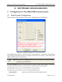
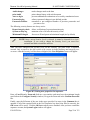
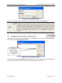
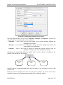
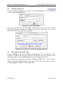
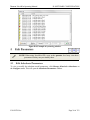
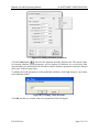
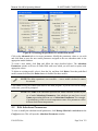
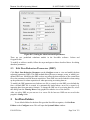
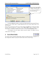
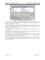
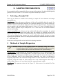
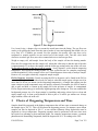

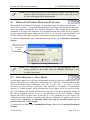
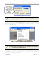
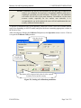
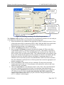
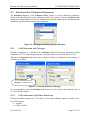
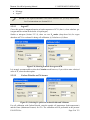
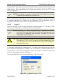
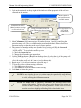
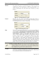
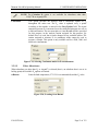
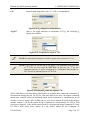
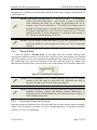
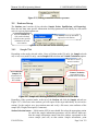
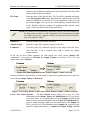
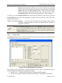
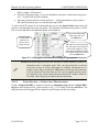
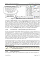
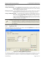
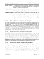
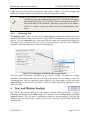
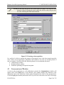
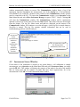

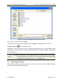
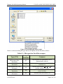
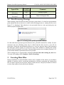
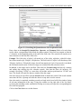
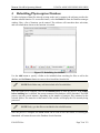
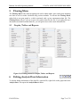
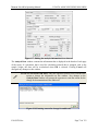
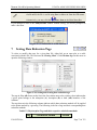
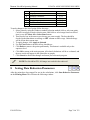
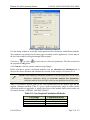
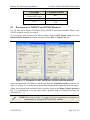
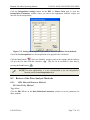
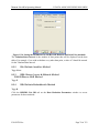
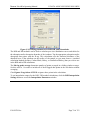
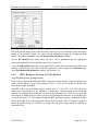
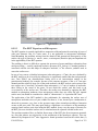
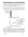
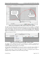
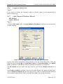
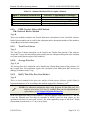
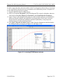
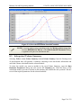
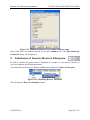
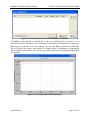
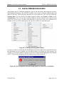
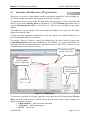
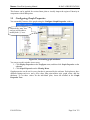
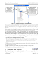
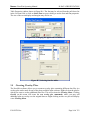
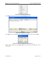
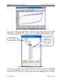
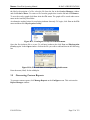
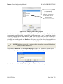
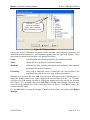
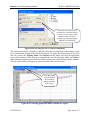
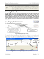

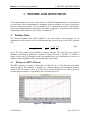
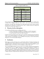
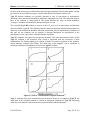
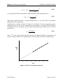
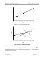
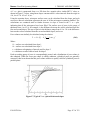
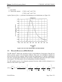
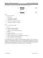
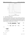
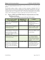
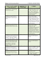
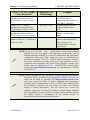
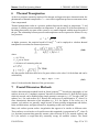


![[1 ] StorageTek SL8500](http://vs1.manualzilla.com/store/data/005684950_1-d7f31af8d49e38e9e4476c8a63e026d0-150x150.png)