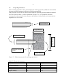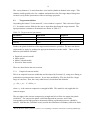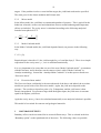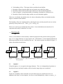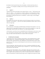
1
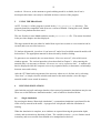
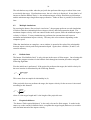
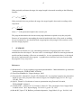
FFI RAPPORT MULTIFUNCTIONAL NUMERICAL TOOL FOR PENETRATION ANALYSIS TELAND Jan Arild FFI/RAPPORT-2002/04647 FFIBM/766/130 Approved Kjeller 27. November 2002 Bjarne Haugstad Director of Research MULTIFUNCTIONAL NUMERICAL TOOL FOR PENETRATION ANALYSIS TELAND Jan Arild FFI/RAPPORT-2002/04647 FORSVARETS FORSKNINGSINSTITUTT Norwegian Defence Research Establishment P O Box 25, NO-2027 Kjeller, Norway 3 UNCLASSIFIED FORSVARETS FORSKNINGSINSTITUTT (FFI) Norwegian Defence Research Establishment _______________________________ P O BOX 25 N0-2027 KJELLER, NORWAY SECURITY CLASSIFICATION OF THIS PAGE (when data entered) REPORT DOCUMENTATION PAGE 1) PUBL/REPORT NUMBER 2) FFI/RAPPORT-2002/04647 1a) PROJECT REFERENCE 3) NUMBER OF PAGES UNCLASSIFIED 2a) FFIBM/766/130 4) SECURITY CLASSIFICATION DECLASSIFICATION/DOWNGRADING SCHEDULE 18 - TITLE MULTIFUNCTIONAL NUMERICAL TOOL FOR PENETRATION ANALYSIS 5) NAMES OF AUTHOR(S) IN FULL (surname first) TELAND Jan Arild 6) DISTRIBUTION STATEMENT Approved for public release. Distribution unlimited. (Offentlig tilgjengelig) 7) INDEXING TERMS IN ENGLISH: IN NORWEGIAN: a) Cavity expansion a) Hulromsekspansjon b) Numerical tool b) Numerisk verktøy c) Matlab c) Matlab d) Penetration d) Penetrasjon e) e) THESAURUS REFERENCE: 8) ABSTRACT An advanced analytical/numerical tool for calculating penetration of rigid projectiles into various materials is described. The program is based on cavity expansion theory (CET) and is a further development of an earlier FFI-code to include numerous projectile geometries and target configurations. The new program also contains a graphical user interface making it very simple to define materials and set up penetration simulations. Moreover, it is possible to run multiple simulations to determine the penetration depth as a function of velocity, and the program can also determine ballistic limit and required target thickness to stop a projectile. This report serves as documentation and user manual for the program. 9) DATE AUTHORIZED BY POSITION This page only 27. November 2002 ISBN 82-464-0693-0 Bjarne Haugstad Director of Research UNCLASSIFIED SECURITY CLASSIFICATION OF THIS PAGE (when data entered) 5 CONTENTS Page 1 INTRODUCTION 7 2 GRAPHICAL USER INTERFACE 8 2.1 Projectile parameters 9 2.2 Target geometry parameters 10 2.3 2.3.1 2.3.2 2.3.3 2.3.4 Target material data Empirical concrete model Mises model Mohr-Coulomb model Piecewise linear model 11 11 12 12 12 3 BOUNDARY EFFECTS 12 3.1 Option 1 13 3.2 Option 2 13 3.3 Option 3 14 3.4 Option 4 14 3.5 Discussion 14 4 PENETRATION PHASES 14 5 USING THE PROGRAM 15 6 RUNNING SIMULATIONS 15 6.1 Single simulation 15 6.2 Multiple simulations 16 6.3 Ballistic limit 16 6.4 Required thickness 16 7 SUMMARY 17 Distribution list 18 7 MULTIFUNCTIONAL NUMERICAL TOOL FOR PENETRATION ANALYSIS 1 INTRODUCTION Penetration of a rigid projectile into a target material is often calculated using the theory of cavity expansion. In this approach, the stresses on a projectile during penetration is related to the radial stresses necessary for expanding a cavity at a given velocity. Analytical models of this kind do not yield a physical description comparable to full numerical simulations using Autodyn (or a similar code), but they are nonetheless very useful. It is much easier and quicker to obtain results from an analytical model than from a hydrocode, as the latter often requires a great deal of computation and modelling time. Analytical models are therefore useful for obtaining quick estimates or performing sensitivity studies varying various parameters. Furthermore, lack of accurate or reliable material data can render hydrocode simulations useless. There are three steps involved in using the cavity expansion theory (CET) to calculate penetration. First we calculate the radial stress pr on a cavity boundary as a result of a forced expansion at some velocity v. Secondly, we use this expression to estimate the stress pr (θ ) over a projectile surface during a penetration process, and integrate the stress to obtain the total force F on the projectile as a function of velocity. Finally, Newton’s 2nd law is applied to calculate the projectile motion. Of these steps, the first one is by far the most difficult as it involves solving a complicated set of differential equations. Depending on whether the target material model is simple enough, this can however be done analytically. For instance, this is the case for a Mises plasticity model. However, for a more complicated plasticity model, like a piecewise linear pressure dependent yield surface1, an analytical solution is not possible. In this case it becomes necessary to obtain a numerical solution for the cavity expansion force before proceeding to steps 2 and 3. In order to find a numerical solution easily, a numerical Matlab tool has been developed at FFI. It was first formulated in 1999 and documented in Norwegian (1), but has later been extended with several new options, including a graphical user interface. This report provides a brief documentation in English and also serves as a user manual for the new program. For details about the methods for numerical solution of the CET-equations, the reader is referred to (1). 1 This plasticity model has (incorrectly) been referred to as “Mohr-Coulomb” in Autodyn terminology. However, in Autodyn 5 it will be called “Drucker-Prager”, which is somewhat more accurate although still misleading. 8 For the Norwegian Defence Weapon Effects Handbook (2), a similar tool has been established independently. The difference between these tools is that the one described here is more aimed at the scientist/engineer who wants to experiment to see what happens when changes are made to material models (parameter/sensitivity studies), whereas the one in (2) is more aimed at the novice who needs a “quick result”. 2 GRAPHICAL USER INTERFACE The program can be run in two modes, either using the new graphical user interface (GUI) or the older textbased user interface. For a beginner, the GUI is clearly the easiest way to access the main program, while a more experienced user may prefer the other method. Figure 2.1: GUI of the Multifunctional Penetration Tool The GUI is shown in Figure 2.1. Most of the options should be self-explanatory, but for completeness we describe everything below. In order to completely define a penetration problem, it is necessary to define parameters related to both the projectile and the target. In the left column of the GUI, projectile parameters are defined, while target parameters are input in the right column. 9 2.1 Projectile parameters Some common projectiles can be selected from the “Select projectile” pull-down menu and the relevant projectile parameters will then be filled in automatically. If the projectile is not in the list, the user must input the required projectile parameters himself. These are listed in Table 2.1 and are illustrated in Figure 2.2. No explanation should be necessary about the projectile mass, diameter and impact velocity, but the two last parameters might deserve a few words. Flat part diameter Target thickness } Projectile curvature radius Cavity diameter Figure 2.2: Definition of projectile and target parameters. Table 2.1: Projectile parameters Parameter Projectile mass Projectile diameter Projectile curvature radius Flat part diameter Impact velocity Dimension kg cm cm cm m/s Required Yes Yes Yes No, default = 0 Yes Target diameter Projectile diameter 10 The parameter “projectile curvature” defines the curvature radius of the (ogival) projectile nose. The final parameter “flat part diameter” makes it possible to define a projectile with a truncated nose. The input value is then the diameter of the front part of the nose. If the nose is not truncated, this field can be left blank or set to zero. 2.2 Target geometry parameters The target geometry can be defined in the right part of the main menu of the GUI. The necessary input parameters are listed in Table 2.2. Table 2.2: Target geometry parameters Parameter Dimension Target diameter cm Target thickness cm Cavity diameter cm Figure 2.3: The graphical menu for defining material models. Required No, default = semi-infinite No, default = semi-infinite No, default = 0 11 The “cavity diameter” is used when there is an initial cylindrical channel in the target. This situation could typically arise for a tandem warhead where the first stage shaped charge has created a cavity before penetration of the second stage projectile. 2.3 Target material data On pushing the button ”Create material”, a new window is opened. This is shown in Figure 2.2. It contains various fields for the user to input data describing the target material. The input parameters common to all materials are shown in Table 2.3. Table 2.3: Target material parameters Parameter Dimension E-modulus GPa Poisson ratio ---Density kg/m3 Required Yes Yes Yes Further, the plastic behaviour of the target material must be specified. The user can choose which model to apply by pushing the appropriate button next to the model. There are four different yield models available: • • • • Empirical concrete model Mises model Mohr-Coulomb model Piecewise linear model These are described in the next sections. 2.3.1 Empirical concrete model This is an empirical concrete model that was developed by Forrestal (3), using curve fitting to penetration experiments into concrete. It was later modified by FFI (4) to hold for a larger range of concretes. Thus, the cavity radial stress is found from this formula: pr = Sσ c + ρ v 2 S = 49.5σ c−0.43 where σ c is the concrete compressive strength in MPa. This model is only applicable for concrete targets. The user input is the concrete compressive strength and (for a finite size target) the plastic yield limit2. For concrete the plastic yield limit depends on pressure, and a value corresponding to the high pressures encountered during a penetration process, should be entered. Note that the yield limit is only used in the calculation of boundary effects for finite 2 We use the term “plastic yield” for concrete, even if yielding is related to internal microcracking and damage. 12 targets. If the problem involves a semi-infinite target, the yield limit needs not be specified. The same goes for the elastic modulus and Poisson ratio. 2.3.2 Mises model In the Mises model, the yield limit is constant independent of pressure. This is typical for the behaviour of metals, such as steel and aluminium when no strain hardening and temperature effects are included. The cavity stress is calculated according to the following analytical formula from spherical CET: pr = 2.3.3 2Y E 1 + ln 3 3(1 − υ )Y Mohr-Coulomb model In the Mohr-Coulomb model, the yield limit depends linearly on pressure in the following way: Y = Y0 + β p Required input is therefore Y0 (the yield strength for p=0) and the slope β. There is no simple expression for the cavity stress pr , so it is calculated numerically. It is very important to be aware that our use of the term “Mohr-Coulomb model” is consistent with the literature, and is therefore not the same as what is called “Mohr-Coulomb” in Autodyn terminology. Instead the “Autodyn Mohr-Coulomb” is in this report referred to as “Piecewise linear”. 2.3.4 Piecewise linear model The Piecewise linear yield model is the most advanced of the three, and indeed, the two other models are special cases of the Piecewise model. Again, the yield stress depends on the pressure. The user has to input four pairs of (p,Y) datapoints, and the yield stress is then linearly interpolated. For pressures larger than the highest input, the yield stress is constant equal to the highest yield stress. Again the cavity stress pr has to be calculated numerically as no analytical solution is possible. This model is best suited for concrete and geological materials. 3 BOUNDARY EFFECTS Boundary effects can be accounted for in various different ways. This is selected in the box “Boundary option” on the right hand side of the menu. The following values are possible: 13 0. 1. 2. 3. 4. No boundary effects. The target is thus considered semi-infinite. Boundary effects from the edges but not from the rear end of the target. Boundary effects both from the edges and the rear end calculated separately. Same as Option 2 except that distance to boundary calculated in a different way. Boundary effects from the edges and the rear end calculated together. If the box is left blank, the default value is 0, thus no boundary effects are included and the target is considered semi-infinite. The boundary effects are implemented by reducing the stress on the projectile nose at various points by a decay factor α (θ ) . Thus, pr (θ ) → α (θ ) pr (θ ) There are several ways to define the decay factor. In our calculations an extension of an expression derived by Littlefield (5) is used: α= ln (1 + 4( xb / d ) ) 1 + ln( 3G / Y ) where xb is the distance to the boundary, which may depend on the position on the projectile nose. If α is larger than one, it is put equal to one. The distance xb is not uniquely defined, but different possibilities can be selected by the user. The various options are shown in Figure 3.1 and are described in detail below. Figure 3.1: Options 1-4 (left to right) for defining the distance to the boundary and the related decay factors. 3.1 Option 1 Using this option, xb is set equal to the target diameter. Thus α is independent of position on the projectile nose and only boundary effects from the target edges are considered. 3.2 Option 2 In this case, boundary effects from the rear end of the target are considered as well. In addition to the factor α1 from Option 1, the force is also multiplied by a factor α3 where xb is 14 the distance from the projectile tip to the rear boundary, so that the total decay factor is α = α1α 2 . As a consequence, boundary effects are larger when the projectile is close to perforating. 3.3 Option 3 Again the decay factor is the product of two separate factors α1 and α2. The first factor is the same as in Option 1. The second factor is found by defining xb as the perpendicular distance from a given point on the projectile nose to a line parallel to the rear end of the target. Since this depends on which point on the nose is considered, we then average over the complete nose to obtain α2. 3.4 Option 4 The boundary effects from the edge and the rear end of the targets are taken care of with one expression. The parameter xb is given by the smallest perpendicular distance either to the rear end or the target edge. 3.5 Discussion It is clear that there are advantages and disadvantages with all the various options. For a very sharp projectile, the perpendicular distance to the rear end will for example be very large, and thus boundary effects from the rear end will be very small using this method. At the moment we provide no clear recommendation about which option is most correct, so the user is encouraged to experiment with the various settings to obtain different estimates. In many cases there will be little difference in results for the various options. 4 PENETRATION PHASES A penetration process can be divided into various phases. In the calculations these are dealt with in different ways: During the tunneling phase, when the projectile nose is completely inside the target, expressions from cavity expansion are used to determine the stresses on the projectile nose. These stresses are then integrated over the whole nose to obtain the total force on the projectile. In the cratering phase, when the projectile nose is not yet completely embedded in the target, only the part of the nose that is inside the target is integrated over. The force thus grows larger as the projectile enters the target. If the target has a finite thickness, there is a third phase when part of the projectile nose has exited the target. Also in this case, only the nose that is still inside the target is integrated over. This exit phase model is probably not very realistic for brittle materials where scabbing will make sure that material is released from the target rear face long before the projectile actually 15 reaches it. However, at the moment no good scabbing model is available, but if one is developed, this feature can easily be included in future versions of the program. 5 USING THE PROGRAM At FFI, Version 1.0 of the program is stored in the p766/penetration directory. The program should be compatible with all newer versions of Matlab. During this work, Matlab 6.2 on a Unix platform has been used. The user first has to start Matlab and then run the penetrate.m file. The menus described in the previous chapters are then displayed. The target material data can either be loaded from a previous session or a new material can be created (and even saved for later use). To load an old material, just select “Load material” and a list of available material models will be described. The appropriate material is then selected by double-clicking. To generate a new material, the user must choose “Generate material”, after which a new window appears. The various inputs have been described in Chapter 2. After entering the material data, it is necessary to choose “Generate new cavity expansion data”. A waitbar will then be displayed while the computer uses cavity expansion theory to determine a relationship between stress and velocity. After the CET data has been generated, the user may either save it for later use by selecting “Save data”, or simply close the window and return to the main window, since the target material model is now stored in memory. 6 RUNNING SIMULATIONS After both the projectile and target data have been entered, penetration simulations may be run. There are several different “simulation modes”, each of which is described below. 6.1 Single simulation By pressing the button “Run single simulation”, a penetration simulation is performed for the exact velocity entered in the menu. A progress bar is displayed while the simulation is running. When the simulation is complete, new windows are opened showing the penetration depth, velocity and acceleration as functions of time. The variables/vectors x,v,a,t are further stored in memory and are accessible from Matlab to be manipulated as desired. 16 The calculations stop either when the projectile has perforated the target or when it has come to rest inside the target. If perforation occurs, the exit velocity is displayed. It may then be of interest to find the ballistic limit, i.e. the minimum impact velocity that achieves perforation, and the minimum target length that stops perforation. Either of these is possible, as described later. 6.2 Multiple simulations By pressing the button “Run multiple simulations”, the program performs several simulations in order to find the relationship between impact velocity and final penetration depth. The maximum impact velocity is the one entered in the menu system, while the minimum impact velocity is 100 m/s. Twenty simulations are performed at constant intervals between maximum and minimum impact velocity. This may take a few minutes depending on the computer speed. When the simulations are complete, a new window is opened with a plot of the relationship between impact velocity and final penetration depth. Again, these variables (Xi and Vi) are stored in memory. 6.3 Ballistic limit The button “Find ballistic limit” is only relevant in the cases of finite targets. On selecting this option, the program searches for the ballistic limit through an iteration procedure using the following algorithm. First the initial run is performed. If the projectile perforates the target, the initial velocity for the next iteration is determined by the following formula: ( i )2 v0(i +1) = v0(i )2 − vrest This comes from an empirical relationship in (6). If the projectile does not perforate the target, the impact velocity for the next run is increased according to this formula: L + l (i ) v0 x (i ) where L is the target length and l is the length of the projectile nose. v0(i +1) = 6.4 Required thickness The button “Find required thickness” is also only relevant for finite targets. It works in the same way as the search for ballistic limit, except that the target length (thickness) is varied in each iteration instead of the impact velocity. 17 If the projectile perforates the target, the target length is increased according to the following formula: 2 (i ) Vrest L = L (1 + ) V0 If the projectile does not perforate the target, the target length is decreased according to this expression: ( i +1) (i ) L(i ) + x ( i ) 2 (i ) where x is the penetration depth in the current cycle. L(i +1) = The program determines the least necessary target thickness required to stop the projectile. Because of uncertainties surrounding the material models and since effects such as scabbing are not accounted for, one should include an appropriate safety margin if the results are to be used for design purposes. 7 SUMMARY A numerical tool based on (1) for calculating penetration of rigid projectiles into various materials has been developed. The user can to a certain degree define his own target material models and how boundary effects are accounted for. As new penetration theory is developed, this can be implemented in the program. A graphical user interface has been created so that the program is very easy to use. References (1) Berthelsen P A, Cavity expansion og penetrasjonsmekanikk – Materialmodeller og numeriske løsningsmetoder, FFI/RAPPORT-99/04260 (2) Forsvarets Håndbok for Våpenvirkninger, 2002 (3) Forrestal M J, Altman B S, Cargile J D, Hanchack S J, An empirical equation for penetration depth of ogive nose projectiles into concrete targets, Int J Impact Engng Vol 15, No. 4, pp. 395-405, 1994 (4) Sjøl H, Teland J A, Prediction of concrete penetration using Forrestal’s formula, FFI/RAPPORT-99/04415 (5) Littlefield D L, Anderson Jr C E, Partom Y, Bless S J ”The penetration of steel targets finite in radial extent”, Int J. Impact Engng. Vol 19 No 1, pp 49 - 62, 1997 (6) Recht R F, Ipson T W, Ballistic perforation dynamics, J Appl Mech, 30, pp. 384-390, 1963 18 DISTRIBUTION LIST FFIBM Dato: 27 November 2002 RAPPORTTYPE (KRYSS AV) X RAPPORT NR. REFERANSE 2002/04647 RAPPORTENS DATO FFIBM/766/130 27 November 2002 RAPPORTENS BESKYTTELSESGRAD ANTALL EKS UTSTEDT ANTALL SIDER Unclassified 21 RAPPORTENS TITTEL FORFATTER(E) MULTIFUNCTIONAL NUMERICAL TOOL FOR PENETRATION ANALYSIS TELAND Jan Arild FORDELING GODKJENT AV FORSKNINGSSJEF: FORDELING GODKJENT AV AVDELINGSSJEF: RAPP NOTAT RR 18 EKSTERN FORDELING ANTALL 1 1 1 1 1 EKS NR TIL Forsvarsbygg v/ Leif Riis v/ Ragnar Bjørgaas v/ Helge Langberg v/ Tom Hermansen INTERN FORDELING ANTALL 9 1 1 1 1 1 2 EKS NR TIL FFI-Bibl FFI-ledelse FFIE FFISYS FFIBM FFIN Forfattereksemplar(er) Restopplag til Biblioteket Elektronisk fordeling: FFI-veven Bjarne Haugstad (BjH) Svein Rollvik (SRo) Eirik Svinsås (ESv) Henrik Sjøl (HSj) Knut B Holm (KBH) Svein E Martinussen (SEM) John F Moxnes (JFM) Jan Arild Teland (JTe) FFI-K1 Retningslinjer for fordeling og forsendelse er gitt i Oraklet, Bind I, Bestemmelser om publikasjoner for Forsvarets forskningsinstitutt, pkt 2 og 5. Benytt ny side om nødvendig.