Download User_Manual for Big Data Bench 2.1

Big Data Bench 2.1
User’s Manual
Contents
1 Background .................................................................................................................................... 3
2 Introduction of Big Data Bench 2.1 ............................................................................................... 3
2.1 Our Benchmarking Methodology ....................................................................................... 3
2.2 Chosen Data sets and Workloads ........................................................................................ 4
2.3 Use case .............................................................................................................................. 6
3 Prerequisite Software Packages ..................................................................................................... 7
4 Data Generation ............................................................................................................................. 8
4.1 Text Data ............................................................................................................................. 8
4.2 Graph Data .......................................................................................................................... 8
4.3 Table Data ........................................................................................................................... 9
5 Workloads .................................................................................................................................... 10
5.1 MicroBenchmarks ............................................................................................................. 10
5.1.1 Sort & Wordcount & Grep ..................................................................................... 10
5.1.2 BFS (Breath first search) ........................................................................................ 10
5.2 Basic Datastore Operations ............................................................................................... 11
5.2.1 Write ....................................................................................................................... 11
5.2.2 Read ....................................................................................................................... 12
5.2.3 Scan ........................................................................................................................ 14
5.3 Relational Query ............................................................................................................... 15
5.4 Search Engine ................................................................................................................... 16
5.4.1 Search Engine Web Serving ................................................................................... 16
5.4.2 SVM ....................................................................................................................... 16
5.4.3 PageRank ............................................................................................................... 16
5.4.4 Index....................................................................................................................... 16
5.5 Social Network.................................................................................................................. 17
5.5.1 Web Serving ........................................................................................................... 17
5.5.2 Kmeans................................................................................................................... 17
5.5.3 Connected Components ......................................................................................... 17
5.6 Ecommerce System ........................................................................................................... 18
5.6.1 Ecommerce System Web Serving .......................................................................... 18
5.6.2 Collaborative Filtering Recommendation .............................................................. 18
5.6.3 Bayes ...................................................................................................................... 19
6 Reference ..................................................................................................................................... 20
2
This document presents information on BigDataBench----a big data benchmark suite from web
search engines, including a brief introduction and the usage of it. The information and
specifications contained are for researchers who are interested in big data benchmarking.
Publishing information:
Release 2.1
Date 22/11/2013
Contact information:
Website: http://prof.ict.ac.cn/BigDataBench/
1 Background
BigDataBench is a big data benchmark suite from web search engines. Now, we provide the
second release of BigDataBench for downloading. In this edition, we pay attention to big data
workloads in three important applications domains in Internet services: search engine, social
networks, and electronic commerce according to a widely acceptable metrics—the number of page
views and daily visitors. The second release (BigDataBench 2.0) has 6 categories and 19 types’
big data applications which are the most important domain in Internet services. It also provides an
innovative data generation tool to generate scalable volumes of big data from a small-scale of real
data preserving semantics and locality of the real data. The data sets in BigDataBench are
generated by the tool. Users can also combine other applications in BigDataBench according to
their own requirements.
2 Introduction of Big Data Bench 2.1
2.1 Our Benchmarking Methodology
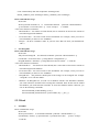
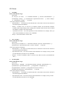
The philosophy of BigDataBench methodology is From Real System to Real System. We widely
investigate the typical Internet applications domains, then characterize the big data benchmark
from two aspects: data sets and workloads. The methodology of our benchmark is shown in
Figure1. First of all, we investigate the application category of Internet services, and choose the
dominant application domains for further characterizing based on the number of page views.
According to the analysis in [36], the top three application domains hold 80% page views of all
the Internet service. They are adopted in the BigDataBench application domain, which include
search engine, social networks and electronic commerce. These domains represent the typical
applications of Internet service, and the applications represent a wide range of categories to access
the big data benchmarking requirement of workload diversity.
3
Representative
Real Data Sets
Data types :
 Structured data
 Unstructured data
 Semi-Structured data
Data Sources：
 Table data
 Text data
 Graph data
 Extended
Big Data Sets
Preserving 4V
Synthetic data generation tool preserving data characteristics
Investigate
Typical
Application
Domains
Diverse and
Important
workloads
Basic & Important
Algorithms and
Operations
Extended ..
Application types :
 Offline analytics
 Realtime analytics
 Online services
BigDataBench:
Big Data
Benchmark Suite
Big Data
Workloads
Represent
Software Stack
Extended...
Figure1. BigDataBench Methodology
After choosing the application domains, we characterize the data sets and workloads of
BigDataBench based on the requirements proposed in the next subsection.
2.2 Chosen Data sets and Workloads
As analyzed in our article, the data sets should cover different data types of big data applications.
Based on the investigation of three application domains, we collect six representative real data sets.
Table 2 shows the characteristics of six real data sets and their corresponding workloads and Table
3 shows the Diversity of data sets. The original data is real, however, not big. We need to scale the
volume of the data while keep the veracity.
Table 2: The summary of six real data sets
Table3.Data Diversity
4
Further, we choose three different application domains to build our benchmark, because they
cover the most general big data workloads.
For search engine, the typical workloads are Web Serving, Index and PageRank. For web
applications, Web Serving is a necessary function module to provide an entrance for the service.
Index is also an important module, which is widely used to speed up the document searching
efficiency. PageRank is an important part to rank the searching results for search engines.
For ecommerce system, the typical workloads include Web Serving and Off-line Data Analysis.
The Web Serving workload shows information of products and provides a convenient platform for
users to buy or sell products. Off-line Data Analysis workload mainly does the data mining
calculation to promote the buy rate of products. In BigDataBench we select these Data Analysis
workloads: Collaborate Filtering and Bayes.
For social networking service, the typical workloads are Web Serving and graph operations. The
Web Serving workload aims to interactive with each user and show proper contents. Graph
operations are series of calculations upon graph data. In BigDataBench, we use Kmeans and
breath first search to construct the workloads of graph operation.
Besides, we defined three operation sets: Micro Benchmarks (sort, grep, word count and BFS),
Database Basic Datastore Operations(read/write/scan) and Relational Query(scan/aggregation/join)
to provide more workload choices.
Table 6: The Summary of BigDataBench.
(Benchmark i-(1,..,j) means 1th,..,j-th implementation of Benchmark i, respectively.)
By choosing different operations and environment, it's possible for users to compose specified
benchmarks to test for specified purposes. For example basic applications under MapReduce
environment can be chosen to test if a type of architecture is proper for doing MapReduce jobs.
5
2.3 Use case
This subsection will describe the application example of BigDataBench.
General procedures of using BigDataBench are as follows:
1. Choose the proper workloads. Select workloads with the specified purpose, for example basic
operations in Hadoop environment or typical search engine workloads.
2. Prepare the environment for the corresponding workloads. Before running the experiments, the
environment should be prepared first for example the Hadoop environment.
3. Prepare the needed data for workloads. Generally, it's necessary to generate data for the
experiments with the data generation tools.
4. Run the corresponding applications. With all preparations done, it's needed to start the workload
applications and/or performance monitoring tools in this step.
5. Collect results of the experiments.
Here we provide two usage case to show how to use our benchmark to achieve different
evaluating task.
Case one: from the perspective of maintainer of web site
If application scene and software are known, the maintainer want to choose suitable hardware
facilities. For example, someone have develop a web site of search engine, and use Hadoop, Hive,
Hbase as their infrastructures. Now he want evaluate if specifical hardware facilities are suitable
for his scene using our benchmark. First, he should select the workloads of search engine, saying
search web serving, indexing, and PageRank.
Also, the basic operations like sort, word count, and grep should be contained. To covering the
Hive and Hbase workload, he also should select the hive queries and read, write, scan of Hbase.
Next, he should prepare the environment and corresponding data. Finally, he runs each workloads
selected and observe the resluts to make evaluation.
Case two: from the perspective of architecture
Suppose that someone is planning to design a new machine for common big data usage. It is not
enough to run subset of the workloads, since he doesn't know what special application scene and
soft stack the new machine is used for. The comprehensive evaluation is needed, so that he should
run every workload to reflect the performance of different application scene, program framework,
data warehouse, and NoSQL database. Only in this way, he can say his new design is indeed
beneficial for big data usage.
6
Other use cases of BigDataBench include:
Web serving applications:
Using BigDataBench to study the architecture feature of Web Serving applications in big data
scenario(Search Engine).
Data Analysis workload’s feature:
Another kind of use case is to observe the typical data analysis workloads’(for example PageRank,
Recommendation) architectural characters.
Different storage system:
In BigDataBench, we also provide different data management systems(for example HBase,
Cassandra, hive). Users can choose one or some of them to observe the architectural feature by
running the basic operations(sort, grep, wordcount).
Different programing models:
Users can use BigDataBench to study three different programing models: MPI, MapReduce and
Spark.
3 Prerequisite Software Packages
Software
Version
Download
Hadoop
1.0.2
http://hadoop.apache.org/#Download+Hadoop
HBase
0.94.5
http://www.apache.org/dyn/closer.cgi/hbase/
Cassandra
1.2.3
http://cassandra.apache.org/download/
MongoDB
2.4.1
http://www.mongodb.org/downloads
Mahout
0.8
https://cwiki.apache.org/confluence/display/MAHOUT/Downloads
Hive
0.9.0
https://cwiki.apache.org/confluence/display/Hive/GettingStarted
#GettingStarted-InstallationandConfiguration
Spark
0.7.3
http://spark.incubator.apache.org/
Impala
1.1.1
http://www.cloudera.com/content/cloudera-content/
cloudera-docs/Impala/latest/Installing-and-Using-Impala/ciiu_install.html
MPICH
1.5
http://www.mpich.org/downloads/
GSL
1.16
http://www.gnu.org/software/gsl/
7
4 Data Generation
In Big Data Bench, We have three kinds of data generation tools to generate text data, graph data
and table data. Generally, the process contains two sub steps. The first step is to prepare for
generate big data by analyzing the characteristics of the seed data which is real owned by users,
and the second sub step is to expand the seed data to big data maintaining the features of seed
data.
4.1 Text Data
We provide a data generation tool which can generate data with user specified data scale. In
BigDataBench2.1 we analyze the wiki data sets to generate model, and our text data generate tool
can produce the big data based on the model.
Usage
Generate the data
Basic command-line usage:
sh gen_data.sh model_name number_of_files lines_per_file
<model_name>: the name of model used to generate new data
< number_of_files >: the number of files to generate
< lines_per_file >: number of lines in each file
For example:
sh gen_data.sh lda_wiki1w 10 10000
This command will generate 10 files each contains 10000 lines by using model wiki1w.
Note: The tool Need to install GSL - GNU Scientific Library. Before you run the program,
Please make sure that GSL is ready.
4.2 Graph Data
Here we use Kronecker to generate data that is both mathematically tractable and have all the
structural properties from the real data set. (http://snap.stanford.edu/snap/index.html)
In BigDataBench2.1 we analyze the Google, Facebook and Amazon data sets to generate model,
and our graph data generate tool can produce the big data based on the model.
8
Usage
Generate the data
Basic command-line usage:
./krongen \
-o:Output graph file name (default:'graph.txt')
-m:Matrix (in Maltab notation) (default:'0.9 0.5; 0.5 0.1')
-i:Iterations of Kronecker product (default:5)
-s:Random seed (0 - time seed) (default:0)
For example:
./krongen -o:../data-outfile/amazon_gen.txt -m:"0.7196 0.6313; 0.4833 0.3601" -i:23
4.3 Table Data
We use Parallel Data Generation Framework to generate table data. The Parallel Data Generation
Framework (PDGF) is a generic data generator for database benchmarking. PDGF was designed
to take advantage of today's multi-core processors and large clusters of computers to generate
large amounts of synthetic benchmark data very fast. PDGF uses a fully computational approach
and is a pure Java implementation which makes it very portable.
You can use your own configuration file to generate table data.
Usage
1. Prepare the configuration files
The configuration files are written in XML and are by default stored in the config folder.
PDGF-V2 is configured with 2 XML files: the schema configuration and the generation
configuration. The schema configuration (demo-schema.xml) defines the structure of the data and
the generation rules, while the generation configuration (demo-generation.xml) defines the output
and the post-processing of the generated data.
For the demo, we will generate the files demo-schema.xml and demo-generation.xml which are
also contained in the provided .gz file. Initially, we will generate two tables: OS_ORDER and
OS_ORDER_ITEM.
 demo-schema.xml
 demo-generation.xml
2. Generate data
After creating both demo-schema.xml and demo-generation.xml a first data generation run can be
performed. Therefore it is necessary to open a shell, change into the PDGFEnvironment directory.
Basic command-line usage:
java -XX:NewRatio=1 -jar pdgf.jar -l demo-schema.xml -l demo-generation.xml -c –s
9
5 Workloads
After generating the big data, we integrate a series of workloads to process the data in our big data
benchmarks. In this part, we will introduction how to run the Big Data Benchmark for each
workload. It mainly has two steps. The first step is to generate the big data and the second step is
to run the applications using the data we generated.
After unpacking the package, users will see six main folders General, Basic Operations, Database
Basic Operations, Data Warehouse Basic Operations, Search Engine, Social Network and
Ecommerce System.
5.1 MicroBenchmarks
5.1.1 Sort & Wordcount & Grep
Note: Please refer to BigDataBenchV1 for the above three workloads in MapReduce
environment. The MPI and Spark versions will be published soon.
5.1.2 BFS (Breath first search)
To prepare
1. Please decompress the file: BigDataBench_V2.1.tar.gz
tar xzf BigDataBench_V2.1.tar.gz
2. Open the DIR: graph500
cd BigDataBench_V2.1/MicroBenchmarks/BFS/graph500
Basic Command-line Usage:
mpirun -np PROCESS_NUM graph500/mpi/graph500_mpi_simple VERTEX_SIZE
Parameters:
PROCESS_NUM: number of process;
VERTEX_SIZE: number of vertex, the total number of vertex is 2^ VERTEX_SIZE
For example: Set the number of total running process of to be 4, the vertex number to be
2^20, the command is:
mpirun -np 4 graph500/mpi/graph500_mpi_simple 20
10
5.2 Basic Datastore Operations
We use YCSB to run database basic operations. And, we provide three ways: HBase, Cassandra
and MongoDB to run operations for each operation.
To Prepare
Obtain YCSB:
wget https://github.com/downloads/brianfrankcooper/YCSB/ycsb-0.1.4.tar.gz
tar zxvf ycsb-0.1.4.tar.gz
cd ycsb-0.1.4
Or clone the git repository and build:
git clone git://github.com/brianfrankcooper/YCSB.git
cd YCSB
mvn clean package
We name $YCSB as the path of YCSB for the following steps.
5.2.1 Write
1. For HBase
Basic command-line usage:
cd $YCSB
sh bin/ycsb load hbase -P workloads/workloadc -p threads=<thread-numbers> -p
columnfamily=<family> -p recordcount=<recordcount-value> -p hosts=<hostip> -s>load.dat
A few notes about this command:
 <thread-number> : the number of client threads, this is often done to increase the amount of
load offered against the database.
 <family> : In Hbase case, we used it to set database column. You should have database
usertable with column family before running this command. Then all data will be loaded
into database usertable with column family.
 <recorcount-value>: the total records for this benchmark. For example, when you want to
load 10GB data you shout set it to 10000000.
 <hostip> : the IP of the hbase’s master node.
2. For Cassandra
Before you run the benchmark, you should create the keyspace and column family in the
Cassandra. You can use the following commands to create it:
CREATE KEYSPACE usertable
with placement_strategy = 'org.apache.cassandra.locator.SimpleStrategy'
and strategy_options = {replication_factor:2};
use usertable;
11
create column family data with comparator=UTF8Type and
default_validation_class=UTF8Type and key_validation_class=UTF8Type;
Basic command-line usage:
cd $YCSB
sh bin/ycsb load cassandra-10 -P workloads/workloadc -p threads=<thread-numbers>
-p recordcount=<recorcount-value> -p hosts=<hostips> -s >load.dat
A few notes about this command:
 <thread-number> : the number of client threads, this is often done to increase the amount of
load offered against the database.
 <recorcount-value> : the total records for this benchmark. For example, when you want to
load 10GB data you shout set it to 10000000.
 <hostips> : the IP of cassandra’s nodes. If you have more than one node you should divide
with “,”.
3. For MongoDB
Basic command-line usage:
cd $YCSB
/bin/ycsb load mongodb -P workloads/workloadc -p threads=<thread-numbers> -p
recordcount=<recorcount-value> -p mongodb.url=<mongodb.url> -p
mongodb.database=<database> -p mongodb.writeConcern=normal -s >load.dat
A few notes about this command:
 <thread-number> : the number of client threads, this is often done to increase the amount of
load offered against the database.
 <recorcount-value>: the total records for this benchmark. For example, when you want to
load 10GB data you shout set it to 10000000.
 <mongodb.url>: this parameter should point to the mongos of the mongodb. For example
“mongodb://172.16.48.206:30000”.
 <database>: In Mongodb case, we used it to set database column. You should have database
ycsb with collection usertable before running this command. Then all data will be loaded
into database ycsb with collection usertable. To create the database and the collection, you
can use the following commands:
db.runCommand({enablesharding:"ycsb"});
db.runCommand({shardcollection:"ycsb.usertable",key:{ _id:1}});
5.2.2 Read
1. For HBase
Basic command-line usage:
cd $YCSB
sh bin/ycsb run hbase -P workloads/workloadc -p threads=<thread-numbers> -p
columnfamily=<family> -p operationcount=<operationcount-value> -p hosts=<hostip>
-s>tran.dat
12
A few notes about this command:
 <thread-number> : the number of client threads, this is often done to increase the amount of
load offered against the database.
 <family> : In Hbase case, we used it to set database column. You should have database
usertable with column family before running this command. Then all data will be loaded
into database usertable with column family.
 < operationcount-value >: the total operations for this benchmark. For example, when you
want to load 10GB data you shout set it to 10000000.
 <hostip> : the IP of the hbase’s master node.
2. For Cassandra
Basic command-line usage:
cd $YCSB
sh bin/ycsb run cassandra-10 -P workloads/workloadc -p threads=<thread-numbers> -p
operationcount=<operationcount-value> -p hosts=<hostips> -s>tran.dat
A few notes about this command:
 <thread-number> : the number of client threads, this is often done to increase the amount of
load offered against the database.
 <operationcount-value> : the total records for this benchmark. For example, when you want
to load 10GB data you shout set it to 10000000.
 <hostips> : the IP of cassandra’s nodes. If you have more than one node you should divide
with “,”.
3. For MongoDB
Basic command-line usage:
cd $YCSB
sh bin/ycsb run mongodb -P workloads/workloadc -p threads=<thread-numbers> -p
operationcount=<operationcount-value> -p mongodb.url=<mongodb.url> -p
mongodb.database=<database> -p mongodb.writeConcern=normal -p
mongodb.maxconnections=<maxconnections> -s>tran.dat
A few notes about this command:
 <thread-number> : the number of client threads, this is often done to increase the amount of
load offered against the database.
 <operationcount-value> : the total records for this benchmark. For example, when you want
to load 10GB data you shout set it to 10000000.
 <mongodb.url>: this parameter should point to the mongos of the mongodb. For example
“mongodb://172.16.48.206:30000”.
 <database>: In Mongodb case, we used it to set database column. You should have database
ycsb with collection usertable before running this command. Then all data will be loaded
into database ycsb with collection usertable. To create the database and the collection, you
can use the following commands:
db.runCommand({enablesharding:"ycsb"});
db.runCommand({shardcollection:"ycsb.usertable",key:{ _id:1}});
 <maxconnections> : the number of the max connections of mongodb.
13
5.2.3 Scan
1. For HBase
Basic command-line usage:
cd $YCSB
sh bin/ycsb run hbase
-P workloads/workloade -p threads=<thread-numbers> -p
columnfamily=<family> -p operationcount=<operationcount-value> -p hosts=<Hostip>
-p columnfamily=<family>
-s>tran.dat
A few notes about this command:
 <thread-number> : the number of client threads, this is often done to increase the amount of
load offered against the database.
 <family> : In Hbase case, we used it to set database column. You should have database
usertable with column family before running this command. Then all data will be loaded
into database usertable with column family.
 < operationcount-value >: the total operations for this benchmark. For example, when you
want to load 10GB data you shout set it to 10000000.
 <hostip> : the IP of the hbase’s master node.
2. For Cassandra
Basic command-line usage:
cd $YCSB
sh bin/ycsb run cassandra-10 -P workloads/workloade -p threads=<thread-numbers> -p
operationcount=<operationcount-value> -p hosts=<hostips> -s>tran.dat
A few notes about this command:
 <thread-number> : the number of client threads, this is often done to increase the amount of
load offered against the database.
 <operationcount-value> : the total records for this benchmark. For example, when you want
to load 10GB data you shout set it to 10000000.
 <hostips> : the IP of cassandra’s nodes. If you have more than one node you should divide
with “,”.
3. For MongoDB
Basic command-line usage:
cd $YCSB
sh bin/ycsb run mongodb -P workloads/workloade -p threads=<thread-numbers> -p
operationcount=<operationcount-value> -p mongodb.url=<mongodb.url> -p
mongodb.database=<database> -p mongodb.writeConcern=normal -p
mongodb.maxconnections=<maxconnections> -s>tran.dat
A few notes about this command:
 <thread-number> : the number of client threads, this is often done to increase the amount of
load offered against the database.
 <operationcount-value> : the total records for this benchmark. For example, when you want
to load 10GB data you shout set it to 10000000.
14
 <mongodb.url>: this parameter should point to the mongos of the mongodb. For example
“mongodb://172.16.48.206:30000”.
 <database>: In Mongodb case, we used it to set database column. You should have database
ycsb with collection usertable before running this command. Then all data will be loaded
into database ycsb with collection usertable. To create the database and the collection, you
can use the following commands:
db.runCommand({enablesharding:"ycsb"});
db.runCommand({shardcollection:"ycsb.usertable",key:{ _id:1}});
 <maxconnections> : the number of the max connections of mongodb.
5.3 Relational Query
To Prepare
Hive and Impala(including impala server and impala shell) should be installed. (Please refer to
<<Prerequisite>>)
1. Please decompress the file: BigDataBench_V2.1.tar.gz
tar xzf BigDataBench_V2.1.tar.gz
2. Open the DIR: RelationalQuery
cd BigDataBench_V2.1/RelationalQuery
3. We use the PDGF-V2 to generate data. Please refer to section 4.3<<Table Data>>
You can generate data by Table_datagen Tool.
cd BigDataBench_V2.1/DataGenerationTools/Table_datagen
java -XX:NewRatio=1 -jar pdgf.jar -l demo-schema.xml -l demo-generation.xml -c -s
mv output/ ../../RelationalQuery/data-RelationalQuery
4. Before importing data, please make sure the ‘hive’ and ‘impala-shell’ command are available
in your shell environment. You can import data to Hive in this manner:
Load data to hive.
sh prepare_RelationalQuery.sh [ORDER_TABLE_DATA_PATH]
[ITEM_TABLE_DATA_PATH]
Parameters:
ORDER_TABLE_DATA_PATH: path of the order table;
ITEM_TABLE_DATA_PATH: path of the item table.
Output: some log info.
To Run
Basic command-line usage:
sh run_RelationalQuery.sh [hive/impala] [select/aggregation/join]
Output: query result
15
5.4 Search Engine
Search engine is a typical application in big data scenario. Google, Yahoo, and Baidu accept huge
amount of requests and offer the related search results every day. A typical search engine crawls
data from the web and indexes the crawled data to provide the searching service.
5.4.1 Search Engine Web Serving
5.4.2 SVM
Note: Please refer to BigDataBench v1 for more information about these two
workloads.
5.4.3 PageRank
The PageRank program now we use is obtained from Hibench.
To prepare and generate data:
tar xzf BigDataBench_V2.1.tar.gz
cd BigDataBench_V2.1/SearchEngine/PageRank
sh genData_PageRank.sh
To run:
sh run_PageRank.sh [#_of_nodes] [#_of_reducers] [HDFS edge_file_path] [makesym or
nosym]
5.4.4 Index
The Index program now we use is obtained from Hibench.
To prepare:
tar xzf BigDataBench_V2.1.tar.gz
cd BigDataBench_V2.1/SearchEngine/Index
sh prepare.sh
Basic command-line usage:
sh run_Index.sh
16
5.5 Social Network
Social networking service has becoming a new typical big data application. A typical social
networking service generally contains a convenient a web serving module for users to view and
publish information. Besides, it has an efficient graph computation module to generate graph data
(for friend recommendation etc.) for each user.
5.5.1 Web Serving
We use the Web Serving workload of CloudSuite to construct the Web Serving of Social Network
System.
Please refer to http://parsa.epfl.ch/cloudsuite/web.html for setup.
5.5.2 Kmeans
The Kmeans program we used is obtained from Mahout.
To Prepare
tar xzf BigDataBench_V2.1.tar.gz
cd BigDataBench_V2.1/SNS/Kmeans
sh genData_Kmeans.sh
Basic command-line usage:
sh run_Kmeans.sh
5.5.3 Connected Components
The Connected Components program we used is obtained from PEGASUS.
To Prepare
tar xzf BigDataBench_V2.1.tar.gz
cd BigDataBench_V2.1/SNS/Connected_Components
sh genData_connectedComponents.sh
Basic command-line usage:
sh run_connectedComponents.sh [#_of_nodes] [#_of_reducers] [HDFS edge_file_path]
[#_of_nodes] : number of nodes in the graph
[#_of_reducers] : number of reducers to use in hadoop. - The number of reducers to use depends
on the setting of the hadoop cluster. - The rule of thumb is to use (number_of_machine * 2) as the
number of reducers.
[HDFS edge_file_path] : HDFS directory where edge file is located
17
5.6 Ecommerce System
A typical ecommerce system provides a friendly web serving, reliable database system and rapid
data analysis module. The database system stores information of items, users and biddings. Data
analysis is an important module of ecommerce system to analyze users’ feature and then promote
the bidding amounts by giving the proper recommendation.
With the development of related technologies, E-commerce has already become one of the most
important applications on internet. Our big data benchmarking work used various state-of-art
algorithms or techniques to access, analyze, store big data and offer E-commerce as follows.
5.6.1 Ecommerce System Web Serving
We use open source tool RUBiS as our Web service and data management workloads Application.
Since ten years ago, when E-commerce just became unfolding, it has attracted lot of researchers
researching its workload characteristics. RUBiS is an auction site prototype modeled after Ebay
that is used to evaluate application design patterns and application servers’ performance scalability.
The site implements the core functionality of an auction site: selling, browsing and bidding. To run
a RUBiS system, please reference to the RUBiS website: http://rubis.ow2.org/index.html.
The download URL is http://forge.ow2.org/project/showfiles.php?group_id=44
You can change the parameters of the payload generator (RUBiS/Client/rubis.properties) for what
you need.
Basic command-line usage:
vim $RUBiS_HOME/Client/rubis.properties
make emulator
5.6.2 Collaborative Filtering Recommendation
Collaborative filtering recommendation is one of the most widely used algorithms in E-com
analysis. It aims to solve the prediction problem where the task is to estimate the preference of a
user towards an item which he/she has not yet seen.
We use the RecommenderJob in Mahout(http://mahout.apache.org/) as our Recommendation
workload, which is a completely distributed itembased recommender. It expects ID1, ID2, value
(optional) as inputs, and outputs ID1s with associated recommended ID2s and their scores. As you
know, the data set is a kind of graph data.
Before you run the RecommenderJob, you must have HADOOP and MAHOUT prepared. You can
use Kronecker (see 4.2.1) to generate graph data for RecommenderJob.
18
Basic command-line usage:
tar xzf BigDataBench_V2.1.tar.gz
cd BigDataBench_V2.1/E-commerce
sh genData_recommendator.sh
sh run_recommendator.sh
Input parameters according to the instructions:
1. The DIR of your working derictor;
2. The DIR of MAHOUT_HOME.
5.6.3 Bayes
Naive Bayes is an algorithm that can be used to classify objects into usually binary categories. It is
one of the most common learning algorithms in Classification. Despite its simplicity and rather
naive assumptions it has proven to work surprisingly well in practice.
We use the naivebayes in Mahout(http://mahout.apache.org/) as our Bayes workload, which is a
completely distributed classifier.
Basic command-line usage:
tar xzf BigDataBench_V2.1.tar.gz
cd BigDataBench_V2.1/E-commerce
sh genData_naivebayes.sh
sh run_naivebayes.sh
Input parameters according to the instructions:
1. The DIR of your working derictor;
2. The DIR of MAHOUT_HOME.
19
6 Reference
[1] http://www-01.ibm.com/software/data/bigdata/.
[2] http://hadoop.apache.org/mapreduce/docs/current/gridmix.html.
[3] https://cwiki.apache.org/confluence/display/PIG/PigMix.
[4] “Amazon movie reviews,” http://snap.stanford.edu/data/web-Amazon.html.
[5] “Big data benchmark by amplab of uc berkeley,” https://amplab.cs.berkeley.edu/benchmark/.
[6] “facebook graph,” http://snap.stanford.edu/data/egonets-Facebook.html.
[7] “google web graph,” http://snap.stanford.edu/data/web-Google.html.
[8] “graph 500 home page,” http://www.graph500.org/.
[9] “Snap home page,” http://snap.stanford.edu/snap/download.html.
[10] “Sort benchmark home page,” http://sortbenchmark.org/.
[11] “Standard performance evaluation corporation (spec),”http://www.spec.org/.
[12] “Transaction processing performance council (tpc),”http://www.tpc.org/.
[13] “wikipedia,” http://en.wikipedia.org.
[14] Ghazal. A, “Big data benchmarking-data model proposa,” in FirstWorkshop on Big Data
Benchmarking, San Jose, Califorina, 2012.
[15] Timothy G Armstrong, Vamsi Ponnekanti, Dhruba Borthakur, andMark Callaghan,
“Linkbench: a database benchmark based on thefacebook social graph,” 2013.
[16] L.A. Barroso and U. Hölzle, “The datacenter as a computer: An introductionto the design of
warehouse-scale machines,” Synthesis Lectures on Computer Architecture, vol. 4, no. 1, pp.
1–108, 2009.
[17] M. Beyer, “Gartner says solving big data challenge involves more than just managing
volumes of data.”http://www.gartner.com/it/page.jsp?id=1731916.
[18] David M Blei, Andrew Y Ng, and Michael I Jordan, “Latent dirichlet allocation,” the Journal
of machine Learning research, vol. 3, pp. 993–1022, 2003.
[19] Deepayan Chakrabarti and Christos Faloutsos, “Graph mining: Laws, generators, and
algorithms,” ACM Computing Surveys (CSUR), vol. 38, no. 1, p. 2, 2006.
[20] Deepayan Chakrabarti, Yiping Zhan, and Christos Faloutsos, “R-mat: A recursive model for
graph mining,” Computer Science Department, p. 541, 2004.
[21] Brian F. Cooper, Adam Silberstein, Erwin Tam, Raghu Ramakrishnan, and Russell Sears,
“Benchmarking cloud serving systems with ycsb,” in Proceedings of the 1st ACM symposium on
Cloud computing, ser. SoCC ’10. New York, NY, USA: ACM, 2010, pp. 143–154. [Online].
Available: http://doi.acm.org/10.1145/1807128.1807152
[22] Cliff Engle, Antonio Lupher, Reynold Xin, Matei Zaharia, Michael J Franklin, Scott Shenker,
and Ion Stoica, “Shark: fast data analysis using coarse-grained distributed memory,” in
Proceedings of the 2012 ACM SIGMOD International Conference on Management of Data. ACM,
2012, pp. 689–692.
[23] Vuk Ercegovac, David J DeWitt, and Raghu Ramakrishnan, “The texture benchmark:
measuring performance of text queries on a relational dbms,” in Proceedings of the 31st
international conference on Very large data bases. VLDB Endowment, 2005, pp. 313–324.
[24] M. Ferdman, A. Adileh, O. Kocberber, S. Volos, M. Alisafaee, D. Jevdjic, C. Kaynak, A.
Popescu, A. Ailamaki, and B. Falsafi, “Clearing the clouds: A study of emerging workloads on
20
modern hardware,” Architectural Support for Programming Languages and Operating Systems,
2012.
[25] Ahmad Ghazal, Minqing Hu, Tilmann Rabl, Francois Raab, Meikel Poess, Alain Crolotte, and
Hans-Arno Jacobsen, “Bigbench: Towards an industry standard benchmark for big data analytics,”
in sigmod 2013. ACM, 2013.
[26] Ahmad Ghazal, Tilmann Rabl, Minqing Hu, Francois Raab, Meikel Poess, Alain Crolotte, and
Hans-Arno Jacobsen, “Bigbench: Towards an industry standard benchmark for big data analytics,”
2013.
[27] S. Huang, J. Huang, J. Dai, T. Xie, and B. Huang, “The hibench benchmark suite:
Characterization of the mapreduce-based data analysis,” in Data Engineering Workshops
(ICDEW), 2010 IEEE 26th International Conference on. IEEE, 2010, pp. 41–51.
[28] Jure Leskovec, Deepayan Chakrabarti, Jon Kleinberg, Christos Faloutsos, and Zoubin
Ghahramani, “Kronecker graphs: An approach to modeling networks,” The Journal of Machine
Learning Research, vol. 11, pp. 985–1042, 2010.
[29] Jurij Leskovec, Deepayan Chakrabarti, Jon Kleinberg, and Christos Faloutsos, “Realistic,
mathematically tractable graph generation and evolution, using kronecker multiplication,” in
Knowledge Discovery in Databases: PKDD 2005. Springer, 2005, pp. 133–145.
[30] Pejman Lotfi-Kamran, Boris Grot, Michael Ferdman, Stavros Volos, Onur Kocberber, Javier
Picorel, Almutaz Adileh, Djordje Jevdjic, Sachin Idgunji, Emre Ozer et al., “Scale-out
processors,” in Proceedings of the 39th International Symposium on Computer Architecture.
IEEE Press, 2012, pp. 500–511.
[31] Andrew Pavlo, Erik Paulson, Alexander Rasin, Daniel J. Abadi, David J. DeWitt, Samuel
Madden, and Michael Stonebraker, “A comparison of approaches to large-scale data analysis,” in
Proceedings of the 2009 ACM SIGMOD International Conference on Management of data, ser.
SIGMOD ’09. New York, NY, USA: ACM, 2009, pp. 165–178. [Online]. Available:
http://doi.acm.org/10.1145/1559845.1559865
[32] Tilmann Rabl, Michael Frank, Hatem Mousselly Sergieh, and Harald Kosch, “A data
generator for cloud-scale benchmarking,” in Performance Evaluation, Measurement and
Characterization of Complex Systems. Springer, 2011, pp. 41–56.
[33] Margo Seltzer, David Krinsky, Keith Smith, and Xiaolan Zhang, “The case for
application-specific benchmarking,” in Hot Topics in Operating Systems, 1999. Proceedings of the
Seventh Workshop on. IEEE, 1999, pp. 102–107.
[34] YC Tay, “Data generation for application-specific benchmarking,” VLDB, Challenges and
Visions, 2011.
[35] Matei Zaharia, Mosharaf Chowdhury, Tathagata Das, Ankur Dave, Justin Ma, Murphy
McCauley, Michael Franklin, Scott Shenker, and Ion Stoica, “Resilient distributed datasets: A
fault-tolerant abstraction for in-memory cluster computing,” in Proceedings of the 9th USENIX
conference on Networked Systems Design and Implementation. USENIX Association, 2012, pp.
2–2.
[36] J. Zhan, L. Zhang, N. Sun, L.Wang, Z. Jia, and C. Luo, “High volume throughput computing:
Identifying and characterizing throughput oriented workloads in data centers,” in Parallel and
Distributed Processing Symposium Workshops & PhD Forum (IPDPSW), 2012 IEEE 26th
International. IEEE, 2012, pp. 1712–1721.
[37] Zhen Jia, Lei Wang, Jianfeng Zhan, Lixin Zhang, and Chunjie Luo, Characterizing data
21
analysis workloads in data centers, 2013 IEEE International Symposium on Workload
Characterization (IISWC 2013).
22