Download Drawing power law graph - University of South Carolina

Drawing Power Law Graphs using a Local/Global Decomposition
∗
Reid Andersen
Fan Chung
University of California, San Diego
University of California, San Diego
Linyuan Lu
University of South Carolina
Abstract
It has been noted that many realistic graphs have a power law degree distribution and exhibit the small
world phenomenon. We present drawing methods influenced by recent developments in the modeling of
such graphs. Our main approach is to partition the edge set of a graph into “local” edges and “global”
edges, and to use a force-directed method that emphasizes the local edges. We show that our drawing
method works well for graphs that contain underlying geometric graphs augmented with random edges,
and demonstrate the method on a few examples. We define edges to be local or global depending on
the size of the maximum short flow between the edge’s endpoints. Here, a short flow, or alternatively
an `-short flow, is one composed of paths whose length is at most some constant `. We present fast
approximation algorithms for the maximum short flow problem, and for testing whether a short flow of a
certain size exists between given vertices. Using these algorithms, we give a fast approximation algorithm
for determining local subgraphs of a given graph. The drawing algorithm we present can be applied to
general graphs, but is particularly well-suited for numerous small-world networks with power law degree
distribution.
1
Introduction
Although graph theory has a history of more than 250 years, it was only recently observed that many realistic
graphs from disparate areas satisfy the so-called “power law”, where the fraction of nodes with degree k is
proportional to k −β for some positive exponent β. Graphs with power law degree distribution are prevalent
in the Internet, in communication networks, social networks and in biological networks [1, 2, 4, 5, 6, 9, 10,
13, 15, 20, 23, 24, 27]. Many real examples of networks also exhibit a so-called “small world phenomenon”
consisting of two distinct properties — small average distance between nodes, and a clustering effect where
two nodes sharing a common neighbor are more likely to be adjacent. It was shown in [11] that a random
power law graph has small average distance and small diameter. However, random power law graphs do not
adequately capture the clustering effect.
In [3], the authors introduced a hybrid graph model where a random power law graph called the global
graph is added to an underlying local graph. A local graph is a graph where the endpoints of each edge are
highly locally connected by large short flows. In particular, a graph is said to be (f, `)-local if the endpoints
of each edge are connected by an `-short flow of size f . Random geometric graphs and d-dimensional grid
graphs are good examples of local graphs for various parameters. Given an arbitrary graph G, we can choose
parameters f and ` and define the local graph of G to be its largest (f, `)-local subgraph, providing a way
to partition G into local and global edges. The main result of [3] is that the local graph of a hybrid graph is
∗ Research
1A
supported in part by NSF Grants DMS 0100472 and ITR 0205061
conference version appeared in Proceedings of the Twelfth Annual Symposium on Graph Drawing, 2004
1
equal to the original local graph up to a small error, indicating that local graphs are robust to the addition
of random edges.
In this paper we demonstrate that partitioning a graph into local and global edges based on local connectivity can be done quickly, and can be useful in graph drawing. To obtain local/global partitions for large
graphs, we present an approximation algorithm for computing the local graph. We also give a new algorithm
for the fundamental problem of computing the maximum short flow between given vertices. The number
of iterations required in our maximum short flow algorithm depends on the value fopt of the maximum
short flow. We also give a new algorithm for the problem of local connectivity testing, where we wish to
determine whether there exists a short flow of a certain size ftest between given vertices. The number of
iterations required by our testing algorithm is determined by ftest and not fopt , so testing local connectivity
can be done significantly faster than computing the maximum short flow. Our algorithms are based on the
maximum multicommodity flow algorithm of Garg and Könemann [17].
After obtaining a local/global partition, we use it by modifying a standard force-directed algorithm
to emphasize local edges. We demonstrate that this method produces improved drawings for graphs that
contain underlying geometric graphs augmented with random edges. This is theoretically supported, since
the robustness of the local graph implies that most of the edges in the underlying geometric graph will be
classified as local, while most of the edges from the random graph will be classified as global.
We also present a drawing method based on a more sophisticated partition that reflects other aspects
of the structure of power law graphs. For example, it was shown in [11] that a random power law graph
has roughly an “octopus” shape, with a dense “core” and a myriad of “tentacles” attached. While the core
itself may be a dense graph that is not amenable to most drawing methods, our algorithm takes advantage
of the local subgraph and the sparse tree-like structures in the tentacles, yielding improved drawings. This
partition extends the class of graphs for which the local/global partition is useful to many realistic networks
where some notion of closeness between vertices is reflected in the edge set.
2
Preliminaries
In [3], the authors introduced local graphs, which are graphs where the endpoints of each edge are highly
locally connected by a large short flow. In this section we introduce short flows and define local graphs. We
will also state a theorem showing that local graphs are robust to the addition of random edges. Throughout
the paper, the graphs we consider are undirected and unweighted.
2.1
Short Flows and Local Connectivity
There are a number of ways to define local connectivity between two given vertices u and v. A natural
approach is to consider the connectivity through paths whose length is at most some fixed constant `, which
we will call `-short paths or simply short paths. The path connectivity a` (u, v) is the maximum size of
an `-short collection of edge-disjoint u − v paths. The cut connectivity c` (u, v) is the minimum size of an
`-short u − v cut, a set of edges whose removal leaves no `-short u − v paths. The analogous version of
Menger’s theorem does not hold when we restrict to short paths— a` (u, v) and c` (u, v) are not necessarily
equal. However, it is easy to see that the trivial relations a` ≤ c` ≤ ` · a` still hold.
Both a` (u, v) and c` (u, v) are difficult to compute. In particular, computing the maximum number of
short disjoint paths is N P-hard if ` ≥ 4 [19]. In light of this result we will define local connectivity based on
maximum short flow, which we will define shortly, and which can be efficiently computed, as we will show
in Section 3.
2
An `-short flow is a linear combination of `-short paths where each edge has congestion at most 1. If
we let A be the incidence matrix where each column represents a `-short path from u to v and each row
represents an edge in the graph, then finding f` (u, v), the maximum `-short flow between u and v, can be
viewed as the following linear program.
f` (u, v) = max{ ~1T x | Ax ≤ ~1, x ~0 }.
(1)
The linear programming dual of the maximum short flow
P problem is a fractional cut problem. An `-short
fractional cut is a weight function w : E → R+ such that e∈P c(e) ≥ 1 for every `-short u −P
v path P . The
dual of the `-short maximum flow problem is to find an `-short fractional cut that minimizes e∈G c(e). We
let w` (u, v) denote the size of a minimum `-short fractional cut, and note that LP duality implies
a` (u, v) ≤ f` (u, v) = w` (u, v) ≤ c` (u, v).
(2)
Definition 1 Two vertices u and v are (f, `)-connected if f` (u, v) ≥ f .
Since all the coefficients in the incidence matrix, cost vector, and constraint vector in the problem
formulation (1) are nonnegative, the maximum short flow problem belongs to a special subset of linear
programs called fractional packing problems, for which there exist general techniques that often lead to
polynomial time algorithms [29]. In Section 3 we present a fast primal-dual algorithm for computing the
maximum `-short flow. We will also present an algorithm to test whether two vertices are (f, `)-connected,
which can be significantly faster than computing the maximum `-short flow.
2.2
Mengerian Theorems for Short Paths
It was mentioned previously that a` (u, v) and c` (u, v) are not necessarily equal. It is an open problem to
determine how much these quantities can differ with respect to `. It was shown by Lovász, Neumann-Lara,
and Plummer [26] that c` ≤ 2` · a` . Boyles and Exoo [8] have given a family of graphs where c` ≥ 4` · a` . Their
results were stated for the case of vertex-disjoint paths, but the results convert easily to the edge-disjoint
case which we are considering. We now present a simple construction showing that c` ≥ 3` · a` for infinitely
many `, improving the best known lower bound. We conjecture that c` ≤ 3` + o(1) · a` for all graphs.
Theorem 1 For every ` there exists a graph such that a` (u, v) = 1 and c` (u, v) ≥ 3` .
Proof: Consider a path P = x1 . . . x2n of length 2n − 1. We add 2n disjoint paths of length 2 between each
pair of adjacent vertices xi and xi+1 . Call this graph G2n , and let u = x1 and v = xn .
We refer to the edges of P as base edges. It is easy to see that an s − t path using at most k base edges
has length at least (4n − 2) − k. If we set ` = 3n − 2, then every `-short path must use at least n base edges
so that its length is at most (4n − 2) − n = 3n − 2 = `. Since there are only 2n − 1 base edges, any two
`-short paths must intersect in a base edge, so a` (u, v) = 1. We now consider the size of a minimum `-short
cut C. Without loss of generality we can assume that C cuts only base edges. If C cuts n − 1 or fewer base
edges, then n base edges remain and the path that proceeds from xi to xi+1 by taking a base edge whenever
possible has length at most (4n − 2) − (n) = 3n − 2 = `. Thus, c` (u, v) ≥ n, and so
c` (u, v) =
n
`
·`≥ .
3n − 2
3
It is not hard to modify the above construction to obtain examples for ` = 3n − 1 and ` = 3n with
c` (u, v) ≥ 3` . We can increase ` by 1 or 2 without changing a` (u, v) or c` (u, v) if we add a vertex x0 , let
u = x0 , and connect x0 to x1 with 2n paths of length 1, or 2n paths of length 2.
3
2.3
Local Graphs
Definition 2 A graph L is (f, `)-local if for each edge (u, v) in L, the endpoints u and v are (f, `)-connected
in L.
For example, the toroidal grid graph Cn × Cn is (3, 3)-local. This graph is also (4, 5)-local, which is slightly
less obvious and highlights the difference between a` (u, v) and f` (u, v). A 4-short flow of size 5 between the
endpoints of a grid edge is shown in the figure below. The correct combination to take is 1 of the path in
the grid on the left, and (1/2) of each path in the remaining grids.
v
v
u
u
v
u
v
u
Figure 1: A 5-bounded flow of size 4 between endpoints of a grid edge.
The union of two (f, `)-local graphs is (f, `)-local, and so there is a unique largest (f, `)-local subgraph of
G, which we denote Lf,` (G). In Section 4 we will present approximation algorithms for computing Lf,` (G).
It is important to note that Lf,` (G) is not necessarily connected.
2.4
Random Graphs with Specified Expected Degree Sequence
A random graph G(w) with specified expected degree sequence w = (w1 , wP
2 , . . . , wn ), is formed by including
each edge vi vj independently with probability pij = wi wj ρ, where
ρ
=
(
wi )−1 . It is easy to check that
P
2
vertex vi has expected degree wi . We assume that maxi wi < k wk so that pij ≤ 1 for all i and j. This
condition also implies that the sequence wi is graphical [14] if the wi are integers. This model has a non-zero
probability of self-loops, but the expected number of loops is of lower order than the total number of edges.
The typical random graph G(n, p) on n vertices with edge probability p is a random graph with expected
degree sequence w = (pn, pn, . . . , pn). For a subset S of vertices, we define
X
X
Vol(S) =
wi
and
Volk (S) =
wik .
vi ∈S
vi ∈S
Let d denote the average degree V ol(G)/n, and let d˜ denote the second-order average degree Vol2 (G)/Vol(G).
We also let m denote the maximum weight among the wi .
2.5
Robustness of Local Graphs
We consider how the local graph Lf,` (G) changes with the addition of random edges. In particular we
consider the addition of the edge set of a random graph G(w) with a specified expected degree sequence.
The following theorem states that local graphs are robust to the addition of these edge sets, provided the
random graph is not too dense. Graphs formed by the union of a local graph L and a random graph G(w)
were considered in [3], and were there called hybrid graphs.
4
Theorem 2 Let L be an (f, `)-local graph with maximum degree M . Let G(w) be a random graph from the
˜ and maximum weight
specified expected degree model with average
weight d, second order average weight d,
S
m. Let H be the hybrid graph H = G L, and let Lf,` (H) be the unique largest (f, `)-local subgraph of H.
If d˜ satisfies
d˜ ≤ nα ≤
nd
m2
1/`
n−3/f ` for some constant α > 0,
Then with probability 1 − O(n−1 ):
˜ edges.
1. L0 \ L contains O(d)
2. dL0 (x, y) ≥ 1` dL (x, y) for every pair x, y ∈ L.
The proof of this theorem is contained in [3].
3
Fast Algorithms for Short Flow Problems
Garg and Könemann [17] gave simple combinatorial algorithms for maximum multicommodity flow, maximum concurrent flow, and general fractional packing problems. We present a simple primal-dual approximation algorithm for the maximum short flow problem based on their techniques. The number of iterations
required by our algorithm is smaller than the number required by the algorithms for maximum multicommodity flow or general fractional packing problems. This is because the number of iterations in our algorithm can
be bounded in terms of f` (u, v), whereas the stated bounds for the multicommodity flow algorithm depends
on M .
Since we are computing `-short flows, our algorithms only need to consider the edges involved in some
`-short u, v path, which are all contained in the subgraph N`/2 (u) ∪ N`/2 (v). Thus, our running times will
be bounded in terms of m, the number of edges in the small subgraph N`/2 (u) ∪ N`/2 (v), and not on M , the
number of edges in the entire graph.
In our applications, we will be repeatedly testing whether two given vertices are (f, `)-connected for some
constants f and `, which we call the local connectivity testing problem. We combine our maximum short
flow algorithm with a greedy path selection algorithm to obtain an algorithm for local connectivity testing
where the number of iterations required depends on the constant f rather than f` (u, v). Thus, in many cases
we can test local connectivity much faster than we can compute the maximum short flow.
3.1
Computing the Maximum Short Flow
Maximum Short Flow:
The algorithm produces an `-short flow f by routing one unit of flow at each time step.
Initially,
Let w0 be a weight function w0 : E → R+ assigning weight δ to every edge in N`/2 (u) ∪ N`/2 (v).
Let f0 be the empty flow.
At each time step i,
Let p(i) be an `-short path of minimum weight with respect to the current weight function wi .
Let α(i) be the weight of this path.
Modify f by routing 1 unit of flow on p(i),
5
Modify the weight function by setting wi+1 (e) = wi (e) · (1 + ) for each edge e ∈ p(i).
The procedure stops at the first time step t when α(t) ≥ 1.
The flow f (t) is then scaled by the maximum edge congestion to obtain a feasible `-short flow fˆ.
Finding a minimum-weight `-short path can be done easily:
For each k = 0 . . . ` and each vertex x,
Let w(x, k) be the minimum weight of a path from u to x of length less than or equal to k.
Let p(x, k) be its predecessor on one path achieving this minimum.
Compute the values of w( • , k + 1) and p( • , k + 1) from the values of w( • , k).
Once all the w(x, k) and p(x, k) are computed, we can obtain the minimum weight path,
backward from v to u, by letting x0 = p(v, `) and xi = p(xi−1 , ` − i) until we reach u.
Thus we obtain a minimum-weight `-short path in time Tmwp = O(m`).
−2
Theorem 3 The algorithm Maximum Short Flow produces a feasible flow fˆ` (u, v) which is a (1 −
) 1
approximation to the maximum short flow f` (u, v). The algorithm runs in time f` (u, v) 2 ` log ` Tmwp ,
where Tmwp = O(m`) is the time required to find a minimum-weight `-short path in a weighting of the
subgraph Gu,v,` , and m is the number of edges in N`/2 (u) ∪ N`/2 (v).
The analysis of the approximation guarantee for the maximum short flow algorithm is nearly identical to
the analysis for the maximum multicommodity flow algorithm in Garg and Könemann [17], but the analysis
of the number of iterations required contains a significant difference. For completeness, we include the full
analysis here.
Proof of the P
approximation guarantee:
P
Let D(w) = e w(e) be the total amount of weight in the weight function w and let α(w) = minp e∈p w(e)
be the minimum weight of any `-short path with the weight function w. Let D(i) = D(wi ) and α(i) = α(wi ).
At each step i ≥ 1,
D(i)
=
X
wi (e)
e
=
X
wi−1 + e
X
w(e)
e∈p(i)
= D(i − 1) + · α(i − 1),
and thus
D(i) = D(0) +
i
X
α(k − 1).
(3)
k=1
Consider β = minw D(w)/α(w), where the minimum is taken over all possible weight functions where
α(w) 6= 0. Since we can scale any such weight function by α(w)−1 to obtain an `-short fractional cut, β is the
optimum value of an `-short fractional cut. Now consider the weight function wi −w0 where the initial weights
δ are subtracted from each edge that has been used to route flow in fi . We have D(wi − w0 ) = D(i) − D(0)
and α(wi − w0 ) ≥ α(i) − δ`. Thus,
β≤
D(wi − w0 )
D(wi − w0 )
≤
,
α(wi − w0 )
α(i) − δ`
6
and so D(i) − D(0) ≥ β(α(i) − δ`). We substitute this in equation (3) to obtain
α(i) ≤ δ` +
i
X
α(k − 1),
β
k=1
and since α(i) is as large as possible when α(i − 1) is as large as possible,
α(i) ≤ α(i − 1)(1 + ) ≤ α(i − 1)e/β .
β
Since α(0) ≤ δ` we obtain
α(i) ≤ δ`ei/β .
Also, α(t) ≥ 1 by the stopping condition, so
1 ≤ α(t) ≤ δ`et/β .
By taking logs we obtain
β
≤
1 .
t
ln( δ`
)
(4)
Every edge e has wt (e) < 1 + , since the last time e was increased it was on a path of length strictly less
than 1, and its weight was increased by a factor of 1 + . Since w0 (e) = δ, it follows that the weight of e can
1+
be increased at most log1+ 1+
δ times, and thus the total flow through e is at most log1+ δ . Scaling the
t
flow ft by the maximum congestion yields a feasible flow fˆ of value at least log 1+ .
1+
δ
Therefore the approximation ratio γ is
β
β
1+
≤ log1+
.
ˆ
t
δ
f
Substitute the bound on β/t from equation (4) to obtain
ln 1+
1+
δ
log
=
1+
1
1 .
δ
ln(1 + ) ln( δ`
)
)
ln( δ`
−1/
if we set δ = (1 + ) (1 + )`
. With this δ we have
γ≤
The ratio
ln 1+
δ
1
ln( δ`
)
is (1 − )−1
γ≤
≤
≤ (1 − )−2 .
(1 − ) ln(1 + )
(1 − )( − 2 /2)
Analysis of the running time: Each edge can have its weight multiplied by (1 + ) at most log1+ 1+
δ times
until it’s weight reaches 1 and it can not be further increased. If C(u, v) is an `-short cut, then at every
time step some edge in C(u, v) has its weight multiplied by (1 + ). Thus, the algorithm performs at most
c` (u, v) log1+ 1+
δ iterations before terminating. To obtain the stated approximation ratio, the initial weight
δ is set to (1 + )((1 + )`)−1/ . Thus the number of iterations required is at most
c` (u, v) log1+
1+
1
2
≤ c` (u, v) log1+ (1 + )` ≤ c` (u, v) 2 log2 `.
δ
(5)
The number of iterations can also be bounded in terms of the flow by applying the bound c` (u, v) ≤ 2` ·f` (u, v),
which was mentioned in Section 2.1. The number of iterations required is then f` (u, v) 12 ` log2 ` . The result
follows.
It should be noted that our bound on the number of iterations depends crucially on the fact that all
edge capacities are equal to 1. It is not hard to modify our algorithm to work in the case of arbitrary edge
capacities (see [17]), but the running time may then depend on m.
7
3.2
Testing Local Connectivity
Approximate Local Connectivity Test:
We wish to test whether u and v are (f, `)-connected.
First, greedily choose a collection A of short disjoint paths,
until either A has size f , or A is maximal.
If A reaches size f , then we accept.
Otherwise, we compute fˆ` (u, v) using Maximum Short Flow.
We accept if and only if fˆ` (u, v) ≥ (1 − )2 f .
Theorem 4 The algorithm Approximate Local Connectivity Test accepts all vertex pairs that are (f, `)connected, and rejects all vertex pairs that are not ((1 − )2 f, `)-connected. The algorithm runs in time
2
2 f ` log ` Tmwp , where Tmwp = O(m`) is the time required to find a minimum-weight `-short path in a
weighting of the subgraph Gu,v,` , and m is the number of edges in N`/2 (u) ∪ N`/2 (v).
Proof: If A reaches size f then we correctly accept, since f` (u, v) ≥ f . If A is maximal then the edges used
in A form an `-short u − v cut, since every short path must intersect some path in A. This cut has fewer
than f ` edges, since A contains fewer than f paths, which are all `-short. This cut implies that c` (u, v) ≤ f `,
and combining this with equation (5) implies that the algorithm Max Short Flow computes an (1 − )2 approximation fˆ` (u, v) in ( 22 f ` log `) iterations. At this point, if f` (u, v) ≥ f , then fˆ ≥ (1 − )2 f by the
approximation guarantee, and so we accept. If f` (u, v) < (1 − )2 f , then fˆ` (u, v) < f` (u, v) < (1 − )2 f , and
so we reject. The running time is dominated by the time to run Max Short Flow, and the result follows.
4
Separating Local and Global Edges
In this section we present approximation algorithms for computing Lf,` (G), the largest (f, `)-local subgraph
in G. These algorithms for computing Lf,` (G) will be used to create our graph decompositions in Section 5.
4.1
The Extract Algorithm
We first present a simple greedy algorithm Extract for computing Lf,` (G). This basic version of the Extract
algorithm appeared previously in [3].
Extract(f, `):
We are given an input graph G and parameters (f, `).
Initially, set H = G.
For each edge e = (u, v) in H,
check if u and v are (f, `)-connected in H.
If not, remove edge e.
Repeat until no further edges can be removed, then output H.
Theorem 5 For any graph G and any (f, `), the algorithm Extract(f, `) returns Lf,` (G).
Proof: Given a graph G, let L be the graph output by the Extract algorithm. A simple induction argument
shows that each edge removed by the algorithm is not part of any (f, l)-local subgraph of G. Since no further
edges can be removed from L by the Extract algorithm, L is (f, l)-local. It follows that L = Lf,` (G).
8
The immediate corollary below describes what happens if we replace the exact local connectivity testing
in Extract with an -approximate local connectivity testing algorithm which accepts all vertex pairs that
are (f, `)-connected, and rejects all vertex pairs that are not ((1 − )f, `)-connected.
Corollary 1 If the algorithm Extract uses an -approximate local connectivity testing algorithm, then
Extract returns a graph L̂ such that Lf,` (G) ⊆ L̂ ⊆ Lf (1−),` (G).
4.2
An Approximate Extract Algorithm
The algorithm Extract performs O(M 2 ) local connectivity tests, where M is the number of edges in G.
The number of local connectivity tests used can be reduced by using a standard random sampling approach
if we are willing to accept local graphs which are approximations in an additional sense. We say L̂ is an
α-approximate local subgraph of G with respect to some deterministic connectivity test T if L̂ contains every
edge of G that passes the test T , and at most an α-fraction of the edges in L fail the test T . The following
algorithm returns an α-approximate local graph for a given local connectivity test with probability 1 − δ.
Approximate Extract:
We are given a graph G, a local connectivity test T , and parameters α and δ.
Pick an edge e = (u, v) from G uniformly at random.
If u and v fail the test T , remove (u, v) from G.
Repeat until no edge is removed for α1 log M
δ consecutive attempts,
Then output the current graph.
Since at most m edges are removed from G and there are at most α1 log M
δ attempted removals for every
M
M
edge removed, Approximate Extract performs at most α log δ local connectivity tests.
Theorem 6 With probability at least 1 − δ, the algorithm Approximate Extract returns an α-approximate
local subgraph of G with respect to the local connectivity test T .
Proof: We say the algorithm is in phase i if i − 1 edges e1 . . . ei−1 have been removed so far. Say that
the algorithm has reached phase i. If the algorithm halts before phase i + 1 and outputs a graph that is
not α-approximate for T , then α1 log M
δ edges were tested and passed the local connectivity test in phase
i, but at least an α-fraction of the edges remaining in phase i do not pass the local connectivity test. The
probability that this occurs is bounded by
1
(1 − α) α log
M
δ
≤ e− log
M
δ
≤
δ
.
M
Since there are at most M phases of the algorithm, the probability that this occurs in any phase is at most
δ. Note that we never remove an edge which passes the local connectivity test. The result follows.
Corollary 2 If we run the algorithm Approximate Extract with an -approximate connectivity test then
with probability 1 − δ we obtain a graph L̂ which contains Lf,` , and where at most an α-fraction of edges are
not (f (1 − ), `)-connected in L̂.
In some applications it may also be sufficient to create a local/global partition by simply letting L be the
edges which are (f, `)-connected in G. In this case L will not be a local graph, but the subgraph L still has
9
the robustness properties described in Section 2.5. This approach eliminates the recursive part of Extract
and requires only M local connectivity tests. It should be considered for large graphs.
We remark that for a few limited choices of parameters, testing local connectivity can be solved more
easily. With the parameters (f = 2, `), testing local connectivity can be accomplished by determining the
distance between u and v in G \ (uv). For the parameters (f, ` = 3), testing local connectivity can be
accomplished by computing a maximum bipartite matching.
5
Applying Local/Global Partitions in Graph Drawing
We combine a local/global partition with a standard force-directed layout method to produce improved
drawings for a variety of graphs. The force-directed method we use is the neato software package from
AT&T [28], which implements a version of the Kamada-Kawai algorithm [21]. Our basic approach is to
partition the edge set of the graph into local and global edges, and assign shorter target lengths to local
edges. This partitioning method can conceivably be combined with any force-directed layout method which
allows the user to specify either the target lengths or spring constants of edges.
To provide motivation, we first demonstrate this approach on a few examples from the hybrid model. We
will then present a more complicated partition and length assignment rule to be used on real-world examples,
and show the results for certain biological networks and collaboration graphs.
5.1
A Simple Partition and Motivating Examples from the Hybrid Model
Here we demonstrate the application of a straightforward local/global partition to a few idealized examples
from the hybrid model. To obtain the results depicted in the figures, we apply the Extract algorithm with
appropriate parameters f and ` to an input graph H to obtain the local subgraph L, and let G = H \ L be
the global subgraph. We assign target length 1 to edges in L, and target length 100 to edges in G. In the
figures, the local edges are displayed in a darker color.
All the examples described in this section consist of an underlying local graph augmented with random
edges, as in the hybrid model. In all the examples the underlying graph is highly locally connected, and the
Kamada-Kawai algorithm on its own will produce good drawings of the local graph. However, the KamadaKawai algorithm will not necessarily produce good drawings of the augmented graphs, even though the local
graph may still be easily recoverable from the augmented graph with the Extract algorithm. Combined with
our partitioning scheme, the Kamada-Kawai algorithm produces drawings of the augmented graph similar
to those of the local graph. This is arguably the best that can be hoped for with a graph from the hybrid
model.
The first example is a modified random geometric graph G(n, d, p). A random geometric graph is created
by choosing n points x1 . . . xn uniformly from the unit square, and creating an edge between each pair xi xj if
and only if d(xi , xj ) ≤ d. We then augment this graph with the edge set of a random graph G(n, p). We also
consider the hypercube Qn and the grid graph Pn × Pn augmented with a random graph G(n, p). Note that
Qn is an (n, 3)-local graph. The grid graph Pn × Pn is a (1, 3)-local graph, and all edges not on the border
are (3, 3)-connected. The infinite grid graph and the toroidal grid graph Cn × Cn are (3, 3)-connected. The
random geometric graph is displayed in the figures below with the local edges displayed in a darker color
than the global edges. The other examples are included in section 6.
10
Figure 2: The modified geometric graph G(n,d,p) with
all target lengths equal
5.2
Figure 3: The same graph with target lengths set by
the Local/Global partition, using (f = 3, ` = 3)
A More Sophisticated Partition for Real-World Examples
The simple local/global partition H = [L, G] and length assignment scheme presented in the previous section
will not produce good results for real examples. We will present a different partition which attempts to
address the main problems that arise. Some of the modifications are motivated solely by practical concerns
in order to produce reasonable drawings while still incorporating the local/global partition, but many of the
obstacles to adapting the local/global partition to real examples are predicted by models of random power
law graphs.
We expect a random power law graph to have an “octopus” structure. In particular, a random power
law graph with exponent β, where 2 < β < 3, contains a dense subgraph, called the “core”, with nc/ log log n
vertices. Almost all vertices are within distance log log n of the core although there are vertices at distance
log n from the core [11]. This octopus structure is also found in real examples, for example the Yahoo Instant
Messenger Graph [25].
In the simple Local/Global partition, the tentacle edges are likely to be classified as global edges. We
should treat the tentacles separately from global edges near the core, since the tentacles contain sparse treelike structures which can be drawn well. We separate the edges of G into tentacle edges T and core edges
K. Specifically, we let K be the k-core of G for some appropriate k— the maximum induced subgraph with
minimum degree k. We let T = G \ K. A better way to identify tentacles is a direction for future work.
We then divide the core into local and global edges with the Extract algorithm to obtain the partition of
K into L and G. In real examples, unlike in the examples from the hybrid model, the local graph L is likely
to be disconnected with a large number of connected components. We further divide the global edges into
two sets, depending on whether the endpoints lie in a single local component, or have endpoints in different
local components. Edges whose endpoints lie in the same local component of L are placed into the set S of
Shortcut edges. We will set the target lengths of shortcut edges very high, since they are the analogues of
the global edges in the examples from the hybrid model. Those global edges whose endpoints lie in different
connected components of the local graph L are placed into the set C of connector edges. It is crucial to set
the target lengths of the connector edges to ensure that the local components are separated in the resulting
drawing, but are not placed extremely far apart. We will set the target lengths of the connector edges to
11
moderate values which depend on the sizes of the components being bridged.
The result is a partition of the edges of G into four sets [Tentacle, Local, Shortcut, Connector]. We use
the following length assignment. The edges in T are given target length 1. The edges in L are given target
length c, some small constant which determines the relative size of the tentacles. The shortcut edges in S
are given target length 100 · c. A connector edge in C bridging components of size a and b is assigned target
length (ab)(1/4) · c.
G
Tentacles
Core
Local
Global
Connector
Shortcut
Figure 4: The [T, L, C, S] partition
6
Figure 5: Two local components in the collaboration
graph with shortcut edges and connector edges
Examples
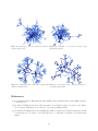
We have implemented the Extract algorithm and produced several examples using both the simple [L, G]
partition and the [T, L, C, S] partition. Figures 6 - 9 are the grid and hypercube examples described in
Section 5.1. In these figures, the edges in L are drawn in darker blue (or black), and the edges of G in red
(or gray).
Jerry Grossman [18] has graciously provided data from a collaboration graph of the second kind, where
each vertex represents an author and each edge represents a joint paper with two authors. The graph in
figures 12 and 13 is a random induced subgraph on the vertices in the collaboration graph with degree at
least 18. The graph in figures 10 and 11 is a subgraph of a biological network which encodes protein-DNA
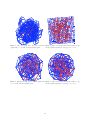
interactions. In these figures, the local edges are drawn in a darker color than the other edges.
12
Figure 6: The grid graph P20 × P20 plus a random Figure 7: The same graph with target lengths set by
graph with p = .1, with all target lengths equal
the Local/Global partition, using (f = 1, ` = 3)
Figure 8: The hypercube Q6 plus a random graph with Figure 9: The same graph with target lengths set by
p = .1, with all target lengths equal
the Local/Global partition, using (f = 6, ` = 3)
13
Figure 10: Subgraph of a biological network, with all Figure 11: Subgraph of a biological network, using
target lengths equal
[T,L,S,C] partition
Figure 12: A subgraph of the collaboration graph, with
all target lengths equal
Figure 13: A subgraph of the collaboration graph, using [T,L,S,C] partition
References
[1] L. A. Adamic and B. A. Huberman, Growth dynamics of the World Wide Web, Nature, 401, September
9, 1999, pp. 131.
[2] W. Aiello, F. Chung and L. Lu, A random graph model for massive graphs, Proceedings of the ThirtySecond Annual ACM Symposium on Theory of Computing, (2000) 171-180.
[3] R. Andersen, F. Chung and L. Lu, Analyzing the small world phenomenon using a hybrid model with
local network flow, Proceedings of the Third Workshop on Algorithms and Models for the Web-Graph
(2004).
14
[4] R. B. R. Azevedo and A. M. Leroi, A power law for cells, Proc. Natl. Acad. Sci. USA, vol. 98, no. 10,
(2001), 5699-5704.
[5] Albert-László Barabási and Réka Albert, Emergence of scaling in random networks, Science 286 (1999)
509-512.
[6] A. Barabási, R. Albert, and H. Jeong, Scale-free characteristics of random networks: the topology of
the world wide web, Physica A 272 (1999), 173-187.
[7] B. Bollobás, Random Graphs, Academic, New York, 1985.
[8] S. Boyles, G. Exoo, On line disjoint paths of bounded length. Discrete Math. 44 (1983)
[9] A. Broder, R. Kumar, F. Maghoul, P. Raghavan, S. Rajagopalan, R. Stata, A. Tompkins, and J. Wiener,
“Graph Structure in the Web,” proceedings of the WWW9 Conference, May, 2000, Amsterdam. Paper
version appeared in Computer Networks 33, (1-6), (2000), 309-321.
[10] K. Calvert, M. Doar, and E. Zegura, Modeling Internet topology. IEEE Communications Magazine,
35(6) (1997) 160-163.
[11] F. Chung and L. Lu, Average distances in random graphs with given expected degree sequences, Proceedings of National Academy of Science, 99 (2002).
[12] Fan Chung and Linyuan Lu, Connected components in a random graph with given degree sequences,
Annals of Combinatorics, 6 (2002), 125-145.
[13] C. Cooper and A. Frieze, On a general model of web graphs, Random Structures and Algorithms Vol.
22, (2003), 311-335.
[14] P. Erdős and T. Gallai, Gráfok előı́rt fokú pontokkal (Graphs with points of prescribed degrees, in
Hungarian), Mat. Lapok 11 (1961), 264-274.
[15] M. Faloutsos, P. Faloutsos, and C. Faloutsos, On power-law relationships of the Internet topology,
Proceedings of the ACM SIGCOM Conference, Cambridge, MA, 1999.
[16] G. W. Flake, R. E. Tarjan, and K. Tsioutsiouliklis, Graph Clustering and Minimum Cut Trees.
[17] N. Garg, J. Konemann, Faster and simpler algorithms for multicommodity flow and other fractional
packing problems. Technical Report, Max-Planck-Institut fur Informatik, Saarbrucken, Germany (1997).
[18] Jerry Grossman, Patrick Ion, and Rodrigo De Castro, Facts about Erdős Numbers and the Collaboration
Graph, http://www.oakland.edu/∼grossman/trivia.html.
[19] A. Itai, Y. Perl, and Y. Shiloach, The complexity of finding maximum disjoint paths with length
constraints, Networks 12 (1982)
[20] S. Jain and S. Krishna, A model for the emergence of cooperation, interdependence, and structure in
evolving networks, Proc. Natl. Acad. Sci. USA, vol. 98, no. 2, (2001), 543-547.
[21] T. Kamada and S. Kawai. An algorithm for drawing general undirected graphs, Information Processing
Letters, 31(1):715, April 1989.
[22] J. Kleinberg, The small-world phenomenon: An algorithmic perspective, Proc. 32nd ACM Symposium
on Theory of Computing, 2000.
[23] J. Kleinberg, S. R. Kumar, P. Raghavan, S. Rajagopalan and A. Tomkins, The web as a graph: Measurements, models and methods, Proceedings of the International Conference on Combinatorics and
Computing, 1999.
15
[24] S. R. Kumar, P. Raghavan, S. Rajagopalan and A. Tomkins, Extracting large-scale knowledge bases
from the web, Proceedings of the 25th VLDB Conference, Edinburgh, Scotland, 1999.
[25] K. J. Lang, Finding good nearly balanced cuts in power law graphs, Preprint 2004.
[26] L. Lovász, V. Neumann-Lara, M. Plummer, Mengerian theorems for paths of bounded length, Periodica
Mathematica Hungaria 9 (1978)
[27] M. E. J., Newman, The structure of scientific collaboration networks, Proc. Natl. Acad. Sci. USA, vol.
98, no. 2, (2001), 404-409.
[28] S. C. North, Drawing graphs with NEATO, NEATO User Manual, April 26, 2004
[29] S. Plotkin, D. B. Shmoys, and E Tardos, Fast approximation algorithms for fractional packing and
covering problems, FOCS 1991, pp. 495–504.
[30] D. J. Watts and S. H. Strogatz, Collective dynamics of ‘small world’ networks, Nature 393, 440-442.
16