Download Los Alamos

LAUR 95−2986
Manual
GMV
Version 2.9
General Mesh Viewer
User’s Manual
By Frank A. Ortega
Los Alamos
NATIONAL
LABORATORY
Los Alamos National Laboratory is operated by the University of California for
the United States Department of Energy under contract W−7405−ENG−36
Edited by Patricia W. Mendius, Group CIC−1
An Affirmative Action/Equal Opportunity Employer
This report was prepared as an account of work sponsored
by an agency of the United States Government. Neither The
Regents of the University of California, the United States
Government nor any agency thereof, nor any of their employees,
makes any warranty, express or implied, or assumes any
legal liability or responsibility for the accuracy, completeness,
or usefulness of any information, apparatus, product, or
process disclosed, or represents that its use would not infringe
privately owned rights. Reference herein to any specific
commercial product, process, or service by trade name,
trademark, manufacturer, or otherwise, does not necessarily
constitute or imply its endorsement, recommendation, or
favoring by The Regents of the University of California, the
United States Government, or any agency thereof. The views
and opinions of authors expressed herein do not necessarily
state or reflect those of The Regents of the University of
California, the United States Government, or any agency
thereof.
Table of Contents
1.0 Getting to Know GMV
1.1 Starting GMV
1.2 The GMV Temporary Field Files
1.3 The GMV User Interface
The mouse controls
Using menus
Buttons
Slider Bars
Scroll bars
1.4 The Main GMV Window
The menu bar
Twist, elevation, and azimuth
Axes orientation viewbox
Magnification slider
1.5 The File Selection Menu
1.6 The GMV Resource file, gmvrc
gmvrc keywords
Sample gmvrc file
2.0 The File Menu
2.1 Read GMV File
New Simulation
Same Simulation
Same Simulation, Same Cells
Auto Read − Same Simulation
Auto Read − Same Simulation, Same Cells
2.2 Put and Get Attributes
2.3 Save gmvrc
2.4 Snapshot
2.5 Quit
3.0 The Display Menu
3.1 Nodes
Viewing nodes, their vectors, and numbers
Vectors
Selecting nodes to display
Selecting nodes by Materials and Flags
Selecting nodes by Node Field Data Range
1−1
1−1
1−1
1−2
1−2
1−2
1−3
1−5
1−5
1−5
1−5
1−5
1−5
1−6
1−6
1−8
1−8
1−9
2−1
2−1
2−1
2−1
2−1
2−2
2−3
2−4
2−4
2−4
2−5
3−1
3−1
3−1
3−2
3−3
3−3
3−4
3.2
3.3
3.4
3.5
Selecting nodes by Search Sphere
Selecting nodes by Number(s)
Selecting nodes by Search Box
Selecting nodes by Groups
Activating node selection
Cells
Viewing cell faces, edges, and numbers
Coloring cells by materials, fields, and flags
Cell vectors
Face vectors
Selecting cells to display
Explode
Polygons
Shading and outlining polygons
Selecting materials to display
Changing explode percentage
Selecting a polygon subset
Changing material order
Tracers
Methods of displaying tracers
Selecting data field for tracer to represent
Selecting tracers to display
Display tracer history
Surfaces
Viewing surface faces, edges, and numbers
Coloring surfaces by materials, fields, and flags
Surface vectors
Selecting surfaces to display
Explode
4.0 The Calculate Menu
4.1 Average
Selecting weighting field
Selecting a field to Average
4.1 Cutlines
Selecting a cutline
Creating a cutline
Cutline display options
Cutline 2D plot
4.2 Cutplanes
Main Cutplanes Menu
Value
3−5
3−5
3−6
3−6
3−6
3−7
3−7
3−8
3−8
3−8
3−8
3−9
3−10
3−10
3−10
3−11
3−11
3−11
3−12
3−12
3−13
3−13
3−14
3−14
3−15
3−15
3−16
3−16
3−16
4−1
4−1
4−1
4−1
4−1
4−2
4−2
4−3
4−3
4−3
4−4
4−4
Node or Cell Field
New Field
Apply Field Change
Cutplane Selection Buttons
Cutplane Description Menu
Clip on Field Subset and Cell Selection
Cutplane Options
Faces
Coutour Lines
Edges
Height
Distance
Adding a cutplane to the main viewer
Adding a cutplane the easy way
4.3 Cutspheres
4.4 Distance
4.5 Field Calc
Selecting a field to build
Build (calculate) the new field
4.6 Grid Analysis
Selecting cells by nodes or cell numbers
Color By:
Median and Voronoi mesh
4.7 Isosurfaces
Adding a material isosurface
Adding a field isosurface
Clip on field subset and cell selection
Coloring isosurfaces with field values
4.8 Isovolume
4.9 Query Data
Getting node and cell values
Probing node and cell numbers
Getting node numbers by field value
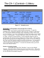
5.0 The Ctl−1 (Controls−1) Menu
5.1 Animation (ortho. and perspective modes)
Number of animation frames
Rotation
Center translation
Magnification
Vector flow
Cutplane
4−4
4−5
4−5
4−5
4−6
4−6
4−6
4−6
4−7
4−7
4−7
4−7
4−8
4−8
4−9
4−9
4−9
4−9
4−9
4−10
4−11
4−12
4−12
4−12
4−12
4−13
4−15
4−15
4−15
4−16
4−16
4−16
4−17
5−1
5−1
5−1
5−2
5−2
5−2
5−2
5−3
Fade
Explode during animation
Snapshot
Quick look
Isosurface animation
Cutsphere animation
5.2 Animation (flight mode)
Setting control points
Saving and Retrieving control points
Quick look and snapshot
5.3 Axes
5.4 Beep Sound
5.5 Bounding Box
5.6 Center
Center on node or cell
5.7 Clip
5.8 Color Bar
Turning on
Preferences
5.9 Color Edit
Materials, Isosurfaces, Isovolume
Changing material or isosurface colors
Reinstating default colors
Field data colormap
Background Color
5.10 Contour Levels
6.0 The CTL−2 (Controls−2) Menu
6.1 Cycle
6.2 Data Limits
Fields
Tracers
6.3 Distance Scale
6.4 Interactivity
6.5 Light
6.6 Line Width
6.7 Point Size
6.8 Plot Box
6.9 Scale Axes
7.0 The CTL−3 (Controls−3) Menu
7.1 Subset
5−3
5−4
5−5
5−5
5−6
5−7
5−8
5−8
5−9
5−9
5−9
5−9
5−9
5−10
5−11
5−11
5−12
5−12
5−12
5−12
5−13
5−14
5−14
5−14
5−15
5−15
6−1
6−1
6−1
6−1
6−2
6−2
6−3
6−3
6−3
6−4
6−4
6−5
7−1
7−1
Nodes, cells, tracers
Polygons
7.2 Texture smoothing
7.3 Time
7.4 Title
7.5 Use Display List
7.6 Vector Control
7.7 Virtual Trackball
7.8 Window Size
7.9 Zoom (Rubberband)
7−1
7−1
7−1
7−2
7−2
7−2
7−3
7−3
7−3
7−4
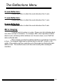
8.0 The Reflections Menu
8−1
8.1 Reflecting about an axis
8−1
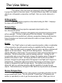
9.0 The View Menu
9.1
9.2
9.3
9.4
9.5
Orthographic
Perspective
Flight
Stereo Perspective
Stereo Flight
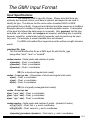
10.0 The GMV Input Format
10.1 Input Specifications
10.2 Input Data Details
Header
Nodes
Nodev
Cells
Vaces
Faces
Nodeids
Cellids
Faceids
Materials
Velocities
Variables
Subvars
Flags
Polygons
Tracers
Tracerid
Problem Time
9−1
9−1
9−1
9−1
9−1
9−2
10−1
10−1
10−9
10−9
10−10
10−10
10−10
10−11
10−11
10−12
10−12
10−12
10−12
10−12
10−13
10−13
10−13
10−14
10−14
10−14
10−14
Cycle Number
Surfaces
Surface Materials
Surface Velocities
Surface Variables
Surface Flags
Surfids
Element groups
Comments
Codename, Codever, Simdate
10.3 Reading some GMV data from a different file
10.4 Sample Input Data
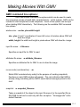
11.0 Making Movies With GMV
11.1 GMV Command Line Options
11.2 GMV Movie Utility
12.0 GMVBATCH
12.1 GMVBATCH − Off screen rendering
12.2 GMVBATCH Command Line Options
13.0 Helpfull Hints
10−14
10−14
10−15
10−15
10−15
10−15
10−15
10−15
10−16
10−16
10−16
10−17
11−1
11−1
11−3
12−1
12−1
12−1
13−1
Illustrations Listing
1−1
1−2
1−3
1−4
1−5
1−6
1−7
2−1
2−2
2−3
3−1
3−2
3−3
3−4
3−5
3−6
3−7
3−8
3−9
3−10
3−11
3−12
3−13
3−14
3−15
3−16
3−17
3−18
3−19
4−1
4−2
4−3
4−4
4−5
4−6
4−7
4−8
4−9
Mouse button schematic
Main GMV window
Main GMV window continued
Twist, Elevation, & Azimuth controls
Axes view box
Magnification & Interactivity controls
The File Selection menu
Auto Read menu
Auto Snapshots menu
SnapShot menu
Nodes menu
Node Field Selection menu
Build Vector submenu
Node Select submenu
Node Materials and Flags submenu
Node Field Data Range submenu
Node Search Sphere submenu
Node Number submenu
Node Search Box submenu
Cells menu
Cell Color By submenu
Cell Materials and Flags submenu
Cell Explode submenu
Polygons menu
Polygon Subset submenu
Material Order submenu
Tracers menu
Tracer Select menu
Surface menu
Average menu
Cutline Selection menu
Create cutline menu
Main Cutplanes menu
Cutplane menu
Cutplane Options menu
Field Calc. Selection menu
Field Calc. Build menu
Grid Analysis menu
4−10
4−11
4−12
4−13
4−14
4−15
5−1
5−2
5−3
5−4
5−5
5−6
5−7
5−8
5−9
5−10
5−11
5−12
5−13
5−14
5−15
5−16
6−1
6−2
6−3
6−4
6−5
6−6
6−7
7−1
7−2
7−3
7−4
7−5
10−1
11−1
Material Isosurface menu
Isosurface demo
Field Isosurface menu
Isovolume menu
Query Data menu
Get Node by Field Value menu
Animation menu
Cutplane Animation submenu
Fade Animation submenu
Explode Animation submenu
Isosurface Animation submenu
Cutsphere Animation submenu
Flight Animation menu
Bounding Box menu
Center menu
Center on node menu
Clip slider controls
Color Bar
Materials, Isosurfaces,
Isovolume color edit menu
Field Colomap Selection menu
Background Color menu
Contour Levels menu
Data Limits menu
Interactivity menu
Light Control menu
Line Width menu
Point Size menu
Plot Box menu
Scale Axes menu
Subset menu
Title menu
Vector Control menu
Window Size menu
Zoom (Rubberband) menu
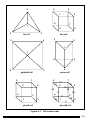
Cell vertex order
GMV Movie menu
0−1
Preface
Revision Record for GMV:
Revision/Date:
Description:
January 2002
Version 2.9
Description and Intent:
This manual describes the General Mesh Viewer (GMV).
GMV is a three−dimensional visualization tool that can process data from any 3−D
mesh. Data to be visualized are taken from a properly formatted input file and
displayed on the screen. With simple pull down menus, windows, and mouse
controls, many special functions are available to maximize the practical value of any
simulation GMV may be asked to visualize.
This manual has three purposes: to teach the beginner how to operate in the GMV
environment, to act as a reference guide for the more experienced user, and to
define the format for the GMV input file.
The only possible prerequisite for the use of GMV is the knowledge of a computer
programming language so that you can write code to generate GMV input data.
However, finished input files are not very difficult to obtain and can also be written
manually using a text editor.
Syntax Conventions:
Words enclosed in double quotes ("like this"), unless otherwise stated, are actual
quoted material from the GMV environment, such as menu options or error
messages. This punctuation does not apply to the description of the GMV input
format. The GMV input file section has its own set of conventions.
0−2
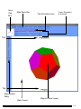
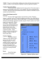
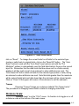
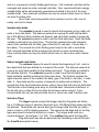
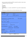
Getting to Know GMV
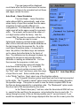
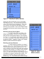
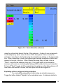
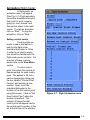
Left mouse button
Right mouse button
Use for selection and rotation
Use for magnification
Middle mouse button
Use to pan
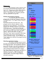
Figure 1−1. Mouse
button schematic
Starting GMV:
To start GMV, the location of the executable must be known. If GMV is in
the current path, simply type:
gmv
on the console and press the enter key. The main GMV window will appear first,
followed by a File Selection menu requesting the name of a GMV input file. Double
click on the name of an input file, or select the file and click on "OK." If the requested
file is not a valid GMV input file, then a box stating this fact will appear and allow you
another chance to select a valid GMV input file. After the file is chosen, the mouse
pointer will change into a watch, indicating that GMV is processing the input file and
preparing to display the data on the screen. Be patient, this may take a few seconds
or even minutes depending on the size of the input file. An object will then be
displayed on the screen. The object displayed depends on the input data and the
following order: polygons, cells, nodes. If polygons exist, they are drawn first. If no
polygons exist, then cells are drawn. If no cells exist, then nodes are drawn, which
must exist in a valid input file. In addition, the "Display" window corresponding to
whatever was displayed first will pop up. For example, if the input file contains
polygon data, the "Polygons" window will automatically pop up when the input file is
first opened.
The GMV temporary field files:
Upon the opening of any input file, GMV creates temporary files on the
local system which hold node field data, cell field data, and polygon data . These
files are not visible to the user. GMV will first attempt to place these files in the
1−1
directory specified in the environment variable "TMPDIR." Set this directory with
the C shell command:
setenv TMPDIR directory_name
where directory_name is the path where you want GMV to place the field data file.
If "TMPDIR" is undefined, GMV will attempt to put the field data file in "/usr/tmp."
These temporary files are removed when GMV ends.
The GMV user interface:
The mouse controls
The mouse controls for GMV have been designed for maximum ease of
use with a three button mouse, (see Fig. 1−1). The left mouse button has two
different functions, depending on whether the cursor is in a menu area or the
viewing area. In the case when the mouse pointer is in the menu area, the left
mouse button is used to pull down menus, select options, drag slider bars, etc.
When the mouse pointer is in the viewing area, the left mouse button functions as a
rotation device. For example, (assuming twist is set to zero) while holding down the
left mouse button and dragging left or right, the object in the viewing area rotates
either left or right, depending on the current orientation of the axes. Moving the
mouse up and down in this manner rotates the object either up or down, again
depending on the current placement of the axes. The middle mouse button
provides a panning function. Holding the middle button and moving the mouse
shifts the object linearly in any direction without any rotation. For example, while
holding down the middle mouse button and dragging right, the object moves to the
right. Finally, the right mouse button is used for controlling the magnification of the
object in the main viewer. For example, while holding down the right mouse button
and dragging up, the object grows larger. Dragging down causes the object to
appear smaller. Motion to the left or right does nothing.
Using menus
The top row of the GMV window is lined with various menus. To open a
menu, click the left mouse button on the name of the menu desired. A small box
will appear with menu options. To select a menu option, again click the mouse on
the desired option. Some of the menu options will open sub menus for specific
program functions which require additional information. To choose from a
submenu, click on the original option and move the mouse to the right and follow
the usual rules for choosing from menus.
1−2
Buttons
GMV has three different types of buttons which are used to select
various functions: regular buttons, toggle buttons, and radio buttons. Regular
buttons are fairly large and have labels inside such as "CLOSE" or "CANCEL." To
activate these, just click the mouse on the button desired. It will temporarily depress
to indicate that it has been activated. The toggle buttons used in GMV are small and
square in shape with labels next to them. These buttons have two different states,
on or off. The little indented square will appear yellow when it is on, and grey when
it is off. Radio buttons are a set of toggle buttons that allow only one selection of the
set and are diamond shaped.
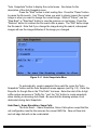
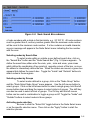
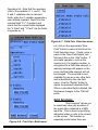
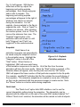
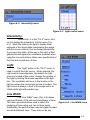
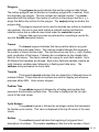
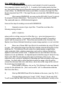
Figure 1−2. Main GMV window
1−3
Axes
View
Box
Main Menu Bar
File Information Line
Twist, Elevation,
& Azimuth
Title
Title
Magnification
Slider
Main Viewer
Object in Main Viewer
1−4
Slider bars
Slider bars are control devices used throughout the GMV user interface.
The use of slider bars is very easy. Just click and hold the left mouse button on the
rectangular shaped slider control and drag it back and forth until the desired
adjustment has been made. When more precise changes are desired, you can
click the left mouse button on a portion of the slider bar not covered by the slider
control and the slider will move at predetermined units.
Scroll bars
Many menus within the GMV environment contain lists of things to
choose from. Lists are placed into scroll boxes. On the right side of a scroll box is
the scroll bar. The scroll bar is much like a slider bar. To scroll through a list, click
and drag the slider back and forth in its track until the desired part of the list is in
view. You may also click in the scroll bar’s track on either side to move through the
list more slowly.
The main GMV window: (see Fig. 1−2 & 1−3)
The menu bar
The menu bar is located at the very top of the main GMV window. The
menu names listed in order are: file, display, calculate, ctl−1 (controls−1), ctl−2
(controls−2), ctl−3 (controls−3), reflections, and view.
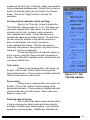
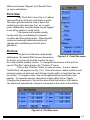
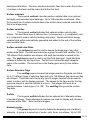
Figure 1−4. Twist, elevation, & azimuth controls
Twist, elevation, and azimuth
These three slider bars are located above the main viewer and control the
viewing angle, (see Fig. 1−4). "Azimuth" is the angle on the X−Y plane measured
from the X−axis. It has the same effect as using the left mouse button and moving
left and right. "Elevation" is the angle in the direction of the Z−axis measured from
the X−Y plane. It has the same effect as using the left mouse button and moving up
and down. The "Twist" adjustment cannot be done with the mouse. The twist slider
rotates the object about the X−axis.
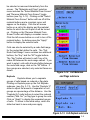
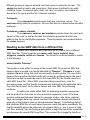
Axes orientation view box
This box is located up and to the left of the light source box, (see Fig.
1−5). The box shows the orientation of the X, Y, and Z axes at all times, even if the
1−5
Figure 1−5. Axes view box
Figure 1−6.
Magnification
control
axes in the main viewer are turned off. It is used mainly for reference.
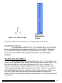
Magnification slider bar
The magnification slider bar (Fig. 1−6) is labeled "Mag" on the top and
has the magnification factor displayed at the bottom (1.00 is default). Sliding the
bar up and down changes the size of the object in the main viewer. The same
effect can be accomplished with the right mouse button, (see The mouse
controls).
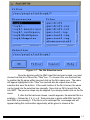
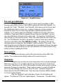
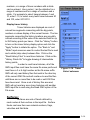
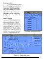
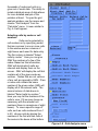
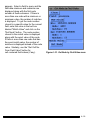
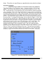
The File Selection Menu:
GMV opens with a File Selection Menu (see Fig. 1−7). Use this menu
to select a file to process. Near the top of the window is a box labeled "Filter." The
filter controls what type of files will be displayed in the "Files" box below. For
example, a filter such as "/usr/people/guest/*.inp" would display only files in the
directory /usr/people/guest that have the extension ".inp". A filter is very useful for
sorting GMV input files from the other files in that particular directory. Clicking on
the "Filter" button near the bottom of the window activates the current filter.
Pressing "Enter" on the keyboard while the mouse pointer is in the filter box has the
same effect.
1−6
Figure 1−7. The File Selection menu
Once the directory with the GMV input file has been located, you must
choose from the list of files in the "Files" box. To choose a file, use the scroll bar
to position the file name within view and click on the file’s name once. The name
will appear highlighted in the "Files" box and will also be copied down to the
selection box near the bottom. If the exact location of the file is known, the name
can be typed into the selection box manually. Now click on OK to launch the file
into GMV. The previous steps may be skipped if you simply double click on the file
name.
If, after the file has been chosen, a watch appears, the selected file is a
pointsize − followed by 2, 4, 6, or 8. Sets point size in pixels.valid GMV input file
and GMV is processing it. If the file is not a valid input file, a message box will
appear stating this, and another opportunity will be given to choose a file.
1−7
The GMV resource file, gmvrc:
The file gmvrc is a GMV resource file that contains a set of generic
drawing instructions that affect the initial display of a simulation. When the first
input file is read, or when a file for a new simulation is read, GMV will look for the
gmvrc file in the directory where GMV is started. If gmvrc is not found in the current
directory, then GMV will look for gmvrc in the user’s home directory. If a gmvrc file
is found, then the display command settings in gmvrc will override the display
defaults. Note that if a gmvrc command asks to display an object that does not
exist, then the display may be blank. For example, if gmvrc asks for polygons to be
displayed and polygons do not exist, then the image will be blank.
gmvrc keywords
The drawing options available in gmvrc are all keyword driven. The
keywords and their options are:
gmvrc − indicates the start of a gmvrc file, required.
azim − followed by a floating point number between −180 and 180. Sets the
azimuth
angle.
elev − followed by a floating point number between −180 and 180. Sets the
elevation
angle.
twist − followed by a floating point number between −180 and 180. Sets the twist
angle.
mag − followed by a floating point number. Sets the magnification.
nodes − followed by on or off. Sets nodes display on/off.
nodenumbers − followed by on or off. Sets node numbers display on/off.
cellfaces − followed by on or off. Sets cell faces display on/off.
celledges − followed by on or off. Sets cell edges display on/off.
cellnumbers − followed by on or off. Sets cell numbers display on/off.
polygons − followed by on or off. Sets polygons display on/off.
polygonlines − followed by on or off. Sets polygon lines display on/off.
axis − followed by on or off. Sets axis on/off.
time − followed by on or off. Sets time on/off.
cycle − followed by on or off. Sets cycle on/off.
linesize − followed by 1, 2, or 3. Sets line width in pixels.
linetype − followed by regular or smooth. Sets line type.
pointsize − followed by 2, 4, 6, or 8. Sets point size in pixels.
pointshape − followed by square or round. Sets point shape.
ncontours − followed by a positive integer. Sets the number of contour levels.
xreflect − followed by on or off. Sets reflection about x axis on/off.
yreflect − followed by on or off. Sets reflection about y axis on/off.
1−8
zreflect − followed by on or off. Sets reflection about z axis on/off.
xscaleaxis − followed by a positive floating point number. Sets the scale factor in
the x direction.
yscaleaxis − followed by a positive floating point number. Sets the scale factor in
the y direction.
zscaleaxis − followed by a positive floating point number. Sets the scale factor in
the z direction.
boundingbox − followed by on or off. Sets bounding box on/off.
boundingboxcoords − followed by on or off. Sets bounding box coordinates on/off.
background_red − followed by a positive floating point number between 0 and 1.
Sets the red component of the background color.
background_green − followed by a positive floating point number between 0 and 1.
Sets the green component of the background color.
background_blue − followed by a positive floating point number between 0 and 1.
Sets the blue component of the background color.
display_list − followed by on or off. Sets display list on/off.
trackball − followed by on or off. Sets the virtual trackball on/off.
beepsound − followed by on or off. Sets the GMV beep sound on/off.
distscale− followed by on or off. Sets the distance scale on/off.
windowwidth − followed by a positive integer. Sets the window width.
windowheight − followed by a positive integer. Sets the window height.
textureflag− followed by on or off. Sets texture smoothing on/off.
attributes − followed by a gmv attributes file filename. Specifies an attributes file to
read for initial image.
end_gmvrc − indicates the end of the gmvrc file, required.
These keywords all have functional interactive counterparts that are available via
menus and should be recognizable. Note that gmvrc and end_gmvrc are the only
required keywords, all others are optional. If GMV encounters the attributes
keyword, and the file does not exist, then it is ignored. Fully qualified attributes
filename must be specified if the attributes file is not in the current directory.
Placement of the attributes keyword in gmvrc is important, attributes will override
previous options, while subsequent gmvrc options will override attributes. The best
way to create a gmvrc file is to have GMV generate one for you with the "Save
gmvrc" option in the "Files" menu A gmvrc file will be generated with the options set
to those used by the current image.
Sample gmvrc file
gmvrc
azim −120.000000 elev 20.500000 twist 0.000000
mag 1.000000
nodes off nodenumbers off
1−9
cellfaces off celledges off cellnumbers off
polygons on polygonlines off
axis off time off cycle off
linesize 1 linetype regular
pointsize 2 pointshape round
ncontours 10
xreflect off yreflect off zreflect off
xscaleaxis 1.000000 yscaleaxis 1.000000 zscaleaxis 1.000000
boundingbox on boundingboxcoords off
background_red 1.000000 background_green 1.000000
background_blue 1.000000
end_gmvrc
1−10
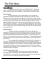
The File Menu
Read GMV file:
The first option in the "File" menu is "Read GMV File." Choose this
option, and a pull down menu will appear. The pull down menu contains three
options: New Simulation, Same Simulation, and Auto Read − Same Simulation.
New Simulation
The New Simulation option enables GMV to read a file that was
generated by a different simulation than the simulation that created the current
GMV input file. Selecting this option will display the File Selection menu (see Fig.
1−10) to select the next input file. Then the current custom menus will be destroyed
while new custom menus for the data on this input file will be created. The first
image will display either nodes, cells, or polygons following the rules used when
GMV is started (see Chapter 1). Only the view angles, magnification, and material
colors will be the same as the last image from the previous GMV file. The 3−D plot
box, the subset ranges, and the field data ranges will all be reset to reflect the data
in the new GMV file.
Same Simulation
The Same Simulation option allows GMV to read a file that was
generated as a different time step from the same simulation as the simulation that
created the current GMV input file but with a different cell configuration. Selecting
this option will display the File Selection menu (see Fig. 1−10) to select the next
input file. The current custom menus are not destroyed . The image displayed after
reading the input file will contain exactly the same attributes as the image from the
previous file.
The new image will be displayed much faster after the file is read since
the custom menus do not have to be recreated. Also, any cutlines, cutplanes,
isosurfaces, and isovolumes that existed in the previous image will be automatically
calculated and displayed. The 3−D plot box, the subset ranges, and the field data
ranges remain the same for successive implementations of the Same Simulation
read option unless manually reset, an attributes file is read, or until a file is read with
the New Simulation read option.
Same Simulation, Same Cells
The Same Simulation, Same Cells option is similar to the Same
Simulation option, except that the cell configuration must be the same as the
current GMV file. In other words, the cells must contain the same node numbers. A
new cell face list and cell edge list will not be recalculated.
2−1
The new image will be displayed
much faster after the file is read since the custom
menus do not have to be recreated and cell faces
and edges remain the same.
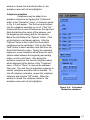
Auto Read − Same Simulation
The Auto Read − Same Simulation
option allows GMV to automatically read a time
series family of input files created from the same
simulation but with possibly different cell
configurations. The filenames to be read by this
option must all be the same except for a numeric
suffix. The numeric suffix must all be either a 3
or 4 digit number within the family. Also the
current GMV file must be a member of the family.
The files are read in a user
determined sequence and the image produced
after a file is read will have the same attributes as
the last image from the previous file. As in the
read Same Simulation option, it is important to
have the plotbox, field data range, and subsets
set to values that reflect data for the family of
files. The attributes can be changed, however, by
pausing the sequence and manually setting
attributes or reading an attributes file. You can
then resume the sequence or start over.
Selecting this option will display the
Auto Read menu (see Fig. 2−1), unless the
current file does not contain a numeric suffix. In
the "First": and "Last:" text boxes, enter the range
Figure 2−1. Auto Read Menu
of input files to read. Enter a stride (skip value)
in the "Stride:" text box. Next, select one of the direction options.
The "Forwards" direction option reads files form first to last incremented
by the stride. The "Forward to Latest" option looks for the latest existing file within
the specified range. This option is useful to view the latest complete GMV file as
the files are being generated by a simulation code. The "Backwards" option reads
files from last to first decremented by the stride.
In the "Search time (sec):" text box, enter the time interval GMV will use
to search for the next file in the sequence, not including the time to read a file. To
sweep through a series of files as fast as possible use a 1 second interval If you
would like snapshots of the first image displayed after the next file is read, press the
2−2
"Auto Snapshots" button to display the control menu. See below for the
description of the Auto Snapshot menu.
Press the "Start" button to start reading files. Press the "Pause" button
to pause the file search. Use "Pause" when you want to closely inspect the current
image or when you want to change the current image. While in "Pause", use the
"Step Back" or "Step Next" button to view the previous or next image. Press the
"Resume" button to continue the file search after a pause. The "Quit" button stops
the file search. Note that if you change the image during the search, subsequent
images will use the image attributes of the image you changed.
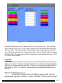
Figure 2−2. Auto Snapshots Menu
To automatically create a snapshot from each file, press the "Auto
Snapshots" button and the Auto Snapshots menu appears (see Fig. 2.2). Enter the
file prefix for the rgb files in the "File Prefix" text area. Enter the start of the 4 digit
suffix number sequence in "Suffix No.:" and the "On" button to create snapshots
when starting or resuming Auto Read. Be sure that the drawing window is not
obstructed during Auto Snapshots.
Auto Read − Same Simulation, Same Cells
The Auto Read − Same Simulation, Same Cells option except that the
cell configuration must be the same as the current GMV file. New cell face lists
and cell edge lists will not be recalculated.
2−3
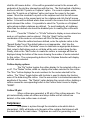
Figure 2−3. SnapShot menu
Put and get attributes:
Attributes are the collective sum of all the options available in GMV,
Normally when GMV is first run, all of GMV’s options are set to their defaults. For
example, the "Twist," "Elevation," and "Azimuth" slider bars are all set to zero and
the magnification factor is set to one. However, suppose you have worked on
viewing the object from a certain angle and have created isosurfaces and a
cutplane, or you want to apply the attributes to a different time step of the same
simulation. If you want these to reappear the next time you start GMV, you can
save the attributes in a file and retrieve them later. Choosing the "Put Attributes"
option brings up a file selection menu. Enter a file name then click OK to save the
file. The "Put Attributes" function is necessary in order to create time sequence
movies of a simulation (See The GMV Movie utility). The attribute file may be
retrieved later by invoking the "Get Attributes" option under the "File" menu. Take
note that when a set of attributes is saved and then immediately retrieved, the name
of the attribute file will not show up in the "Get Attributes" list of files until the "Filter"
button is clicked, updating the file list.
Save gmvrc:
Save gmvrc will save a gmvrc file in the directory where GMV was
started. The current generic display options will be saved in gmvrc.
Snapshot:
Snapshot is a tool that can create image files of the currently displayed
GMV data, (see Fig. 2−3). A GMV snapshot can only be two sizes: full size and
movie size. Movie size (720 x 486) is the smaller one and can be used to create a
sequence of images for animation. There is also an option to create a PostScript
file of only lines (Display List must be off for PS Lines). Snapshot images are
always saved in the SGI−RGB format. There are many freeware utilities available
to convert to other formats.
After the "Snapshot" option has been chosen, a small window will
appear. "Full Size and "PS Lines" options appear. Choose one. The radio button
2−4
next to the currently selected snapshot size will be yellow. When all is ready, click
on "Snap" and a File Selection Menu will appear. Enter a file name and click on the
"OK" button to save the snapshot. After the image is stored, click on the "Close"
button and continue work. The snapshot File will be saved in the directory indicated
on the File Selection Menu.
Quit:
Choose this option to quit GMV.
2−5
The Display Menu
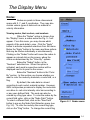
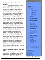
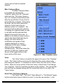
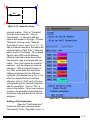
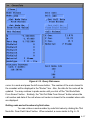
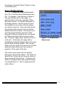
Nodes:
Nodes are points in three−dimensional
space with X, Y, and Z coordinates. They may also
contain various types of data such as material or
velocity information.
Viewing nodes, their vectors, and numbers
When the "Nodes" option is chosen from
the "Display" menu, a nodes menu like Fig. 3−1 will
appear. From this menu, you may choose which
aspects of the node data to view. Click the "Apply"
button to activate requested selections from the menu.
Below the "Apply" button in the menu are three options
that may be chosen individually or simultaneously.
Clicking on the "Nodes" button will cause the nodes to
appear as colored dots on the screen, where the
colors are determined by the "Color By:" options.
Below the "Nodes" button is the
"Numbers" selection box. When this option is
activated, each node’s respective number will be
displayed next to its point on the screen.
Below the "Numbers" button is the "Color
By" section. In this section you choose whether you
want to color the nodes by materials, a node field, or a
flag.
By default, the node data is colored
according to each node’s material number. However,
GMV incorporates provisions to display the node data
as a blue−to−red color intensity color bar according to
or any user−defined field. The node can also be
colored by a flag type value. To color the nodes by the
current field value, click on the "Node Field:" button.
To select a different field, click on the "New Field"
button to pop up the Node Field Selection menu (see
Fig. 3.2). To color the node by the current flag type,
click on the "Flag" button. To change the current flag
Figure 3−1. Nodes menu
3−1
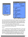
Figure 3−2. Node Field
Selection Menu
Figure 3−3. Build Vector submenu
type, click on the "New Flag" button and select a flag type from the Flag Selection
menu. Nodes can also be colored by groups, if entered. If group color is selected,
only those nodes that are in a group are displayed. Only one of material, node
fields, flags, or groups may be selected at a time. When a node field is selected
to color the nodes, a color bar scale will appear on the far left of the main viewer
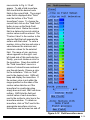
that gives you the range of values in relation to the color bar.
To see any nodes that have a 0 material number, or not in a group,
press the "Show nodes with 0 material nos." button. Any nodes with 0 material
number will have the text color as a material color.
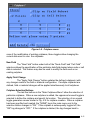
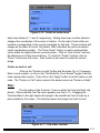
Vectors:
Choose the "Vectors" button to build and draw vectors. To turn on the
vectors, click on the button. A submenu will appear. The menu contains a toggle
button to toggle the vectors on and off. When this button is selected, each node’s
vector data will be displayed according to the current X, Y, and Z components of
the vector. Click Apply on the Nodes menu to activate vectors. The vector is
colored by the "Color By" selection with a tall pyramid as the arrow head. The
base of the arrow head is drawn in the text color to help determine direction.
There is also the "Build Vector" option. Click here and a submenu
3−2
Figure 3−4. Node Select submenu
similar to Fig. 3−3 will appear. With this option, you can tailor the X, Y, and/or Z
components of the vectors to any field; default is the velocity data (U, V, and W).
To change a vector component, click the "New Field" button under the vector
component to change. The Node Field Selection menu is then displayed (see Fig.
3−2). Choose the desired field for that vector component from the list of fields. A
vector component’s current field will be displayed to the right of its name under the
heading "Active Fields". Choose "NONE" to zero out a vector component.
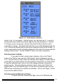
Selecting nodes to display
If you want to select certain nodes to display, click on the "Select"
button in the "Nodes" menu and the "Node Select" menu is displayed (see Fig.
3−4). Use this menu to select nodes by materials and/or flags, by a data range of
a node field, by a search sphere, by node numbers, a search box, or node groups.
To specify a selection type, click on one of the category buttons to bring up a
selection menu. After specifying the selection criteria, click on the "Select On"
toggle button to use the selection type. If more than one selection type is set on,
GMV will use a logical and to combine the selections. Click on the "Apply " button
to process the search criteria.
Selecting nodes by Materials and Flags
To select nodes by materials and flags, click on the "Materials and
3−3
Figure 3−5. Node Materials and Flags submenu
Flags" button and the Node Materials and Flags
Menu appears (see Fig. 3−5).
The available materials will be listed on the left
side of the menu. Following the materials are all
the flag types,if any, followed by the different flag
values. Between each column of selection
criteria are the two logical operators "AND" and
"OR."
Highlight the desired materials, then
highlight the desired flag values.
The "On" and "Off" buttons are used to select or
unselect all of the materials or flags. Next, decide
on the logical operator (and/or) to build a
left−to−right boolean operation.
Selecting nodes by Node Field Data Range
To select nodes by a node field data
range, click on the Node Field Data Range button
and the "Node Field Data Range" menu appears
(see Fig 3−6). Select a field to operate on by
Figure 3−6. Node Field
Data Range submenu
3−4
Figure 3−7. Node Search Sphere submenu
clicking the "New Field" button to pop up the Node
Field Selection menu. The minimum and maximum
values of the field will then be displayed. Then enter
your minimum and maximum data range for node
selection in the text fields. Click on the "Reset" button
to reset the field minimum and maximum values in the
text field.
Selecting nodes by Search Sphere
To select nodes within or outside a user
defined search sphere, click on the "Search Sphere"
button and the "Node Search Sphere" menu appears
(see Fig. 3−7). To define the search sphere, enter the
x, y, and z coordinates of the center of the sphere and
the sphere’s radius. Toggle the "Inside" and "Outside"
buttons to select nodes in those regions.
Selecting nodes by Number(s)
To select nodes by numbers or a range of
numbers, click on the "Node Numbers" button and the
"Node Numbers" menu pops up (see Fig 3−8). The
menu contains 50 lines where individual node numbers,
a range of node numbers, or a range of node numbers
with a stride can be entered (one entry per line). A
colon (:) is used as the delimiter when defining a range
of numbers or a range of numbers with a stride. The
format used to define a range of node numbers is
first:last, e.g. 1:10. The format used to define a range
Figure 3−8. Node
Number submenu
3−5
Figure 3−9. Node Search Box submenu
of node numbers with a stride is first:last:stride, e.g. 20:100:10. All node numbers
must be greater than 0, and any number greater than the maximum node number
will be reset to the maximum node number. If a line contains an invalid character,
an error message will appear in the Node Select menu indicating the line number
with the error.
Selecting nodes by Search Box
To select nodes within or outside a user defined search box, click on
the "Search Box" button and the "Node Search Box" (Fig. 3−9)menu appears . To
define the search box,either enter the xmin, ymin, zmin and xmax, ymax zmax
which define the coordinates of two points at opposite corners of the box, or move
the sliders to interactively define the box. When the sliders are moved, a green box
appears that defines the search box. Toggle the "Inside" and "Outside" buttons to
select nodes in those regions.
Selecting nodes by Groups
To select nodes defined in a group, click on the "Node Group" button
and the "Node Select Node Group" menu appears . Use the left mouse button to
select groups. Click on the left mouse button to select a single group, hold the left
mouse button down and drag the mouse to select a block of groups. The shift key
can also be used to select a block of groups. The Ctrl key and the left mouse
button can be used in combination to toggle a group on/off. Toggle the "Inside" and
"Outside" buttons to select nodes in those groups.
Activating node selection
Be sure to click the "Select On" toggle button in the Node Select menu
or on the specific selection menu. Then click on the "Apply" button to start the
selection process.
3−6
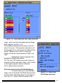
Cells:
Cells are three−dimensional fixed
shapes in space, such as cubes, pyramids, or
prisms. Cells are defined by the nodes at their
vertices in the input file.
Viewing cell faces, edges, and numbers
Choosing the "Cells" option under the
"Display" menu brings up the "Cells" menu, (Fig.
3−10). Here you may choose which aspects of
the cells you wish to view. The "Faces" option
displays the face of the cells as an interpolated
blended color polygon where the colors are
based on the selected cell or node field. If the
cell face is colored by a node field, the
"Contours" option under "Faces" displays contour
lines on the faces. The contour lines are drawn
at the intervals shown on the cells Color Bar.
The "Shaded" option under "Faces" turns on the
lighting model and shades the faces. The
"Refine" option, available only when the cell
faces are colored by a node field, adds an
interpolated point at the face center to provide a
smoother color change across the face. When
the "Test Normals" option is selected, cells with
inward pointing normals will be drawn in black
(outward face normals using the righthand rule is
the standard). The "Edges" option displays the
edges of the cells as a colored wireframe image.
The "Median Mesh Edges" option generates and
displays median mesh edges. If both "Faces"
and "Edges" are selected, the edges are colored
grey. If both "Edges" and Median Mesh Edges"
are selected, cell edges are drawn in black. If
"Faces", "Edges", and Median Mesh Edges" are
selected, the median mesh is drawn in white.
The "Cell Numbers" option draws the cell number
at the center of the cell in the edge color for the
cell while the "Node Numbers" option draws the
cell’s node numbers in the text color and the
"Face Numbers" option draws the cell’s face
Figure 3−10. Cells menu
3−7
numbers in the text color. Cell faces, edges, and numbers
may be displayed simultaneously. Simply click on the box
next to the desired option just as is done in the "Nodes"
menu. Click on the "Apply" button to activate the
selections.
Coloring cells by materials, fields, and flags
Click on the "Color By:) button to display the
"Cell Color By" submenu (see Fig. 3−12). Cell edges are
colored by material color, flag values, or a blue−to−red
intensity color for cell− centered, node−centered or
face−centered field values. If node field values are
selected the edges are smoothly colored. The cell faces
can be colored by material or flag values as well as a
blue−to−red intensity color of cell−centered or
node−centered field values. Cell faces can also be
colored by cell groups or face groups, only cells or faces
that are in a group are displayed.
To see cells that have a 0 material number, or
not in a group, press the "Show cells with 0 material no."
button. Any cells with 0 material number will have the text
color as a material color.
Cell vectors
If there is cell−centered data, cell vectors can
be built. Click on the "Vectors" button to bring up the
appropriate submenu. The procedure to display and build
vectors is the same as node vectors.
Figure 3−11. Cell
Color By submenu
Face vectors
If there is face−centered data, cell vectors can
be built. Click on the "Vectors" button to bring up the
appropriate submenu. The procedure to display and build
vectors is the same as node vectors. Face vectors are
drawn in a grey color.
Selecting cells to display
This is done in the same manner as described
in the previous section about nodes and their materials
and flags, cell field range, search sphere, cell number(s),
search box, and cell groups. Additionally, materials can
3−8
be selected or removed interactively from the
screen. The "Materials and Flags" selection
menu includes the "Select Material From Screen"
and "Remove Material From Screen" toggle
buttons (see Fig. 3−12). Clicking on the "Select
Material From Screen" button will turn off all the
material buttons and a crosshair cursor will
appear on the display. Click the left mouse
button on a cell in the display and the material
button for which the cell is part of will be turned
on. Clicking on the "Remove Material From
Screen" button will display a crosshair cursor.
Click the left mouse button on a cell to turn off its
material button. As before press the "Apply"
button to display the selected cells.
Cells can also be selected by a node field range
for the nodes that define the cells. The "Cell
Node Field Range" menu contains two additional
buttons, the "Any" and the "All" toggle buttons.
The "Any" button will select a cell if any of its
nodes fall between the node range valued. If you
want to select cells with all nodes falling between
the node field range, click on the "All" button. If
face groups are selected, only selected faces are
drawn.
Explode
Figure 3−12. Cell Materials
and Flags submenu
Explode allows you to separate
groups of cells based on material or flag data.
Clicking on Explode pops up the Cell Explode
submenu, (see Fig. 3−13). Use the "Explode %"
slider to adjust the amount of separation of cell
groups as a percentage of the distance. Use the
"Explode On" radio buttons to select the material
number ("Mat. No") or flag type to group the cells.
Click on "Apply" to display the separated groups
of cells. To return to the initial setup, return the
slider bar back to zero and press apply.
Figure 3−13. Cell Explode submenu
3−9
Polygons:
The "Polygons" menu is used to view
the surfaces made by the input polygons, (see
Fig. 3−14). Polygons are surface facets that are
shaded according to the location of the light
source. The polygons are colored by material
color as specified in the input file.
Shading and outlining polygons
To change the way GMV displays
polygon data, choose the "Polygons" option from
the display menu. The "Apply" button is used to
activate
the desired selection from this menu. The
polygons can be outlined, shaded, or both,
depending on your preference. The way the
polygons are "Shaded" depends on the location
of the light source. This location of the light
source can be changed by using the light source
box in the upper right corner of the main GMV
window. See the information on page 1−7.
When the "Lines" option is selected, GMV draws
lines between the vertices of the polygon, to
create a wireframe image. If both "Shaded" and
"Lines" options are selected, the polygon lines are
colored white.
Selecting materials to display
The surface materials may be turned
on or off. The materials are listed at the bottom of
the "Polygons" menu. For convenience, there is
an on and off button to turn all the materials on or
off at once. Use the material toggle buttons to
select individual material surfaces for display.
The "Select Material From Screen" and "Remove
Material From Screen" toggle buttons allow
interactive selection as in the Cell Material
selection Menu. Press the "Apply" button to
activate the selection.
Figure 3−14 Polygons menu
3−10
Figure 3−15. Polygon subset submenu
Changing explode percentage
Use the "Explode%" slider to separate surfaces by material, giving an
exploded view of the surfaces.
Selecting a polygon subset
When you click on the button labeled "Subset" in the "Polygons" menu,
a submenu labeled "Polygon Subset" will appear, (see Fig. 3−15). There are six
sliders and six text boxes in the window. These are used to define a polygon
subset region. The minimum and maximum values listed in the six text boxes
define a cube in space. Any polygon that does not lie completely within this cube
will no longer be shown in the main viewer. Use the sliders to modify the polygon
subset cube. A purple bounding box is displayed as the sliders are moved to help
visually set the polygon subset region. Alternatively, a value can be entered in the
text portion of the menu. Press the "Apply" button to initiate the subset. Any
polygon not falling within the new polygon subset region will be erased. Clicking on
the close button will close the subset window, leaving any changes in effect.
Clicking on the Reset button will reset the polygon subset box to the problem size
and all polygons will then be drawn.
Changing material order
The material order function comes into play when two or more polygons
occupy the same region of space. Because only one of the stacked polygons may
be shown at a time, you must decide the order of precedence for the materials so
that GMV will know which polygon to draw. Material order is also important when
more than one material is transparent. Transparent materials must be in a
back−to−front order in order to be drawn correctly. By default, material number 1 is
first, followed by material number 2 and so on.
To change the current material order, click on the button labeled "Mat
Order" in the "Polygons" menu. A submenu similar to Fig. 3−16 will appear. On the
far right you will see the current materials listed in order. To change the order, click
on each material button from the left−hand column in the desired order. The
3−11
Figure 3−16. Material Order submenu
materials will be listed in the middle column in the proposed order. Each material
may be chosen only once. If you make a mistake in the material ordering process,
click on "Undo." This will clear the order listing of materials and allow you to start
over. When the materials are in the desired order, click on "Apply" and the changes
will take effect. The new order number will appear on the right−hand column. Click
on "Close" when finished.
Tracers:
Tracers are points in space used for monitoring data in locations where
nodes do not exist. Tracers are defined by their X, Y, and Z coordinates and by the
data they are assigned by the input file. Tracers can be assigned multiple fields of
data, such as in Fig. 3−17 where it reads pressure and temperature data from the
input file.
Methods of displaying tracers
Tracers can be represented in four different ways by GMV, either as
regular points, big points, numbers, or values. When the "Tracers" menu is brought
3−12
up from the "Display" menu bar, you will notice four
selection boxes under the heading "Draw as."
When the "None" option is chosen, no tracer data
will be shown. The "Regular Points" option displays
tracer data as colored points whose size is
determined by the "Point Size" option in "Controls
2". The "Big Points" option displays tracer data as
large, bright icosahedra centered on the tracer
location. When "Numbers" is selected, the
sequential number of each tracer is displayed.
Do not get the tracer numbers confused with the
node or cell numbers. When all three are displayed
simultaneously, it is hard to tell them apart. Finally,
there is the "Values" option. This one tells GMV to
display the value of each tracer in the correct
location on the screen. Depending on which field is
currently selected, the colors for tracer display are a
blue−to−red intensity color depicting the values of
the field selected for display. Click on the "Apply"
button to activate your selections.
Selecting data field for tracer to represent
A main color bar pops up inside the
GMV main viewer when tracers are displayed. The
tracer always takes on the color of its value in the
currently selected field. The available fields are
listed under the heading "Fields" at the bottom of
the tracer window. To select a field, click on the
radio button next to its name. The colors of the
tracers in the main viewer will change. If the input
file read in by GMV contained no tracer data, then
there will be no fields to choose from in the "Tracers"
menu. Selecting the "Close" button will close the
menu, leaving any changes you have made intact.
Selecting tracers to display
Tracers can be selected for display by
number(s). Click the "Select" button to display the
"Tracer Select Menu" (see Fig. 3−18). As in
selecting nodes or cells by number, there are 50
lines where a tracer number, a range of tracer
Figure 3−17. Tracers menu
3−13
numbers, or a range of tracer numbers with a stride
can be entered. Use a colon (:) as the delimiter for a
range of numbers and for a range of numbers and a
stride. For example to select tracers between 1 and
10, enter 1:10, to select every tenth tracer between 20
and 100, enter 20:100:10.
Display tracer history
Tracer histories are displayed as a set of
colored line segments connecting with the big points,
numbers or values display of the current tracers. The line
segments connecting the history locations are smoothly
colored according to the value of the selected field for up
to 250 history points per tracer. Click the "History" button
to turn on the tracer history display option and click the
"Apply" button to initiate the option. The "Back to" and
"Stride" input areas are used to control the last file to read
and a stride (skip value) between files. Click on the
"Read History Files" to read trace histories. Click on the
"History Points On" to toggle drawing of intermediate
history points.
In order to read trace histories, all of the
GMV input files must have the same file name prefix and
must have a 3 or 4 digit number as the file name suffix.
GMV will only read history files that exist in the directory
of the current GMV file and will continue to read the files
until there are no more files to be read or until 250 files
have been read. Once a set of history files are read,
GMV will not read any more trace histories until another
GMV input file is read using the Read GMV option of the
File menu.
Figure 3−18. Tracer
Select submenu
Surfaces:
Surfaces are sets of facets defined by
mesh nodes at their vertices in the input file. Surface
facets can have their own material numbers, flags,
velocities and field data.
3−14
Viewing surface faces, edges, and
numbers
Choosing the "Surfaces" option
under the "Display" menu brings up the
"Surfaces" menu, (Fig. 3−19) Here you may
choose which aspects of the surfaces you
wish to view. The "Faces" option displays
the surface facet as an interpolated blended
color polygon where the colors are based on
the selected surface or node field. If the
surface face is colored by a node field, the
"Contours" option under "Faces" displays
contour lines on the faces. The contour lines
are drawn at the intervals shown on the
surfaces Color Bar. The "Shaded" option
under "Faces" turns on the lighting model
and shades the facets. The "Refine" option,
available only when the surface facets are
colored by a node field, adds interpolated
points at the facet center and edge centers to
provide a smoother color change across the
facet. The "Edges" option displays the edges
of the surfaces as a colored wireframe
image. If both "Faces" and "Edges" are
selected, the edges are colored grey.. The
"Surface Numbers" option draws the surface
number at the center of the facet in the edge
color for the surface while the "Node
Numbers" option draws the surface’s node
numbers in the text color. Surface faces,
edges, and numbers may be displayed
simultaneously. Simply click on the box next
to the desired option just as is done in the
"Nodes" menu. Click on the "Apply" button to
activate the selections.
Coloring surfaces by materials, fields, and
flags
Surface edges are colored by
material color, flag values, or a blue−to−red
intensity color for surface− centered or
node−centered field values. If node field
Figure 3−19. Surfaces menu
3−15
values are selected the edges are smoothly colored. The surface faces can be
colored by material or flag values as well as a blue−to−red intensity color of
surface−centered or node−centered field values. Surfaces can also be colored by
groups, only surface elements that are in a group are displayed.
To see surfaces that have a 0 material number, or node group, press
the "Show Surfaces with 0 material no." button. Any surfaces with 0 material
number will have the text color as a material color.
Surface vectors
If there is surface−centered data, surface vectors can be built. Click on
the "Vectors" button to bring up the appropriate submenu. The procedure to display
and build vectors is the same as cell vectors.
Selecting surfaces to display
This is done in the same manner as described in the previous section
about cells and their materials and flags, surface field range, node field range,
search sphere, surface number(s), search box, and surface groups.
Explode
An exploded view of surfaces is accomplished just as in cell explode.
3−16
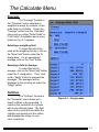
The Calculate Menu
Average:
The "Average" function in
the "Calculate" menu calculates a
weighted average, by material, of two
node fields or cell fields. Chose the
"Average" option from the "Calculate"
menu and select either "Node Fields" or
"Cell Fields" (if available) and a menu
similar to Fig. 4−1 appears.
Selecting a weighting field
To select the field to be
used as the weighting function, click on
the "New Field" button under the W:
designation. For an unweighted
average, click on the "One" button.
Selecting a field to Average
To select the field to
average, click on the "New Field" button
under the F: designation. Then click
on the "Apply" button to generate the
averages. The averages will be
displayed in the scrolling list under the
"Apply" button.
Cutlines:
The "Cutlines" function in
the "Calculate" menu allows up to
twenty cutlines to be generated. A
cutline is the centerline of a cylinder
with a user defined radius. The field
value of any node that lies within the
cylinder is projected onto the cutline
and displayed as a blue−to−red
color−coded line.
Figure 4−1. Average menu
4−1
Selecting a cutline
Choose the "Cutlines" option
from the "Calculate" main menu bar and
a menu similar to Fig. 4−2 will appear.
The numbers are the cutline number
and "NONE" indicates that the cutline
has not been generated. A field name
indicates that a cutline has been
generated for that field. Select one of
the cutlines and a menu similar to Fig.
4−3 will appear.
Creating a cutline
A cutline can be created in
one of five methods. The line can be
defined by entering the x, y, and z
values of the two endpoints of the line.
These can be entered on the two rows
of boxes identified as "P1" and "P2". A
second method is to use the "1 Point"
option. Click on the "1 Point" box then
move the cursor to the main viewer. A
crosshair cursor will appear; place the
cursor on a point on the screen, and
Figure 4−2. Cutline Selection menu
Figure 4−3. Create cutline menu
4−2
click the left mouse button. A line will be generated normal to the screen with
endpoints at the plot box intersections with the line. The third method of defining
the line is with the "2 points on Cutplane" option. If a current cutplane exists,
select the "2 points on a Cutplane" option and move the cursor to the main
viewer. Move the crosshair to a point on the cutplane and click the left mouse
button; then move to the second point on the cutplane and click the left mouse
button. A line will be defined where lines normal to the screen from the selected
points intersect the cutline. It is possible to select the "2 points on a Cutplane"
option when multiple cutplanes are defined. To avoid ambiguity, all cutplanes
other than the desired one should be disabled prior to creating the cutline with
this option.
Press the "2 Nodes" or "2 Cells" buttons to display a menu where tow
node or cell numbers can be entered. Click the "Apply" button and the
coordinates of the nodes or cell centers will fill in the two point values.
When the cutline has been defined, enter the cylinder radius in the
"Search Radius" box if the default radius is not appropriate. Hint: Use the
"Distance" option of the "Calculate" menu to determine an appropriate distance.
Next, select a field whose node or cell data will be color coded along the line.
Finally, click on the "Add" button to create the cutline; a message will then be
displayed along the bottom of the menu showing the number of nodes selected
for this cutline. The corresponding button in the Cutplane Selection will display
the field value selected.
Cutline display options
The "On" button toggles the cutline display for the selected cutline on
or off. The "Nodes" button, when on, displays the nodes selected for the cutline.
The "Nos." button displays the node numbers for the nodes selected for the
cutline. The "Wave" toggle button with its slider is used to display the function
wave of the data along the cutline. Use the wave slider to increase/decrease the
amplitude of the wave. The "Delete" option deletes the current cutline, deleting a
cutline causes the corresponding button in the Cutline Select menu to display
"NONE".
Cutline 2D plot
When cutlines are generated, a 2D plot of the cutlines appears. The
plot automatically scales all cutlines and stays visible until all cutlines are
deleted, or the main cutline menu is closed.
Cutplanes:
A cutplane is a plane through the simulation onto which data is
interpolated. GMV will display only the parts of the cutplane that intersect with
the mesh data in the main viewer. Cutplanes are useful for generating color
4−3
contour plots of data for detailed
analysis.
Main Cutplanes Menu
The Main Cutplanes Menu
is accessible by choosing the
"Cutplane" option from the "Calculate"
main menu bar. This menu, shown in
Fig. 4−4, contains several buttons that
allow the specification of how a field is
interpolated by a cutplane. Descending
the menu, the first button allows the
retrieval of a field value from an
arbitrary location on a cutplane. The
next set of buttons allow the selection
of creating the cutplane based on node
or cell data, and the particular field
dataset to be used in each case. In
addition to the ability to select nodes or
cells for the desired field data type to
display, this menu allows the
modification and update of field
variables displayed on existing
cutplane(s) (in this case, changes
affect all active cutplanes
simultaneously). This menu allows the
selection of particular cutplanes with
the use of the toggle buttons in the
lower portion of the menu.
Figure 4−4. Main Cutplanes menu
Value
The "Value" button is located in the upper left corner of the "Cutplane"
menu. The "Value" button can be used to determine the contour value at any
point along the cutplane. To determine a contour value, first click on the "Value"
button. Move the mouse pointer to the main viewer, at which point it will change
into crosshairs. Click the crosshairs anywhere on the cutplane. The value at that
point will then be displayed along with the current field name to the right of the
"Value" button.
Node Field, Cell Field or Material
The "Node Field", "Cell Field" "Node Material" or "Cell Material" toggle
buttons select which type of data to be used to color the new cutplane. In the
4−4
Figure 4−5. Cutplane menu
case of the modification of existing cutplanes, these toggles allow changing the
current data used to color the cutplanes.
New Field
The "New Field" button under both of the "Node Field" and "Cell Field"
selectors allows the specification of the particular data field desired when node or cell
data is selected. This feature may also be used to modify the field used on an
existing cutplane.
Apply Field Change
The "Apply Field Change" button updates the defined cutplane(s) with
any changes made to the field or material configuration. If multiple cutplanes are
defined, field or material changes will be applied simultaneously to all cutplanes.
Cutplane Selection Buttons
The last five buttons in the "Main Cutplanes Menu" allow the selection of
particular cutplanes. When a new cutplane is added, the uppermost unused toggle is
selected to define the cutplane and specify its location. The selection of an unused
toggle generates a menu similar to Fig. 4−5 for cutplane creation. When a cutplane
has been specified and created, the "NONE" tag in the main menu next to the
selection button changes to "ON." If the cutplane is subsequently toggled off, the
"ON" tag changes to "OFF." If the cutplane is deleted, the tag changes back to
4−5
"NONE." Thus, it is evident which cutplanes are active and how many have been
created, in addition to providing the capability to specify a particular cutplane.
Cutplane Description Menu
When a particular cutplane from the lower portion of the main menu is
selected, the description menu (Fig. 4−5) is created. This menu incorporates the
"2 Points" selection button and the data fields where cutplane coordinates may be
entered as described above.
Clip on Field Subset and Cell
Selection
The two "Clip" toggle buttons, found at the top of the "Cutplane
Options" submenu, allow you to clip the cutplane according to the subset defined
in the subset tool if you choose "Clip on Field Subset", or according to the subset
defined by the Boolean expression created using the "Select" option in the "Cells"
menu if you choose the "Clip on
Cell Select." When you select
one or more of these buttons, the
cutplane will only be drawn from
data within the limits of the
subset, leaving out everything
outside the subset. These
buttons must be selected before
adding a cutplane in order for
them to take effect.
Cutplane Options
The button labeled
"Options" in the cutplane menu
pops up the submenu called
"Cutplane Options." In the
cutplane options submenu (Fig.
4−6) there are two slider bars
and several toggle buttons.
Cutplane option changes apply
only to the currently selected
cutplane.
Faces
One of the toggle
switches in the "Cutplane
Figure 4−6. Cutplane Options menu
4−6
Options" submenu is an option labeled "Faces." This toggle controls the visibility
of the colored polygons that compose the cutplane. Turning "Faces" off allows
better visibility of contour lines and edges if these options are selected.
Contour Lines
Below the "Faces" toggle button is a button labeled "Contour Lines."
When selected, this button will draw contour lines in the current text color (either
black or white depending on the background color) on the cutplane corresponding
to the same divisions found in the color bar. For example, if the color has divisions
at 5, 10, and 15, then GMV will draw contour lines at these intervals.
Edges
If you want GMV to draw the edges of any cells the cutplane intersects,
click the mouse on the "Edges" button. There is no need to make sure the option is
checked before adding the cutplane. The edges of the intersected cells will
instantly appear.
Height
The "Height" slider bar allows you to make your cutplane appear three
dimensional for greater clarity. The slider bar moves each point on the cutplane
away from the plane according to its value as indicated by its color. For example,
the red areas, which are the most intense, move away from the plane the greatest
distance while the blue areas move the least. To activate the "Height" feature, click
on the toggle button on the lower left corner of the "Cutplane" menu. Now drag the
slider up and down to adjust the height of the plane. Zero height is in the middle of
the slider track.
Distance
Next to the Height slider bar in the "Cutplane Options" window is a
slider bar labeled "Dist." Next to the slider are boxes labeled "Node Vect.",
"Nodes", "Node Nos.", "Cell Vect.", "Cells", and "Cell Nos.". When the slider bar is
at the bottom, there are two infinite planes parallel to and on the surface of the
cutplane, one on each side. As the slider is dragged up, these planes move away
from the cutplane in opposite directions while still remaining parallel to the
cutplane. If a node or a cell center lies between the two infinite planes, its
corresponding point, vector, or number is displayed. This is the basis behind the
cutplane distance function. GMV will display nodes, node numbers, node vectors
(if any), cells, cell numbers, cell vectors (if any), or all as the distance is adjusted,
depending on which option boxes are highlighted.
4−7
Adding a cutplane to the main viewer (the manual way)
A cutplane is created by specifying the three noncollinear points
needed to define a plane somewhere in space. Choose the "Cutplane" option
from the "Calculate" main menu bar and a menu similar to Fig. 4−4 will appear.
This menu allows the selection of cutplane creation using a node or cell field, the
selection of the desired field in each case, and the creation of multiple cutplanes.
To create a cutplane, select an unused number from the lower section of the
menu (in this case, "1"). This action will create a menu similar to Fig. 4−5 to allow
the definition of the desired cutplane.
Somewhat to the left of this menu and in the center are nine boxes,
three rows of three each. Each row defines a point. Enter numbers in the boxes
by clicking on the appropriate box and typing in the number. Pressing the tab key
will highlight the next box in sequence so that all of the boxes will eventually be
filled with numbers. Each row is a point, not each column. When you are satisfied
with the points defined, you must choose how to color the cutplane. You can
choose either node or cell field values in the first menu (Fig. 4−4). If you choose
"Node Field" then each cell will be colored according to its nodes and node field
values. If you choose "Cell Field" then each cell will be colored one solid color
according to its cell field value. When you have made your choice, click on the
"Add" button below the data boxes. If the plane defined by the given points
intersects the mesh in any place, GMV will draw a plane there. To remove the
plane from the screen, click on the "Delete" button next to the "Add" button. The
cutplane will be color coded according to the current node field or cell field, which
is displayed on the right side of the window. In Fig. 4−4, the field "pressure"
happens to be chosen. This is how color contour plots of data along cutplanes are
generated. To change fields, click on the "New Field" button to pop up either the
Node Field Selection menu or the Cell Field Selection menu. The "Apply Field
Change" button updates the existing cutplane(s) to display the new field
information. If multiple cutplanes have been defined, this operation applies the
new field to all cutplanes.
Cutplanes may also be temporarily disabled on an individual basis by
choosing the particular cutplane from the menu shown in Fig. 4−4, then toggling
the "On" button to make the cutplane invisible.
Adding a cutplane the easy way
There is a much easier method of adding a cutplane that does not
require you to specify three points. This method is called the "2 Points" method,
and its toggle button is located in the upper left corner of the window. Using this
function, a cutplane is defined by clicking the mouse on two points on the screen.
The cutplane created by this action goes through the two points and is always
4−8
normal to the screen.
To define points, first click on the toggle button and move the mouse to
the main viewer. The mouse arrow will change into crosshairs. Click with the left
mouse button on any two points on the screen. After doing so, GMV will copy these
points into the boxes in the cutplane window as well as fill in the missing coordinates
needed to make the plane normal to the screen. When the points have been defined,
click on "Add" to display the cutplane.
Cutspheres:
Cutspheres are like cutplanes except that data is interpolated where the
sphere intersects cell edges. As in cutplanes, there are five cutspheres available,
and the display options are the same as for cutplanes. The menus for cutspheres are
similar to those for cutplanes, the only difference is in specifying the cutsphere.
Create a cutsphere by entering the coordinates of the sphere center and specifying a
radius.
Distance:
The "Distance" function in the "Calculate" menu is used for calculating the
linear distance between two points along the screen. To use the distance function,
first choose it from the menu. As soon as the function is chosen, the mouse pointer
will change into crosshairs resembling a plus sign when it is in the main viewer. Click
the crosshairs on one of the two points between which the distance is to be
calculated. A small grey dot will appear. Move the mouse to the other point and click
the crosshairs there. After both points have been defined, GMV will display the
distance in the upper portion of the main GMV window to the right of the background
color controls. Each time a distance is calculated, the old number next to the color
controls will be overwritten with the new one.
Field Calc.
The "Field Calc." option of the "Calculate" menu is used to calculate data
from an existing node field or cell field using supplied unary or binary operations.
The calculated data is placed in one of the five extra fields provided.
Selecting a field to build
Choose the "Field Calc." option from the "Calculate" main menu bar
then select either "Node Field" or "Cell Field" (if available) and a menu similar to Fig.
4.7 will appear. The "FldCalc" names indicate that data for the field has not been
calculated. Select one of the five fields and a menu similar to Fig. 4−8 appears.
Build (calculate) the new field
To build the new field, first select an operator from the
4−9
Operators list. Note that the operators
refer to the variables X, Y, and C. The
X and Y variables refer to selected
fields, while the C variable represents a
user defined constant. Next, fill in the
constant field "C=", if needed, and
check that the current fields displayed
the "X Field" and "Y Field" are the fields
to operate on. If
Figure 4−7. Field Calc. Selection menu
not, click on the appropriate "New
Field" button to select a field from the
Field Selection menu. Finally, enter a
name in the "New Field Name" text
field and click on the "Add" button. If
an invalid operation, such as the
square root of a negative number, is
recognized for a field data element, a
warning message will appear on the
menu and that data element will not
be changed. The new field is now
available for use as is any other field
and is identified by the new field
name. Use the "Delete" button to
delete the selected calculated field.
When a calculated field is deleted, the
field name changes to the "FldCalc"
prefix.
Grid Analysis:
Figure 4−8. Field Calc. Build menu
"Grid Analysis" allows you
to selectively view only a portion of
the mesh data contained in a GMV
input file. This is done by specifying
individual nodes or cells to be viewed
on the screen. This function is
especially useful when there are
4−10
thousands of nodes and cells in a
given set of mesh data. The ability to
isolate individual areas of data allows
for more detailed analysis of the
problem at hand. To open the grid
analysis window, use the mouse and
choose "Grid Analysis" from the
"Calculate" menu. A menu similar to
Fig. 4−9 will appear.
Selecting cells by nodes or cell
numbers
Cells can be selected by
cell numbers or by specifying nodes
that are common to one or more cells.
In the window are two columns of
eight boxes each used for data entry.
The first column is labeled "Select
cells by nodes." Here you can give
GMV the numbers of a few of the
nodes. Based on this information,
GMV will decide which cells are
relevant and display them on the
screen. GMV will display the cell that
contains all of the given nodes as
vertices. Nodes that are not vertices
of any cell are ignored by GMV. If two
or more cells contain the same
number of the given nodes, GMV will
display all of the relevant cells. The
second column of data boxes is
labeled "Select cells by number."
Here you may list the numbers of the
cells to view. Fill as many boxes as
necessary with the relevant cell
numbers (there is a maximum of eight
boxes). To view a specific range of
cells, such as cells numbered from 1
to 50, choose cells by placing the
numbers of the first and last cells of
the series in the boxes at the bottom
Figure 4−9. Grid Analysis menu
4−11
of the submenu. These boxes are labeled "Begin" and "End." GMV will show all of
the cells in that particular series.
After all of the node and cell selection data has been entered into the
appropriate boxes, direct GMV to display the requested cells. There are two
buttons at the top of the menu that accomplish this. They are labeled "Start New
Display" and "Add to Display." If the "Start New Display" button is used, GMV will
erase any objects the grid analysis function created beforehand, before it draws in
the selected cells. If the "Add to Display" button is used, GMV will add the newly
chosen cells to the display. The cell drawing commands in the "Grid Analysis" menu
are the same as those for the "Cells" display menu with the addition of "Node
Numbers". These drawing commands only apply to nodes and cells selected by
grid analysis. All other drawing options are still available.
Note that the "Grid Analysis" menu is created with the "Edges" button
selected as the default. When nodes or cells are specified, the default behavior is to
draw the cell edges in the display. The node numbers of the cells of interest are only
displayed when the "Edges" button is selected. As such, if node numbering is
desired but does not appear as expected, ensure that the "Edges" button is
activated.
To exit "grid analysis", click on the button labeled "Exit" in the upper left
corner of the menu. This action deletes the grid analysis cell drawing and closes the
menu.
Color By:
Cell faces and edges are colored the same way as in the "Cells" menu
under the "Display " option.
Median and Voronoi mesh.
The Median mesh options generate the median mesh edges and faces
as selected. The Voronoi mesh option generates voronoi mesh edges and faces for
tetrahedaral meshes only.
Isosurfaces:
An isosurface is the surface in space where a selected field is always a
particular value. For example, the isosurface where the voltage around a charged
particle is constant would be a spherical shell. Isosurfaces for any field in a GMV
input file can be generated using this tool, (see Figs. 4−9 and 4−11).
Adding a material isosurface
GMV can generate an isosurface from node material data. Because of
the noncontinuous nature of material data, there is a special method for drawing
these surfaces. Even if the material data is cell centered, each node is assigned a
4−12
1
2
0.5
1
Figure 4−10. Isosurface demo.
2
material number. Click on "Calculate"
from the main menu bar. Click on
"Isosurfaces." A submenu with two
options will appear to the right. Choose
"Materials" to bring up the "Material
Isosurfaces" menu, (see Fig. 4−11). To
add a material isosurface, first adjust the
material fraction ("Mat. Frac.") slider bar
above the list of materials. The material
fraction tells GMV how far between
differing materials to draw the surface.
For example, take a rectangle with four
nodes. Two of the nodes are material
number 1, and the others are material
number 2. With a material fraction of
0.5, GMV would draw the isosurface
halfway in between the two different
materials, (the dashed line in Fig. 4−10).
After the material fraction has been
adjusted, click on "Add" next to the box
corresponding to the desired material to
add the isosurface. Click on "Del" to
remove the surface. Note: truer material
surfaces can probably be generated by
simulation code and entered as surface
polygons.
Figure 4−11. Material Isosurface menu
Adding a field isosurface
Open the "Field Isosurface"
menu from the main menu bar under
"Isosurfaces" in the "Calculate" menu. A
4−13
menu similar to Fig. 4−12 will
appear. To add a field isosurface,
first check that the desired node
fields is the current field. The current
node field is displayed after "Field:"
near the bottom of the "Field
Isosurfaces" menu. To change the
current field, click on the "New Field"
button to pop up the Node Field
Selection menu Below the current
field is a data entry box into which a
contour value must be entered. The
"Contour Value" is the number in the
selected field that will generate the
surface with that value. To enter a
number, click on the box and enter a
value between the minimum and
maximum values for the selected
field. The range of min. and max.
values appears on the right− and
left−hand side of this particular box.
Finally, you must choose a color for
the isosurface. Down the middle of
the "Field Isosurface" menu is a
column of colored boxes numbered
one through twenty. Choose a color
for the isosurface. Click on "Add"
next to the desired color. GMV will
beep and display the isosurface. If
the contour value is not within the
range specified on the sides of the
contour value data box or if the
isosurface for a particular value
simply does not exist, GMV will show
nothing. GMV lists the field and
contour value of each isosurface
next to the surface’s color box in the
isosurface window. To delete an
isosurface, click on "Del" next to the
appropriate isosurface color box.
Isosurfaces can be turned on and off
Figure 4−12. Field Isosurface menu
4−14
by clicking on the colored box.
Clip on field subset and cell selection
These two toggle buttons tell
GMV to draw isosurfaces based only on
data contained within some subset. For the
"Clip on Field Subset" option, the subset is
defined by the "Subset" function. The
"Subset" function is found in the Controls−2
menu. This function is explained later on in
this text. For the "Clip on Cell Selection"
option, the subset is defined by the Boolean
expression created using the "Select" option
in the "Cells" menu. Isosurfaces will then
only be drawn from node data found in the
selected cells.
GMV only checks the status of
these two buttons when an isosurface is
created. Therefore, any changes made with
these two options will not take effect until a
new isosurface is calculated.
Coloring isosurfaces with field values
The isosurfaces can be colored
with the blue−to−red intensity color of node
field values. All the isosurfaces for a specific
type (material isosurfaces or field
Figure 4−13. Isovolume menu
isosurfaces) are colored according to the
selected field values. To color the isosurfaces with field values, first select a field
with the "New Field" button, then click on the "Color Surface with Node Field"
button.
Isovolume:
The "Isovolume" option of the "Calculate" menu allows the creation of
isovolumes (the display of a volume with surfaces of which are interpolated
between the selected minimum and maximum field values). The selection of this
option creates the menu shown in Fig. 4−13.
This menu lists the current active field, and the minimum and
maximum values of this field. To add an isovolume, enter the value for the
minimum and maximum surfaces in the "Isovolume Range" areas, then select
4−15
"Add." The isovolume may be toggled on and off using the "On" button. The "Clip on
Field and Cell Selection" functions behave similarly to the same buttons described for
the "Isosurfaces" menu. The isovolume surface can also be colored using node field
values as described for isosurfaces.
Query Data:
The "Query Data" option of the "Calculate" menu makes it easy to find
information about any cell or node in the grid. Query Data also has facilities to
interactively probe the image for a node or cell number. There is a function to obtain
node numbers by node field value.
Getting node and cell values
Choose the "Query Data" option from the "Calculate" main menu bar and
a menu similar to Fig. 4−14 will appear. The menu has two main parts. The left side
displays information about a selected node and the right side has information about a
selected cell. To list all the data associated with a specific node, enter the number of
the node in question in the box labeled "Node:" and click on the "Get Values" button.
All of the available information about the specified node will appear below. The first
three numbers are the node’s X, Y, and Z coordinates. The three numbers after that
are the magnitudes of the i, j, and k velocity vectors if any exist, which are labeled U,
V, and W respectively. After the velocity, GMV will list all field values for the node (i.e.
temperature, pressure, or speed data). Finally, GMV lists the node material and flag
values. Below the node information box, the distance between the last two selected
nodes is listed.
The "Cell Info" side of the window can be used to retrieve information
about individual cells. To list the data associated with a specific cell, enter the number
of the desired cell into the box labeled "Cell:" and click on the button labeled "Cell
Values." All of the available data for that cell will be displayed below the box with the
cell number in it. First is the cell center’s X, Y, and Z coordinates followed by any cell
centered field data, then the cell material and flag values followed by the numbers of all
the nodes that make up the vertices of the cell. Note that any cell−centered data is
also displayed as a node value. GMV averages all cell−centered data to the nodes.
Any data defined to be cell−centered in the input file will be averaged to the nodes and
be displayed on the node value side of the grid value window.
Probing node and cell numbers from the image
The "Get Node Data From Screen" button allows you to use the mouse
to get node data from a node displayed on the screen. This feature is available
whenever nodes are displayed by the "Nodes" display option. Click on the "Get Node
Data From Screen" button and move the cursor to the image, then move the crosshair
4−16
Figure 4−14. Query Data menu
cursor to a node and press the left mouse button. The number of the node closest to
the crosshair will be displayed in the "Nodes:" box. Also, the data for the node will be
updated. You may continue to probe nodes until you click off the "Get Node Data
From Screen" button . Similarly, the "Get Cell Data From Screen" button returns the
cell number and data of the cell whose cell center is closest to the crosshair when cells
are displayed.
Getting node and cell numbers by field value
You can retrieve a node number by node field value by clicking the "Get
Node No. From Field Value" button. When selected, a menu similar to Fig. 4−15
4−17
appears. Select a field to query and the
field data minimum and maximum are
displayed along with the first node
number at these extremes. If there is
more than one node with a minimum or
maximum value, the number of matches
is displayed. To get the node number
closest to a specific value for the current
field, enter the value in the text box
labeled "Match Value" and click on the
"Get Node" button. The node number
closest to the match value is displayed
along with the exact value of the node.
If there is more than one node that has
the exact match value, the number of
matches is displayed instead of the node
value. Similarly, use the "Get Cell No.
From Field Value" button for
cell−centered field values (if any).
Figure 4−15. Get Node by Field Value menu
4−18
The Ctl−1 (Controls−1) Menu
Figure 5−1. Animation menu
Animation (orthographic and perspective modes):
GMV can be used to create animation sequences. To open the
animation menu, choose the "Animation" option from the "Controls−1" main menu
bar. There are two different animation menus, depending on which "View" mode
you are currently in. If you are in orthographic or perspective modes, a menu similar
to Fig. 5−1 should appear. To begin an animation, click on the "Start" button. Click
on "Stop" to stop the current sequence. A given animation sequence may be
paused at any time during its run by clicking on the "Pause" button. When paused,
the animation sequence may be stepped through one frame at a time by clicking on
the "Prev." and "Next" buttons located at the bottom of the menu. You may jump to
a specific frame by entering its number in the box with the "Go To Frame" button
next to it and clicking on that button. To resume the animation where you left off,
click on the "Resume" button.
Number of animation frames
In the upper left corner of the "Animation " menu is a box labeled
"Frames." Enter the number of frames the sequence should contain. Thirty is the
default (approximately one second of animation on video). The more frames there
are, the smoother the animation sequence.
5−1
Rotation
The object in the main viewer can be rotated during the animation
sequence by specifying an angular distance in degrees for the object to move. In
the left center of the animation window are six boxes with the heading "Rotation."
The top row of three boxes is labeled "Begin" and the bottom row of boxes is
labeled "End." By specifying beginning and ending angles in the appropriate boxes,
the object can be rotated about any axis relative to the current view angles. For
example, if you want to begin at 90 degrees of rotation and end at 180 degrees,
then enter 90 in the top and 180 in the bottom of the X−rotation column. This would
rotate the object in the main viewer about an axis going through the center of the
object parallel to the X−axis, exactly 90 degrees. The same is true for the Y and Z
rotation columns. X, Y, and Z rotations can be done simultaneously by entering the
appropriate numbers in the boxes, but this process is not recommended. If no
rotation is desired, enter the same number (usually zero) in both the begin and the
end boxes to achieve this effect.
Center translation
The object in the main viewer can be moved linearly in any direction
during an animation. This motion is accomplished by entering data into the set of
six boxes with the header "Translate Center." The first row of three boxes is used
to tell GMV where to start the center translation in the form of X, Y, and Z
coordinates. The second row tells GMV where to end the movement. GMV takes
default values from the "Center" tool also found in the "Controls−1" menu.
Magnification
The magnification of the object in the main viewer can be increased or
reduced during an animation sequence. On the far right of the animation window
are two boxes with the header "Magnify." In the top box enter the starting
magnification and in the bottom box enter the ending magnification. During the
sequence, the object will either grow larger or smaller depending on whether the
beginning magnification is greater than or less than the ending. If no change in
magnification is desired, enter the same number into both boxes (usually 1.00).
The object will then remain the specified size throughout the entire animation
sequence.
Vector flow
The vector flow option displays the paths that particles with vector data
would take. GMV shows the vector flow by dividing the length of the each node’s
current vector into as many equal pieces as there are frames and then displaying
each piece in sequence during the animation. To include vector flow in an
animation, turn vectors on and then click the toggle button in the upper right corner
of the animation submenu before starting the animation.
5−2
Cutplane
The animation window includes
provisions for sweeping a cutplane across
the object in the main viewer. The
cutplane may sweep perpendicular to the
X, Y, or Z axes. Only one sweeping
cutplane may be in an animation at a time.
To insert this effect into the animation,
click on the box with the label "Cut Plane"
in the upper right corner of the animation
submenu. A submenu similar to Fig. 5−2
should appear. The first four options allow
choosing along which axis the cutplane
should sweep. GMV can only sweep
across one axis at a time. Clicking on the
"None" option will turn off the cutplane
option. Below the direction buttons is the
"Options" button. Clicking on this button
displays the "Cutplane Options" menus
(see Cutplane in the Calculate section) to
define drawing options. After the "Options"
button are two slider bars. These sliders
control where the cutplane sweep begins
and ends along the chosen axis. The
default is to sweep the entire length of the
object. During an animation sequence that
includes a sweeping cutplane, the
coordinate on the selected axis where the
current cutplane lies will be displayed at
the bottom of "Cut Plane" menu. Below
Figure 5−2. Cutplane
the node and cell field label is the currently
selected field for interpolation onto the
Animation submenu
cutplanes. Click on the "New Field" button
to select a new field from the Field Selection menu. When all the selections have
been made, click on "Close" to remove the submenu from view.
Fade
The fade option allows for fading out polygons and isosurfaces over the
course of an animation sequence. To use the fade option during an animation,
click on the toggle button labeled "Fade" in the animation menu. A submenu similar
to Fig. 5−3 will appear. First, set the beginning and ending transparency factors
5−3
Figure 5−3. Fade Animation submenu
using the yellow slider bars at the top of the submenu. A value of one corresponds
to no transparency and a value of zero is 100% transparent. Next, choose the
material or isosurface to be faded during the animation by clicking on the appropriate
box. When a selection is made, the beginning and ending transparency factors will
appear to the right of the box. When finished choosing things to fade, click on
"Close" to remove the submenu from view. The toggle button in the animation
submenu will remain on, indicating that fading will be included in the next animation.
To turn off "Fade," toggle all of the material and isosurfaces in the fade submenu off.
Now, when the window is closed, the fade option will also be toggled off.
Exploding cells or polygons during animation
You can explode polygons and cells during an animation sequence.
Toggle the button labeled "Explode" in the animation menu. A submenu similar to
5−4
Fig. 5−4 will appear. With the two
slider bars at the top, adjust the
beginning and ending explode
percentages. Next choose polygons
and/or cells to explode. The
beginning and ending explode
percentages will appear to the right of
whatever was chosen to explode
during the animation. For cell
explode, choose material or the flag to
separate the cells. Click on "Apply" to
activate your choices. After choosing
the various options, click on "Close" to
remove the submenu from view. The
"Explode" toggle button in the
animation menu will remain on until
both "Polygons" and "Cells" are
toggled off in the explode window.
Snapshot
Each frame of an
animation sequence can automatically
be saved using the snapshot function
Figure 5−4. Explode
in the animation menu. Highlight the
Animation submenu
"Snapshot" option to the left of the
"Start" button. When this box is
highlighted, GMV will save each frame
of the animation sequence in its own file. All of the files from the same
animation will have the same prefix. When the "Start" button is pressed, a File
Selection Menu will appear; enter the file prefix and click the "OK" button.
GMV will append the frame number of that particular snapshot to the file prefix.
For example, snapfile007 indicates that the file contains the seventh frame of
the sequence. The animation snapshots are created in movie size (720x486)
so they can be combined with time sequence images to create movies. Note:
the "Pause" button is not active while saving snapshots.
Quick look
The "Quick Look" option tells GMV whether or not to use the
current interactivity setting during the animation. The interactivity can be
adjusted with the slider bar on the right of the main GMV window labeled "Int."
Without "Quick Look" selected, the animation will be carried out with all objects
5−5
drawn. This option can speed things up, especially when many objects are drawn.
Isosurface animation
Isosurfaces may be added to an animation sequence by toggling the
"Isosurface" button in the "Animation" menu. A submenu similar to Fig. 5−5 will
appear. The first two radio buttons turn the isosurface animation on or off. Click
"On." Underneath the on and off buttons is the current field from which isosurfaces
can be calculated. Click on the "New Field" button to select another node field from
the Node Field Selection menu. After a field is chosen, GMV places the default data
range for that particular field in the "Begin" and "End" boxes near the bottom of the
window. The default data range is defined as the minimum and maximum values in
the current field. To change the data range, click on either the "Begin" or "End" data
box and enter the desired value. GMV will divide the data range into as many equal
increments as there are frames. During the animation sequence, a new isosurface
will be drawn for each contour value in the data range, one for each frame. Also
during the animation sequence, the current isosurface contour value will be
displayed at the bottom of the "Isosurface" menu. The color of the isosurface
animation can be changed using the "Color Edit" function in the "Controls−1" menu.
Click on "Close" to remove the submenu from view. The next time an animation
sequence is started, isosurface animation will be included. To turn off isosurface
animation, reopen the isosurface submenu and click the "Off" button. When the
Figure 5−5. Isosurface Animation submenu
5−6
window is closed, the isosurface button in the
animation menu will not be highlighted.
Cutsphere animation
Cutspheres may be added to an
animation sequence by toggling the "Cutsphere"
button in the "Animation" menu. A submenu similar
to Fig. 5−6 will appear. The first two radio buttons
turn the cutsphere animation on or off. Click "On."
Underneath the on and off buttons are the input text
fields that defines the center of the spheres, and
the beginning and ending radii for the spheres.
Below the text fields is the "Options" button. Click
on this button to set drawing options. After the
"Options" button is the current field from which
cutspheres can be calculated. Click on the "New
Field" button to select another node field from the
Node Field Selection menu. During the animation
sequence, a new cutsphere will be drawn for each
sphere radius between the beginning and ending
radius, one for each frame. Also during the
animation sequence, the current cutsphere radius
will be displayed at the bottom of the "Cutsphere"
menu. Click on "Close" to remove the submenu
from view. The next time an animation sequence is
started, cutsphere animation will be included. To
turn off cutsphere animation, reopen the cutsphere
submenu and click the "Off" button. When the
window is closed, the cutsphere button in the
animation menu will not be highlighted.
Figure 5−6. Cutsphere
Animation submenu
5−7
Animation (flight mode):
In flight mode, an
animation menu will appear.
(See Fig. 5−7) Flight animation
moves the simulated helicopter
from point to point in space,
going up, over, around, and
through the object in the main
viewer. To start an animation
click on "Start." To stop the
animation, click on "Stop."
Setting control points
Control points are
points in space that define a
path for the flight mode
simulated helicopter to follow.
In order to set control points,
one should be familiar with the
flight mode mouse controls. For
a review of these controls,
please refer to the View Menu
section.
To set a control
point, first select the number of
frames wanted for each control
point. The default is 30, but it
can be changed by clicking on
the box labeled "Control Point
Frames" and entering a new
number. Next, move the
simulated helicopter to the
location of the first control point
using the mouse. Click on "Set
New Control Point" when the
location is reached. The
number of frames for that
control point will appear next to
the control point’s number in the
list at the bottom of the window.
Figure 5−7. Flight Animation menu
5−8
When all control points have been set , click on "Start" to begin the animation.
To delete a control point, click on the button labeled "Delete Last
Control Point." This will clear the most recently entered control point. Control
points must be deleted sequentially from last to first and cannot selectively be
removed by number.
Should a mistake in entering a control point be made, there is a way to
return to the most recently set control point so that, by retracing steps, one can try
again. To go back to the last control point, click on "Return to Control Point."
Saving and Retrieving control points
At the bottom of the "Flight Animation" menu are two buttons. These
two buttons, labeled "Save Control Points" and "Get Control Points" allow you to
save and retrieve control points. A file Selection Menu will appear to to select or
enter the file name to save or retrieve.
Quick look and Snapshot
If the object in the main viewer is large and complicated, you can
choose to incorporate the current interactivity setting into the animation. Click on
the "Quick Look" toggle button.
GMV can also take snapshots of every frame during the animation
sequence. To do this, click on the "Snapshot" toggle button. When the "Start"
button is clicked, a File Selection Menu will appear to enter the file prefix. Each
snapshot file will then begin with the same prefix followed by a three digit number
indicating the frame number of that particular snapshot. All snapshots are in Silicon
Graphics RGB format.
Axes:
"Axes" is the second option in the "Controls−1" menu. Its function is to
turn on or off the X, Y, and Z axes in the main viewer. To activate this function,
choose it from the menu. The axes will appear or disappear depending on whether
or not the axes are currently showing. Turning off the axes in the main viewer will
have no effect on the axes orientation view box located in the upper right corner.
Beep Sound:
"Beep Sound" toggles the GMV beep sound on/off.
Bounding Box:
The bounding box is a six−faced volume that encloses data in the main
viewer. It can be turned on or off. By default, the box is set to be the smallest
volume that will enclose all of the data in the main viewer. However, the size of the
bounding box can be changed using the "Bounding Box" option. A menu similar to
5−9
Fig. 5−8 will appear. To turn on the bounding box, click on the box labeled "On" in
the lower−left corner. Next to the "On" button for the bounding box is the "Show
Coordinates" button. This toggle button allows you to turn the coordinates on or off
depending on your preference. The length, width, and height of the bounding box
are colored red, green, and blue, respectively. Next to the point where the three
colored lines meet are the coordinates for this point, which is the origin of the
bounding box. There is only one number on the opposite ends of the colored lines.
Figure 5−8. Bounding Box menu
Only the coordinate that is different from the origin coordinates is listed here. For
example, on the far end of the red line, only the X coordinate is listed because it is
the only one that is different from the origin coordinates. With the numbers provided,
it is easy to determine the size of the object in the main viewer. The size of the box
is changed by adjusting the six sliders in the menu or by entering the numbers
directly. There is a slider bar for the minimum and maximum values for each axis.
As you slide the bar back and forth, you will see the box change size. The bounding
box cannot grow any larger than the 3−D plotting box. When finished adjusting the
bounding box, click on "Close" to shut the menu.
Center:
The centering tool is used to tell GMV where the center of the current
object lies. The center is important because it determines how GMV rotates the
object in the main viewer. The values found in this tool also affect any center
translation done during an animation. To open the "Center" window, choose the
option from the menu. A submenu similar to Fig. 5−9 appears. There are three
Figure 5−9. Center menu
5−10
Figure 5−10. Center on node menu
slider bars labeled X, Y, and Z, respectively. Sliding these bars in either direction
changes the coordinates of the center of rotation. On the right of each slider are
numbers corresponding to the current coordinate for that axis. These numbers will
change as the slider is moved. By default, GMV calculates the most convenient
center coordinates possible. The "Auto Center" button is used to automatically
center within the objects that are currently drawn. Click on "Auto Center" and see
the sliders move to their new locations. To close the "Center" window, click on
"Close" in the lower left corner. Auto Center is also used to center the current
image.
Center on node or cell
Click on the "Center on node" button and the menu Fig. 5−10 appears.
Enter a node number, or click on the "Get Node No. From Screen" toggle to set the
node number with a probe. Then click on the "Apply" button to set the center on the
node. The "Center on Cell" option works in the same manner as "Center on Node".
Clip:
The clip option in the Controls−1 menu controls the front and back clip
planes. When selected, the Clip menu appears (see Fig.5−11). Dragging the
Frontclip slider to the right causes the image to be erased from front to back by a
plane parallel to the screen. The backclip erases the image from back to front.
Figure 5−11. Clip slider controls
5−11
Color Bar:
The color bar option is in the Controls−1 menu. When
present, the color bar, (see Fig. 5−12), is a colored scale on the far
left side of the main viewer. It proceeds from blue at the low end to
red on the high end and all the other colors of the spectrum in
between. There are numbered tick marks down the right side of the
bar. These marks tell you what each color represents numerically.
The color bar will be labeled on the top as to which drawing mode
(nodes, cells, cutplane, tracers) and which field it currently
represents, such as (i.e. speed, pressure or temperature.)
Turning on
Click on the color bar option and a submenu will appear
on the right. Two basic operations can be performed in the
submenu: turning the color bar on or off, and stating a field
preference. Click on the "On" box to toggle the color bar on or off.
Preferences
It is possible for several different color bar fields to be
active simultaneously. For example, you may want to superimpose
the tracers on a color contour plot of speed along a cutplane. GMV
displays only one color bar at a time; therefore, GMV must decide
which one to display. This is the purpose of the color bar
preferences option. Underneath the on/off box is the word
"Preferences" with a small triangle next to it. Click on the word
"Preferences." A second submenu appears. This submenu has five
options in it: "None," "Nodes," "Tracers," "Cells," and "Cutplane."
The box next to the currently active preference will be highlighted.
To select a preference, click on its corresponding box. The default
preference is "None." When no preference is given, GMV uses a
predetermined order of precedence. This precedence is the same as
the order in the menu with the low precedence given to the first entry
after "None". When a preference other than none is selected, GMV
then makes the selection the highest priority.
Figure 5−12.
Color bar
Color Edit:
The Color Edit option is located under "Controls−1" main
menu control bar. Three options are available, "Materials,
Isosurfaces, Isovolume", "Field Data Colormap", and "Background
5−12
Color".
Materials, Isosurfaces,
Isovolume
Select the
"Materials, Isosurfaces,
Isovolume" option and the
menu, Fig. 5−13, appears.
The square in the center of
the left side of the menu
contains the current color.
The current color can be
changed in several ways.
First, change it by using the
red, green, and blue color
slider bars located at the
bottom left of the menu. Any
color can be created using a
combination of these colors.
The current color’s
transparency can also be
changed with the
transparency slider bar at the
bottom of the menu. A
transparency value of one is
no transparency, and a value
of zero is transparent.
Secondly, there are six
predefined color buttons at the
upper left of the menu labeled
"Copper," "Steel," "Aluminum,"
"Lead," "Gold," and "H. E."
Clicking on any one of these
changes the current color
square to resemble those
particular materials. For
example, the "Steel" button
changes the current color to a
grey, steel−like color. The
third way to change the
current color is to click on the
Figure 5−13. Materials, Isosurfaces,
Isovolume color edit menu
5−13
Figure 5−14. Field Color Map Selection Menu
"Get Color" option in the upper right portion of the window. When "Get Color" is
selected, the current color will change to the color of the material or isosurface box
clicked upon. This is useful for copying colors from one place to another.
Changing material or isosurface colors
The right side of the "Color Edit" submenu is lined with material and
isosurface color boxes. The color of a particular material or isosurface box is the
color that the material or isosurface will appear in, in the main viewer. There is also
one color box at the bottom of the list of isosurface colors labeled "Anim." This is the
color used for isosurface animation. To change a material or isosurface color, first
change the current color to the desired one. Next, click on "Set Color" in the upper
right part of the menu. When "Set Color" is selected, any material or isosurface box
you click on will change to the current color. Therefore, any material or isosurface
color may be reassigned.
At the bottom right of the "Color Edit" menu is a button to change the
color of an isovolume. This button works as described above; choose a color then
click in the "Volume" button to set the color of the isovolume to the selected color.
Reinstating default colors
If you want to reset the GMV default colors, use the "Set Default" option.
When this option is highlighted, clicking on a material or isosurface box will return
that box to its default color.
Field Data Colormap
To change the colormap for field data, select the "Field Data Colormap"
option and the menu, Fig. 5−14 appears, Click on one of the predefined colormaps,
or click on "Read gmv colormap file" to read in a user defined colormap. The gmv
5−14
colormap file is an ASCII file with the following format. The
first line contains the keyword "gmvcmap", followed by 256
lines with three floating point numbers. The three floating
point numbers on each line represent the red, green, and
blue components of the color. These components must be
between 0. and 1. where 0. means no color and 1. is full
color.
Background Color
To change the background color, select the
"Background Color" option and the menu, Fig.5−15 appears.
Move the sliders until the background color you wish is
displayed in the color box. Then click on the "Apply" button
to change the background color.
Contour Levels:
"Contour Levels" is in the "Controls−1" menu. Its
function is to change the number of contour levels (lines)
seen on cell faces and cutplanes. Select this option and the
"Contour Levels" menu, Fig. 5−16, appears. Change the
number of levels in the text box and press "Enter" to initiate
the change.
Figure 5−15. Background
Color Menu
Figure 5−16. Contour Levels Menu
5−15
The Ctl−2 (Controls−2) Menu
Cycle:
"Cycle" is in the "Ctl−2" menu. Its function is to toggle on or off the
cycle number in the upper−left corner of the main viewer. Cycle numbers are
sometimes included in input files to help you keep track of which simulation cycle
generated the file. If no cycle information exists in the input file, GMV will display a
zero.
Data limits:
The "Data Limits" option is in the "Ctl−2" menu. This allows you to
specify the minimum and maximum values of the color bar for Node Fields, Cell
Fields, and for any tracers. When the limits of the color bars are changed, the
object in the main viewer will appear in colors that correspond to the new range of
the color bar. Setting new field limits is extremely useful when making time
sequence movies. Set the limits to the simulation minimum and maximum field
values to have a consistent color range throughout the time sequence.
When you click on the "Data Limits" option button in the menu, a
submenu will appear on the right. From the sub menu, choose either "Node Fields,"
"Cell Fields," or "Tracers." After a selection is made, additional submenus will
appear, depending on your choice.
Fields
Choosing "Node Fields" or "Cell Fields" will bring up a submenu similar
to the one pictured here.(see Fig. 5−14) The current field whose limits may be
changed is displayed after the "Field" label. To change the current field, click on the
"New Field" button to pop up the node or cell field selection menu, depending on
which submenu was selected. Below the current field are four boxes in which the
original and current field limits for will be displayed. The original limits are the
minimum and maximum value for the field as read from the input file. By default,
the current limits are set to the original ones. This ensures that the spectrum of
color covers all the available data evenly. To change the current values, click on
the minimum or maximum current value box and enter the new limit. For the new
limits to take effect, click on "Apply" in the lower−left corner of the submenu. The
"Use Nice Intervals" button changes the limits of the field and choses a nice set of
intervals for the color bar and contours. The "Display as Logs" button displays the
log of the data and generates a log scale. An error will occur for logs if the data
minimum is zero or negative. To change the current limits back to the original ones,
6−1
Figure 6−1. Data Limits menu
click on "Reset". To change the current limits for all fields for the selected type
(nodes or cells) back to original limits, click on the "Reset All" button. The "Auto
Reset" button is used with the "Auto Read" input options and with the "Put
Attributes" options to automatically reset the field data limits to those on the current
input file. Remember that the data limits that have been set for a field normally
applies to all files read as part of an autoread or when attributes are read. The
"Auto Reset All" button resets all fields for the selected type(nodes or cells) during
an autoread or when attributes are read. Note that data greater then the maximum
will be colored bright pink and data lower than the minimum will be colored purple.
Click on "Close" in the upper−left corner of the submenu to exit the submenu.
Tracers
Choosing "Tracers" brings up a submenu labeled "Set Tracer Limits."
The procedure for changing tracer limits is similar to changing node fields.
Distance Scale:
"Distance Scale" is in the "Ctl−2" menu. Its function is to toggle on or off
a distance scale at the bottom of the main viewer.
6−2
Figure 6−2. Interacitvity menu
Figure 6−3. Light control menu
Interactivity:
"Interactivity" is in the "Ctl−2" menu, click
on it to display the Interactivity Control menu (Fig.
6−2). Move the slider to the right to display fewer
elements of the object while manipulating the image
with the mouse controls, thus increasing interactivity.
If you move the slider all the way to the right, a filled
gridded box will appear for orientation purposes when
using the mouse functions. allows user specification of
the size and smoothness of lines.
Light:
The "Light" button in the "Ctl−2" menu, is
used to control the light source. When selected, the
Light control menus appears. By default, the light
source is located at the center, change the position of
the light by clicking the mouse anywhere in the light
box. The crosshairs will move to the location in the
light box where the current light source is located. The
light source is always in front of the image and is an
infinite white light with parallel rays.
Line Width:
The "Line Width" menu (Fig. 6−4) allows
user specification of the size and smoothness of lines.
Figure 6−4. Line Width menu
This menu provides buttons used to select the
rendering of lines using one, two or three pixels.
Additionally, the particle shape may be toggled to draw
smooth antialiased lines. There may not be any
6−3
difference between "Regular" and "Smooth" lines
on some workstations.
Point Size:
The "Point Size" menu (Fig. 6−5) allows
user specification of the size and shape of points.
This menu provides buttons used to select the
rendering of points using two, four, six, or eight
pixels. Additionally, the point shape may be toggled
to use either square or round points.
The square points update quickly;
round points rely on antialiasing to generate
curvature and thus update slower. Mesa OpenGL
versions occasionally exhibit abnormal point
updates when antialiasing is used for point
generation.
Plot box:
The plot box is the three−dimensional
Figure 6−5. Point SIze menu
plotting area. By default GMV chooses dimensions
for the box to enclose all the data found in the input
file in the smallest possible volume. To change the dimensions of the plot box,
use the "Plot Box" option found in the "Controls−2" menu.
Click on the "Plot Box" button, to open the menu. A menu labeled
"Set Plot Box" will appear (see Fig. 6−6). There are boxes to define minimum and
maximum values on each axis such that any length, width, or height plot box can
be created. To change a value, click on the appropriate box and enter a new
number. To cause the new box dimensions to take effect click on "Apply."
Changing the dimensions of the plot box also affects the location of the center.
The center will automatically change to correspond to the center of the plotbox,
Figure 6−6. Plot Box menu
6−4
but not necessarily the center of the object, which is default. To return the center to
the middle of the new plot box, open the center tool under "Controls−1" menu and
click on "Auto Center" in the submenu. Click on "Close" when modifications to the
plotbox are complete. Use plot box when generating time sequence animations with
moving objects. Set the plot box to the simulation minimum and maximum X, Y, and
Z values so that the objects move across the screen.
Scale axes:
"Scale Axes" is under the "Control−2" menu. Normally, all the axes in
GMV are on an equal scale. It may become necessary to exaggerate certain
features of an object by stretching it in certain directions. Changing the scale factors
for the axes is done using the axes scaling tool.
To open the window, choose "Scale Axes" from the menu. A submenu
similar to Fig. 6−7 appears. There are three boxes in the window, each containing a
scale factor for a particular axis. The first time the submenu is opened, you will
notice that all the scale factors are set to one (default setting). To change a scale
factor for an axis, click on the box for that axis . Enter the new scale factor and click
on "Apply" button in the lower−left corner of the submenu. GMV will redraw the
object in the main viewer on the newly rescaled axes. To close the window, click on
the "Close" button.
Figure 6−7. Scale Axes menu
6−5
The Ctl−3 (Controls−3) Menu
Subset:
"Subset" is in the "Ctl−3" menu. A subset is a portion of all the available
data. A subset box may be defined in GMV so that nodes, cells, tracers, or
polygons within that box are shown. To define a subset, choose the "Subset"
option from the menu. A submenu will appear on the right. Choose either "Nodes,
Cells, and Tracers" or "Polygons," depending on the type of objects being
manipulated.
Figure 7−1. Subset menu
Nodes, cells, and tracers
When this option is selected, a submenu similar to Fig. 7−1 appears.
There are six slider bars: a minimum and maximum slider for each axis. The
minimum and maximum values for each axis are used to create a box that houses
the subset. To change the size of the subset box, drag the sliders back and forth
until satisfied with the size of the subset box. Click the "Apply" button and all
nodes and tracers outside the subset box will disappear, leaving only that data
inside the box. Cells whose cell centers are outside the box will not be drawn.
Click on the "Reset" button to reset the subset box. To close the window, click on
"Close."
Polygons
Choosing the polygons option from the "Subset" submenu brings up the
same polygon subset submenu explained on page 3−10.
Texture smoothing:
The "Texture Smoothing" option in the "Ctl−3" menu enables the use of
a texture map to more accurately display smooth color gradients when viewing
node field data on cell faces, surface faces, isosurfaces, isovolumes, cutplanes,
7−1
Figure 7−2. Title menu
cell edges, and surface edges. Texture smoothing may be slower on some
graphics boards, but the colors are more accurate. Texture smoothing solves the
problem of bad color interpolation when minimum and maximum data values exist
in a single face.
Time:
A GMV data file may contain a time index. Having the time index on the
screen is useful for simulations. The "Time" button in the "Ctl−3" menu is used to
toggle the time display on and off. When the time is displayed, it is in the upper
right corner of the main viewer. If the input file contains no time data, GMV will
display a zero.
Title:
A top and/or bottom title may be added to the main main viewer. To
add a title, choose "Title" from the "Ctl−3" menu. A submenu will appear (see Fig.
7−2). Enter the text of the title into the "Top Title" and/or the "Bottom Title" text
boxes. Click on the "Display" button to add the title to the top center and/or bottom
center portion of the main viewer. The submenu closes automatically. To remove
the title, reopen the submenu and click on the "Delete" button.
Use Display List:
An option to use OpenGL Display lists is available under the "Ctl−3"
menu Click on the "Use Display List" button to toggle the display list option on and
off. Using the Display List option will dramatically increase the drawing speed of
rotation, zoom, and pan functions when running GMV remotely. This increase in
drawing speed occurs because the drawing primitives are stored in a list that exists
on the display workstation; thus individual drawing commands are not delivered
over the network. There may be a marginal drawing speed increase with display
lists when running GMV on a local workstation, but more memory will be used.
Note that when the display list option is used, the "PS Lines" Snapshot option is not
available.
7−2
Figure 7−3. Vector Control menu
Figure 7−4. Window size menu
Vector Control:
To control the size and tip shape of vectors, select "Vector Control"
from "Ctl−3" and the Vector Control menu (fig. 7−3) appears.
The "Vector Scale" slider bar controls the relative length of the current
vectors. This adjustment allows you to scale the length of the vectors to your own
liking. Although the length of the vectors may increase when the slider is dragged
to the right, the length is always proportional to the magnitude of the data from
which the vectors were drawn in the first place.
The "Arrow Heads On" toggle button determines the tip shape of the
vector. If this toggle is on, an arrow head will be drawn at the tip of the vector,
otherwise a text color line segment tip is drawn.
The "Arrow Head Size" slider bar controls the size of the arrow head
from half the original size to one and a half times the original size.
Virtual Trackball:
The Virtual Trackball option changes the rotation motion of the left
mouse button. With the virtual trackball on, the left mouse rotation control will now
perform like the rotation control in most CAD systems. Pressing the left mouse
button while in the interior of the display will grab and rotate the image about all
three axes. Pressing the left mouse button while at the edges of the display will
rotate the image about an axis normal to the screen.
Window Size:
To control the size of the drawing window, select "Window Size" from
"Ctl−3" and the Window size menu (Fig. 7−4) appears. Set the window size, in
pixels) on the "New Size" text boxes and press the "Apply Change" button to make
7−3
the change. Press the "Reset" button to return
to the default size.
Zoom (Rubberband):
Select the "Zoom (Rubberband)"
from "Ctl−3" and the Zoom Rubberband menu
(fig. 7−5) appears. Use this menu to Zoom in
to a user selected area in the image. To
select the are to zoom into, press the "Draw
Zoom Box" button. A crosshair will appear on
the display window. Use the mouse to move
the crosshair to one corner of the box where
you want to zoom into. Press and hold the left
mouse button and move the mouse until the
desired zoom box is drawn. If the zoom box is
not in the proper location, press the "Undo
Zoom Box" button to erase the box, then press
the "Draw Zoom Box" button to draw another
box. Press the "Apply Zoom" button to zoom in
on the box. At this time, the image will be
magnified such that the largest edge of the zoom
box will fill the drawing window. Also, the pan
will be set to the center of the zoom box, and the
rotational center will be set to the center of
projection of the center of the box.
Figure 7−5 Rubberband
Zoom menu
The current zoom values can be saved by
clicking the "Save Zoom" button. The "Return to
Saved Zoom" button will set the zoom values to
those saved with "Save Zoom". Clicking on the
"Return to Original" button will return the image
to a magnification of 1. and to original pan and
center values.
7−4
The Reflections Menu
X−axis Reflection:
Choose this button to reflect the mesh data about the X−axis.
Y−axis Reflection:
Choose this button to reflect the mesh data about the Y−axis.
Z−axis Reflection:
Choose this button to reflect the mesh data about the Z−axis.
Mirror Imaging:
A special word of caution is in order. Please note that reflecting about
more than one axis is cumulative. For example, GMV, when requested to reflect
about an axis, will always reflect whatever is in the main viewer, even if half that
data is reflected data.
Mirror imaging is useful for problems that have a great deal of symmetry
in them. The designer might want to include data for only half, a fourth, or an
eighth of the problem and then create the rest of the image by reflecting the data
about an axis. This method saves much time and memory when running the
simulation.
8−1
The View Menu
The options in the view menu are designed to allow three different ways
to project the object on the main viewer. The three different ways GMV can display
objects are: orthographic, perspective, and flight. Only one can be chosen at a
time.
Orthographic:
The orthographic projection is the default setting for GMV. It displays
the object with parallel sides.
Perspective:
The perspective projection represents object depth on the
two−dimensional screen.
The difference between orthographic and perspective becomes clearer
with an example: To draw a road going off into the distance, the orthographic
drawing would be two parallel lines, whereas, perspective drawing would have two
lines converging on a common point where the road is no longer visible (the
vanishing point).
Flight:
The "Flight" option is not really a special projection, rather a combination
of the perspective view with special zooming−in capability that flies through the
objects. When the flight mode is engaged, large red, green, and blue crosshairs will
appear on the main viewer. These act as an aiming device. Mouse buttons
operate differently in flight mode. The movements in flight mode simulate being in a
helicopter. The left mouse button controls heading and pitch. Holding the left
mouse button and moving left and right, changes the heading, where 0 degrees is
parallel to the positive x axis. Moving up and down with the left mouse button
pressed, changes the pitch angle where 90 degrees is level flight and 0 degrees is
straight down. Holding the right mouse button and moving up and down, moves
forward or backwards into and through objects. The middle mouse button still
allows left, right, up, and down panning, with the capability of moving through
objects. Thus interactive fly−throughs of GMV data from any direction are available.
Stereo Perspective:
The "Stereo Perspective" option places a local SGI workstation into full
screen stereoscopic mode. You will need the "Crystal Eyes" LCD glasses and
emitter (or equivalent) in order to get the stereoscopic effect. When you click on
9−1
this option, the screen will turn blank for a moment, then a full screen image will
appear. Any menus that were open will still be visible, except they will be twice as
long. You may have to use Alt and the right mouse button in order to move a menu.
The image can be manipulated with the mouse just as in orthographic or
perspective views. Three keyboard keys are used to control the stereoscopic
mode. Press the x key to exit stereo mode, press the m key to increase eye
separation, and press the n key to decrease eye separation. Use the eye
separation controls (m and n keys) to adjust the stereoscopic image to give the best
stereo effect and comfortable viewing. Note, SGI only, the stereo option can only
be used on local SGI workstations; it will not set a remote monitor into stereo mode.
If for some reason GMV aborts while in stereo mode, issue the following command
to return your monitor back to normal mode: /usr/gfx/setmon −n 72HZ. Note,
non−SGI, you must set the workstation into stereo mode through the X server
before starting GMV.
Stereo Flight:
The "Stereo Flight" option places a local SGI workstation into full screen
stereoscopic mode just as in "Stereo Perspective". The difference is that this option
operates the same as in Flight mode.
9−2
The GMV Input Format
Input Specifications:
The format for GMV’s input file follows. Please note that there are
relatively few required entries, most data is optional, and keywords are used to
identify its type. The data on the file can be either formatted ASCII or IEEE
unformatted (but not both). Keywords are italicized and data names are in boldface.
Example names for variables or flags are in double quotation marks. A description
of the input line follows the data names or keywords. Only gmvinput, the file type,
node data, cell or face data, and endgmv are required, everything else is optional,
however, except for material and velocity keywords, each keyword may be used
only once. For example, a second variable list is not allowed.
For IEEE unformatted files, keywords must be written as eight character
words.
gmvinput file_type
The first line identifies the file as a GMV input file with the file_type
being either "ascii", "ieee" or "ieeei4r8".
nodes nnodes − Node points and number of points.
x(nnodes) − Float, x coordinates.
y(nnodes) − Float, y coordinates.
z(nnodes) − Float, z coordinates.
OR (for a structured regular brick mesh)
nodes −1 nxv nyv nzv − Dimensions of structured regular brick mesh.
x(nxv) − Float, x coordinates.
y(nyv) − Float, y coordinates.
z(nzv) − Float, z coordinates.
OR (for a logically rectangular brick mesh)
nodes −2 nxv nyv nzv
x(nxv * nyv * nzv) − Float, x coordinates.
y(nxv * nyv * nzv) − Float, y coordinates.
z(nxv * nyv * nzv) − Float, z coordinates.
nodev nnodes − Node points and number of points. (Instead of nodes.)
x(1) y(1) z(1) − Float, first x, y, and z coordinates.
x(2) y(2) z(2) − Float, second x, y and z coordinates.
...
x(nnodes) y(nnodes) z(nnodes) − Float, last x, y, and z coordinates.
10−1
4
4
3
1
2
8
7
1
5
2
3
tet cell
5
6
hex cell
3
4
2
1
1
6
2
4
3
pyramid cell
8
5
prism cell
8
7
7
15
5
16
6
14
5
6
13
20
19
17
4
3
1
18
4
3
11
2
12
10
1
2
9
phex8 cell
phex20 cell
Figure 9−1. Cell vertex order
10−2
cells ncells − Cell data and number of cells.
cell_type number of elements − Cell data; format depends on cell type,
vertex or face data. See examples.
Allowable cell types (Note: cell types can be mixed except for vface3d and vface2d):
general nfaces − General type, number of faces in cell.
nverts(nfaces) − Number of vertices per face.
vertex_ids(sum(nverts)) − Integer list of node numbers that define the
polygonal faces
Note: the general type can be used to define any cell volume.
line 2 − Linear cell, with 2 vertex ids.
verts(2) − vertex ids.
tri 3 − Triangular cell, with 3 vertex ids.
verts(3) − vertex ids.
quad 4 − Quadrilateral cell, with 4 vertex ids.
verts(4) − vertex ids.
tet 4 − Tetrahedral cell, with 4 vertex ids.
verts(4) − vertex ids.
hex 8 − hexahedral cell, with 8 vertex ids.
verts(8) − vertex ids.
phex8 8 − hexahedral cell, with 8 vertex ids, Patran order.
verts(8) − vertex ids.
phex20 20 − hexahedral cell, with 20 vertex ids, Patran order.
verts(20) − vertex ids.
prism 6 − Prism cell, with 6 vertex ids.
verts(6) − vertex ids.
pyramid 5 − Pyramid cell with 5 vertex ids.
verts(5) − vertex ids.
Note: the ordering of the vertices for tet, hex, prism and pyramid is shown in
Fig. 9−1. The tri and quad cells are two−dimensional entities that employ a
sequential vertex numbering scheme around the periphery of the cell.
vface3d nfaces − Vface3d type, number of faces in cell.
vfaces(nfaces) − vface ids in vface keyword (see below).
Note: vface3d type cannot be mixed with other cell types.
vface2d nfaces − Vface2d type, number of faces in cell.
vfaces(nfaces) − vface ids in vface keyword (see below).
Note: vface2d type cannot be mixed with other cell types. Vface2d faces
are 2D faces, i.e. edges.
10−3
vfaces nfaces − Vface data, number of faces.
Followed by nfaces lines of:
nverts − Number of vertices per face.
pe_no − Processor number of the face (1 if single processor).
oppface − Opposite face number.
opp_pe_no − Processor number of the opposite face (1 if single processor).
cellno − Cell number of the cell the face is part of.
vertex_ids − Integer list of node numbers that define the polygonal faces.
faces nfaces ncells − Face data, number of faces, and number of cells.
Followed by nfaces lines of:
nverts − Number of vertices per face.
vertex_ids − Integer list of node numbers that define the polygonal faces.
cellno1 − Cell number of the cell to the left of the face.
cellno2 − Cell number of the cell to the right of the face
The cell numbers must be between 0 and ncells where 0 indicates
no cell exists on that side of the face.
Note, face data includes cell information; do NOT mix both cells and faces
within one GMV input file.
nodeids − Alternate node id numbers for display
ids(nnodes) − Integer, alternate node ids.
cellids − Alternate cell id numbers for display
ids(ncells) − Integer, alternate cell ids.
faceids − Alternate face id numbers for display
ids(nfaces) − Integer, alternate face ids.
material nmats data_type − Material data, number of materials, and data type
(0=cells, 1=nodes).
matnames(nmats) − 8 character material names.
matids(ncells) − Integer, material ids for cells.
or
matids(nnodes) − Integer, material ids for nodes.
velocity data_type − Velocity data, and data type (0=cells, 1=nodes, 2=faces)
u(ncells) |
v(ncells) | For cells.
w(ncells) |
or
10−4
u(nnodes) |
v(nnodes) | For nodes.
w(nnodes) |
or
u(nfaces) |
v(nfaces) | For faces.
w(nfaces) |
variable − Keyword indicating that other cell or node data sets follow. The data
sets have the form:
"anyname" data_type − An eight character name for the data, the data type
(0=cells, 1=nodes, 2=faces)
data(ncells, nnodes or nfaces) − array of float data.
Examples (DO NOT use quotes in actual file):
"density" 0
density_data(ncells)
"temp" 0
temp_data(ncells)
"pressure" 1
pressure_data(nnodes)
"flow" 2
flow_data(nfaces)
endvars − Keyword indicating end of variable data.
subvars − Keyword indicating that other cell or node data sets for a subset of the
mesh follows. The data sets have the form:
"anyname" data_type num_elem − An eight character name for the data, the
data type (0=cells, 1=nodes, 2=faces), the number of elements in the
subset.
elem_ids(num_elem) − array of integer cells, nodes or faces in the subset.
data(num_elem) − array of float data.
Examples (DO NOT use quotes in actual file):
"bdryt" 0 10
5 6 9 13 28 101 150 181 210 300
0.5 0.5 1.2 3.4 6.1 0.5 1.8 0.1 −2.2 −3.3
10−5
"intp" 1 5
12367
9.8 10.0 11.0 0.2 2.2
"facefl" 2 8
20 30 40 50 60 70 90 100
100.0 200.0 300.0 −10.0 12.2 8.5 −2.8 0.0
endsubv − Keyword indicating end of subvars data.
flags − Keyword indicating that selection flag data sets follow.
The data sets have the form:
"anyname" ntypes data_type − Flag name, number of flag types, and data
type (0=cells, 1=nodes).
flagnames(ntypes) − 8 character flag type names.
iflag(ncells) − Integer, flag ids for cells.
or
iflag(nnodes) − Integer, flag ids for nodes.
Examples:
"nodetype" 4 1
"inactive" "interior" "interfac" "boundary"
node_data(nnodes)
"cnstrain" 3 0
"static" "piston" "air"
cnst_data(ncells)
endflag − Keyword indicating end of flag data.
polygons − Keyword indicating surface polygon data follows. (eg. interface or
boundary faces.)
material_no nverts x(nverts) y(nverts) z(nverts)
Where:
material_no − Integer number related to material data.
nverts − No. of vertices.
x(nverts) − x coordinate of polygon vertices.
y(nverts) − y coordinate of polygon vertices.
z(nverts) − z coordinate of polygon vertices.
10−6
This data is repeated for all polygons.
endpoly − Keyword to indicate end of polygon data.
tracers ntracers − Tracer points and the number of tracers input.
x(ntracers) − Float, x coordinates.
y(ntracers) − Float, y coordinates.
z(ntracers) − Float, z coordinates.
Followed by trace data of the form:
"anyname" − An eight character name for the data.
data(ntracers) − array of float data.
Examples:
"temp"
temp_data(ntracers)
"pressure"
pressure_data(ntracers)
endtrace − Keyword indicating end of variable data.
traceids − Alternate tracer id numbers for display
ids(ntracers) − Integer, alternate tracer ids.
probtime ptime − Keyword and floating point problem time value.
cycleno cycleno − Keyword and integer problem cycle number.
surface nsurfaces − Surface facet data and number of facets.
Followed by nsurfaces lines of:
nverts − Number of vertices per facet.
vertex_ids − Integer list of node numbers that define the polygonal facet.
surfmats − Surface material data.
matids(nsurfaces) − Integer, material ids for surface facets.
Note, surface data must be input before surfmats.
surfvel − Surface velocity data.
u(nsurfaces)
v(nsurfaces)
w(nsurfaces)
10−7
Note, surface data must be input before surfvel.
surfvars − Keyword indicating that other surface field data sets follow. The data
sets have the form:
"anyname" − An eight character name for the data.
data(nsurfaces) − array of float data.
Examples (DO NOT use quotes in actual file):
"density"
density_data(nsurfaces)
"temp"
temp_data(nsurfaces)
endsvars − Keyword indicating end of variable data
surfflag − Keyword indicating that surface selection flag data sets follow.
The data sets have the form:
"anyname" ntypes − Flag name and number of flag types,.
flagnames(ntypes) − 8 character flag type names.
iflag(nsurfaces) − Integer, flag ids for surfaces.
Note, surface data must be input before surfmats.
Examples:
"surftype" 4
"inactive" "interior" "interfac" "boundary"
sflg_data(nsurfaces)
"cnstrain" 3
"static" "piston" "air"
cnst_data(nsurfaces)
endsflag − Keyword indicating end of flag data.
surfids − Alternate surface id numbers for display
ids(nsurfaces) − Integer, alternate surface ids.
groups − Keyword indicating that user defined group sets follow. The data
sets have the form:
"anyname" − An eight character name for the group,
data_type − The Data type (0=cells, 1=nodes, 2=faces, 3=surfaces),
nelem −The number of elements in the group.
10−8
data(nelem) − array of integer cells, nodes or faces, depending on type.
Examples (DO NOT use quotes in actual file):
"cells1" 0 5 1 4 7 10 12
"nodes1" 1 8 5 7 10 30 45 50 55 62
"faces1" 2 4 1 4 12 18
endgrp − Keyword indicating end of group data
comments − Keyword indicating that ASCII comments follow.
endcomm − Keyword indicating end of comments.
codename "anyname" − The name of the code that generated the file where
"anyname" is the eight character name of the code.
codever "version" − The version of the code that generated the file where
"version" is the eight character version of the code.
simdate "date" − The date the file was generated where "date" is in the form
mm/dd/yy.
endgmv − Keyword signifying the end of the input file.
Input Data Details:
Header
The header line contains the "gmvinput" keyword and the character
variable file_type which contains either "ascii", "ieee" or "ieeei4r8. The ASCII file
type indicates that the file was written as a formatted ASCII file; the file will be read
using list−directed I/O, so there must be at least one space between data elements.
The IEEE file type indicates the file was written as an unformatted file with IEEE
single−precision floating point, character, and 32−bit integers. IEEEI4R8 indicates
that all floating point data is double−precision. When writing IEEE binary files, be
sure that all keywords and character data must be eight characters long.
Nodes
The "nodes" keyword describes the beginning of cell node data points
and the variable nnodes on this line are the number of nodes (i.e. the length of the
node data arrays that follow). The next three lines are the three floating point
arrays that represent the X, Y, and Z coordinates of the nodes.
10−9
The nodes keyword has three alternate forms. The first is used to
generate a structured, regular brick mesh. Entering −1 for the number of nodes
signifies this alternate syntax. After −1 on the same line are the dimensions of the
mesh; first the number of nodes along the X−axis, then the number along Y, and
the number along the Z−axis. The three lines that follow contain the X, Y, and Z
coordinates of the nodes along each axis, which will be used by GMV to generate
the entire mesh. Note: because GMV uses this information to generate a large
mesh of cells, the number of cells specified with the cells keyword must be zero.
The second alternate syntax for the nodes keyword is used to generate
a logically rectangular structured mesh. Entering −2 for the number on nodes
signifies this alternate syntax. After −2 and on the same line are the dimensions of
the mesh; first the number of nodes along the X−axis, then the number along Y,
and the number along the Z−axis. The three lines that follow contain the X,Y, and Z
coordinates of the nodes for all nodes (nx*ny*nz), which will be used by GMV to
generate the entire mesh. Note: because GMV uses this information to generate a
large mesh of cells, the number of cells specified with the cells keyword must be
zero. For any meshes that are closed, you need to repeat the necessary nodes for
closure.
Node data input may also be performed by consulting a remote file (see
the fromfile description below).
Nodev
The "nodev" keyword is an alternate form of the "nodes" keyword. Use
nodev to input the node coordinates as a triplet on each line. There will be nnodes
lines of the x, y and z coordinate on each line. The nodev keyword cannot process
a structured brick mesh.
Cells
The cells keyword indicates the beginning of cell descriptions. The
variable ncells on this line are the number of cell descriptors that follow. There are
six standard cell types that GMV can read, line, tri, quad, tet, hex, pyramid,
prism, phex8, and phex20. The type is followed by the number of vertices
contained in the cell, 2 for line, 3 for tris, 4 for quads, 4 for tets, 8 for hex, 5 for
pyramid, 6 for prisms, 8 for phex8, and 20 for phex20. The next line contains the
node numbers for the cell vertices. The vertex ordering for selected standard cell
types is shown in Fig. 9−1. This ordering must be followed in order to ensure
outward pointing normals. The tri and quad cells are simple two−dimensional
entities that employ a sequential vertex numbering scheme counterclockwise
around the periphery of the cell.
The general cell type is available for nonstandard cells. These cells are
described by their faces. The nfaces variable indicates the number of faces for the
cell. The next line of data is the number of vertices for each cell face. The third line
10−10
of the set contains the node numbers of the vertices for each face for all faces. The
integer array size for the nodes will be the sum of the vertices for the cell faces. The
faces do not have to be specified in any order. However, the vertices for each face
must be specified in an order that describes the face polygon and generates an
outward normal using the right hand rule..
The vface3d cell type is available for nonstandard 3D cells. These cells
are described by their face numbers within the vface keyword. The nfaces variable
indicates the number of faces for the cell. If vface3d is used, all cell types must be
vface3d.
The vface2d cell type is available for nonstandard 2D cells. These cells
are described by their face numbers within the vface keyword. The nfaces variable
indicates the number of faces for the cell. If vface2d is used, all cell types must be
vface2d. The faces in vface2d are 2d faces (edges).
The node and cell data are required and must be in order, although the
number of cells can be zero if no cells exist. Note, there is no external numbering
for the nodes and cells; the order of input is the numbering sequence for both nodes
and cells.
Cell data input may also be performed by consulting a remote file (see
the fromfile description below).
Vfaces
The vfaces keyword indicates the beginning of polygonal face
descriptions related to the vface3d or vface2d cell types. The variable nfaces on
this line is the number of face descriptors that follow. There are nfaces descriptor
lines that contain the number of vertices in the face, the processor number for the
face, the opposite face number, the processor number for the opposite face, the cell
in which this face is part of, and the list of node numbers of the vertices for the face.
Order the face vertices to generate an outward normal using the right hand rule. If
the face describes a vface2d face, then it must contain only two vertices.
Vface data input may also be performed by consulting a remote file (see
the fromfile description below).
Faces
The faces keyword indicates the beginning of polygonal face
descriptions and their associated cells. The variable nfaces on this line is the
number of face descriptors that follow, and the variable ncells is the number of cells
in the problem There are nfaces descriptor lines that contain the number of vertices
in the face, the nodes that define the face, the cell that is to the left of the face, and
the cell to the right of the face. Each polygonal face can be a part of up to two cells,
if the face is part of only one cell, a cell number of 0 (zero) must be input.
Face data input may also be performed by consulting a remote file (see
the fromfile description below).
10−11
The cells keyword and the faces keyword must NOT both exist in the
same GMV input file since they are alternate forms of the same mesh information.
Nodeids
The keyword nodeids indicates that an optional list of alternate node id
numbers follows. These alternate id numbers are used for display and reference
purposes within GMV. Enter nnode integers.
Cellids
The keyword cellids indicates that an optional list of alternate cell id
numbers follows. These alternate id numbers are used for display and reference
purposes within GMV. Enter ncell integers.
Faceids
The keyword faceids indicates that an optional list of alternate face id
numbers follows. These alternate id numbers are used for display and reference
purposes within GMV. Enter nface integers.
Materials
The keyword material, denoting material data, is an optional but highly
recommended input data type. Up to 128 materials are allowed. On the keyword
line are the variables nmats (1 to 128) and data_type ( 0 means the material data is
cell centered and 1 means the material data is node centered). The next line of
data is the eight character names given to the nmats materials. Finally, the last line
of material data is the cell or node centered material ids; this is an integer array.
Material data is necessary if surface polygons exist.
Up to two material keywords can be entered, one for cells and one for
nodes. However, both keywords must contain the same material names in the
same order.
Material data can be used to distinguish between different classes of
cell or node data besides the normal engineering material definitions. For example,
the material data can be density layers for an ocean model, horizons in seismic
data, or rock layers in a reservoir model.
Material data input may also be performed by consulting a remote file
(see the fromfile description below), but only if the remote file contains only one
material keyword.
Velocities
The keyword velocity indicates that optional velocity data follows.
Again the data_type value of 0 indicates cell−centered velocities, a value of 1
indicates node−centered velocities and a value of 2 indicates face−centered
velocities. The next three lines of data are the u (x component), v (y component),
10−12
and w (z component) velocity floating point arrays. Cell−centered velocities will be
averaged and saved as node−centered velocities. Also, speed and kinetic energy
variable fields will be automatically generated and added to the end of the input
variable fields. Face centered velocities can only be entered when faces or vfaces
are used to define cells.
Up to three velocity keywords can be entered, one for cells, one for
nodes, and one for faces.
Variable data fields
The variable keyword is used to denote the beginning of any other cell,
node or face data fields. The data are entered as a group for each field variable.
Up to 250 different field variables are allowed, and each field variable is named by
the user. The endvars keyword is used to end the field data input. Each field data
variable is defined by two input lines. The first line contains the eight character
name of the variable and the data_type of the field (0−cell data, 1−node data, 2 −
face data). The second line is the floating point array for the cell or node data.
Cell−centered field data will be averaged and stored as node−centered data.
Face−centered data can only be entered when faces or vfaces are used to define
cells.
Subset variable data fields
The subvars keyword is used to denote the beginning of cell, node or
face data fields that are defined for a subset of the mesh. The data are entered as
a group for each field variable for the defined elements. These fields are added to
the variable field list. The endsubv keyword is used to end the field data input.
Each field data variable is defined by three input lines. The first line contains the
eight character name of the variable, the data_type of the field (0−cell data, 1−node
data, 2 − face data) and the number of elements to define and set data for. The
second line is the list of elements (nodes, cells or faces) that will carry the field data.
The third line is the floating point array for the field data. Elements not defined in
the list will carry a value that is less than the minimum value entered. Face
centered data can only be entered when faces or vfaces are used to define cells.
Selection Flags
The flags keyword means that integer selection flag data sets follow.
Up to 10 different types of selection flags and up to 128 different flag values per flag
are allowed. These data sets can be any type of integer data that can be used to
select a node or cell for display purposes. The names for the flags and for the flag
types are placed in selection buttons in a menu. The integer data must be a
number between 1 and ntypes (1 to 128). The endflag string ends the flag data.
Flag data input may also be performed by consulting a remote file (see
the fromfile description below).
10−13
Polygons
The polygons keyword indicates that surface polygons data follows.
The surface polygons can be interface or boundary polygons for a material. Each
line describes one polygon. The line contains the material number (1 to nmats)
associated with the polygon, the number of vertices in the polygon and the x, y, z
arrays that define the vertices for the polygon. The endpoly string terminates the
polygon data.
The polygons keyword can be used to describe any surface a simulation
can generate. Be sure to give each surface a material number and that this
material number has a material name listed under the materials keyword.
Polygon data input may also be performed by consulting a remote file
(see the fromfile description below). .
Tracers
The tracers keyword indicates that tracer particle data (or any point
data other than node data) follow. The ntracers variable following the keyword is
the number of tracers that are input. The next three lines are the x, y, and z floating
point coordinates of the tracers. Following the coordinates are the variable data
fields for the tracers. The data is entered as a group for each field variable. Up to
40 different field variables are allowed. Each tracer field data variable contains an
eight character variable name followed by a floating point data array. The
endtrace string terminates the tracer data.
Traceids
The keyword traceids indicates that an optional list of alternate tracer id
numbers follows. These alternate id numbers are used for display and reference
purposes within GMV. Enter ntracer integers.
Problem Time
The probtime keyword is followed by a floating point number that
represents the simulation problem time. This value is displayed at the top right
corner of the main viewer.
Cycle Number
The cycleno keyword is followed by an integer number that represents
the familiar cycle number. This value is displayed at the top left corner of the main
viewer.
Surface
The surface keyword indicates the beginning of polygonal facet
descriptions of surfaces. The variable nsurface on this line is the number of facet
10−14
descriptors that follow. There are nsurface descriptor lines that contain the number
of vertices in the facet and the nodes that define the facet,
Surface materials
The keyword surfmats, denoting surface material data, is an optional
but highly recommended input data type. Up to 128 materials are allowed. After
the keyword line of surface material data is the surface facet centered material ids;
this is an integer array.
Surface velocities
The keyword surfvel indicates that optional surface velocity data
follows. The next three lines of data are the u (x component), v (y component), and
w (z component) surface velocity floating point arrays. Speed and kinetic energy
variable fields will be automatically generated and added to the end of the surface
input variable fields.
Surface variable data fields
The surfvars keyword is used to denote the beginning of any other
surface data fields. The data are entered as a group for each field variable. Up to
100 different field variables are allowed, and each field variable is named by the
user. The endsvars keyword is used to end the field data input. Each field data
variable is defined by two input lines. The first line contains the eight character
name of the variable. The second line is the floating point array for the surface
data.
Surface Selection Flags
The surfflag keyword means that integer selection flag data sets follow.
Up to 10 different types of selection flags and up to 128 different flag values per flag
are allowed. These data sets can be any type of integer data that can be used to
select a node or cell for display purposes. The names for the flags and for the flag
types are placed in selection buttons in a menu. The integer data must be a
number between 1 and ntypes (1 to 128). The endsflag string ends the surface
flag data.
Surfids
The keyword surfids indicates that an optional list of alternate surface
id numbers follows. These alternate id numbers are used for display and reference
purposes within GMV. Enter nsurface integers.
Element groups
The groups keyword is used to denote the beginning sets of arbitrary
elements. A group is a named set of nodes, cells, faces, or surfaces. Up to 1000
10−15
different groups per type are allowed, and each group is named by the user. The
endgrp keyword is used to end group input. Each group is defined by an eight
character name, the element type (node, cell, face, or surface), the number of
elements in the group and the list of element numbers.
Comments
The comments keyword means that ascii comments follow. The
endcomm string ends the comments. Be sure that there is a blank before and after
endcomm.
Codename, codever, simdate
The codename, codever, and simdate keywords allows the name and
version of the code, as well as the date the simulation generated the file to be
added to the file for identification purposes. These keywords can be placed before
the nodes keyword.
Reading some GMV data from a different file:
Certain GMV keywords and their data can be read in from a different
GMV input file. These keywords are nodes, cells, faces, material, flags,
polygons, nodeids, cellids and faceids. The format for all the keywords is similar
to the following:
nodes fromfile "filename"
This syntax is used within the scope of the current GMV file to instruct GMV that
keyword data is located in a fromfile specified by "filename". Filename is a user
supplied character string that must be enclosed by double quotes. The use of this
keyword form specifies that the fromfile will contain the pertinent data in the same
format and context as would be used in the main GMV file; the fromfile must be a
valid GMV format file. When GMV encounters this keyword form, main file
processing stops, and the fromfile is opened and searched for the applicable data.
Once the data is input, the fromfile is closed, and main GMV file processing
continues.
Fromfiles are useful within GMV for displaying animation sequences
and the production of movies. In many animation sequences, much of the data
remains unchanged between frames (for example, nodes, cells, faces, material,
flags, and polygon data may remain constant if the problem domain and physical
geometry of the problem does not change between frames). Constructing distinct
and complete GMV files of each frame consumes much disk space needlessly; the
fromfile capability allows the placement of constant data (i.e., one or more of node,
cell, face, material, flag, and polygon data) within a single file that will be repeatedly
be referenced by several GMV input files. This constant file is tagged a fromfile in
10−16
this implementation.
Sample input data:
The following is a sample GMV input file in ASCII format. It includes
most of the features and commands GMV allows. When read in, the file creates a
cube with several other different cell types attached to it. The additional cells are:
one tetrahedral cell, one prism cell, one pyramid cell, and one general cell. The
general cell has ten faces, and could be described as an octagonal prism. There is
a large cube constructed from square polygons, each with a different material, that
encloses all of the cells. In addition, variables, tracers, and flags with arbitrary data
have been included so that you may see the format for entering such elements into
an input file. The keywords are italicized. In addition, blank lines have been
inserted between major elements of the file for clarity, but these are not necessary
in a real input file. The input data follows:
gmvinput ascii
comments
A set of comments
endcomm
nodes 28
0 50 50 0 0 0 50 50 25 25 25 25 50 50 50 50 50 50 50 50 80 80
80 80 80 80 80 80
0 0 0 0 50 50 50 50 75 0 50 −25 16.7 33.4 50 50 33.4 16.7 0 0 16.7 33.4
50 50 33.4 16.7 0 0
50 50 0 0 50 0 0 50 25 80 80 65 0 0 16.7 33.4 50 50 33.4 16.7 0 0
16.7 33.4 50 50 33.4 16.7
cells 5
hex 8
12345876
pyramid 5
95678
prism 6
10 1 2 11 5 8
tet 4
12 1 2 10
10−17
general 10
8844444444
13 14 15 16 17 18 19 20 21 22 23 24 25 26 27 28 19 27 28 20 20 28 21 13 13 21
22 14 14 22 23 15 23 24 16 15 24 25 17 16 25 17 18 26 26 18 19 27
material 6 0
mat1
mat2
mat3
mat4
mat5
mat6
12345
polygons
1 4 −100 100 100 −100
100 100 −100 −100
100 100 100 100
2 4 −100 −100 100 100
−100 100 100 −100
−100 −100 −100 −100
3 4 −100 100 100 −100
100 100 100 100
100 100 −100 −100
4 4 −100 100 100 −100
−100 −100 −100 −100
100 100 −100 −100
5 4 100 100 100 100
−100 100 100 −100
100 100 −100 −100
6 4 −100 −100 −100 −100
−100 −100 100 100
100 −100 −100 100
endpoly
tracers 10
0 20 40 60 80 100 120 140 160 180
0 20 40 60 80 100 120 140 160 180
0 20 40 60 80 100 120 140 160 180
pressure
0 5 10 15 20 25 30 35 40 45
10−18
temp
45 40 35 30 25 20 15 10 5 0
density
0 5 10 15 20 25 30 35 40 45
endtrace
traceids
2 4 10 12 15 18 20 21 22 23
velocity 0
005 0 0
0 5 5 0 10
5 5 5 10 10
variable
pressure 0
0 5 10 15 20
temp 0
0 5 10 15 20
density 0
0 5 10 15 20
endvars
flags
flagtype 3 0
good bad ugly
12321
stufftype 3 0
bing bang boom
12321
endflag
endgmv
10−19
Making Movies With GMV
GMV command line options:
GMV has several command line options which can be used to create
time sequence movies of mesh data, noninteractively. In this manner, GMV can be
included in shell scripts that create snapshots. Some of the options can be input
when starting GMV interactively. The following are the available GMV command
line options:
window size: −w xloc yloc width height
xloc, yloc: X and Y coordinates of lower left corner of window where GMV will
draw the image.
width, height: the width and height in pixels where GMV will draw the image.
input file name: −i filename
Specifies an input file for GMV to read.
attributes file name: −a attribute_filename
Specifies an attributes file for GMV to use to draw the image.
movie mode (noninteractive): −m
Starts GMV noninteractively solely for the purpose of creating snapshots;
therefore no main GMV window will appear. The only indication that GMV is
actually doing something will be GMV’s usual status messages printed in the
shell.
snapshot: −s snapshot_filename
Takes a snapshot of the object in the input file saves it in the speicfied file as
SGI RGB format and is used only with the −m option. "AzsnapgmvAz" is the
default filename.
11−1
Here is an example script that uses GMV’s command line options to create a series
of snapshots for use in movie making:
#
set verbose
set k=(1−21)
foreach i (k)
/usr/local/bin/gmv −m −a iso.attr −w 639 0 640 512 −i gmvout3.$i −s ksbmiso.$i.rgb
end
Of course, you could just use the movie utility described below instead.
Figure 10−1. GMV Movie menu
11−2
The GMV Movie utility:
The GMVMOVIE utility can be used instead of a script to generate
time−sequence movies, (see Fig 10−1). It works by first locating where the files
are, then getting them one at a time and running gmv to make a snapshot image file
of each frame. As GMVMOVIE finishes each frame, it removes the input file if the
file was imported from CFS. If the input file was on a local disk, GMVMOVIE leaves
it there.
After running GMVMOVIE, you may use the SGI utility "movie" to look at
the snapshot frames interactively. The source for "movie" is provided in 4DGifts.
The usual path name is ~4DGifts/iristools/imgtools.
Here are the steps for making a movie with GMVMOVIE:
1.
Generate a series of gmv input files. These files must have the
following naming scheme:
prefix + sequence,
where prefix is a string common to all the files (e.g.: gmva) and sequence is a
3−digit sequence number. For example, in the filename gmve023, the prefix is
"gmve" and the sequence is 023. These files must reside on the Common File
System (Los Alamos National Laboratory’s mass storage system) or on a local disk.
2.
Move one of these GMV input files to the workstation by using CFS and
run gmv. Then adjust the image from this file to display relevant information for the
attributes file. The attributes file will contain the viewing angles, magnification,
visible materials, fields, cutplane parameters, and contour surfaces that will be
applied to each frame of the movie. A helpful hint is to use a file late in the time
sequence to set up attributes. An important point is that the range of values for any
fields in this GMV file will subsequently apply to all frames of the movie. This
makes the color−coding for cutplanes or bounding box fields consistent from frame
to frame. Any field value in other files that is below the range in this file will be
colored the minimum field color (dark blue); values above the range will be colored
the maximum color (bright red).
When setup is complete, click on the "Put Attributes" button and specify
a name for this attributes file. (Hint: use the suffix ".attr" to differentiate attributes
files from other files.)
3.
Start up GMVMOVIE and fill in the blanks on the menu, (see Fig. 10−1).
The Input Mode options are "Local", "CFS", "Script", "Script and CFS".
"Local" means that the GMV input files are stored on the workstation, usually in the
11−3
current directory. "CFS" means the files are stored on CFS (LANL’s Common File
System mass storage system). "Script" means the files are stored locally, but the
file prefix and the first, last, and stride values are read from the script file. This is
useful in combining GMV input files with different file prefix names into one movie.
"Script and CFS" is used when the files are stored on CFS and a script file
determines the GMV input files to retrieve from CFS.
The box labeled "CFS Directory or Alternate Path" should contain the
CFS path or Unix path (if different from the current directory). If the data is in the
current directory, leave this box blank. Enter the prefix of the file names in the "File
Prefix" box. For example, if the input files are stored on CFS node /my/mesa/node
and the files are named gmvc001, ..., gmvc044, then the "CFS Directory or
Alternate Path" box should contain:
/my/mesa/node
and the "File Prefix" box should contain:
gmvc
If you select "CFS" as the input mode, then GMVMOVIE will prompt you for a CFS
password after you click on "Ready". If the CFS node has no password, press the
Enter key. If a password is required, type it in after the prompt. It will not print on
the screen.
Fill the "First", "Last", "Stride" boxes with the beginning, end, and
interval of the GMV input files. For example, entering 1, 50, 5 with a prefix of
gmvin1 will create movie frames for every fifth file from gmvin1001 through
gmvin1050.
The "Attributes File" box should contain the attributes file name saved
with the "Put Attributes" file option.
The "Script File" box is used when "Script" or "Script and CFS" input
mode is selected. Enter the file name of the script file. For an example of a script
that may be used here, please look under Other Useful Information below.
There are four options in the "Screen Quadrant" selection. Be sure that
no other graphics window is running in the quadrant selected. The window that is
drawn is 640 by 512 pixels; if the workstation does not have a 1280 by 1024 pixel
resolution, then always select the upper left quadrant.
The "RGB File Prefix" box is used to enter the file name prefix of the
snapshot files. The default name is "msnapgmv". This can be changed by the
user. The "RGB Start No." contains the starting sequence number for the snapshot
files. For example, if the "RGB File Prefix" contains rgbout and the "RGB Start No."
is 50, then the snapshot file names will start with rbgout050. This is extremely
helpful when a sequence has been interrupted and a restart is necessary.
11−4
Click on the "Ready" button to start the movie process.
4.
After you click on "Ready", GMVMOVIE gets the first file and starts up
GMV. If everything is correct, GMV will make an image in the selected quadrant of
the screen, and then GMVMOVIE will save it in a file with the rgb file prefix and a
three digit sequence number. You may do other work on the workstation while
GMVMOVIE is running, but be careful not to obscure the selected quadrant of the
screen. If this happens, whatever is put there might be captured in one of the
snapshot image files.
5.
The GMVMOVIE utility will output information in the executing window
as it proceeds through its process to let you know what it’s doing.
6.
After GMVMOVIE finishes, you may look at the snapshot files it created
by running the SGI utility "movie." To run movie, type:
movie (rgb file prefix)*
If you type:
movie msnapgmv* −z 2
it will fill the entire screen.
Other useful information
If you do not enter enough information, then when you select "Ready",
the menu will remain and an error message appears. You must select one input
mode and have the input file prefix and the attributes file name entered if input is
local or from CFS. If the input mode is Script or Script and CFS the file prefix and
the start, end, and stride data are read from the script file. The Script input mode
can be used to combine GMV input files with different prefixes. For example, the
following script data will process gmvfiles gmva001 to gmva005 then files gmvb001
to gmvb010:
gmva 1 5 1
gmvb 1 10 1
If you have GMV input files in your directory and they have the same names as files
that GMVMOVIE will be getting from CFS, the existing input files will be overwritten.
You can run up to four gmvmovies at a time by selecting different
11−5
quadrants for each movie, as long as the workstation has a 1280 x 1024 pixel
resolution. Just make sure that the quadrants do not overlap and there are no other
graphics images or menus running in the quadrants.
If you cannot get GMVMOVIE to stop, go to another window and type
ps −ef | grep gmvmovie
You will see something like this:
jxf 5503 4991 80 11:35:36 ttyq9 0:45 gmvmovie
jxf 5507 5471 1 11:36:28 console 0:00 grep gmvmovie
Locate the process number for GMVMOVIE (in this case, 5503) and then kill it by
typing
kill (process number), e.g.: kill −9 5503.
If you are running the OpenGL version of GMV on an SGI, the window
manager will require you to place the window on the screen, contrary to the −w
option. To prevent this interactive placement problem, add the following lines to
your .Xdefaults file, then log in to activate the resources.
4DWm*interacitvePlacement:false
4DWm*GMV*clientDecoration:none
11−6
GMVBATCH
GMVBATCH − Off Screen Rendering:
GMVBATCH is a command line version of GMV that allows off screen
rendering of an image using Mesa’s OSMesa off screen image buffers. A SGI
RGB file is then generated. GMVBATCH is a better way to generate movies than
regular GMV because it does not need an OpenGL window to draw into, thus a
script can be written to use GMVBATCH and run in the background.
GMVBATCH command line options:
GMVBATCH has several command line options which are used to
create time sequence movies of mesh data, noninteractively. The following are the
available GMVBATCH command line options:
window size: −w xloc yloc width height
xloc, yloc: X and Y coordinates of lower left corner of "window" where
GMVBATCH will generate the image.
width, height: the width and height in pixels where GMVBATCH will generate
the image.
Default: 0 0 900 700 Note, xloc and yloc are not used by GMVBATCH.
input file name: −i filename
Specifies an input file for GMVBATCH.
attributes file name: −a attribute_filename
Specifies an attributes file for GMVBATCH to use to draw the image.
snapshot file: −s snapshot_filename
Saves the image in SGI RGB format to the file specified in −s. If −s is not
entered, the file name "AzsnapgmvAz" is saved as the default.
12−1
Here is an example script that uses GMVBATCH to create a series of snapshots for
use in movie making:
#
set verbose
set k=(1−21)
foreach i (k)
gmvBatch −a iso.attr −w 639 0 640 512 −i gmvout3.$i −s ksbmiso.$i.rgb
end
12−2
Helpful Hints
1)
Nodes are more visible with a black background. To change the
background color, select "Background Color" under "Color Edit" . All three colors
sliders (red, green, and blue) must be all the way to the left for a black background.
2)
Shaded objects such as polygons and isosurfaces look better with a
white background. All three color controls must be to the right for a white
background.
3)
When selecting polygons, turn off the "Shaded" and "Edges" buttons.
First select everything you need to view, and then shade the polygons. This way,
GMV only has to update the screen once, instead of every time you change your
selection. This is especially helpful for large problems.
4)
Hint number three also applies for cells. Turn everything off and select
what you need first. Then turn on faces, or edges as needed.
5)
Workstations without any graphics acceleration or ones running the
Mesa (OpenGL to X) version are especially slow running GMV. Therefore, it is to
your advantage not to overwork the machine and only force GMV to do something
when it is necessary. The mouse controls are not very useful when running the
slow version of GMV. It is more efficient to use the slider bars above the main
viewer to manipulate the object. This will be more accurate and save time. Starting
GMV with a smaller window will also speed up the interactive drawing process. For
example, you could invoke GMV with the −w option like this:
gmv −w 0 0 500 400
which will start GMV with a 500x400 pixel main viewer instead of the usual 900x700
pixel main viewer. Setting the interactivity slider bar to its highest setting is helpful.
Thus, when you manipulate the object in the main viewer, less data will display until
manipulations are complete. To guide you during this process, turn on the
bounding box as a reference tool. It will not disappear during the interactive
drawing process as the data does.
13−1
6)
There are many image conversion utilities available that can convert
SGI RGB to other image formats. One is called imtools and is available at
ftp.sdsc.edu (the San Diego Super Computing Center). The compressed tape
archive of these utilities is about 11 megabytes. The relevant tool included in this
package is called imconv. This tool can convert files into practically any format
from any format.
Another helpful tool for image conversion is xv. The URL for this tool is:
http://www.sun.com/sunsogt/catlink/xv/xv.html.
7)
Material isosurfaces: GMV will generate material isosurfaces using node
values. There must be a change in material values in a cell before isosurface
elements can be generated for the cell. It may be better for you to generate your
own material surfaces and enter them in the polygons list.
8)
Null material number: Nodes or cells with a 0 (zero) material number
are not drawn and are not included when calculating field minimums and
maximums. A "zero" material number can be useful if your simulation deletes
nodes but keeps a continuous numbering sequence. You can keep deleted nodes
so you do not have to renumber cell vertices; just enter a 0 (zero) material number
for those nodes, and GMV will ignore them unless requested.
9)
If polygons are the only necessary elements of your simulation, you
must still enter data for nodes, cells and materials. There may be zero cells, but
there must be at least one node. Place this node somewhere within the polygon
boundaries. In the materials list, the single node must be assigned a material
number. An example GMV input file follows:
gmvinput ascii
nodes 1
0
0
0
cells 0
material 3 1
mat1
mat2
mat3
1
polygons
{ polygon data }
endpoly
13−2
endgmv
10)
Menu fonts: You can use standard X resource files to change the font
or font size of the menus. Using a smaller font is useful when you start GMV with a
small drawing window using the −w option. An example of the resource line for a
14 point font follows:
GMV*fontList: −adobe−courier−bold−r−*−*−14−*
The following example line will cause the initial File Selection menu to have a
different pattern.
GMV*pattern: *gmv*
For example, you can place the lines above in a file called Resources, then set the
XENVIRONMENT variable to point to the Resources file. Here is a c−shell
example:
setenv XENVIRONMENT Resources
11)
Faster remote OpenGL rendering: Be sure to turn on the "Use Display
List" option under the "Controls−3" menu to get faster interactivity with rotation, pan,
and zoom features when running GMV over the network. Note, the Display List
option is on by default.
12)
To save memory with version 2.2 and above, turn off the Display List
option in the gmvrc file before starting GMV..
13−3
Acknowledgments
Special thanks are in order for the following people:
John D. Fowler Jr. (CIC Division):
for creating the initial port to OpenGL.
Harold Trease,
Manjit Sahota,
John McGhee,
Mabel Grey,
Paul Maudlin:
for ideas and initial tests.
Jeff Hinrichs,
Rebecca Fresquez,
Kevin Bolling:
for their contributions in creating this manual.
Glen Hansen:
for assisting with the maintenance of GMV and this
manual.
Los Alamos
NATIONAL
LABORATORY
Los Alamos, New Mexico 87545