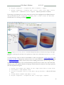
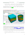
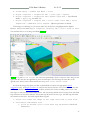
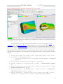
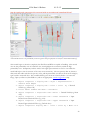
1
RVA Beta 0.1 Release 01-31-12 RVA: RESERVOIR VISUALIZATION AND ANALYSIS USER MANUAL Beta 0.1.0 D. Keefer, D. Torridi, J. Duggirala Copyright © 2011, University of Illinois at Urbana Champaign (UIUC). All Rights Reserved. 1 RVA Beta 0.1 Release 01-31-12 CONTENTS About .................................................................................................................................................................................... 4 Acknowledgements............................................................................................................................................................. 4 File Editing and Naming Convention for User Manual Authors ........................ Error! Bookmark not defined. Reservoir Visualization and Analysis Software .............................................................................................................. 5 Overview.......................................................................................................................................................................... 5 RVA Installation ............................................................................................................................................................. 5 Structure of the User Manual ....................................................................................................................................... 5 RVA and Reservoir Data ................................................................................................................................................... 6 RVA and Isatis Data ...................................................................................................................................................... 6 GTXserver Installation ............................................................................................................................................. 6 GTXserver Configuration ........................................................................................................................................ 6 Loading an Isatis Data Set ........................................................................................................................................ 8 Navigating Isatis File Structure................................................................................................................................ 9 RVA and UTCHEM Data .......................................................................................................................................... 10 RVA and Demonstration Data Sets .......................................................................................................................... 10 Font and Style Conventions Used in this Manual................................................................................................... 10 Getting to Know RVA..................................................................................................................................................... 12 The User Interface ....................................................................................................................................................... 12 Pipeline Browser ........................................................................................................................................................... 13 Visibility “Eye” Icon ............................................................................................................................................... 14 Renaming Objects ................................................................................................................................................... 14 Deleting Objects ...................................................................................................................................................... 14 Object Inspector........................................................................................................................................................... 14 Properties Tab .......................................................................................................................................................... 14 Display Tab ............................................................................................................................................................... 14 Information Tab ...................................................................................................................................................... 15 Filters 15 Recent Submenu ...................................................................................................................................................... 15 Common Submenu ................................................................................................................................................. 15 Data Analysis Submenu .......................................................................................................................................... 16 Alphabetical Submenu ............................................................................................................................................ 16 RVA Quickstart Tutorials................................................................................................................................................ 17 2 RVA Beta 0.1 Release 01-31-12 Basic ParaView-RVA Skills ......................................................................................................................................... 17 How do I change the vertical exaggeration for a data object?.......................................................................... 17 How do I add another viewing window to see a different view of my data?................................................. 17 How do I make a data object transparent? .......................................................................................................... 17 How do I show the axes for the data?.................................................................................................................. 17 I’ve added a second viewing window. How do I make the objects in each window spin together?.......... 18 How do I take a screenshot of my creation in ParaView? ................................................................................ 18 Exploring a geologic model............................................................................................................................................. 19 How do I use color shading to display different types of modeled data? ...................................................... 19 How do I use colored points to display my modeled data values? .................................................................. 21 How do I display my data using a wireframe format? ....................................................................................... 22 How do I display contours or isosurfaces in my data? ...................................................................................... 23 How do I display my data using a clip filter in RVA?........................................................................................ 24 How do I display my data set using the slice filter in RVA?............................................................. 26 How do I display my data set using a ................................................................................................................... 29 How do I display my data set using an IsoVolume filter in RVA? ................................................... 32 How do I display my data set using ...................................................................................................................... 33 How do I display my data in a spreadsheet for the filter that I applied in RVA? ................................ 36 How do I analyze modeled values in a spreadsheet when I used multiple filters? ............ 37 How do I model my borehole data using a glyph filter? ..................................................................... 39 How do I explore the sweet zone of my reservoir with my core data and normalized SP logs?................ 43 How do I save my progress so I will pick up where I left off at a later time? ............................................... 46 How do I load Saved State File?............................................................................................................................ 46 Exploring a Reservoir Fluid Simulation ........................................................................................................................ 46 3 RVA Beta 0.1 Release 01-31-12 ABOUT Reservoir Visualization and Analysis (RVA) was developed primarily through financial support from the U.S. Department of Energy – National Energy Technology Laboratory, under contract DE-FE0005961. Additional funding was provided by the State of Illinois, and the U.S. Geological Survey, under funding through the Great Lakes Geological Mapping Coalition, a program within National Cooperative Geologic Mapping Program. RVA is the result of a collaborative effort between the Illinois State Geological Survey at the Prairie Research Institute and the Department of Computer Science, both at the University of Illinois at Urbana-Champaign (UIUC). Project Geologists: D.Keefer and J.Damico. Software Development Team: L Angrave, E. Shaffer, D McWherter, U Yadav, and J Duggirala. Project Advisors: S. Frailey, R. Okwen, J. Grube, E. Mehnert, R. Ritzi, S. Whitaker, Y-F. Lin. Contact Us: [email protected] RVA is covered by Copyright (c) University of Illinois at Urbana-Champaign (UIUC). All rights reserved. This software is distributed WITHOUT ANY WARRANTY; without even the implied warranty of MERCHANTABILITY or FITNESS FOR A PARTICULAR PURPOSE. ACKNOWLEDGEMENTS RVA development was significantly benefitted by assistance from the following groups and individuals. Geovariances, France Center for Petroleum and Geosystems Engineering, University of Texas at Austin 4 RVA Beta 0.1 Release 01-31-12 RESERVOIR VISUALIZATION AND ANALYSIS SOFTWARE Overview RVA was developed to provide an integrated data visualization and analysis environment to support management of oil and gas reservoirs, particularly mature oil reservoirs being managed through tertiary recovery strategies known also as enhance oil recovery (EOR) strategies. The RVA software is a plugin to ParaView, an open-source 3-D visualization and analysis software package. The latest RVA build, source code, demonstration data sets and documentation are available free of charge from the project web site (http://rva.cs.illinois.edu). RVA is intended to open a range of data files frequently used by petroleum geologists and engineers involved with EOR projects, and to provide a suite of tools and tutorials for analyzing these varied data sets. Specific emphasis is placed on the development of novel tools for visualization and analysis of these complex data sets. Development of RVA has focused first on the creation of import utilities for bringing in geologic models and reservoir fluid simulation results. The first geologic model input format selected was for the geostatistical software, Isatis, a leading geostatistical analysis and simulation software package (Geovariances, France). In addition to Isatis, RVA is currently being expanded to import files from the reservoir simulation program, UTCHEM. This Beta 0.1 release contains a reader for several UTCHEM output files (.CONCP, .PRESP, .SATP, .VISC, .COMP-OIL, .COMP-ME, and .COMP-AQ). Development is continuing on the UTCHEM reader and additional file formats will be available soon. RVA functionality will build on the functionality inherent in ParaView. In addition, RVA will provide additional functionality that is not available through the standard ParaView builds. This RVA Users Manual will provide an overview of the ParaView concepts and tools that are critical for operating RVA. It will also provide instruction on the use of custom RVA tools and guidance on the use of RVA for common data visualization and analysis problems associated with EOR field management. Additional information on the use of ParaView can be obtained from the ParaView web page, or from the printed ParaView Users Manual (citation here). RVA Installation To install the current build of the RVA software, download and unzip the current build to your system. The current RVA build is for systems running Microsoft Windows operating system. Version-Specific: As of January, 2012, RVA has been tested and successfully operated on Windows Vista and Windows 7 operating systems. Please contact us if you have problems with installation. Structure of the User Manual This User Manual has been designed to help RVA users interact with their data as quickly as possible. Because RVA is a plugin to ParaView, there are many menus and buttons that are part of the standard ParaView interface and are available through RVA. However, this manual will only address key concepts in 5 RVA Beta 0.1 Release 01-31-12 ParaView and critical parts of the ParaView interface. Most of the manual will focus on using RVA-Paraview to open, visualize and analyze data associated with oil reservoir simulations. Rather than work through an exhaustive discussion of the menus, this manual has been structured in a question and answer format. This should allow the user to more quickly find solutions to problems or questions they want to address with RVA. This software and user manual are in active development and updates are expected frequently. Please note the software version and date stamps in the header of the User Manual. Compare your active version with the most recent versions available on the RVA project web site. The software is free and multiple versions can installed on a single computer. Please contact us if you have any feature requests, tutorial requests or bug reports. Users looking to expand their visualization and analytical capabilities within RVA are encouraged to explore the ParaView web site and to learn more about ParaView functionality. RVA AND RESERVOIR DATA RVA and Isatis Data Isatis project data are managed in a hierarchical directory structure where all of the data are stored as binary files. The Isatis developer, Geovariances, has provided a software development kit called GTXserver that allows programmers access to the native Isatis file structure. To enable RVA to read Isatis files, therefore, the GTXserver software needs to be installed and running. Procedures describing the installation and use of GTXserver are provided below. GTXserver Installation RVA utilizes the Geovariances GTXserver development kit to access and display data in existing Isatis study files. The Geovariances web site recommends working with GTXserver versions that are consistent with the Isatis version that created the files. Download the GTXserver zip file from http://www.geovariances.com/en/spip.php?page=GTXserver and extract it to your C drive. GTXserver Configuration Version Specific: The Beta 0.1 release is based on GTXserver 2011.2. If you have problems with version compatibility, we recommend you use the GTXserver version that is consistent with your Isatis file. If you continue to have difficulties either consult the Geovariances web page, or contact us for additional guidance. After downloading and extracting GTXserver, navigate to the folder C:\GTXserver\bin\winnt to find the GTXserver application. Create a shortcut for the application on your Desktop. Open the Properties dialog box by right clicking on the shortcut and selecting Properties. If you have saved GTXserver to your C drive then, in the Properties dialog box, set Target to: C:\GTXserver\bin\winnt\GTXserver.exe –multisession 6 RVA Beta 0.1 Release 01-31-12 If you have saved GTXserver elsewhere on your machine, set Target to the appropriate path. The option “–multisession” must follow the pathname of the GTXserver executable. When the target is properly specified, click to save and apply these changes. Fig: Change the Target field to C:\GTXserver\bin\winnt\GTXserver.exe –multisession, click OK. Launch GTXserver by double clicking the shortcut that you created, above. GTXserver is now running and RVA is ready to read your ISATIS files. Note: The GTXserver by default connects to port 5500. If you would like to change the port it uses, then use the “port” option in the Target field of the Properties dialog box ( –port XXXX). GTXserver MUST BE RUNNING on your system every time you want to access an Isatis file. 7 RVA Beta 0.1 Release 01-31-12 Loading an Isatis Data Set We provide example Isatis data for use in RVA. Download the Isatis demonstration case studies from the RVA website. Save the CaseStudies zip file and extract it to a convenient directory in your system. Open the Start Menu and type %APPDATA% in the search field. Click on the folder called Roaming. Then navigate to the folder called Geovariances followed by the folder Isatis. Within the Isatis folder you will be able to see a file called study_names.def (Fig 0.1). Fig 0.1: study_names file in the AppData\Roaming\Geovarianes\Isatis folder. Important: GTXserver and Isatis MUST NOT BE RUNNING when you open this file, or the changes you make will be overwritten Open study_names.def by right clicking on the file and selecting Open with and then Notepad. Modify the study_names.def file to add Demo_Data1 and Demo_Data2 as shown in Fig 0.2. Save and close study_names.def. Note: Users with an active Isatis license should find the study_names.def file already contains the names of studies loaded in their system previously. However it is possible that those studies may not be compatible with the GTXserver version you downloaded. To make sure your GTXserver installation and configuration were successful, add in the demonstration data set you downloaded from the RVA site. 8 RVA Beta 0.1 Release 01-31-12 Fig 0.2: Modified study_names file to include the RVA case studies –RVA_Demo1 and RVA_Demo2. Navigating Isatis File Structure Start RVA. Click on the RVA menu and select Import ISATIS Data. Version Specific: With the Beta 0.1 release, opening an Isatis study generates and error message. Please ignore this window. The Isatis import button creates an object called ISATISReader1 displayed in the Pipeline Browser. Next to the object cube you should see an icon that looks like an eye. The icon at this time will be grey in color indicating that no data can be seen in the view port as yet. The Properties tab in the Object Inspector panel shows seven fields all of which can be customized as per the choice of you. The GTX Server Port field will contain the port number that GTXserver is connected to. If GTXserver is running locally then type ‘localhost’ in the GTX Server Host field. The Refresh button must be clicked every time an RVA object is created in ParaView or when the port or the host is changed with the GTXserver connection. Clicking on the Refresh button establishes a connection between the machine that the server is running on and RVA so that the list of studies available on that machine become available to the local machine. If you are connected to a GTXserver running on the local machine then the studies available locally become available for reading into RVA. The text box next to the Refresh button will tell you the status of the connection every time it is clicked (Fig 0.2). The GTX Study field is a drop down list consisting of a list of studies that are populated by the connection to GTXserver. Selecting a valid study in this field will allow you to select a directory in the GTX Directory drop down list populated by the connection to GTXserver. Selecting a valid directory in this field will allow you to select a file in the GTX File Name field. It 9 RVA Beta 0.1 Release 01-31-12 contains the list of files available in the directory chosen above. Length Units can be used to view data scaled to the selected unit. Once all the fields are instantiated, click the Apply button to load the data. Note: Each time a new study/file/directory is chosen, the Apply button needs to be clicked. You have the additional option of Auto-Applying option in RVA. Navigate to Edit > Settings, check the Auto Accept box, click Apply and then OK. RVA and UTCHEM Data RVA is now able to read several UTCHEM output file types (.CONCP, .PRESP, .SATP, .VISC, .COMPOIL, .COMP-ME, and .COMP-AQ). Development on the UTCHEM reader is continuing and future releases of RVA will be able to read additional UTCHEM output file types. UTCHEM output files are in ascii format, allowing RVA to load these files directly through the Open command in the File Menu. RVA and Demonstration Data Sets Several demonstration project files are available for use with RVA. All the tutorials in this User Manual were made using two data files (Strat2fields.vts and BoreholeData.vtu). These files were created from an Isatis study, and saved in the ParaView-native vtk format. Strat2fields.vts contains a 3-D geostatistical model of porosity and permeability, while BoreholeData.vtu contains a 5-spot of wells with core porosity and permeability, and log data including SP and normalized SP. UTCHEM demo data are available from the RVA project web site. A zip file contains several different demonstration projects, each with several output files. All of these files can be opened through the File Menu, Open command. File Menu > Open = choose a demo file Objected Inspector > Property Tab > Apply Font and Style Conventions Used in this Manual This User Manual will use specific font and style notation to simplify instructions for completing specific tasks and when referring to parts of the RVA or ParaView interface. All instructions and interface names will use the Courier New font. Instructions for carrying out any procedure will use a carrot notation (>) to specify the flow of user interface choices. For example: Object Inspector > Display Tab > Color > Edit Color Map > Color Scale Tab > Choose Preset Button = Blue to Red Rainbow > OK > Close The above instructions specify how to select a preset color map (Blue to Red Rainbow) for an object. In this example, in the Object Inspector window, on the Display Tab, the Edit Color Map button was selected. In the pop up window for that button, the Choose Preset Button was selected. This 10 RVA Beta 0.1 Release 01-31-12 brought up another window on which the Blue to Red Rainbow preset color map was selected. The Ok and Close buttons were selected to finalize this choice. 11 RVA Beta 0.1 Release 01-31-12 GETTING TO KNOW RVA RVA is built on top of ParaView, an open source visualization and analysis package. The ParaView Home Page provides information on the background and structure of ParaView and links to a range of ParaView resources. There is an online users guide to ParaView, another online help for the current stable ParaView release, a tutorial for version 3.12, a group of more advance tutorials, newsgroups and user groups for general ParaView use. These resources do NOT cover RVA-specific tutorials or issues. This part of the User Manual discusses critical aspects of the generic, ParaView structure and functionality. These issues will be needed to make complete use of RVA. The User Interface The standard ParaView User Interface is shown in Figure 1. This figure highlights the modular nature and flexibility of the Paraview environment. Of particular note, the Pipeline Browser, Object Inspector, toolbars and varied view window types that are readily accessible. Figure 2 provides a view of the RVA User Interface. This figure shows the distinctive RVA menu and the banner text that contains the RVA @ UIUC reference and the build version. Figure 1. The ParaView User Interface. (from: http://paraview.org/Wiki/ParaView/Users_Guide/Introduction) 12 RVA Beta 0.1 Release 01-31-12 Figure 2. RVA User Interface. Note the RVA menu, and the RVA@UIUC with build version in the banner. In ParaView, there will always be one “active” view, one “active” module or object within the visualization pipeline, and one “active” selection. The information displayed in any region of the User Interface always relates to these active entities (ParaView Users Guide). Within ParaView, there are three basic steps to visualizing data: reading the data into ParaView, filtering or processing the data in some way, and rendering or drawing some aspect of the data. RVA, as a plugin to ParaView, is focused on simplifying the processes of reading data into ParaView and of filtering the data, all with the goal of simplifying visualization and analysis of reservoir simulation results and thereby improving the management of mature oil fields. ParaView takes these three steps and integrates them with an architecture called the visualization pipeline, which allows a user to read in data and run the data through a sequence of processes, or filters, each of which provide a different view of the data. ParaView has over one hundred different filters that can be used to manipulate various data types. Since the filters are specific to the type of data processed, not all filters work on all data sets. When a filter is unavailable for an active data object, it is greyed out in the menu. Pipeline Browser The Pipeline Browser is where the visualization pipeline is recorded and controlled from (ParaView Users Guide). As such interaction with the Pipeline Browser is a critical component of RVA. The following describes some of the more important aspects of the Pipeline Browser. 13 RVA Beta 0.1 Release 01-31-12 Visibility “Eye” Icon On loading data the visibility, or eye, icon next to the object in the Pipeline Browser turns from grey to black. This indicates whether or not an object is rendered in the active window. Clicking on the eye icon changes the icon from black to grey and correspondingly toggles the object from rendered to not rendered. This eye icon is useful when multiple objects are available for viewing. The behavior of the Eye Icon can vary when multiple display windows are used. Use of multiple display windows will be covered later in the manual. Renaming Objects Objects created can be renamed in the Pipeline Browser. The objects by default are named alphanumerically with the name of the object followed by the creation number. Double clicking on this name opens a text edit box where you can rename the object to be more informative. Deleting Objects You can right click on an object for a list of actions to take on the object. Clicking on Delete will remove the object from the Pipeline Browser. Object Inspector The Object Inspector is where the various parameters of the active module within the visualization pipeline are displayed and controlled from. Properties Tab The Properties Tab of the Object Inspector holds information on the filters and objects created in the Pipeline Browser. All of the fields in the Properties Tab change the configuration of the objects. The Apply button must be clicked each time there is change made to an object in the Properties Tab. ParaView has the additional option of auto-applying changes made to the Properties Tab. To autoapply changes to the Properties Tab: Edit Menu > Settings > General Settings >Auto Accept = check/uncheck > OK Display Tab In the Display Tab the following are useful functions for viewing data objects for better: Zoom To Data – This button centers all of the data objects that are turned on in the active viewing window. Color by – This field applies color to the data set according to the variable selected. In the drop down a list of variables appear and you can then use any one of the variables to color the data set. To see the list of variables corresponding to a given data object the Representation field (details given below) needs to be set to anything except Outline. Edit Color Map… - This button opens a widget to adjust the color scales on the data. The Choose Preset button in the Color Scale tab shows a list of color schemes available with the data. The checkbox for Use Logarithmic Scale sets colors using a log scale. The Color Legend tab displays the legend for the current variable being used on the view port. 14 RVA Beta 0.1 Release 01-31-12 Set Ambient Color… - This drop down list can be used to set solid color to the data using the colors provided by ParaView. Show cube axes – When checked, this box displays the appropriately labeled axes for the selected object. The Edit button allows for customization of the drawing options for each of the axes. Representation – This drop down list consists of different ways to draw an object. To see the variables for the object you must set the Representation to anything except Outline. The list of variables can be viewed through the dropdown list in Color > Color by. Point Size/Line Width/Opacity – Increasing or decreasing these values changes the appearance of the data accordingly. Translate/Scale/Orientation/Origin – These fields in the Display tab transform the data based on the given input. The data only changes when the values are typed into the boxes and then clicking the mouse away from the boxes (i.e. losing focus from the boxes). In most cases this operation needs to be followed by clicking on Zoom To Data to center the data correctly. Unlike the Properties tab there is no need to click the Apply button when fields are changed in the Display tab. Pressing the TAB button or selecting another field in the Display Tab applies the changes that have been made. Most of the above operations can also be done using the icons in the Representation and Active Variable Controls toolbars from the ParaView main window. Information Tab The Information Tab in the Object Inspector provides information on the data objects including the Type, Number of Cells, Number of Points, the Data Arrays/Variable List, the Extents and the Bounds. The fields indicate the data structure used to represent the data, the volume of interest and the number of samples present in the given data set. Filters As mentioned above, ParaView has over one hundred filters for processing the information associated with active objects in the visualization pipeline. These filters are accessed through the Filters Menu on the MenuBar. The filters are displayed under four submenus: Recent, Common, Data Analysis and Alphabetical. Recent Submenu The Recent submenu lists the 10 most recent filters used. Common Submenu Common displays the filters that most ParaView users will use most commonly. You can find shortcuts to these filters on the Filters Toolbar. Some of the common filters used are: Glyphs - This filter produces glyphs at each point in the selected data set. Different shapes can be used for the glyphs like cone, arrow, line, sphere or 2D glyph. Threshold – This filter extracts the subset of the data set whose scalars lie within the specified range. The Lower Threshold and Upper Threshold sliders indicate the range of scalars to retain in the data set. 15 RVA Beta 0.1 Release 01-31-12 Contour – This filter calculates the Isolines/Isosurfaces of the selected point centered scalar array in the data set. The available scalars are listed in the Contour by dropdown list. To add a single contour value, select the New Value field in the Isosurfaces section of the Properties tab and type a new value. To add several evenly spaced values first click on Delete All button which deletes the initial values present, then click New Range and type in the values in the From, To and Steps text boxes to specify the Contour values and the spacing interested. If you would like to space the contours using a Logarithmic scale instead of a liner scale then check the Use Logarithmic Scale option in the dialog box and press OK to add the values or Cancel to not add them. The Contour filter operates on any data set that has atleast one point-centered scalar array. The output is a polygonal mesh. You can also check the Compute Normals, Compute Gradients, Compute Scalars and the corresponding computation is performed and the contours are Displayed accordingly. Slice – This filter extracts the portion of the data set along a plane. The plane can be specified by using the interactive widget/axes or by manually typing in the values in the Transformation box. Using the Slice Offset Values you can also slice a portion of the data set using an offset from the original plane function. The Offset Values can be added in a similar fashion by adding New Value/New Range in the dialog box. Clip – This filter clips away a portion of the data set depending on the Clip Type selected in the Properties tab of the Object Inspector. You has the choice of selecting a plane, box, sphere or scalar. The Clip filter returns the portion of the data set that remains after the clip. If the scalars option is chosen then you must select the scalar array by which to clip. Clip then returns the set of those scalars that are larger than the clip Value. Checking the Inside Out box will return the portion that has been clipped rather than the portion that remains after the clip. Data Analysis Submenu These filters can be used to analyze data quantitatively. They can plot data as graphs and histograms on different variables. Alphabetical Submenu This option lists all the available filters in an alphabetical order. The screenshots given at the end of this manual illustrate the use of some of these filters. For more details on how to use ParaView please see Additional References at the end of this manual. 16 RVA Beta 0.1 Release 01-31-12 RVA QUICKSTART TUTORIALS Basic ParaView-RVA Skills How do I change the vertical exaggeration for a data object? The vertical exaggeration is adjusted from the Display Tab. To set the vertical exaggeration for an object to 10x: Display Tab > Transformation > Scale = 1, 1, 10 This only works on one object at a time. It generally does carry forward to new daughter objects. If you set the vertical exaggeration for a geologic model to 10, then use a Threshold Filter on this model, the Threshold Filter object is automatically set to 10. However, if you subsequently change the original geologic model to 5, the Threshold Filter object is not updated automatically. Also, some filters do not inherit these scaling changes. For example, the Clip and Slice filters load with the default scale values, regardless of vertical, or horizontal, change in scale of the parent filter or data object. How do I add another viewing window to see a different view of my data? Each viewing window can be subdivided into multiple viewing windows, with each new window set to be a different window type (e.g., 3D View, 2D View, Spreadsheet View). Any active viewing window can be split horizontally or vertically. The split window buttons are located in the upper right hand corner of each view window (Fig 1.4). Once the window is split, a list of window types is provided. Choose the desired window type. The active viewing window is identified by a blue border. The data objects that have been included in the active window are identified by black eye icons. To add a data layer to the active window, select the desired window, then select the desired object(s) from the Pipeline Browser. Fig 1.4: Split Horizontal, Split Vertical, Maximize, Close. How do I make a data object transparent? To change the opacity of an object, you adjust the Opacity field between 0 and 1, with 1 being completely opaque and 0 being completely transparent. Object Inspector > Display Tab > Style > Opacity = choose a value (e.g., 0.5) How do I show the axes for the data? The axes are readily drawn for any data layer . Object Inspector > Display Tab > Annotation > Show Cube Axes = checked/unchecked. The details of each axis can also be adjusted. Object Inspector > Display Tab > Annotation > Edit (each axis can be adjusted as desired) 17 RVA Beta 0.1 Release 01-31-12 . I’ve added a second viewing window. How do I make the objects in each window spin together? ParaView has the useful option of linking two images in different view ports so that they can both be oriented in the same position at the same time. When one image is rotated in one direction the other image with the camera link rotates in that direction too. Tools Menu > Add Camera Link This opens up a dialog box like the one in Fig 4.3. Click on the window that you want to link with the window that has the dialog box. When you click on the other window a link is established. Clicking on Zoom To Data might be necessary to focus both the objects correctly. Now rotating one object in a certain direction also rotates the other object in that direction. Fig 4.3: A dialog box opens when you Add Camera Link. Now click on the window marked in red to establish a camera link between the two windows. How do I take a screenshot of my creation in ParaView? Navigate to File Menu in the menu bar and select Save Screenshot. This opens a dialog box with the options to configure the output image file. Click on OK after you make the changes of your choice, save the picture and you have a copy of your creation. 18 RVA Beta 0.1 Release 01-31-12 EXPLORING A GEOLOGIC MODEL How do I use color shading to display different types of modeled data? Figure 5.1 A surface representation was used on the permeability values to create the above image . To shade a volume model by the variations in a variable, Open your data set (Strat2fields.vts) and set the appropriate vertical exaggeration (10x). The first step will select surface representation for the data rendering. The second step will choose a variable, the values of which will be used to color the data set. The third step will be to set the color mapping. The fourth step will draw the legend. 1. Object Inspector > Display Tab > Style > Representation = Surface 2. Object Inspector > Display Tab > Color > Color by = choose a variable (e.g., Mean of K) 3. Object Inspector > Display Tab > Color > Edit Color Map > Choose Preset = RVA_Rainbow1 4. Object Inspector > Display Tab > Color > Edit Color Map > Color Legend Tab > check Show Color Legend. Adjust the parameters as desired. If this image is not drawing on your screen, make sure the Eye Icon is highlighted in the Pipeline Browser. Also you can check Object Inspector > Display Tab > View > Zoom to Data. You should be able to see an image resembling Figure 5.1. 19 RVA Beta 0.1 Release 01-31-12 Figure 5.2 A surface with edges representation was used on the permeability values to create the above image. A similar view is the surface with edges representation. This provides a way to view the cell boundaries as well as the modeled variable values. To make this image, Open your data set (Strat2fields.vts) and set the appropriate vertical exaggeration (10x). The first step will render the data using a surface with edges representation. The second step will choose a variable, the values of which will be used to color the data set. The third step will be to set the color mapping. The fourth step will draw the legend. 1. Object Inspector > Display Tab > Style > Representation = Surface with Edges 2. Object Inspector > Display Tab > Color > Color by = choose a variable (e.g., Mean of K ) 3. Object Inspector > Display Tab > Color > Edit Color Map > Choose Preset = RVA_Rainbow1 4. Object Inspector > Display Tab > Color > Edit Color Map > Color Legend Tab > check Show Color Legend. Adjust the parameters as desired. If this image is not drawing on your screen, make sure the Eye Icon is highlighted in the Pipeline Browser. Also you can check Object Inspector >Display Tab > View > Zoom to Data. You should be able to see an image resembling Figure 5.2. 20 RVA Beta 0.1 Release 01-31-12 How do I use colored points to display my modeled data values? Figure 5.3 A points representation was used on the permeability values to create the above image . Another valuable visualization tool is to draw the cell nodes and color them by a modeled variable. To create this image, Open your data set (Strat2fields.vts) and set the appropriate vertical exaggeration (10x). The first step will select the point representation for the data. The second step will be to adjust the size of the points. The third step will choose a variable, the values of which will be used to color the data set. The fourth step will be to set the color mapping. The fifth step will draw the legend. 1. Object Inspector > Display Tab > Style > Representation = Points 2. Object Inspector > Display Tab > Style > Point Size= choose a size (e.g., 5.00) 3. Object Inspector > Display Tab > Color > Color by = choose a variable (e.g., Mean of K ) 4. Object Inspector > Display Tab > Color > Edit Color Map > Choose Preset = RVA_Rainbow1 5. Object Inspector > Display Tab > Color > Edit Color Map > Color Legend Tab > check Show Color Legend. Adjust the parameters as desired. If this image is not drawing on your screen, make sure the Eye Icon is highlighted in the Pipeline Browser. Also you can check Object Inspector >Display Tab > View > Zoom to Data. You should be able to see an image resembling Figure 5.3. 21 RVA Beta 0.1 Release 01-31-12 How do I display my data using a wireframe format? Figure 5.4 A wireframe representation was used on the permeability values to create the above image. To create this image, first Open your data set (Strat2fields.vts) and set the appropriate vertical exaggeration (10x). The first step will show the data using a wireframe representation. The second step will choose a variable, the values of which will be used to color the data set. The third step will be to set the color mapping. The fourth step will draw the legend. 1. Object Inspector > Display Tab > Style > Representation = Wireframe 2. Object Inspector > Display Tab > Color > Color by = choose a variable (e.g., Mean of K ) 3. Object Inspector > Display Tab > Color > Edit Color Map > Choose Preset = RVA_Rainbow1 4. Object Inspector > Display Tab > Color > Edit Color Map > Color Legend Tab > check Show Color Legend. Adjust the parameters as desired. If this image is not drawing on your screen, make sure the Eye Icon is highlighted in the Pipeline Browser. Also you can check Object Inspector >Display Tab > View > Zoom to Data. You should be able to see an image resembling Figure 5.4. 22 RVA Beta 0.1 Release 01-31-12 How do I display contours or isosurfaces in my data? Figure 5.5 A contour filter was used on the permeability values to create the above image. The contours that are displayed are between the range of 100- 200 with a contour interval of 10. The Contour Filter can be used to create a single isosurface, or a set of isosurfaces for a geologic model or reservoir simulation. To create this image, first Open your data set (Strat2fields.vts) and set the appropriate vertical exaggeration (10x). The first step will apply a contour filter to the data set. The second and third steps will select the variable used in contouring. The fourth step will remove the default contour values. The fifth and sixth steps will set the range of contour values. The seventh step will set the variable to use for coloring the isosurfaces. The sixth step will draw the legend. 1. Filter Menu > Common Submenu = Contour 2. Object Inspector > Properties Tab> Contour >Contour by= choose a viable (e.g., Mean of K ) 3. Object Inspector > Properties Tab > Contour > check Compute Scalars 4. Object Inspector > Properties Tab > Isosurfaces = Delete All ( to remove the default value) 5. Object Inspector > Properties > Isosurfaces > New Range 6. Add Range Pop Up Window > Input Desired Range and Desired Steps > Apply (e.g., 100-250 range with 4 steps ) 7. Object Inspector > Display Tab >Color > Color by= choose a variable (e.g., Mean of K) 8. Object Inspector > Display Tab > Color > Edit Color Map > Color Legend Tab > check Show Color Legend. Adjust the parameters as desired. 23 RVA Beta 0.1 Release 01-31-12 If this image is not drawing on your screen, make sure the Eye Icon is highlighted in the Pipeline Browser. Also you can check Object Inspector >Display Tab > View > Zoom to Data. You should be able to see an image resembling Figure 5.5. How do I display my data using a clip filter in RVA? Figure 5.6 A plane clip filter was used on the permeability values to create the above image on the right hand side. For this image the same data set was opened in two camera views to demonstrate how the clip filter works. A clip filter cuts and removes portions of an object, allowing the remaining, uncut portions to be rendered. ParaView provides a few distinct clipping shapes to apply to data: a plane, a box, a sphere and a scalar value (of the variable used in the coloring of the object). The clip can also be “reversed” by checking the Inside Out check box on the Properties Tab. To create this image, first Open your data set (Strat2fields.vts) and set the appropriate vertical exaggeration (10x). To display your data set, reference the section on how to use a color shade on your data in RVA. To display two linked camera views in RVA, reference this section on adding camera views. The first step is to make sure the correct image chosen. The second and third steps link the two camera views. The fourth step sets the clip filter and the fifth step selects the type of clip that is used. The sixth step set the the plane to be clipped along. The seventh step draws the legend. 1. Select with mouse the image on the right hand side to work with. 2. Tools Menu> Add Camera Link 3. Click on Another View to Link With Pop Up Window > click the left Camera View 4. Filter Menu> Common Sub Menu = Clip 5. Object Inspector > Properties Tab> Clip Type = Plane 24 RVA Beta 0.1 Release 01-31-12 6. Object Inspector > Properties Tab> X Normal > Apply 7. Object Inspector > Display Tab > Color > Edit Color Map > Color Legend Tab > check Show Color Legend. Adjust the parameters as desired. If this image is not drawing on your screen, make sure the Eye Icon is highlighted in the Pipeline Browser. Also you can check Object Inspector >Display Tab > View > Zoom to Data. You should be able to see an image resembling Figure 5.6. Figure 5.8 A spherical clip filter was used on the porosity values to create the above image on the right hand side. For this image the same data set was opened in two camera view to demonstrate how the clip filter works. To create this image, Open your data set (Strat2fields.vts) and set the appropriate vertical exaggeration (10x). To display your data set, reference the section on how to use a color shade on your data in RVA. To display two linked camera views in RVA, reference this section on adding camera views. The first step is to make sure the correct image chosen. The second and third step will link the two camera views. The fourth, fifth and sixth steps set the clip filter function, the clip type, and the Inside Out character of the clip, respectively. The sixth step draws the legend. 1. Select with mouse the image on the right hand side to work with. 2. Tools Menu > Add Camera Link 3. Click on Another View to Link With Pop Up Window > click the left Camera View 4. Filter Menu> Common Sub Menu = Clip 5. Object Inspector > Properties Tab > Clip Type = Sphere 25 RVA Beta 0.1 Release 01-31-12 6. Object Inspector > Properties Tab > Inside Out check the box > Apply 7. Object Inspector > Display Tab > Color > Edit Color Map > Color Legend Tab > check Show Color Legend. Adjust the parameters as desired. If this image is not drawing on your screen, make sure the Eye Icon is highlighted in the Pipeline Browser. Also you can check Object Inspector >Display Tab > View > Zoom to Data. You should be able to see an image resembling Figure 5.8. How do I display my data set using the slice filter in RVA? Figure 5.9 A sphere slice filter was used on the permeability values to create the above image on the right hand side. For this image the same data set was opened in two camera views to demonstrate how the sphere slice filter works. A slice filter shows the values of an object ONLY where it intersects with a 2-D plane or surface. This can create simple cross section views, to more elaborate images like in figure 5.9. To create this image, Open your data set (Strat2fields.vts) and set the appropriate vertical exaggeration (10x). To display your data set, read the section on how to color your data in RVA. To display two linked camera views in RVA, read this section on adding camera views. The first step in making this image selects the correct image. The second step will link the two camera views. The third step will choose the slice filter function. The fourth step will choose the slice type. .The fifth step will change the radius of the slice. The sixth step will draw a legend. 1. Select with mouse the image on the right hand side to work with. 2. Tools Menu > Add Camera Link 3. Click on Another View to Link With Pop Up Window > click the left Camera View 26 RVA Beta 0.1 Release 01-31-12 4. Filter Menu] > Common Sub Menu = Slice 5. Object Inspector > Properties Tab > Slice Type = Sphere 6. Object Inspector > Properties Tab> Radius Input Box = Input Desired Radius -> Apply (e.g., the radius 375) 7. Object Inspector > Display Tab > Color > Edit Color Map > Color Legend Tab > check Show Color Legend. Adjust the parameters as desired. If this image is not drawing on your screen, make sure the Eye Icon is highlighted in the Pipeline Browser. Also you can check Object Inspector >Display Tab > View > Zoom to Data. You should be able to see an image resembling Figure 5.9. Figure 5.10 A plane slice filter was used on the permeability values to create the above image on the right hand side. The slice was applied along the Z Normal option. For this image the same data set was opened in two camera views to demonstrate how the plane slice filter works. To create this image, first Open your data set (Strat2fields.vts) and set the appropriate vertical exaggeration (10x). To display your data set, reference the section on how to use a color shade on your data in RVA. To display two linked camera views in RVA, reference this section on adding camera views. The first step is to make sure the correct image chosen. The second step will link the two camera views. The third step will choose the slice filter function. The fourth step will choose the slice type. The fifth step will select the orientation of the slice. The sixth step will draw a legend. 1. Select with mouse the image on the right hand side to work with. 2. Tools Menu> Add Camera Link a. Click on Another View to Link With Pop Up Window> click the left Camera View 27 RVA Beta 0.1 Release 3. 4. 5. 6. Filter Object Object Object Legend 01-31-12 Menu > Common Sub Menu = Slice Inspector > Properties Tab > Slice Type = Plane Inspector > Properties Tab > Select Z Normal Button Inspector > Display Tab > Color > Edit Color Map > Color Tab > check Show Color Legend. Adjust the parameters as desired. If this image is not drawing on your screen, make sure the Eye Icon is highlighted in the Pipeline Browser. Also you can check Object Inspector >Display Tab > View > Zoom to Data. You should be able to see an image resembling Figure 5.10. Figure 5.12 A plane slice filter was used on the permeability values to create the above image on the right hand side. The slices for this example were along the Y Normal option with multiple slices. For this image the same data set was opened in two camera views to demonstrate how the slice filter works. To create this image, first Open your data set (Strat2fields.vts) and set the appropriate vertical exaggeration (10x). To display your data set, reference the section on how to use a color shade on your data in RVA. To display two linked camera views in RVA, reference this section on adding camera views. The first step is to make sure the correct image chosen. The second step will link the two camera views. The third step will choose the slice filter function. The fourth step will choose the slice type. The fifth step will select the orientation of the slice. The sixth will select the slice offset values range. The seventh step will draw a legend. 1. Select with mouse the image on the right hand side to work with. 28 RVA Beta 0.1 Release 01-31-12 2. Tools Menu > Add Camera Link a. Click on Another View to Link With Pop Up Window > click the left Camera View 3. Filter Menu > Common Sub Menu = Slice 4. Object Inspector > Properties Tab > Slice = Plane 5. Object Inspector > Properties Tab > Select Y Normal Button 6. Object Inspector > Properties Tab > Slice Offset Values > New Range Button a. Add Range Pop Up Window > Input Desired Range and Desired Steps > Apply (e.g., used the default values ) 7. Object Inspector > Display Tab > Color > Edit Color Map > Color Legend Tab > check Show Color Legend. Adjust the parameters as desired. If this image is not drawing on your screen, make sure the Eye Icon is highlighted in the Pipeline Browser. Also you can check Object Inspector >Display Tab > View > Zoom to Data. You should be able to see an image resembling Figure 5.11. How do I display my data set using a threshold filter in RVA? Figure 5.12 A threshold filter was used on the porosity values to create the above image on the right hand side. For this image the same data set was opened in two camera views to demonstrate how the threshold filter works. The threshold filter function allows the user to look at different ranges of values within their data set. This allows the user to focus in on specific areas of interest. 29 RVA Beta 0.1 Release 01-31-12 To create this image, first Open your data set (Strat2fields.vts) and set the appropriate vertical exaggeration (10x). To display your data set, reference the section on how to use a color shade on your data in RVA. To display two linked camera views in RVA, reference this section on adding camera views. The first step is to make sure the correct image chosen. The second step will link the two camera views. The third step will choose the threshold filter function. The fourth step will select the scalar variable. The fifth step will select lower threshold value. The sixth will select the upper threshold value. The seventh step will draw a legend. 1. Select with mouse the image on the right hand side to work with. 2. Tools Menu> Add Camera Link a. Click on Another View to Link With Pop Up Window > click the left Camera View 3. Filter Menu > Common Sub Menu = Threshold 4. Object Inspector > Properties Tab > Scalar = Desired Variable (e.g. Mean of Phi) 5. Object Inspector > Properties Tab > Lower Threshold > Input Desired Lower Threshold Value (e.g., 16) 6. Object Inspector > Properties Tab > Upper Threshold > Input Desired Upper Threshold Value > Apply (e.g., 21) 7. Object Inspector > Display Tab > Color > Edit Color Map > Color Legend Tab > check Show Color Legend. Adjust the parameters as desired. If this image is not drawing on your screen, make sure the Eye Icon is highlighted in the Pipeline Browser. Also you can check Object Inspector >Display Tab > View > Zoom to Data. You should be able to see an image resembling Figure 5.12. 30 RVA Beta 0.1 Release 01-31-12 Figure 5.13 The above image on the right hand side was created using a threshold filter. The data set was colored with the permeability values; the filter was applied to the porosity values in the data set. For this image the same data set was opened in two camera views to demonstrate how the threshold filter works. To create this image, first Open your data set (Strat2fields.vts) and set the appropriate vertical exaggeration (10x). To display your data set, reference the section on how to use a color shade on your data in RVA. To display two linked camera views in RVA, reference this section on adding camera views. The first step is to make sure the correct image chosen. The second step will link the two camera views. The third step will choose the threshold filter function. The fourth step will select the scalar variable. The fifth step will select lower threshold value. The sixth will select the upper threshold value. The seventh step will draw a legend. 1. Select with mouse the image on the right hand side to work with. 2. Tools Menu > Add Camera Link a. Click on Another View to Link With Pop Up Window > click the left Camera View 3. Filter Menu> Common Sub Menu = Threshold 4. Object Inspector> Properties Tab > Scalar= Desired Variable(e.g., Mean of Phi) 5. Object Inspector > Properties Tab > Lower Threshold > Input Desired Lower Threshold Value (e.g., 16.) 6. Object Inspector > Properties Tab > Upper Threshold > Input Desired Upper Threshold Value (e.g., 20.) 7. Object Inspector > Display Tab > Color > Edit Color Map > Color Legend Tab > check Show Color Legend. Adjust the parameters as desired. If this image is not drawing on your screen, make sure the Eye Icon is highlighted in the Pipeline Browser. Also you can check Object Inspector >Display Tab > View > Zoom to Data. You should be able to see an image resembling Figure 5.13. 31 RVA Beta 0.1 Release 01-31-12 How do I display my data set using an IsoVolume filter in RVA? Figure 5.15 A IsoVolume filter was used on the permeability values to create the above image on the right hand side. For this image the same data set was opened in two camera views to demonstrate how the IsoVolume filter works. To create this image, first Open your data set (Strat2fields.vts) and set the appropriate vertical exaggeration (10x). To display your data set, reference the section on how to use a color shade on your data in RVA. To display two linked camera views in RVA, reference this section on adding camera views. The first step is to make sure the correct image chosen. The second step will link the two camera views. The third step will choose the isovolume filter function. The fourth step will select the scalar variable. The fifth step will select lower threshold value. The sixth will select the upper threshold value. The seventh step will draw a legend. 1. Select with mouse the image on the right hand side to work with. 2. Tools Menu > Add Camera Link > a. Click on Another View to Link With Pop Up Window > click the left Camera View 3. Filter Menu > Alphabetical Sub Menu = IsoVolume 4. Object Inspector > Properties Tab > Scalar = Desired Variable (e.g., Mean of K) 5. Object Inspector > Properties Tab > Lower Threshold Option = Input Desired Lower Threshold Value (e.g., 65) 6. Object Inspector > Properties Tab] > Upper Threshold = Input Desired Upper Threshold Value> Apply (e.g., 190). 7. Object Inspector > Display Tab > Color > Edit Color Map > Color Legend Tab > check Show Color Legend. Adjust the parameters as desired. 32 RVA Beta 0.1 Release 01-31-12 If this image is not drawing on your screen, make sure the Eye Icon is highlighted in the Pipeline Browser. Also you can check Object Inspector >Display Tab > View > Zoom to Data. You should be able to see an image resembling Figure 5.14. How do I display my data set using multiple filters in RVA? Figure 5.15 A sphere clip filter and a contour filter was used on the permeability values to create the above image on the right hand side. For this image the same data set was opened in two camera view to demonstrate how the clip filter works To create this image, first Open your data set (Strat2fields.vts) and set the appropriate vertical exaggeration (10x). To display your data set, reference the section on how to use a color shade on your data in RVA. To display two linked camera views in RVA, reference this section on adding camera views. The first step is to make sure the correct image chosen. The second step will link the two camera views. The third step will choose the clip filter function. The fourth step will select the clip type. The fifth step will add the contour filter function. The sixth step will select the variable to contour by. The seventh step will remove default range values. The eight step will select a new range of values to contour by. The ninth step will draw a legend. 1. Select with mouse the image on the right hand side to work with. 2. Tools Menu > Add Camera Link a. Click on Another View to Link With Pop Up Window > click the left Camera View 3. Filter Menu > Common Sub Menu = Clip 4. Object Inspector > Properties Tab > Clip Type = Sphere 33 RVA Beta 0.1 Release 01-31-12 Object Inspector > Properties Tab > Inside Out check the box > Apply Filter Menu > Common Sub Menu > Contour (Note that the right hand image still needs to be selected) Object Inspector > Properties Tab > Contour > Contour By = Desired Variable (e.g., Mean of K ) Object Inspector -> Properties Tab > Isosurfaces = Delete All ( to remove the default value) Object Inspector > Properties Tab > Isosurfaces > New Range a. Add Range Pop Up Window > Input Desired Range and Desired Steps > Apply (e.g., used the default values ) Object Inspector > Display Tab > Color > Edit Color Map > Color Legend Tab > check Show Color Legend. Adjust the parameters as desired. a. 5. 6. 7. 8. 9. If this image is not drawing on your screen, make sure the Eye Icon is highlighted in the Pipeline Browser. Also you can check Object Inspector >Display Tab > View > Zoom to Data. You should be able to see an image resembling Figure 5.15. Figure 5.16 A sphere clip filter and a threshold filter was used on the porosity values to create the above image on the right hand side. For this image the same data set was opened in two camera view to demonstrate how the clip filter and threshold filter work To create this image, first Open your data set (Strat2fields.vts) and set the appropriate vertical exaggeration (10x). To display your data set, reference the section on how to use a color shade on your data in RVA. To display two linked camera views in RVA, reference this section on adding camera views. The first step is to make sure the correct image chosen. The second step will link the two camera views. The third 34 RVA Beta 0.1 Release 01-31-12 step will choose the clip filter function. The fourth step will select the clip type. The fifth step will add the threshold filter function. The sixth step will select the scalar variable. The seventh step will select the lower threshold value. The eighth step will select the upper threshold value. The ninth step will draw a legend. 1. Select with mouse the image on the right hand side to work with. 2. Tools Menu > Add Camera Link a. Click on Another View to Link With Pop Up Window > click the left Camera View 3. Filter Menu> Common Sub Menu = Clip 4. Object Inspector > Properties Tab > Clip Type = Sphere a. Object Inspector > Properties Tab = check Inside Out > Apply 5. Filter Menu> Common Sub Menu = Threshold (Note that the right hand image still needs to be selected) 6. Object Inspector > Properties Tab > Scalar= Desired Variable(e.g., Mean of Phi) 7. Object Inspector > Properties Tab > Lower Threshold = Input Desired Lower Threshold Value (e.g., 16) 8. Object Inspector > Properties Tab> Upper Threshold = Input Desired Upper Threshold Value > Apply (e.g., 21) 9. Object Inspector > Display Tab > Color > Edit Color Map > Color Legend Tab > check Show Color Legend. Adjust the parameters as desired. If this image is not drawing on your screen, make sure the Eye Icon is highlighted in the Pipeline Browser. Also you can check Object Inspector >Display Tab > View > Zoom to Data. You should be able to see an image resembling Figure 5.16. 35 RVA Beta 0.1 Release 01-31-12 How do I display my data in a spreadsheet for the filter that I applied in RVA? Figure 5.17 A threshold filter was used on the porosity values to create the above image on the left hand side. The results of the threshold filter are displayed in the spreadsheet on the right hand side. To create this image, first Open your data set (Strat2fields.vts) and set the appropriate vertical exaggeration (10x). To display your data set, reference the section on how to use a color shade on your data in RVA. The first step will add the threshold filter function to your data set. The second step will select the scalar variable. The third step will select the lower threshold value. The fourth step will select the upper threshold value. The fifth step will draw a legend. The sixth step will split the camera view and add a spreadsheet. The seventh will show the results of the desired filter. 1. Filter Menu > Common Sub Menu = Threshold 2. Object Inspector > Properties Tab> Scalar = Desired Variable(e.g. Mean of K) 3. Object Inspector > Properties Tab > Lower Threshold = Input Desired Lower Threshold Value (e.g. 218) 4. Object Inspector > Properties Tab > Upper Threshold = Input Desired Upper Threshold Value (e.g., 250). a. Object Inspector > Properties Tab > Uncheck All Scalars > Apply 5. Object Inspector > Display Tab > Color > Edit Color Map > Color Legend Tab > check Show Color Legend. Adjust the parameters as desired. 6. View Port > Slit Horizontal >Spreadsheet View 7. Spreadsheet > Showing = Threshold1 36 RVA Beta 0.1 Release 01-31-12 Now you are able to use the spreadsheet to analyze the results of the threshold filter. If this image is not drawing on your screen, make sure the Eye Icon is highlighted in the Pipeline Browser. Also you can check Object Inspector >Display Tab > View > Zoom to Data. You should be able to see an image resembling Figure 5.17. How do I analyze modeled values in a spreadsheet when I used multiple filters? Figure 5.18 .A slice filter was used on the permeability values to create the above image on the left hand side. The image on the right was created by adding a threshold filter to the sliced filter on the right hand side. The results of the threshold filter are displayed in the spreadsheet along the bottom of the display. To create this image, first Open your data set (Strat2fields.vts) and set the appropriate vertical exaggeration (10x). To display your data set, reference the section on how to use a color shade on your data in RVA. To display two linked camera views in RVA, reference this section on adding camera views. The first step is to make sure the correct image chosen. The second step will link the two camera views. The third step will choose the slice filter function. The fourth step will select the slice type. The fifth step will remove default slice offset value. The sixth step will add a new range of slice offset values. The seventh step will repeat steps 3 through 6a with the right hand camera view. The eighth step will add a threshold filter to the right hand camera view. The ninth step will select the scalar variable. The tenth step will select the lower threshold value. The eleventh step will select the upper threshold value. The twelfth step will draw a legend. The thirteenth step will split the camera view and add a spreadsheet. The fourteenth will show the results of the desired filter in spreadsheet view. 1. Select with mouse the image on the left hand side to work with. 37 RVA Beta 0.1 Release 2. 3. 4. 5. 6. 7. 8. 9. 10. 11. 12. 13. 14. 01-31-12 Tools Menu > Add Camera Link a. Click on Another View to Link With Pop Up Window > click the left Camera View Filter Menu> Common Sub Menu = Slice (left hand camera view selected) Object Inspector > Properties Tab > Slice Type = Plane Object Inspector -> Properties Tab > Slice Offset Values = Delete All ( to remove the default value) Object Inspector > Properties Tab > Slice Offset Values > New Range a. Add Range Pop Up Window > Input Desired Range and Desired Steps > Apply (e.g., used the default values) Repeat steps 3 through 6a with the right hand image. (resulting in the same sliced image) Filter Menu> Common Sub Menu = Threshold (Note that the right hand image still needs to be selected) Object Inspector > Properties Tab > Scalar= Desired Variable(e.g., Mean of K) Object Inspector > Properties Tab > Lower Threshold = Input Desired Lower Threshold Value (e.g., 81) Object Inspector > Properties Tab> Upper Threshold = Input Desired Upper Threshold Value > Apply (e.g., 256) Object Inspector > Display Tab > Color > Edit Color Map > Color Legend Tab > check Show Color Legend. Adjust the parameters as desired. View Port > Slit Horizontal >Spreadsheet View Spreadsheet > Showing = Threshold1 If this image is not drawing on your screen, make sure the Eye Icon is highlighted in the Pipeline Browser. Also you can check Object Inspector >Display Tab > View > Zoom to Data. You should be able to see an image resembling Figure 5.18. 38 RVA Beta 0.1 Release 01-31-12 How do I model my borehole data using a glyph filter? Figure 5.19 A glyph filter was used on the SP_Norm values from a borehole dataset to create the above image. The type of glyph that was applied to the data set was a box glyph filter. To create this image, first Open your data set (BoreholeData.vtu) in RVA. The first step will select SP_Norm to color the data by. The second step will apply a glyph filter to the borehole data. The third step will select the scalar value. The fourth step will select the glyph type. The fifth step will set orient to off. The sixth step will set the scale mode to off. The seventh set will set the mask points to off. The eighth step will set the random mode to off. The ninth step will apply the filter to the borehole data set. The tenth step will draw a legend. 1. Object Inspector > Display Tab> Color> Color By = Desired Variable (e.g., Sp_Norm) 2. Filter Menu> Common Sub Menu = Glyph 3. Object Inspector > Properties Tab > Scalar= Desired Variable (e.g., SP_Norm) 4. Object Inspector > Properties Tab > Glyph Type = Box 5. Object Inspector > Properties Tab > uncheck Orient ( will result in orient being turned off) 6. Object Inspector > Properties Tab > Scale Mode= Off 7. Object Inspector > Properties Tab > uncheck Mask Points ( will result in turning off the mask points) 8. Object Inspector > Properties Tab> uncheck Random Mode ( will result in random mode being turned off) 9. Object Inspector > Properties Tab = Apply 39 RVA Beta 0.1 Release 01-31-12 10. Object Inspector > Display Tab > Color > Edit Color Map > Color Legend Tab > check Show Color Legend. Adjust the parameters as desired. If this image is not drawing on your screen, make sure the Eye Icon is highlighted in the Pipeline Browser. Also you can check Object Inspector >Display Tab > View > Zoom to Data. You should be able to see an image resembling Figure 5.19. Figure 5.20 A glyph filter was used on the SN_Norm values from a borehole dataset to create the above image. The type of glyph that was applied to the data set was a cylinder glyph filter. To create this image, first Open your data set (BoreholeData.vtu) in RVA. The first step will select SP_Norm to color the data by. The second step will apply a glyph filter to the borehole data. The third step will select the scalar value. The fourth step will select the glyph type. The fifth step will set the cylinder capping to off. The sixth step will set orient to off. The seventh step will set the scale mode to off. The eight set will set the mask points to off. The ninth step will set the random mode to off. The tenth step will apply the filter to the borehole data set. The eleventh step will draw a legend. 1. Object Inspector > Display Tab> Color> Color By = Desired Variable (e.g., Sp_Norm) 2. Filter Menu> Common Sub Menu = Glyph 3. Object Inspector > Properties Tab > Scalar= Desired Variable (e.g., SP_Norm) 4. Object Inspector > Properties Tab > Glyph Type = Cylinder 5. Object Inspector > Properties Tab> Cylinder > uncheck Capping ( will result in capping being turned off ) 40 RVA Beta 0.1 Release 01-31-12 Object Inspector > Properties Tab > uncheck Orient ( will result in orient being turned off) 7. Object Inspector > Properties Tab > Scale Mode= Off 8. Object Inspector > Properties Tab > uncheck Mask Points ( will result in turning off the mask points) 9. Object Inspector > Properties Tab> uncheck Random Mode ( will result in random mode being turned off) 10. Object Inspector > Properties Tab = Apply 11. Object Inspector > Display Tab > Color > Edit Color Map > Color Legend Tab > check Show Color Legend. Adjust the parameters as desired. 6. If this image is not drawing on your screen, make sure the Eye Icon is highlighted in the Pipeline Browser. Also you can check Object Inspector >Display Tab > View > Zoom to Data. You should be able to see an image resembling Figure 5.20 Figure 5.21 A glyph filter and a transform filter was used on the SN_Norm values from a borehole dataset to create the above image. The type of glyph that was applied to the data set was a cylinder glyph filter. After the glyph filter was applied a transform filter was applied to the data set. To create this image, first Open your data set (BoreholeData.vtu) in RVA. The first step will select SP_Norm to color the data by. The second step will apply a glyph filter to the borehole data. The third step will select the scalar value. The fourth step will select the glyph type. The fifth step will set the cylinder capping to off. The sixth step will set orient to off. The seventh step will set the scale mode to off. The eight 41 RVA Beta 0.1 Release 01-31-12 set will set the mask points to off. The ninth step will set the random mode to off. The tenth step will add the threshold filter function. The eleventh step will select the scalar variable. The twelfth step will select the lower threshold value. The thirteenth step will select the upper threshold value. The fourteenth step will draw a legend. 1. Object Inspector > Display Tab> Color> Color By = Desired Variable (e.g., Sp_Norm) 2. Filter Menu> Common Sub Menu = Glyph 3. Object Inspector > Properties Tab > Scalar= Desired Variable (e.g., SP_Norm) 4. Object Inspector > Properties Tab > Glyph Type = Cylinder 5. Object Inspector > Properties Tab> Cylinder > uncheck Capping ( will result in capping being turned off ) 6. Object Inspector > Properties Tab > uncheck Orient ( will result in orient being turned off) 7. Object Inspector > Properties Tab > Scale Mode= Off 8. Object Inspector > Properties Tab > uncheck Mask Points ( will result in turning off the mask points) 9. Object Inspector > Properties Tab> uncheck Random Mode ( will result in random mode being turned off) 10. Filter Menu> Common Sub Menu = Threshold (Note that the right hand image still needs to be selected) 11. Object Inspector > Properties Tab > Scalar= Desired Variable(e.g., SP_Norm) 12. Object Inspector > Properties Tab > Lower Threshold = Input Desired Lower Threshold Value (e.g., -75) > Apply 13. Object Inspector > Properties Tab> Upper Threshold = Input Desired Upper Threshold Value > Apply (e.g., -15) 14. Object Inspector > Display Tab > Color > Edit Color Map > Color Legend Tab > check Show Color Legend. Adjust the parameters as desired. If this image is not drawing on your screen, make sure the Eye Icon is highlighted in the Pipeline Browser. Also you can check Object Inspector >Display Tab > View > Zoom to Data. You should be able to see an image resembling Figure 5.21 42 RVA Beta 0.1 Release 01-31-12 How do I explore the sweet zone of my reservoir with my core data and normalized SP logs? Figure 22 Two different data sets and a series of filters were applied to create the above image that allows for an analysis of the simulated sweet zone permeability structure together with petrophysical core analysess and normalized SP logs. This tutorial begins to show the complexity that ParaView and RVA are capable of handling. This tutorial uses the low permeability rock to bound the view, then highlights the connectivity within the high permeability zone. Transparency and the surface with edges representations are used to view inside the model and help to view the structure of the sweet zone connectivity. The core porosity data are shown as disks, with their radius scaled to the porosity value, and the permeability core data is shown as flat triangles, again scaled to measured value. The normalized SP logs are shown as colored cylinders. To create this image, Open your data set (Strat2fields.vts) and set the appropriate vertical exaggeration (10x). 1. Object Inspector > Display Tab > Style > Representation = Surface With Edges 2. Object Inspector > Display Tab > Color > Color by = Desired Variable (e.g., Mean of K) 3. Filter Menu> Common Sub Menu = Threshold 4. Object Inspector > Properties Tab> Scalar = Desired Variable(e.g. Mean of K) 5. Object Inspector > Properties Tab > Lower Threshold = Input Desired Lower Threshold Value (e.g., 220) 6. Object Inspector > Properties Tab > Upper Threshold = Input Desired Upper Threshold Value (e.g., Default value). 7. Object Inspector> Display Tab > Color > Color by = Mean of K 43 RVA Beta 0.1 Release 01-31-12 8. Object Inspector > Display Tab > Color > Edit Color Map > uncheck Automatic Rescale to fit Data Range > Rescale Range a. Set Range Pop up window > Minimum > 10 Maximum > 250 > Rescale 9. Object Inspector > Display Tab> Style Representation= Surface with Edges a. Line Width= 2.0 b. Opacity = 0.15 Load your data set (Strat2fields.vts) a second time and set the appropriate vertical exaggeration (10x). 1. Object Inspector > Display Tab > Style > Representation = Surface with edges 2. Object Inspector > Display Tab > Color > Color by = Desired Variable ( e.g., Mean of K) 3. Filter Menu > Common Sub Menu = Threshold 4. Object Inspector > Properties Tab > Scalar = Desired Variable (e.g., Mean of K) 5. Object Inspector > Properties Tab > Lower Threshold = Input Desired Lower Threshold ( e. g., default value) 6. Object Inspector > Properties Tab > Upper Threshold = Input Desired Upper Threshold ( e.g., 90) 7. Object Inspector> Display Tab > Color > Color by = Mean of K 8. Object Inspector > Display Tab > Color > Edit Color Map… = Choose Preset a. Preset Color Scales= choose appropriate color scale for variable 9. Object Inspector > Display Tab> Style Representation= Surface with Edges a. Line Width= 1 b. Opacity = 0.10 Load your borehole data set (BoreholeData.vtu) and set the appropriate vertical exaggeration (10x). 1. Filter Menu > Common Sub Menu = Glyph 2. Object Inspector > Properties Tab > Scalar = Desired Variable( e.g., Core_Kvert) 3. Object Inspector> Properties Tab > Glyph Type = 2D Glyph 4. Object Inspector> Properties Tab > 2D Glyph > Glyph Type = Triangle> check Filled 5. Object Inspector > Properties Tab > Scale Mode = scalar a. Set Scale Factor > check Edit > Set Scale Factor = 0.4 6. Object Inspector> Display Tab > Color > Color by = Core_Kvert 7. Object Inspector > Display Tab > Color > Edit Color Map… = Choose Preset 44 RVA Beta 0.1 Release 01-31-12 a. Preset Color Scales= choose appropriate color scale for variable 8. Object Inspector > Display Tab > Color > Edit Color Map > uncheck Automatic Rescale to fit Data Range > Rescale Range a. Set Range Pop up window > Minimum > 10 Maximum > 250 > Rescale 9. Object Inspector > Display Tab > Transformation> Translate = 0, 30, 0 Load your borehole data set (BoreholeData.vtu) a second time and set the appropriate vertical exaggeration (10x). 1. Filter Menu > Common Sub Menu = Glyph 2. Object Inspector > Properties Tab > Scalar = Desired Variable( e.g., Core_Por) 3. Object Inspector> Properties Tab > Glyph Type = 2D Glyph 4. Object Inspector> Properties Tab > 2D Glyph > Glyph Type = Circle> check Filled 5. Object Inspector > Properties Tab > Scale Mode = scalar a. Set Scale Factor > check Edit > Set Scale Factor = 2.0 6. Object Inspector> Display Tab > Color > Color by = Core Por 7. Object Inspector > Display Tab > Color > Edit Color Map… = Choose Preset a. Preset Color Scales= choose appropriate color scale for variable Load your borehole data set (BoreholeData.vtu) a third time and set the appropriate vertical exaggeration (10x). 1. Object Inspector > Display Tab > Color > Color by = SP_Norm 2. Object Inspector > Display Tab > Color > Edit Color Map… = Choose Preset a. Preset Color Scales= choose appropriate color scale for variable 3. Object Inspector > Display Tab > Style > Representation = Surface a. Line Width = 6 After the entire tutorial is compete you will result in having 2 threshold filter, 2 glyph filter and the Borehole data set being display with 3 different variables. 45 RVA Beta 0.1 Release 01-31-12 How do I save my progress so I will pick up where I left off at a later time? ParaView allows you to save a session to a State File. This file contains information on the objects in the Pipeline Browser and the options and parameters that are selected for each of the view windows. It allows you to jump back to a specific analysis perspective, without having to manually record all of the parameter values. 1. File Menu = Save State a. Save State File > Choose a location and give an appropriate name ( suggested putting the date) How do I load Saved State File? To load a previously-saved State File: 1. File Menu = Load State a. Load State File > Navigate to a Save State file from a previous session b. Fix Paths in State File > OK ( nothing should need to be changed) If the files and State File have been moved since the State File was last saved, the path names could have changed. The pop up window from the Load State File selection allows you to identify all of the data files used when the State File was last saved. This option also allows you to apply a set of parameters to a different set of data files, making a comparative analysis a bit easier. EXPLORING A RESERVOIR FLUID SIMULATION The UTCHEM reader was developed just before the Beta 0.1 release, so documentation and tutorials for UTCHEM models are relatively sparse. Revisions to this manual will be provided over the coming weeks and will focus on documenting tutorials for UTCHEM modeling results. Check back regularly with the RVA Project web site and look for updates of the RVA User Manual. We will add some tutorials targeted to UTCHEM data and EOR project needs. 46