Download Technical Guidelines document

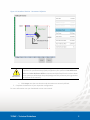
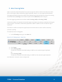
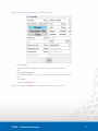
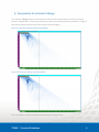
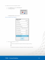
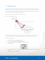
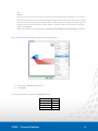
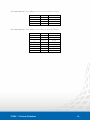
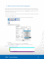
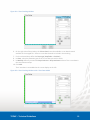
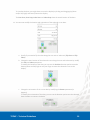
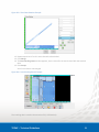
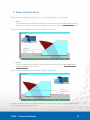
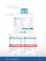
TOPAZ
TM
Technical Guidelines – Release 3.7R21
TOPAZ is one of the most efficient and
versatile non-destructive testing (NDT)
instrument. Simply brilliant!
www.zetec.com
Table of Content
Table of Content ........................................................................................................................................... 2
1.
PaintBrush Scanner Support ................................................................................................................. 3
2.
Auto-Crossing Gates.............................................................................................................................. 6
3.
Probe Position Marker .......................................................................................................................... 7
4.
Interpolation for Volumetric Merge ..................................................................................................... 9
5.
Compound Scan .................................................................................................................................. 11
6.
Path Correction for Pitch-&-Catch Configuration ............................................................................... 15
7.
TCG Auto Calibration........................................................................................................................... 16
8.
C-Scan Stitching................................................................................................................................... 17
9.
Wedge Definition Mode...................................................................................................................... 22
TOPAZ – Technical Guidelines
2
1. PaintBrush Scanner Support
NDT PaintBrush™ is a hand held scanner with dual encoder design that allows free motion on a scanindex inspection canvas. Not bounded by single axis motion, it allows you to freely paint over the
surface to examine for enhance wall thickness measurements. NDT PaintBrush features were integrated
to the TOPAZ™ and now available in UltraVision through the touch interface.
To create an inspection configuration with your PaintBrush scanner:
1. Start-up your TOPAZ
2. Connect the encoder feedback cable of the PaintBrush scanner to your TOPAZ;
A window will pop-up showing the detection process.
3. Define your specimen;
4. To define your PaintBrush inspection sequence, go to the Mechanical menu:
a. In the Sequence tab, select PaintBrush;
Figure 1-1 PaintBrush Sequence Selection
b. For the Scan and Index-axis, define the Start, Stop and Resolution of the inspection
sequence;
c. In the PaintBrush tab, click Position
The PaintBrush Position window appears.
TOPAZ – Technical Guidelines
3
Figure 1-2 PaintBrush Position Window
d. In the PaintBrush Position window (refer to Figure 1-3):
i. Define the Fork Offset if different than default.
When PaintBrush is connected, the Fork Offset value is set automatically. The
Fork Offset value is the length of the probe holder (from the front of the
scanner to the rotation point of the wedge).
ii. Define the Orientation Preset.
Orientation of the scanner according to the scan and index axes
iii. Define the Scan Preset.
Distance between the scanner reference point and the origin of scan/index
coordinate system along the scan axis.
iv. Define the Index Preset.
Distance between the scanner reference point and the origin of scan/index
coordinate system along the index axis.
v. You can also move the PaintBrush on the display by tapping on any corner or
rotate it by tapping directly on it.
TOPAZ – Technical Guidelines
4
Figure 1-3 PaintBrush Position - Parameters Definition
IMPORTANT
It is important that your defined positioning is exactly where you will start your
inspection for your data to be properly mapped on your specimen. Scan Reference
Offset and Index Reference Offset are automatically defined from the values above.
These values are defined per the probe/wedge assembly reference point (green dot
on the front of the scanner).
e. Click Accept once the start location and orientation are correctly defined.
5. Complete the definition of your inspection configuration.
For more information see your PaintBrush scanner user manual.
TOPAZ – Technical Guidelines
5
2. Auto-Crossing Gates
Gates are used to extract information from an A-scan signal in order to create C-scan data, turn ON or
OFF an alarm signal, obtain information (signal amplitude, location...) or set a signal synchronization.
The trigger parameter allows you to define if the detection gate data will take into account the crossing
threshold location (Crossing) or the maximum peak location (Maximum) within the gate.
Two new triggering modes have now been added: Crossing (-6dB) and Crossing (-12dB).
In these two modes, the detection threshold changes according to the maximum amplitude of the signal
within the gate. Threshold is automatically adjusted at -6dB or -12dB from the live maximum signal
amplitude.
This feature is useful to compensate signal response variations due to uneven surfaces caused by
corrosion or pitting.
To implement auto-crossing gates:
1. In the UT Settings menu, go in the Gates tab.
Figure 2-1 UT Settings menu - Gates Tab
2. Click Trigger.
3. Select Crossing (-6dB).
To adjust the automatic threshold setting to -6dB from the maximum signal amplitude.
OR
Select Crossing (-12dB).
To adjust the automatic threshold setting to -12dB from the maximum signal amplitude.
Your detection is now set in auto-crossing mode.
TOPAZ – Technical Guidelines
6
3. Probe Position Marker
The probe position marker is a live cursor that displays the probe’s position in real time during the
inspection. It provides a reliable and constant visual feedback for encoded scanning sequences and is
the perfect tool to ensure complete examination coverage when using your PaintBrush™ scanner.
The probe cursor is displayed as a pink marker in your volumetric views (Top, Side and End).
Figure 3-1 Probe Cursor on VC-Top (C) Display for a Focal Law at 60°
Probe Cursor
The orientation and length of the Probe cursor, in the displayed view, is computed based on the
selected focal law beam orientation (refracted and skew angles). By default, the probe cursor is always
displayed in your Top, Side and End views.
To change the Probe cursor properties:
1. Click on the desired view (Top, Side or End) to display the View Settings toolbar.
2. Click View Properties.
The View Properties window appears
3. Select Probe Cursor to display the different parameter options.
TOPAZ – Technical Guidelines
7
Figure 3-2 View Properties Window - Probe Cursor Options
4. Select Always.
To always display the Probe cursor (in setup and acquisition mode).
OR
Select Acquisition Only.
To display the Probe cursor only during data acquisition (acquisition mode).
OR
Select Hide.
To hide the Probe cursor.
You can now adjust the Probe cursor settings to better fit your application.
TOPAZ – Technical Guidelines
8
4. Interpolation for Volumetric Merge
The volumetric Merge function now includes the use of sectorial interpolation, which fills the empty
spaces in merged views. Those empty spaces are a typical result when performing volumetric merges of
data acquired with azimuthal focal laws (multiple refracted angles).
Figure 4-1 Volumetric Merge without Interpolation
Figure 4-2 Volumetric Merge with Interpolation
This interpolation is applied by default to the volumetric merge process.
TOPAZ – Technical Guidelines
9
To modify the use of the interpolation option:
1. In the Analysis menu, go to Processing tab.
2. Click Merge Custom.
The Merge Custom window appears.
Figure 4-3 Merge Custom Window
3. Click Use Interpolation to select:
Yes
To use the interpolation during the volumetric merge processing.
OR
No
To disable the interpolation during the volumetric merge processing.
TOPAZ – Technical Guidelines
10
5. Compound Scan
Compound scanning is a combination of azimuthal and linear focal laws in one channel configuration.
The end result is to create a sweep that has a greater coverage than what traditional linear or azimuthal
scans are able to offer. With compound focal laws, the refracted angle of the beam changes from one
aperture to the next within your phased array transducer.
The following figure shows an example of compound scanning.
Figure 5-1 Compound Scan Example
Aperture Motion
(Linear Scanning)
70°
40°
Refracted Angle Sweep
(Azimuthal Scanning)
As illustrated, the desired refracted angles are distributed on the different apertures defined by the
linear focal laws parameters and therefore defines the angular resolution between each beam.
To define a compound scan:
1.
2.
3.
4.
Define your specimen (see Specimen menu).
In the Channel menu, go to the Configuration tab.
Ensure that the right probe and wedge combination is selected.
Click Calculator.
5. In the Calculator Window, define your Skew Angle, Scan Reference, Index Reference and Wave
Type.
6. Click Sweep and select Compound.
TOPAZ – Technical Guidelines
11
Figure 5-2 Setting Sweep Parameter to Compound
The parameter list of the Calculator window is adjusted.
Figure 5-3 Calculator Window for Compound Focal Laws (Sparse)
7. Define Beam Density:
Sparse
(See Figure 5-3) Each law is an increment on the linear sweep and on the angle sweep. This
means that the exit point moves and the refracted angle changes between each laws. The angle
range, defined by Start Angle and Stop Angle, is evenly distributed over all exit points.
Therefore the angular resolution is automatically set by dividing the angular range by the total
number of apertures.
Motion of the aperture is defined by the Aperture, First Element and Last Element parameters.
TOPAZ – Technical Guidelines
12
OR
Dense
Each law is an increment on the linear sweep or on the angle sweep in alternation. This means
that the exit point move or the refracted angle change between each laws. This creates a sweep
that is denser than the sparse compound sweep. It also provides a sweep with density similar or
better than traditional Azimuthal or linear sweep. The total number of focal laws is two times
higher when Sparse.
Motion of the aperture is defined by the Aperture, First Element and Last Element parameters.
Figure 5-4 Calculator Window for Compound Focal Laws (Dense)
8. Set all others Calculator parameters.
9. Click Accept.
Focal law specification example for Compound sweep:
Start Angle
Stop Angle
Aperture
First Element
Last Element
TOPAZ – Technical Guidelines
40 deg.
70 deg.
16
1
19
13
When Beam Density is set to Sparse, the focal laws are defined as follows:
Focal Law Id
1
2
3
4
Aperture
1 to 16
2 to 17
3 to 18
4 to 19
Refracted Angle
40.00°
50.00°
60.00°
70.00°
When Beam Density is set to Dense, the focal laws are defined as follows:
Focal Law Id
1
2
3
4
5
6
7
8
TOPAZ – Technical Guidelines
Aperture
1 to 16
1 to 16
2 to 17
2 to 17
3 to 18
3 to 18
4 to 19
4 to 19
Refracted Angle
40.00°
47.50°
47.50°
55.00°
55.00°
62.50°
62.50°
70.00°
14
6. Path Correction for Pitch-&-Catch Configuration
When using a Pitch-&-Catch inspection configuration with 0 degree linear sweep, the ultrasound true
depth scale has now a correction that takes into account your probe separation and probe configuration
(wedge and roof angle, etc.). This new ultrasound axis scale, True Depth PC, is available for the A-scan,
VC-Side (B) and VC-End(D) display.
This feature is available for linear focal laws in pitch-&-catch configuration with a 0°LW inspection angle.
To display the True Depth PC ruler:
1. Click on the desired view (Top, Side or End) to display the View Settings toolbar.
2. Click View Properties.
The View Properties window appears
3. Click Usound and Select True Depth PC.
4. Click Close.
The selected view’s ultrasound axis is now set to True Depth PC.
The True Depth PC ruler is purple and the scale reflects the depth correction.
Figure 6-1 True Depth PC Ruler Example
TOPAZ – Technical Guidelines
15
7. TCG Auto Calibration
The TCG Auto calibration allows you to create multiple TCG points in one single scan, using one
detection gate with the appropriate start and range to cover all reflectors.
To create a TCG using the TCG Auto feature:
1. Go to the Calibration menu and select TCG Auto.
The TCG Auto Calibration menu appears.
2. In Parameters tab, set:
a. Reflector Type
b. Detection gate Threshold
c. Signal amplitude Target
d. Verification Tolerance for signal amplitude
e. Detection Blanking
It defines the minimum distance between the reflectors in true depth.
3. In Calibrate tab, set:
a. Set Sector
b. Set Start and Range of the detection gate.
Ensure that these values allows the detection gate to cover all reflectors
4. Scan the reflectors by moving your probe over your calibration specimen.
5. Click Compute.
All your TCG point are now created.
Figure 7-1 TCG Auto Calibration
TOPAZ – Technical Guidelines
16
8. C-Scan Stitching
When performing the examination of large surfaces, it is sometimes useful to divide your zone coverage
in several inspection patches, i.e. creating multiple data files, for a more efficient site deployment.
When acquiring C-scan data you can merge those signals into one consolidated file and easily
reconstruct the entire inspection, i.e. creating a complete mapping of the examined surface.
The C-Scan Stitching feature allows you to adjust the position of the data on the surface and correct
angular misalignment that might have occurred during the scanning process.
To perform C-Scan Stitching:
1. Perform a File Merge:
a. In the Analysis menu, click File Merger.
b. In the File to merge window, click Add.
c. In the Select file to merge window, identify the files to merge.
d. Select one file and click Accept.
e. Repeat steps 1.b to 1.d until all relevant files are selected.
f. In the File to merge window, review the selected file names.
g. Click Merge.
TOPAZ – Technical Guidelines
17
h. In the File Merger window, enter a name for the merged data file.
i.
Click Accept.
The merged file is now created with the different original files being divided in different
channels in the new file. The next step is to perform the stitching process.
2. In the File menu, click Open Data.
3. In the Open Data window, browse to find the DataFileMerger directory.
4. Select the appropriate merged file and click Accept.
5. In the Analysis menu, click C-Scan Stitching.
The C-Scan Stitching window appears.
TOPAZ – Technical Guidelines
18
Figure 8-1 C-Scan Stitching Window
6. On the right side of the window, the C-Scan data shows the available c-scan data channels
available in the merged file. Select a c-scan data channel to include in the stitching.
7. For the selected data, define the Data type (Amplitude or Position).
8. In Gates, select the detection gate of the C-scan data you wish to stitch.
9. In Method, define if you want to Keep minimum or Keep maximum values of the c-scan data in
the case of data overlap.
10. Click Add.
The C-scan data is now added to the c-scan display on the left.
Figure 8-2 C-Scan Stitching Window with C-Scan Data Added
TOPAZ – Technical Guidelines
19
To visualize the data, you might have to move the display by clicking and dragging (up/down
and/or left/right) and zoom/unzoom the display.
The Scan Start, Scan Stop, Index Start and Index Stop show the actual location of the data.
11. You can now modify the location and orientation of the selected c-scan data.
a. Specify if you need to flip the data along the scan-axis or index-axis (Flip Scan and Flip
Index).
b. Change the start location of the selected c-scan along the scan and index axes by modify
the Scan and Index parameters.
To modify the location of the data, you can use the Position direction-pad to move the
data up/down and left/right or use your finger to move the selected c-scan on the
display.
c. Change the orientation of the c-scan data by modifying the Rotate parameter (in
degrees).
To modify the orientation of the data, you can use the Rotation pad to turn the selected
data clockwise or counter-clockwise.
TOPAZ – Technical Guidelines
20
Figure 8-3 C-Scan Data Rotation Example
12. Repeat steps 6 to 11 for all c-scan channels to be stitched.
13. Click Merge.
14. The New stitching name window appears, enter a name for the new channel with the stitched
data.
15. Click Accept.
Your C-scan data is now merged.
Figure 8-4 C-scan Stitching Result Example
The resulting data is saved in the extension file (.UVExtension).
TOPAZ – Technical Guidelines
21
9. Wedge Definition Mode
When defining your wedge characteristics, you now have two different modes available:

Legacy:
This mode allows you to define the height of the first element using the back left corner of the
wedge as the reference. Historically, this mode was the one used in previous software release.
Figure 9-1 Legacy Wedge Definition Example - Height of First Element

Default:
This new mode allows you to define the height of the first element using the middle of the
wedge front edge as the reference.
Figure 9-2 Default Wedge Definition Example - Height of First Element
For plate examination, there is no difference between the two modes, this only affects wedge definition
for pipe-like or curved surface specimens.
TOPAZ – Technical Guidelines
22
To set the wedge definition mode:
1. In the Tools menu, select Options.
2. In the Options window, set the Wedge Definition Mode to Legacy or Default.
Figure 9-3 Options Window
3. Click Accept.
The Wedge Definition Mode is defined and will now on be used in the Wedge Editor.
TOPAZ – Technical Guidelines
23