1
5.10.9
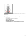
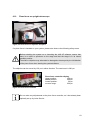
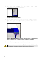
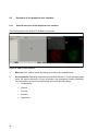
Mirror Housing
Front view of the mirror housing:
Figure 32: Safety label for mirror housing (top)
51
52
6. Safety Instructions for Operating the System
6.1
Requirements Related to the Installation/Storage Location
This device was designed for use in a lab and may not be set up in areas with
medical devices serving as life-support systems such as intensive-care wards.
This equipment is designed for connection to a grounded (earthed) outlet. The
grounding type plug is an important safety feature.
To avoid the risk of electrical shock or damage to the instrument, do not disable
this feature.
To avoid the risk of fire hazard and electrical shock, do not expose the unit to rain
or humidity.
Do not open the cabinet. Do not allow any liquid to enter the system housing or
come into contact with any electrical components. The instrument must be
completely dry before connecting it to the power supply or turning it on.
6.2
General Safety Instructions for Operation
Do not look into the eyepieces during the scanning operation.
Do not look into the eyepieces when switching the beam path in the microscope.
Never look directly into a laser beam or a reflection of the laser beam. Avoid all
contact with the laser beam.
Never deactivate the laser protection devices. Please read the chapter "Laser
Protection Devices" to familiarize yourself with the safety devices of the system.
53
Do not introduce any reflective objects into the laser beam path.
Be sure to follow the included operating instructions for the microscope.
6.3
Eye Protection
6.3.1
MP System with Upright Microscope
Wearing safety goggles (order number: 156502570) is compulsory. Appropriate
safety goggles for IR laser radiation are provided with the system when delivered.
These safety goggles do not offer any protection against visible laser radiation
(visible spectrum).
During the scanning operation, all persons present in the room must wear safety
goggles.
The IR laser beam can be deflected or scattered by the specimen or objects moved into the
specimen area. Therefore, it is not possible to completely eliminate hazards to the eye from
IR laser radiation.
The supplied safety goggles only provide safe protection against the infrared lasers supplied
by Leica Microsystems CMS GmbH.
6.3.2
MP System with Inverted Microscope
It is not necessary to wear eye protection. If the device is used as prescribed and the safety
instructions are observed, the limit of the laser radiation is maintained so that eyes are not
endangered.
6.3.3
VIS and UV Systems with Inverted or Upright Microscope
It is not necessary to wear eye protection. If the device is used as prescribed and the safety
instructions are observed, the limit of the laser radiation is maintained so that eyes are not
endangered.
54
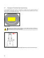
6.4
Specimen Area
The light of all employed VIS lasers used (wavelength range 400 - 700 nm, visible spectrum
) and UV lasers (wavelength range < 400 nm, invisible) is fed through a fiber optic cable and,
therefore, completely shielded until it leaves the microscope objective and reaches the
specimen. The beam divergence, depending on the objective used, is up to 1.16 rad.
Figure 33: Specimen area of upright and inverted microscope
During the scanning operation, the laser radiation is accessible after exiting the
objective in the specimen area of the laser scanning microscope.
This circumstance demands special attention and caution. If the laser radiation
comes in contact with the eyes, it may cause serious eye injuries. For this reason,
special caution is absolutely necessary as soon as one or more of the laser
emission warning indicators are lit.
If the system is used as prescribed and the safety instructions are observed during
operation, there are no dangers to the operator. Always keep your eyes at a safe
distance of at least 20 cm from the opening of the objective.
55
6.5
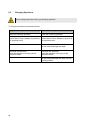
Changing Specimens
Never change specimens during a scanning operation.
To change specimens, proceed as follows:
Upright microscope
Inverted microscope
Finish the scanning operation.
Finish the scanning operation.
Ensure that no laser radiation is present in Ensure that no laser radiation is present in
the specimen area.
the specimen area.
Tilt the transmitted-light arm back.
Exchange the specimen.
Insert the specimen correctly into the
specimen holder.
Exchange the specimen.
Insert the specimen correctly into the
specimen holder.
Tilt the transmitted-light arm back into the
working position.
56
6.6
Changing Objectives
Do not change objectives during a scanning operation.
To change objectives, proceed as follows:
1. Finish the scanning operation.
2. Switch off the internal lasers using the detachable-key switch.
3. If any external lasers are present, switch them off with their detachable-key switch
or as described in the operating manual of the laser manufacturer.
4. Rotate the objective nosepiece so that the objective to be changed is swiveled out
of the beam path and points outward.
5. Exchange the objective.
All unoccupied positions in the objective nosepiece must be closed using the
supplied caps.
For MP systems, dry objectives (air objectives) may not be used with a numerical
aperture (NA) larger than 0.85. This does not apply to immersion objectives (oil,
water).
If a piezo focus is installed in your system, please also observe the safety notes
related to changing objectives with a piezo focus in 6.10.1.
57
6.7
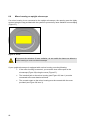
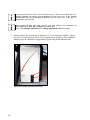
Changing the Transmitted-Light Lamp Housing
If no transmitted-light lamp housing is connected, to protect from the potential escape of
laser radiation, the opening (Figure 35 or Figure 36) must be securely sealed with the cover
(Figure 34) that accompanies the system.
Figure 34: Cover
To prevent the emission of laser radiation, do not switch the lasers on without a
lamp housing or cover on the microscope.
Figure 35: Port for connecting the transmitted-light lamp housing on the inverted microscope
58
Figure 36: Port for connecting the transmitted-light lamp housing or mirror housing on the
upright microscope
If your microscope features a transmitted-light lamp housing that you would like to replace,
proceed as follows:
1. Switch off the lasers.
2. Disconnect the lamp housing from the power supply.
3. Remove the lamp housing.
4. Modify the lamp housing as needed.
5. After finishing the tasks, screw the new lamp housing back onto the microscope.
59
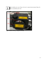
6.8
Mirror housing on upright microscope
If a mirror housing is not connected to the upright microscope, the opening must be tightly
covered using the cap provided with the system to prevent any laser radiation from escaping
(Figure 37).
Figure 37: Cover
To prevent the emission of laser radiation, do not switch the lasers on without a
mirror housing or cover on the microscope.
If your upright microscope is equipped with a mirror housing, note the following:
60
•
If the mirror housing is removed, you must the close off the port on the
microscope (Figure 36) using the cover (Figure 37).
•
The interlock jack on the mirror housing (see Figure 38, item 1) must be
connected to the scan head at all times.
•
The unused output on the mirror housing must be covered with the cover
provided (see Figure 38, item 3).
When installing the cover (Figure 38, item 3), ensure that the button (Figure 38,
item 2) is pressed by the cover.
Figure 38: Mirror housing on upright microscope
61
6.9
Changing Filter Cubes, Beam Splitters or Condenser
Do not change any filter cubes or beam splitters during a scanning operation.
In LAS AF, set the operating voltage of all external detectors to 0 V and disable
them using the checkbox. If the detectors are not de-energized, they could be
damaged by the infiltration of ambient light.
To change filter cubes or beam splitters proceed as follows:
Upright microscope
Inverted microscope
Finish the scanning operation.
Finish the scanning operation.
In LAS AF, set the operating voltage of all
external detectors to 0 V.
In LAS AF, set the operating voltage of all
external detectors to 0 V.
Remove the cover of the fluorescence
module
(see operating manual for microscope).
Pull out the fluorescence module.
Remove the filter cube/beam splitter.
Remove the filter cube/beam splitter.
Insert the desired
filter cube/beam splitter.
Insert the desired
filter cube/beam splitter.
Reattach the cover to the front of the
fluorescence module.
Reinsert the fluorescence module.
Never disconnect a fiber optic cable.
Never remove the scanner from the microscope during operation.
Before removing the scanner, the system must be completely switched off.
Do not use an S70 microscope condenser. The large working distance and the low
numerical aperture of the S70 microscope condenser could pose a hazard due to
laser radiation. Therefore, only S1 and S28 Leica microscope condensers should
be used.
62
6.10
Piezo focus on upright microscope
Figure 39: Piezo focus on objective nosepiece
If a piezo focus is installed on your system, please also observe the following safety notes:
Before switching the system on or launching the LAS AF software, ensure that
there is no slide or specimen on the stage and that the stage is in its lowest
possible position.
The slide or objective may otherwise be damaged or destroyed by the initialization
of the piezo focus when starting the system/software.
The objective can be moved by 150 µm in either direction. The total travel is 300 µm.
Piezo focus controller display:
Upper position:
350 µm
Middle position:
200 µm
Lowest position:
50 µm
xz-scan range:
250 µm
Figure 40: Piezo focus controller
Do not make any adjustments to the piezo focus controller, as it has already been
optimally set up by Leica Service.
63
Figure 41: Spacer on objective
Please note that the focus position of an objective with piezo focus is 13 mm lower
than those without piezo focus. A spacer (Figure 41) is installed on all other
objectives to ensure the same focal plane.
6.10.1
Objective Change with Piezo Focus Configuration
Do not change objectives automatically! The automatic motion may damage the
cable of the piezo focus.
In addition to the regular procedure (see chapter 6.6) the stage must be lowered
as much as possible and the slide or specimen must be removed from the stage
before changing the objective on the piezo focus. The slide or objective may
otherwise be damaged or destroyed by the initialization of the piezo focus when
starting the system/software.
When replacing the objective on the piezo focus, you must perform a teach-in for
the new objective in LAS. Please see the instructions on this topic in the
microscope operating manual.
64
7. Starting Up the System
7.1
Switching On the System
With the motorized stage (156504145) for DMI 6000 (inverted):
Before the system start or start of the LAS AF, the illuminator arm of the inverted
microscope must be swung back, because the motorized stage can be initialized
and damage the condenser.
With the motorized stage (156504155) for DM 6000 (upright):
Before the system start or start of the LAS AF, the stage must be moved
downwards, because during initialization, it can come into contact with the
objective nosepiece and damage the objectives.
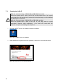
1. Switch on the workstation (PC switch) at the main switch board.
Figure 42: Switching on the workstation
You do not have to start the operating system—it starts automatically when you
switch on the computer. Wait until the boot process is completed.
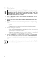
2. Log on to the computer. After you simultaneously press the Ctrl, Alt, and Del
keys, the logon information dialog box appears.
65
Use your personal user ID if one has been set up. This ensures that the userspecific settings are saved and maintained for this user only. If the system
administrator has not yet assigned a personal user ID, log on as "TCS_User". A
password is not required.
After logging on with your own user ID, you may change your password by
pressing the keys Ctrl, Alt, and Del at the same time.
Then, click Change password. The Change password dialog box opens.
3. Check whether the microscope is switched on. If the readiness indicator (Figure
43, item 1) on the electronic box is lit, the microscope is operating. If the readiness
indicator is not lit, activate the toggle switch (Figure 432) of the electronic box.
Figure 43: Switching on the microscope
66
4. Switch on the scanner on the main switch board.
Figure 44: Turning on the scanner
5. Switch on the lasers on the main switch board.
Figure 45: Switching on the lasers
The power supplies and fan of the system have been started.
67
The power supply of the achromatic light laser is started if the main power switch
on the rear side of the achromatic light laser is set to "On".
6. To switch on the lasers in the supply unit, activate the detachable-key switch on
the main switch board (see Figure 46).
Figure 46: Activating the detachable-key switch
7. To switch on the achromatic light laser, activate the detachable-key switch at the
front of the achromatic light laser (see Figure 47) 5.
Figure 47: Detachable-key switch for the achromatic light laser
From this time on, laser radiation may be present in the specimen area of the laser
scanning microscope. Follow the safety instructions provided in Chapter 6 Safety
Instructions for Operating the System.
5
Applies only to the TCS SP5 X system.
68
If the room temperature exceeds 40°C, the white light laser switches off. An error
report appears in the display of the white light laser. The white light laser cannot
be switched on again until the room cools off.
Shocks to the white light laser can cause an error message in the display of the
white light laser. Switch the white light laser off, then on again after 10 seconds.
8. To switch on the external UV laser, activate the key switch on the front of the
power supply (see)6.
Figure 48: Key switch for the external UV laser
From this time on, laser radiation may be present in the specimen area of the laser
scanning microscope. Follow the safety instructions provided in Chapter 6 Safety
Instructions for Operating the System.
For switching off the system, refer to Chapter 8 Switching Off the System.
6
Applies only to systems with an external UV laser.
69
7.2
Starting the LAS AF
With the motorized stage (156504145) for DMI 6000 (inverted):
Before the system start or start of the LAS AF, the illuminator arm of the inverted
microscope must be swung back, because the motorized stage can be initialized
and damage the condenser.
With the motorized stage (156504155) for DM 6000 (upright):
Before the system start or start of the LAS AF, the stage must be moved
downwards, because during initialization, it can come into contact with the
objective nosepiece and damage the objectives.
1. Click the LAS AF icon on the desktop to start the software:
Figure 49: LAS AF icon on the desktop
2. Select whether the system should be operated in resonant or non-resonant mode.
Figure 50: Resonant or non-resonant mode
70
3. Start the LAS AF by clicking the "OK" button.
Figure 51: LAS AF start window
You are now in the main view of the LAS AF.
Figure 52: LAS AF main view7
7
Display may differ based on the system configuration.
71
7.3
Setting Up Users
The default user name for the system is "TCS_User". No default password is set.
It is recommended to set up a separate user ID for each user (set up by the
system administrator). This will create individual directories that can be viewed by
the respective user only. Since the LCS AF software is based on the user
administration of the operating system, separate files are created for managing
user-specific profiles of the LCS AF software.
1. Log on as administrator. To do so, use the username (ID) "Administrator" and the
password "Admin"
2. Open the User Manager. Select: Start / Programs / Administrative Tools / User
Manager.
3. Define a new user. Enter at least the following information in the open dialog
window:
•
User ID
•
Password (must be re-entered in the next line for confirmation purposes)
4. Select the following two check boxes:
•
User must change password at next logon (this allows the new user to
define his or her own password at logon)
•
Password never expires (this allows a defined password to be valid until
either it is changed in the User Manager or the user is deleted)
5. Select the Profiles option in the bottom section of the dialog. In the Local path
field, enter the following path for storing the user-specific file: d:\users\username
("username" is a wildcard which must be replaced by the currently defined user
name.)
Factory-installed hard disk drives are provided with two partitions (C:\ and D:\). Set
up the user directory on partition D:\.
72
8. Switching Off the System
The switch-off sequence must be followed! If the switch-off sequence listed below
is not followed, the lasers could be damaged!
1. Save your image data: On the menu bar, select File → Save as to save the data
record.
2. Close the LAS AF: On the menu bar, select File → Exit. Exit the LAS AF.
3. On the main switch board, switch off the lasers in the supply unit using the
detachable-key switch (Figure 56, item 2). The emission warning indicator (Figure
56, item 1) goes out.
4. Switch off the achromatic light laser with the detachable-key switch (see Figure 53)
on the front of the achromatic light laser. The emission warning indicator goes out.
8
Figure 53: Detachable-key switch for the achromatic light laser
5. Switch off the external UV laser with the key switch (see Figure 54). The emission
warning indicator goes out. 9
Figure 54: Key switch for the external UV laser
8
9
Applies only to the TCS SP5 X system.
Applies only to systems with an external UV laser.
73
6. Shut
down
the
computer.
On
the
→ Shutdown to shut down the TCS workstation.
toolbar,
select
Start
Figure 55: Shutting down the computer
7. Next, turn off the switches on the main switch board for the TCS workstation
(Figure 56, item 5), the scanner (Figure 56, item 4) and the laser (Figure 56, item
3).
Figure 56: Main switch board (1 = emission warning indicator, 2 = detachable-key
switch, 3 = switch for laser, 4 = switch for scanner, 5 = switch for workstation)
8. Switch off the microscope and any activated fluorescence lamps.
If your system features external lasers (IR, UV or others), switch them off in
accordance with the respective operating manual from the manufacturer.
74
9. Introduction to LAS AF
9.1
General
The LAS AF software is used to control all system functions and acts as the link to the
individual hardware components.
The "experiment concept" of the software allows for managing the logically interconnected
data together. The experiment is displayed as a tree-structure in the software and features
export functions to open individual images (JPEG, TIFF) or animations (AVI) in an external
application.
9.2
Online Help
9.2.1
Structure of the Online Help
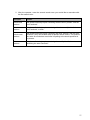
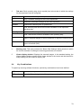
The online help is divided into 4 main chapters:
Books
Contents
General
Contains legal notices and general information on the
LAS AF.
LAS AF Online Help
Contains general information for the LAS AF online help.
Dialog descriptions
Contains detailed descriptions of the dialogs in the LAS
AF user interface.
Additional information
Contains background information on LAS AF and
application-related topics, such as digital image
processing and dye separation.
75
9.2.2
Accessing the Online Help
The online help can be accessed in three ways:
In the respective context (context-sensitive)
Via the Help menu
With the key combination CTRL + F1
In the respective context (context-sensitive)
Click the small question mark located in the top right corner of every dialog window.
Online help opens directly to the description for the corresponding function.
Via the Help menu
Click the Help menu on the menu bar. The menu drops down and reveals search-related
options, including the following:
Contents
This dialog field contains the table of contents in the form of a directory
tree that can be expanded or collapsed.
Double-click an entry in the table of contents to display the
corresponding information.
Enter the term to be searched for. The online help displays the keyword
that is the closest match to the specified term.
Index
Select a keyword. View the corresponding content pages by doubleclicking the key word or selecting it and then clicking the Display button.
Search
Enter the term or definition you want to look up and click the LIST
TOPICS button. A hierarchically structured list of topics is displayed.
About
Opens the User Configuration dialog box, where you can, for example,
select the language in which the online help is shown.
9.2.3
Full-text Search with Logically Connected Search Terms
Click the triangle to the right of the input field on the Search tab to view the available logical
operators.
1. Select the desired operator.
76
2. After the operator, enter the second search term you would like to associate with
the first search term:
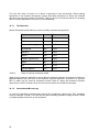
Examples
Results
Pinhole and
sections
This phrase finds help topics containing both the word "pinhole" and the
word "sections".
Pinhole or
sections
This phrase finds help topics containing either the word "pinhole", the
word "sections", or both.
Pinhole near
sections
This phrase finds help topics containing the word "pinhole" and the word
"sections" if they are located within a specific search radius. This method
also looks for words that are similar in spelling to the words specified in
the phrase.
Pinhole not
sections
This phrase finds help topics containing the word "pinhole", but not
containing the word "sections".
77
9.3
Structure of the graphical user interface
9.3.1
General Structure of the Graphical User Interface
The user interface of the LAS AF is divided in five areas:
Figure 57: LAS AF user interface
1
Menu bar: The various menus for calling up functions are available here.
2
Arrow symbols: Operating steps with the individual functions. These operating steps
mirror the typical sequence of scan acquisition and subsequent image processing.
The functions are grouped correspondingly into these operating steps.
78
•
Configuration
•
Acquire
•
Process
•
Quantify
•
Application
3
Tab area: Each operating step (arrow symbol) has various tabs in which the settings
for the experiment can be configured.
Acquire
Experiments: Directory tree of opened files
Setup: Hardware settings for the current experiment
Acquisition: Parameter settings for the scan acquisition
Process
Experiments: Directory tree of opened files
Tools: Directory tree with all the functions available in the respective
operating step
Quantify
Experiments: Directory tree of opened files
Tools: Tab with the functions available in this operating step
Graphs: Graphical display of values measured in regions of interest (ROI)
Statistics: Display of statistical values that were determined in the plotted
regions of interest (ROI)
4
Working area: This area provides the "Beam Path Settings" dialog window in which
the control elements for setting the scanning parameters are located.
5
Viewer display window: Displays the scanned images. In the standard setting, the
Viewer display window consists of the image window in the center and the buttons for
image editing (5a) and channel display (5b).
9.4
Key Combinations
To speed up recurring software functions, special key combinations have been defined:
CTRL + N
Opens a new experiment
CTRL + O
Starts the "Open dialog window" for opening an existing file.
79
80
10. Introduction to Confocal Work
10.1
Preparation
The following sections describe a number of basic procedures that cover most of the tasks
related to the instrument.
a) Upright microscope
1 Objective
2 Cover slip
3 Seal
4 Specimen slide
5 Stage focus
b) Inverted microscope
1 Embedding
2 Specimen
3 Immersion
4 Lens focus
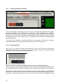
Figure 58: Arrangement of cover slip and specimen on an upright microscope (a) and inverted
microscope (b). When using objectives with cover slip correction, ensure that the cover slip
(i.e. the top side of embedded specimens) is facing down.
Background information has also been provided to explain the reasons behind various
settings. These are not descriptions of the individual functions and controls of the instrument
and graphical user interface, but an informative tour of the essential tasks that is designed to
remain valid even if future upgrades change the specific details of operating the instrument.
81
The very first step, of course, is to place a specimen in the microscope. When placing
specimens in an inverted microscope, ensure that fixed specimens on slides are inserted
with the cover slip facing down (Figure 58). Failing to do so is a frequent reason for not being
able to find the specimen or focus on it in the beginning.
10.1.1
The Objective
Select the objective with which you want to initially examine the specimen.
Medium
Table 3
Refractive Index
Water
Imm
1,333
PBS
Emb
1,335
Glycerol 80 % (H2O)
Imm
1,451
Vectashield
Emb
1,452
Glycerol
Imm
1,462
Moviol
Emb
1,463
Kaisers Glycerol Gel
Emb
1,469
Glass
Mat
1,517
Oil
Imm
1,518
Canada Balsam
Emb
1,523
Table of various immersion media
When using immersion objectives, ensure that an adequate quantity of immersion medium is
applied between the front lens of the objective and the specimen. Immersion oil, glycerol
80% or water may be used as immersion media (Table 3). Apply the immersion medium
generously, but be sure that it does not flow into the stand of inverted microscopes.
10.1.2
Conventional Microscopy
To view the specimen conventionally through the eyepieces, ensure that "VIS" operating
mode is selected. "SCAN" is for use with the laser scanning operation image process. Select
a suitable position and focus on the specimen.
82
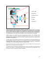
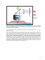
1 Filter cube
2 Specimen
3 Objective lens
4 Shutter
5 Lamp
6 Eyepiece
Figure 59: Incident light fluorescence scheme: light from a mercury lamp is collimated,
selected spectrally via an excitation filter and applied to the specimen via a color splitter
mirror. A shutter permits the specimen to be darkened. The emission (longer wavelength than
the excitation) is visible through the color splitter mirror and emission filter via the eyepiece.
The excitation filter, color splitter mirror and emission filter are grouped in a filter cube.
Optical sections are created using the transmitted-light method. Your specimen must
therefore reflect or fluoresce. Fluorescent specimens are most common. In many cases,
specimens with multiple dyes will be examined. Reflective specimens can also provide
interesting results, however.
The filter cubes (Figure 59) that correspond to the fluorescence must be positioned within the
beam path when viewing the specimen via the eyepieces. For more information on selecting
fluorescence filter cubes, please refer to the Leica fluorescence brochure or contact your
Leica partner. For a selection of filter cubes, see Table 4 below.
As specimen fluorescence can fade quickly, always close the shutter of the mercury lamp
when you are not looking into the microscope.
To switch to scan mode, press the appropriate keys on the microscope or use the switching
function in the software. The switching function may vary according to the motorization of the
microscope. Please consult help for more information.
83
Filter cube
Excitation filter
Dichroic
mirror
Emission filter
A
BP 340-380
400
LP 425
B/G/R
BP 420/30
415
BP 465/20
B/R
420/20;530/45
435;565
465/30;615/70
BFP/GFP
BP 385/15
420
BP 460/20
CFP
BP 436/20
455
BP 480/40
D
BP 335-425
455
LP 470
E4
BP 436/7
455
LP 470
FI/RH
BP 490/15
500
BP 525/20
G/R
BP 490/20
505
BP 525/20
GFP
BP 470/40
500
BP 525/50
H3
BP 420-490
510
LP 515
I3
BP 450-490
510
LP 515
K3
BP 470-490
510
LP 515
L5
BP 480/40
505
BP 527/30
M2
BP 546/14
580
LP 590
N2.1
BP 515-560
580
LP 590
N3
BP 546/12
565
BP 600/40
Y3
BP 545/30
565
BP 610/75
Y5
BP 620/60
660
BP 700/75
YFP
BP 500/20
515
BP 535/30
Table 4
Selection of filter cubes for Leica research microscopes and associated filter
specifications.
84
10.1.3
Why Scan?
Specimens must be illuminated over the smallest possible area to achieve a true confocal
image—this is essential to attaining truly thin optical sections.
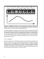
This has been achieved when the illumination spot is diffraction-limited; i.e. it cannot be
made physically smaller. The diameter of such a diffraction-limited spot corresponds to
dB=1.22*ë/NA, with ë representing the excitation wavelength and NA the numerical aperture
of the objective used (Figure 61).
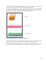
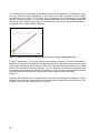
Figure 60: Illustration of the raster scan. Two mirrors move the illumination spot in x and y
directions across the specimen in rows so that the entire image can be reconstructed in
parallel.
To create a two-dimensional image, the spot must be moved over the entire surface and the
associated signal recorded on a point-by-point basis.
This is performed in a raster process similar to that of SEM instruments or the cathode ray
tubes still used in computer monitors and televisions (Figure 60). In a confocal microscope
with point scanners, the movement is realized by two mirrors mounted on so-called
galvanometric scanners. These scanners have the same design as electric motors; their
rotors are fixed at their base to the housing. Applying power to the scanner rotates the axis;
the rotation ceases at the point at which the torsional force and the electromagnetic force
balance. The mirror can thus be moved quickly between two angles by applying an
alternating voltage.
85
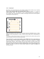
Figure 61: Smallest possible, diffraction-limited illumination spot (Airy disk). Below: an
intensity profile.
To scan a line, the x mirror must travel once across the field of view. The y mirror is then
moved a small amount, after which the x mirror then scans the next line. The signals from the
specimen are written to an image memory in synchronization and can be displayed on the
monitor.
10.1.4
How Is an Optical Section Created?
The term "confocal" is strictly technical and does not describe the effects of such an
arrangement. That will be described in greater detail here.
As already described in10.1.3, the illumination of the specimen is focused on the smallest
possible spot—hence the term "focal." The confocal design also involves an observation
point. The sensitivity distribution of the detector is reduced to a point by focusing light from
the specimen on a very small opening, known as the pinhole. This pinhole cuts off all
information not coming from the focal plane (Figure 62).
86
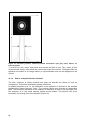
1
Out of
focus
2
in focus
3 Pinhole
(pinhole)
Figure 62: Creating an optical section using an incident-light process. Light not originating
from the focal plane is cut off by a spatial filter (here, a pinhole). Only information from the
focal plane can reach the detector.
The diaphragm thus acts as a spatial filter, but only when used with the correct, i.e. pointshaped, illumination.
As a rule, the optical section becomes thinner when the size of the pinhole is reduced. This
effect is reduced near the wavelength of the light used, and at a pinhole diameter of zero one
would theoretically receive the thinnest optical section for the wavelength and numerical
aperture used. A range apparently exists at 1 Airy which does not yet offer the thinnest
optical sections, but which is nevertheless very close to the theoretical limit. As the intensity
of the passing light increases roughly in proportion to the square of the pinhole diameter, it is
advisable not to close the pinhole too far to avoid excessive image noise. A value of 1 Airy is
a very good compromise and is selected automatically by the Leica TCS SP5. A dialogue is
available to set smaller or larger diameters if required. Playing with this parameter to study its
effects can be very worthwhile when you have the time.
87
10.2
Acquiring Optical Sections
Figure 63: Use the "Acquire" arrow key to acquire data in all Leica LAS AF applications.
The Leica TCS SP5 contains many functions in its user interface that reflect its wide range of
potential applications. The functions not needed for a given application are disabled,
however, to ensure efficiency and ease of use. Select the task at hand from the row of arrow
keys at the top. The functions required for data acquisition (the sole focus of these chapters)
are grouped under "Acquire" (Figure 63). For descriptions of the individual functions, please
see the online help.
This section will describe the aspects affecting the configuration of the most important
scanning parameters and special points that must be taken into consideration.
10.2.1
Data Acquisition
Press the "Live" button to begin data acquisition (Figure 64). Data will be transferred
continuously to video memory and displayed on the monitor. Initially, the data will not be
stored in a manner suitable for subsequent retrieval.
Figure 64: The "Live" button starts data acquisition in all Leica LAS AF applications.
This is a preview mode suitable for setting up the instrument. Stopping data acquisition will
also immediately stop the scanning operation, even if the image has not been fully rendered.
Alternatively, a single image can be captured. This image is then stored in the experiment
and can be retrieved later or stored on any data medium. Individual image scanning has the
advantage of exposing the specimen only once, but is less convenient if additional setup
88
work is required. Once all parameters are correctly set up, an image of the result may be
captured. Functions such as accumulation and averaging are supported.
The third data acquisition situation is the acquisition of a series in which the preselected
parameters are changed incrementally between scanning the individual images. Time series,
lambda series and z-stacks can be created in this manner (Figure 65).
Z-stack
Time series
Lambda series
Figure 65: Stack acquisition for 3D, time and lambda series
When using the instrument in "LiveDataMode", all captured images are automatically stored
with the time of capture. A preview mode is not available in that case (Figure 66).
This method is especially suitable for the observation of living objects over time while
changing the medium, applying electrical stimuli or executing changes triggered by light.
89
I (t)
t
Figure 66: LiveDataMode supports the continuous acquisition of data while changing setting
parameters, manipulating the specimen or performing bleaching sequences between the
individual scans. The clock continues running throughout the experiment and intensity
changes in regions of interest can be rendered graphically online.
The setting parameters for scanning a simple optical section are described and discussed
below. These settings are identical for all work with the instrument. Preconfigured parameter
sets have been stored in the software for typical specimen situations. You may also store
and recall custom parameter sets. The description below is based on the assumption that
you are using a specimen similar to the included standard specimen. The standard specimen
is a Convallaria majalis rhizome section with a histological fluorescent dye. The specimen
can be used for a wide range of fundamental problems and has the advantage that it
practically does not bleach.
10.2.2
Illumination
Laser lines suitable for the excitation of fluorescence may be selected as illumination. The
intensity of the laser line can be adjusted continuously using the line's slider. Moving the
slider all the way down disables the line. Using this slider, the intensity is adjusted
continuously via an acousto-optical tunable filter (AOTF). The intensity at which a sufficiently
noise-free image of the specimen can be obtained must be determined to reduce
deterioration of the specimen. Factors affecting this are the fluorescent dye, the line used,
the density of the dye in the specimen, the location and width of the selected emission band,
the scanning speed and the diameter of the emission pinhole.
90
Figure 67: Selecting the illumination intensity (1) via acousto-optical tunable filters (AOTF, 2)
and selecting the emission band in the SP detector (3).
If you select the "FITC" parameter set, the 488 nm argon line and a suitable band between
490 nm and 550 nm is set.
The entire beam path is represented graphically on the user interface. A spectral band with
the settings for the emission bands is located on the emission side. The laser line is visible at
the appropriate location in the spectrum as soon as a line is activated. When viewing the
specimen through the microscope, the light in the selected color will become lighter or darker
according to the position of the slider. If the laser scanning microscope is used as prescribed
and the safety instructions are observed, there are no dangers to the user's eyes. Always
keep your eyes at a safe distance of at least 20 cm from the opening of the objective. Read
the safety instructions in this user manual carefully.
If all of the other settings are in order, darker and lighter images will be visible on the monitor
when moving the slider for the illumination.
10.2.3
Beam Splitting
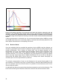
The simplest case would involve the selection of a laser line roughly at the maximum of the
excitation spectrum of a given fluorescent dye. This would achieve the best yield. In general,
however, lasers deliver much more light than necessary, and attenuation to 10% is generally
sufficient for good images (although that depends very strongly on the specimen's dye, of
course). One can thus also excite the fluorescence on the blue side of the excitation
maximum, which has the advantage of providing a wider band for the collection of the
emission (Figure 68).
91
Figure 68: Excitation spectrum of a fluorescent dye (blue) and emission spectrum (red). An
excitation in the maximum (Exc1) would result in only a narrow band to be collected on the
emission side (Em1). A significantly wider emission band (Em2) is available from an excitation
in the blue range, at which point the intensity of the laser can be increased without detrimental
effects.
A little experimentation is worthwhile here. An acousto-optical beam splitter (AOBS®) permits
all available laser lines to be conveniently added or removed without devoting attention to the
beam splitter characteristics or the spacing of the lines.
10.2.4
Emission Bands
Once the excitation light has reached the specimen via the AOBS® and the objective, an
emission is generated in the fluorescent molecules, the light of which is shifted toward longer
(redder) wavelengths. This is known as "Stokes shift", and its degree depends on the
fluorochrome. As a rule, the excitation and de-excitation spectra of the fluorescent dyes
overlap, and the Stokes shift is the difference between the excitation maximum to the
emission maximum. It is, of course, advantageous for good separation and yield if the Stokes
shift is very high. Typical dyes have a Stokes shift between 10 nm and 30 nm. But also in
cases where the Stokes shift is above 100 nm, for example with natural chlorophyll, an
excellent dye for curious experimenters is produced.
The emission characteristics of dyes can be displayed on the spectral band graphic of the
user interface. It is therefore very easy to choose where an emission band should begin and
end. If an emission curve has not been stored, it is possible to record and save such a curve
directly using the system.
An adjustable bar below the spectral band has been assigned to each confocal detector. The
limits at the left and right of these bars indicate the limits for the selected emission band.
92
Exc1
Exc2
Em 1
Em 2
Exc
Refl
Em
Figure 69: SP detector setting options for two fluorescences with different excitations (above)
or for fluorescence and reflection with one excitation (below).
It is possible to move the entire bar back and forth to adjust the average frequency or move
the limits independently. Using the excitation lines and displayed emission characteristics for
orientation and adapting the emission band using the Leica SP[ detection system is thus very
convenient. This is also possible during live acquisition of images. The effects of settings on
the images are immediately apparent and suitable values can thus be selected empirically
(Figure 69).
The reflected excitation light also appears in the image as soon as the emission band
crosses under the excitation line. While this is naturally undesirable for fluorescence, it does
provide a very simple way of creating a reflection image. The narrowest band is 5 nm, and
such a 5 nm band would generally be set under the excitation line for reflectometry
applications.
To suppress interference from reflected excitation light, it generally suffices to set the start of
the emission band to around 3 to 5 nm to the red side of the excitation line. Naturally, this
depends strongly on the reflective properties of the specimen. It is usually also necessary to
maintain a greater distance when focusing close to the glass surface for this reason. That
especially applies to specimens embedded in aqueous media. The further the refractive
index of the embedding material deviates from 1.52, the more likely distracting reflections
become. Greater caution would also be required for specimens containing a high number of
liposomes, for example.
10.2.5
The Pinhole and Its Effects
The reason for deploying a confocal microscope is its ability to create optically thin sections
without further mechanical processing of the specimen. The essential component of the
instrument that creates these sections is a small diaphragm in front of the detector—the socalled pinhole—as already described in 10.1.4. Ideally, the diameter of this pinhole would be
infinitely small, but this would no longer allow light to pass, making it impossible to create an
image. However, the effect would be lost if the pinhole were too wide, as the image would
contain excessive blurred portions of the specimen from above and below the focal plane.
93
The relationship of the thickness of the optical section to the diameter of the pinhole is linear
for large diameters and approaches a limit value at smaller diameters, being roughly
constant near zero (Figure 70). The limit value is dependent on the wavelength of the light
and the numerical aperture. As the section thickness changes little when initially opening the
pinhole, but the passing light increases in proportion to the square of the pinhole diameter, it
is advisable not to use too small a diameter.
Figure 70: Relation of optical section thickness (y-axis) to pinhole diameter (x-axis).
A good compromise is the point where the diffraction limitation (constant dependence)
transitions to geometric limitation (linear dependence). When depicted in the specimen plane
at this point, the pinhole has roughly the size of the diffraction-limited light disk of a focused
beam. This is known as the Airy diameter. The Airy diameter can easily be calculated from
the aperture and wavelength. Setting the pinhole to roughly the size of the diffraction-limited
spot thus results in sharp optical sections with a good signal-to-noise ratio (S/N)
(Figure 71).
Naturally, the instrument can calculate and set this value automatically. The objective used is
known to fully automatic instruments and can be set when working with manual systems. The
excitation lines used are also known to the system.
94
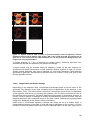
Figure 71: Optical sections with a variety of pinhole diameters (63x/1.4 objective). Pinhole
diameters from top left to bottom right: 4 AE; 2 AE; 1 AE; 0.5 AE; 0.25 AE. The strong loss of
light can be seen clearly with the small diameters, as can the pronounced background in the
images with very large diameters.
A pinhole diameter of 1 Airy is therefore the default setting. Switching objectives also
automatically adjusts the diameter of the pinhole accordingly.
A larger pinhole may be selected simply by adjusting a slider on the user interface for
specimens with weak fluorescence or high sensitivity against exposure to light. Of course,
smaller pinhole diameters may also be selected for very bright specimens. With reflecting
specimens in particular, the pinhole may be reduced to 0.2 or even 0.1 Airy units (AU) for the
thinnest possible sections.
10.2.6
Image Detail and Raster Settings
Depending on the objective used, conventional microscopes show a circular cutout of the
specimen. The diameter of the circle, multiplied by the magnification of the objective, is the
field number (FOV). The field number is therefore a microscope value which is independent
of the objective, and which, by reversing the operation, can be used to calculate the size of
the specimen being observed. A scanner always acquires square or rectangular excerpts, of
course. If such a square or rectangle is exactly circumscribed by the field of vision, than the
diagonal dimension will correspond exactly to the field number, allowing the largest possible
image to be displayed on the monitor without restrictions.
Unlike eyes or conventional cameras, scanners can simply be set to a smaller angle. A
further-enlarged section of the field of view will then be displayed on the monitor. It is thus
possible to zoom into details without the need for additional optics. As the scan angle can be
95
adjusted very quickly and continuously over a wide range, the magnification can be
increased up to around 40x simply by moving a slider. As always in microscopy, the total
magnification must be appropriate, i.e. within a suitable range, in order to obtain good
images. Other scales are important for overviews and bleaching experiments.
As errors can easily be made when interpreting scanned data, the following is an example of
how an appropriate total magnification can be calculated, as well as the information that is
automatically provided to the user by the software.
Zoom
Pan
fov 15,1
fov 21,2
Figure 72: Fields for the conventional scanner (formerly: 21.2 mm, now: 22 mm) and the
resonant scanner (15.1 mm). A smaller scanning angle increases the magnification (zoom),
while a scan offset shifts the image detail (pan) within the field of view.
The edge length of the displayed field of a conventional scanner corresponds to 15 mm
without magnification by the objective (1x scale). Field numbers of 21.2 and 22, respectively,
are thus also fully utilized (Figure 72).
That is suitable for most good research microscopes. How many elements are now actually
resolved optically in this dimension? That depends on the numerical aperture of the objective
and the wavelength. According to Ernst Abbe's formula, two points can still be distinguished
if the distance between them is not smaller than d=ë/2*NA. A line can thus contain a
maximum of 15 mm/d resolution elements (also known as "resels"). When using an actual
objective such as a plane apochromat 10x/0.4, the edge length corresponds to 1.5 mm (15
mm/10) and d=0.625 µm when using blue-green light with a wavelength of 500 nm. Such an
image would thus contain 1500/0.625=2400 optical resolution elements along each edge (x
and y direction).
Rendering this resolution in a digital pixel image would require working with twice the
resolution to prevent losses (Nyquist theorem). That would be an image with 4800 x 4800
pixels. Some purists require 3x oversampling, i.e. 7200 x 7200 pixels or 52 megapixels.
Image formats for x and y can be adjusted independently and in very fine steps, with the
Leica TCS SP5 supporting image capture sizes of up to 64 megapixels (8000 x 8000 pixels)
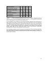
(Table 5).
Magnification
96
63
40
10
Numerical Aperture
1,4
1,25
0,4
Optical Resolution (400 nm)
μm
0,14
0,16
0,5
Intermediate Image (Edge)
mm
15
15
15
Field (Edge)
μm
238
375
1500
Resel (Field / Resolution)
1667
2344
3000
2x Oversampling
3333
4688
6000
3x Oversampling
5000
7031
9000
Table 5
Table of resolution elements at 400 nm for a variety of objectives over the
entire scan field. It becomes apparent here that a resolution of 64 megapixels (8000x8000
pixels) is appropriate for quality microscopy applications.
It is thus possible to truly capture all of the image information resolved by the microscope in a
single image at that setting. This naturally results in large data volumes, which are especially
undesirable for measurements with a high temporal resolution. Zoom is the correct solution
here. When capturing data in the standard 512 x 512 format, this means limiting the image to
a field 10 - 15 times smaller to avoid loss of information. Zoom factors of 10x and higher
provide usable data, but from rather small fields of view. The information required will
determine what constitutes an acceptable compromise here.
Such an image is initially a cutout in the center of the scan field. That is not always desirable,
as it can be difficult to center the interesting structures with such precision. However, the
scan field excerpt can be moved across the entire scan field to the actual points of interest, a
method called "panning".
97
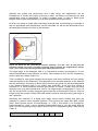
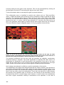
Figure 73: The same image detail in a variety of pixel resolutions. Please note that the printing
medium may not be capable of reproducing the full detail of high resolutions. You may
therefore have difficulty detecting the differences between the top two images, despite the
enormous differences in the optical resolution. This must also be taken into consideration in
publications.
The simplest solution is to combine both methods in the so-called "Zoom In" function. Simply
select a square on the monitor that encloses the structures of interest, and the instrument will
automatically select the appropriate pan and zoom values. This function is very fast and thus
easy on the specimen. An "Undo Zoom" function returns you to your starting point—for
quickly concentrating on a different cell in the field of view, for example.
The size of the grid spacing used can be found in the image properties. The spacing of the
elements in x, y and z can be found under "Voxel Size". At Zoom 1, the images calculated
above would have a grid spacing between 200 nm and 300 nm. Larger gaps would lead to a
loss of resolution when using an objective with an aperture of 0.4 (Figure 73).
Rectangular formats are important for higher image scanning rates. An additional parameter
is required here: the rotation of the scan field. As field rotation is performed optically in the
Leica TCS SP5, rotation by +/- 100º does not have any effect on the speed and possible grid
formats (Figure 74).
98
Figure 74: Zoom, Pan and Rotation combined in one example.
Finally, it must be pointed out in this section that a good microscopic image in a scientific
context must always contain a scale. Such a scale can simply be added to the image and
adjusted in its shape, color and size as required. Scales were not added to the images in this
document for the sake of clarity.
10.2.7
Signal and Noise
The gain of the capture system must be matched to the signal intensity when capturing data.
Signal strengths can vary by several orders of magnitude, making such an adjustment
necessary to ensure a good dynamic range for the scan. The goal is to distribute the full
range of intensity over the available range of grayscale values. 256 grayscale values (from 0
to 255) are available for images with 8-bit encoding. If the gain is too low, the actual signal
may only correspond to 5 grayscale values, causing the image to consist solely of those
values. If the gain is too high, parts of the signal will be truncated, i.e. they will always be
assigned the grayscale value of 255, even though differences (information) were originally
present in the signal. This image information is then lost (Figure 75).
99
Correctly setting the zero point is also important. This can be accomplished by shutting off
the illumination via the AOTF and setting the signal to zero with "Offset".
Turn the illumination back on and adjust the gain to prevent distortion.
This configuration work is simplified by special color tables such as "Glow-over/Glowunder"—a table that initially uses yellow and red for intensities in steps to indicate the signal
strengths. The grayscale value zero is always shown as green, value 255 as blue. Both
values can thus be identified immediately. The zero point is set correctly when around half
the pixels are zero—i.e. green—with the light switched off. To be safe, the offset can be set
one or two grayscale values higher to ensure that the lower signal values are not truncated.
The loss of dynamic range is negligible (approx. 0.4% per grayscale value at 8 bits).
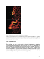
Figure 75: At the top left you see an 8-bit image (256 gray scales). At the right, the same
specimen with a considerably smaller dynamic range. Around 6 gray scales can be made out in
the false-color image at the bottom. That corresponds to less than 3 bits.
The electronic deviations from the zero point will generally be negligible; nevertheless,
occasional testing is advisable. The actual significance of adjusting the offset value is to
compensate for nonspecific or self fluorescence in the specimen at the time of the scan.
Simply set the offset value in such a manner that the background fluorescence is no longer
visible. Please note that this may also truncate signals containing image information.
Such settings must always be verified by a careful examination of the results.
The amplification of the signal must be performed after the offset correction. This operation is
quite simple with the described color table: adjust the high voltage at the PMT until no more
blue pixels are visible. We recommend focusing to ensure that the brightest signals in the
field of view are really used for the adjustment. This is also the right time to check whether
the intensity of the excitation light is correctly set. The intensity of the illumination can be
increased at the AOTF to reduce image noise. However, it must be taken into consideration
here that a higher illumination intensity is detrimental to the specimen. In the case of
100