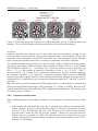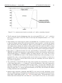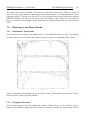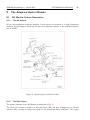
1
EUROPEAN SOUTHERN OBSERVATORY
Organisation Européene pour des Recherches Astronomiques dans l’Hémisphère Austral
Europäische Organisation für astronomische Forschung in der südlichen Hemisphäre
ESO - European Southern Observatory
Karl-Schwarzschild Str. 2, D-85748 Garching bei München
Very Large Telescope
SINFONI
User Manual
VLT-MAN-ESO-14700-3517
Version 93.2, Date 2013/12/09
Prepared
. . . . . . . . .G.
. . Hau
. . . . . . . . . . . . . . . . . . . . . . . . . . . . . . .
Date
Approved
. . . . . . . A.
. . .Kaufer
. . . . . . . . . . . . . . . . . . . . . . . . . . . . . . . .
Date
Released
Signature
Signature
. . . . . . . . C.
. . Dumas
. . . . . . . . . . . . . . . . . . . . . . . . . . . . . . . .
Date
Signature
VLT Paranal Observatory ? Telephone: +56-55-435000 ? Fax: +56-55-435001
SINFONI User Manual — Version 93.2
VLT-MAN-ESO-14700-3517
Change Record
Issue/Rev.
Date
Sect./Paragr. affected
Issue 1
Issue 1.1
01/09/2004 all
21/10/2004 12
Issue 1.2
Issue 1.3
Issue 1.4
05/01/2005
24/05/2005
12/03/2006 all parts
Issue 78.1
2006/04/24 cover & header
Issue 78.2
2006/06/07 cover & templates
Issue 78.3
2006/06/25 cover & text
Issue 79.1
2006/09/09 entire doc
Issue 79.2
2006/11/27 entire doc
Issue 80.1
Issue 80.2
2007/02/17 entire doc
2007/02/23 5 & 12
Issue 80.3
2007/05/25 all sections
Issue 80.4
2007/06/13 2.1, 2.2, 12.2.3
Issue 81.1
Issue 81.2
Issue 81.3
2007/08/26 1.3, 2.1, 5.7, 8.2.2, 12.1
2007/09/06 2.1
2007/09/10 2.1, 2.2, 8.2.2
Issue 81.4
2007/12/04 12.2
Issue 81.5
2007/12/05 12.2.2
Issue 82.1
2008/02/28 1.3, 2.2, 3.3, 7.2, 12.0
Issue 82.2
2008/05/28 5.6, 12.2
Reason/Initiation/Documents/Remarks
First release, intended for phase 1 P75
Template reference included for SV and
GTO runs in Nov 2004.
Version prepared for phase 2 of P75.
Minor changes for phase 2 of P76.
Added information on availability of
LGS and RRM modes for P78.
Issue number aligned with new format
requirements for module archivation.
IP78 phase-2 (RRM, LGS, PREimaging; also, “AutoJitterOffset” template is not offered anymore).
Small changes, mostly typos and english were corrected.
Fixed some small inconsistencies wrt
Period 79.
Fixed some small inconsistencies
throughout the text wrt grating
wavelength range.
Update for P80 (Phase 1).
Added availability of fast acquisition
template in service mode (waiver required).
Small changes for preparation of P80
(Phase 2), LGS infos updated.
Added infos about field selector orientation and offsets in auto jitter template.
Some small updates for CfP81.
Orientation of Field-Selector updated.
Updated magnitude limits of TTS for
LGS obs.
Update for P81, Phase 2; keyword
change in auto jitter template.
Corrected sign error in caption of figure related to generic offset sequence
in SKY mode.
Offering LGS without TTS (SE mode)
on a best effort basis for P82.
Explanation of PA convention and return to origin.
ii
SINFONI User Manual — Version 93.2
Issue/Rev.
Date
Sect./Paragr. affected
Issue 84
2010/01/20 1, 12.2.2; entire doc
Issue 87
2010/12/21 12, 12.3.4
Issue 88
2011/03/01 none
Issue 89
2011/08/26 2.6
Issue 90
2012/05/24 none
Issue 93
2013/09/01 All
Issue 93.1
2013/09/27 All
Issue 93.2
2013/12/09 All
VLT-MAN-ESO-14700-3517
iii
Reason/Initiation/Documents/Remarks
Update of the introduction section;
clarification (additional explanations) of
the SINFONI offset convention; general
update of the entire document.
Update for P87, Phase 2; a new template ’SINFONI ifs cal GenericOffset’ is
available, to allow efficient PSF observations in LGS-noTTS mode (Seeing
Enhancer mode).
To be used for P88; no changes w.r.t.
P87, Phase 2.
To be used for P89; details on detector
persistence added.
To be used for P90; no changes w.r.t.
P89.
To be used for P93. New section
on pupil-tracking mode added. Information in many sections are updated/revised.
To be used for P93. New figure on instrument orientation. Expanded information on Pupil Tracking mode. General tidying up.
To be used for P93 phase 2. More information on Pupil Tracking mode. Many
sections are updated.
SINFONI User Manual — Version 93.2
VLT-MAN-ESO-14700-3517
iv
SINFONI in a Nutshell
SINFONI is a near-infrared (1.1 − 2.45 µm) integral field spectrograph fed by a curvature sensing
adaptive optics module. The spectrograph operates with 4 gratings (J, H, K, H+K) providing
a spectral resolution around 2000, 3000, 4000 in J, H, K, respectively, and 1500 in H+K – each
wavelength band fitting fully on the 2048 pixels of the Hawaii 2RG (2k×2k) detector in the
dispersion direction. The SINFONI field of view on the sky is sliced into 32 slitlets. Pre-optics
allow to chose the angular size of the slices on the sky. The choices are 250 mas, 100 mas and 25
mas, leading to field of views on the sky of 8” ×8” , 3” ×3” and 0.8” ×0.8” respectively. Each
one of the 32 slitlets is imaged onto 64 pixels of the detector. Thus, one obtains 32 × 64 = 2048
spectra of the imaged region of the sky. Typical limiting magnitudes (S/N = 10 in 1h on source)
are around 17–18 mag in J, H, K.
SINFONI can be used without adaptive optics guide star, in which case the AO module just
acts as relay optics and the spatial resolution is dictated by the natural seeing. In that case,
the recommended slice width is 250 mas for a 800 ×800 field of view. The full power of the
instrument is, of course, achieved when an adaptive optics guide star is available. For best
correction, the star should be brighter than R ∼ 11 mag. However, the AO can work (and will
provide a moderate image quality improvement) with stars as faint as R ∼ 17 mag in the best
conditions. Ideally, the AO guide star should be as close as possible to the scientific target (if not
the science target itself), and usually closer than 1000 . Depending on the atmospheric conditions
(atmospheric coherence time and isoplanatic angle) the AO guide star could be chosen as far as
3000 for the AO system to still provide a mild improvement of the encircled energy.
Since Period 79, SINFONI has been operating with the Laser Guide Star (LGS). The system
provides Strehl ratio in the 10-20% range under excellent conditions. Tip-Tilt Stars (TTS) as
faint as R≤17 can be used, with a maximal separation of 1 arcmin from the science target. A new
LGS mode with no TTS (the so-called Seeing Enhancer mode, or SE mode) has been available
since Period 84. LGS requires CLEAR sky and airmass < 1.5. Please note that the LGS mode
(resp. NGS mode) so far does not support differential tracking between the Tip Tilt Star (resp.
NGS star) and the science target.
From Period 93 onwards, a new Pupil-Tracking mode is offered for the NGS mode, enabling
the use of the Spectral Angular Differential Imaging (S-ADI) technique to obtain simultaneous
imaging/spectroscopy of faint companion sources around K ≥ 5 mag sources.
SINFONI User Manual — Version 93.2
VLT-MAN-ESO-14700-3517
This page was intentionally left (almost) blank
v
SINFONI User Manual — Version 93.2
VLT-MAN-ESO-14700-3517
vi
.
.
.
.
.
1
1
1
1
2
3
Contents
1 Introduction
1.1 Scope of this document . .
1.2 Structure of this document
1.3 Latest changes . . . . . . .
1.4 Glossary . . . . . . . . . .
1.5 Abbreviations and Acronyms
I
.
.
.
.
.
.
.
.
.
.
.
.
.
.
.
.
.
.
.
.
.
.
.
.
.
.
.
.
.
.
.
.
.
.
.
.
.
.
.
.
.
.
.
.
.
.
.
.
.
.
.
.
.
.
.
.
.
.
.
.
.
.
.
.
.
.
.
.
.
.
.
.
.
.
.
.
.
.
.
.
.
.
.
.
.
.
.
.
.
.
.
.
.
.
.
.
.
.
.
.
.
.
.
.
.
.
.
.
.
.
.
.
.
.
.
.
.
.
.
.
.
.
.
.
.
.
.
.
.
.
.
.
.
.
.
.
.
.
.
.
Observing with SINFONI: from phase 1 to data reduction
2 SINFONI Performance overview
2.1 Reference source for wavefront sensing . . .
2.2 Laser Guide Star (LGS) observations . . . .
2.3 Spectrograph modes . . . . . . . . . . . . .
2.4 RRM mode . . . . . . . . . . . . . . . . . .
2.5 Pre-Imaging mode . . . . . . . . . . . . . .
2.6 Saturation and persistence limits . . . . . .
2.7 Total instrument + telescope background . .
2.8 Recommended DITs and NDITS, Object–Sky
2.9 Pupil-Tracking Mode . . . . . . . . . . . . .
2.9.1 Expected performance . . . . . . . .
2.9.2 Important considerations . . . . . . .
4
.
.
.
.
.
.
.
.
.
.
.
4
4
6
7
7
8
8
8
9
9
10
11
.
.
.
.
.
15
15
15
15
16
16
.
.
.
.
.
.
18
18
19
19
21
21
21
5 Observing with SINFONI at the VLT
5.1 Overview . . . . . . . . . . . . . . . . . . . . . . . . . . . . . . . . . . . . . . .
5.2 Visitor Mode Operations . . . . . . . . . . . . . . . . . . . . . . . . . . . . . . .
23
23
23
. . . . .
. . . . .
. . . . .
. . . . .
. . . . .
. . . . .
. . . . .
pattern
. . . . .
. . . . .
. . . . .
3 Phase 1: applying for observing time with SINFONI
3.1 Is SINFONI the right instrument for your project? .
3.1.1 The AO guide star . . . . . . . . . . . . . .
3.1.2 Limiting magnitudes . . . . . . . . . . . . .
3.2 The Exposure Time Calculator (ETC) . . . . . . . .
3.3 Proposal form . . . . . . . . . . . . . . . . . . . .
.
.
.
.
.
.
.
.
.
.
.
.
.
.
.
.
.
.
.
.
.
.
.
.
.
.
.
.
.
.
.
.
.
.
.
.
.
.
.
.
.
.
.
.
.
.
.
.
.
.
.
.
.
.
.
.
.
.
.
.
.
.
.
.
.
.
.
.
.
4 Phase 2: Preparing your SINFONI observations
4.1 Do you have all information in hand? . . . . . . . . . . . . .
4.2 SINFONI specifics to templates, OBs, and p2pp . . . . . . .
4.2.1 Templates . . . . . . . . . . . . . . . . . . . . . . .
4.2.2 Observing Blocks – OBs . . . . . . . . . . . . . . . .
4.2.3 P2PP . . . . . . . . . . . . . . . . . . . . . . . . . .
4.3 Finding Charts, README Files and OB Naming Conventions
.
.
.
.
.
.
.
.
.
.
.
.
.
.
.
.
.
.
.
.
.
.
.
.
.
.
.
.
.
.
.
.
.
.
.
.
.
.
.
.
.
.
.
.
.
.
.
.
.
.
.
.
.
.
.
.
.
.
.
.
.
.
.
.
.
.
.
.
.
.
.
.
.
.
.
.
.
.
.
.
.
.
.
.
.
.
.
.
.
.
.
.
.
.
.
.
.
.
.
.
.
.
.
.
.
.
.
.
.
.
.
.
.
.
.
.
.
.
.
.
.
.
.
.
.
.
.
.
.
.
.
.
.
.
.
.
.
.
.
.
.
.
.
.
.
.
.
.
.
.
.
.
.
.
.
.
.
.
.
.
.
.
.
.
.
.
.
.
.
.
.
.
.
.
.
.
.
.
.
.
.
.
.
.
.
.
.
.
.
.
.
.
.
.
.
.
.
.
.
.
.
.
.
.
.
.
.
.
.
.
.
.
.
.
.
.
.
.
.
.
SINFONI User Manual — Version 93.2
5.3
5.4
5.5
5.6
5.7
5.8
5.9
The influence of the Moon . . . . . .
Weather constraints . . . . . . . . .
Target Acquisition . . . . . . . . . .
Measuring the Strehl ratios, reference
Orientation convention . . . . . . . .
Offset conventions and definitions . .
Instrument and telescope overheads .
VLT-MAN-ESO-14700-3517
. . . . . .
. . . . . .
. . . . . .
PSF stars
. . . . . .
. . . . . .
. . . . . .
.
.
.
.
.
.
.
.
.
.
.
.
.
.
.
.
.
.
.
.
.
.
.
.
.
.
.
.
.
.
.
.
.
.
.
.
.
.
.
.
.
.
.
.
.
.
.
.
.
.
.
.
.
.
.
.
6 The SINFONI data reduction pipeline
6.1 Required Input Frames for the Pipeline . . . . . . . . . . . . .
6.1.1 Reference Files . . . . . . . . . . . . . . . . . . . . . .
6.1.2 Raw frames . . . . . . . . . . . . . . . . . . . . . . .
6.1.3 Calibration Products . . . . . . . . . . . . . . . . . . .
6.2 Data Reduction Steps . . . . . . . . . . . . . . . . . . . . . .
6.2.1 Detector Linearity and Bad Pixel Mask Determination .
6.2.2 Bad Pixel mask and Master Dark Determination . . . .
6.2.3 Master Spatial Flat and bad pixel determination . . . .
6.2.4 Detector’s distortion and slitlet distances determination
6.2.5 Wavelength solution determination . . . . . . . . . . .
6.2.6 Standard star data reduction . . . . . . . . . . . . . .
6.2.7 PSF data reduction . . . . . . . . . . . . . . . . . . .
6.2.8 Science observations . . . . . . . . . . . . . . . . . . .
II
.
.
.
.
.
.
.
.
.
.
.
.
.
.
.
.
.
.
.
.
.
.
.
.
.
.
.
.
.
.
.
.
.
.
.
.
.
.
.
.
.
.
.
.
.
.
.
.
.
.
.
.
.
.
.
.
.
.
.
.
.
.
.
.
.
.
.
.
.
.
.
.
.
.
.
.
.
.
.
.
.
.
.
.
.
.
.
.
.
.
.
.
.
.
.
.
.
.
.
.
.
.
.
.
.
.
.
.
.
.
.
.
.
.
.
.
.
.
.
.
.
.
.
.
.
.
.
.
.
.
.
.
.
.
.
.
.
.
.
.
.
.
.
.
.
.
.
.
.
.
.
.
.
.
.
.
.
.
.
.
.
.
.
.
.
.
.
.
.
.
.
.
.
.
.
.
.
.
.
.
vii
.
.
.
.
.
.
.
23
24
24
25
26
26
27
.
.
.
.
.
.
.
.
.
.
.
.
.
28
28
28
28
29
30
30
30
31
31
31
32
32
32
SINFONI: a detailed description of the instrument
7 General description
7.1 Observing with Adaptive Optics . . . . .
7.1.1 Atmospheric turbulence . . . . .
7.1.2 Adaptive Optics . . . . . . . . .
7.2 The Laser Guide Star mode . . . . . . .
7.2.1 Background information on LGS .
7.2.2 LGS mode at Paranal-UT4 . . .
7.3 Observing in the Near-Infrared . . . . . .
7.3.1 Atmospheric Transmission . . . .
7.3.2 Background Emission . . . . . .
7.3.3 Spectrophotometric Calibration .
7.4 Integral Field Spectroscopy . . . . . . .
33
.
.
.
.
.
.
.
.
.
.
.
33
33
33
33
35
35
35
36
36
36
37
38
8 The Adaptive-Optics Module
8.1 AO-Module System Description . . . . . . . . . . . . . . . . . . . . . . . . . . .
8.1.1 The AO Adapter . . . . . . . . . . . . . . . . . . . . . . . . . . . . . . .
40
40
40
.
.
.
.
.
.
.
.
.
.
.
.
.
.
.
.
.
.
.
.
.
.
.
.
.
.
.
.
.
.
.
.
.
.
.
.
.
.
.
.
.
.
.
.
.
.
.
.
.
.
.
.
.
.
.
.
.
.
.
.
.
.
.
.
.
.
.
.
.
.
.
.
.
.
.
.
.
.
.
.
.
.
.
.
.
.
.
.
.
.
.
.
.
.
.
.
.
.
.
.
.
.
.
.
.
.
.
.
.
.
.
.
.
.
.
.
.
.
.
.
.
.
.
.
.
.
.
.
.
.
.
.
.
.
.
.
.
.
.
.
.
.
.
.
.
.
.
.
.
.
.
.
.
.
.
.
.
.
.
.
.
.
.
.
.
.
.
.
.
.
.
.
.
.
.
.
.
.
.
.
.
.
.
.
.
.
.
.
.
.
.
.
.
.
.
.
.
.
.
.
.
.
.
.
.
.
.
.
.
.
.
.
.
.
.
.
.
.
.
.
.
.
.
.
.
.
.
.
.
.
.
SINFONI User Manual — Version 93.2
8.2
9 The
9.1
9.2
9.3
9.4
9.5
9.6
9.7
8.1.2 The Main Optics . . . . .
8.1.3 The Corrective Optics . .
8.1.4 The Wavefront Sensor . .
8.1.5 LGS mode elements . . .
8.1.6 Calibration Unit . . . . .
AO-module System Performances
8.2.1 NGS performances . . . .
8.2.2 LGS performances . . . .
VLT-MAN-ESO-14700-3517
.
.
.
.
.
.
.
.
.
.
.
.
.
.
.
.
integral field spectrograph SPIFFI
Pre-optics . . . . . . . . . . . . . .
Image slicer . . . . . . . . . . . . .
Spectrometer collimator . . . . . . .
Grating wheel . . . . . . . . . . . .
Spectrometer camera . . . . . . . .
Sky-spider . . . . . . . . . . . . . .
Detector characteristics . . . . . . .
.
.
.
.
.
.
.
.
.
.
.
.
.
.
.
.
.
.
.
.
.
.
.
.
.
.
.
.
.
.
.
.
.
.
.
.
.
.
.
.
.
.
.
.
.
.
.
.
.
.
.
.
.
.
.
.
.
.
.
.
.
.
.
.
.
.
.
.
.
.
.
.
.
.
.
.
.
.
.
.
.
.
.
.
.
.
.
.
.
.
.
.
.
.
.
.
.
.
.
.
.
.
.
.
.
.
.
.
.
.
.
.
.
.
.
.
.
.
.
.
.
.
.
.
.
.
.
.
.
.
.
.
.
.
.
.
.
.
.
.
.
.
.
.
.
.
.
.
.
.
.
.
.
.
.
.
.
.
.
.
.
.
.
.
.
.
.
.
.
.
.
.
.
.
.
.
.
.
.
.
.
.
.
.
.
.
.
.
.
.
.
.
.
.
.
.
.
.
.
.
.
.
.
.
.
.
.
.
.
.
.
.
.
.
.
.
.
.
.
.
.
.
.
.
.
.
.
.
.
.
.
.
.
.
.
.
.
.
.
.
.
.
.
.
.
.
.
.
.
.
.
.
.
.
.
.
.
.
.
.
.
.
.
.
.
.
.
.
.
.
.
.
.
.
.
.
.
.
.
.
.
.
.
.
.
.
.
.
.
.
.
.
.
.
.
.
.
.
.
.
.
.
.
.
.
.
.
.
.
.
.
.
.
.
.
.
.
.
.
.
.
.
.
.
.
.
.
.
.
.
.
.
.
.
.
.
.
.
.
.
.
.
.
.
.
viii
.
.
.
.
.
.
.
.
40
41
42
43
45
46
46
47
.
.
.
.
.
.
.
49
49
49
49
50
51
51
52
10 Software Overview
53
III
55
Reference Material
11 The SINFONI science calibration plan
11.1 The science calibrations in a nutshell . . . . . . . . . . . . . . . . . . . . . . . .
55
55
12 SINFONI template reference
12.1 Acquisition Templates . . . . . . . . . .
12.1.1 SINFONI ifs acq NGS . . . . . .
12.1.2 SINFONI ifs acq NGSfast . . . .
12.1.3 LGS acquisition template . . . .
12.1.4 SINFONI ifs acq noAO . . . . .
12.1.5 RRM acquisition templates . . .
12.2 Science Templates . . . . . . . . . . . .
12.2.1 SINFONI ifs obs FixedSkyOffset .
12.2.2 SINFONI ifs obs GenericOffset .
12.2.3 SINFONI ifs obs AutoJitter . . .
12.2.4 SINFONI ifs obs AutoJitterSpider
12.3 Nighttime Calibration Templates . . . .
12.3.1 SINFONI ifs cal StandardStar . .
12.3.2 SINFONI ifs cal PSF . . . . . . .
12.3.3 SINFONI ifs cal NGS . . . . . .
12.3.4 SINFONI ifs cal GenericOffset . .
56
58
60
62
63
64
65
65
66
67
69
70
71
71
72
72
73
.
.
.
.
.
.
.
.
.
.
.
.
.
.
.
.
.
.
.
.
.
.
.
.
.
.
.
.
.
.
.
.
.
.
.
.
.
.
.
.
.
.
.
.
.
.
.
.
.
.
.
.
.
.
.
.
.
.
.
.
.
.
.
.
.
.
.
.
.
.
.
.
.
.
.
.
.
.
.
.
.
.
.
.
.
.
.
.
.
.
.
.
.
.
.
.
.
.
.
.
.
.
.
.
.
.
.
.
.
.
.
.
.
.
.
.
.
.
.
.
.
.
.
.
.
.
.
.
.
.
.
.
.
.
.
.
.
.
.
.
.
.
.
.
.
.
.
.
.
.
.
.
.
.
.
.
.
.
.
.
.
.
.
.
.
.
.
.
.
.
.
.
.
.
.
.
.
.
.
.
.
.
.
.
.
.
.
.
.
.
.
.
.
.
.
.
.
.
.
.
.
.
.
.
.
.
.
.
.
.
.
.
.
.
.
.
.
.
.
.
.
.
.
.
.
.
.
.
.
.
.
.
.
.
.
.
.
.
.
.
.
.
.
.
.
.
.
.
.
.
.
.
.
.
.
.
.
.
.
.
.
.
.
.
.
.
.
.
.
.
.
.
.
.
.
.
.
.
.
.
.
.
.
.
.
.
.
.
.
.
.
.
.
.
.
.
.
.
.
.
.
.
.
.
.
.
.
.
.
.
.
.
.
.
.
.
.
.
.
.
.
.
.
.
.
.
.
.
.
.
.
.
.
.
.
.
.
.
.
.
.
.
.
.
.
.
.
.
.
.
.
.
SINFONI User Manual — Version 93.2
VLT-MAN-ESO-14700-3517
12.3.5 SINFONI ifs cal ArcsAtt . . . . . . . . . . . . . . . . . . . . . . . . . . .
12.3.6 SINFONI ifs cal LampFlatsAtt . . . . . . . . . . . . . . . . . . . . . . . .
12.4 Daytime Calibration Templates . . . . . . . . . . . . . . . . . . . . . . . . . . .
13 The Spectral Resolution of SINFONI
ix
74
74
75
77
SINFONI User Manual — Version 93.2
1
1.1
VLT-MAN-ESO-14700-3517
1
Introduction
Scope of this document
The SINFONI User Manual provides comprehensive information about the technical characteristics
of the instrument, the observations procedures and the reduction of SINFONI data. The actual
version was updated with the latest information about the detector and observing modes offered.
We welcome any comments and suggestions, which should be addressed to our User Support Department – [email protected] .
In addition to this User Manual, (complementary) information about SINFONI is also provided
on the SINFONI webpage ( http://www.eso.org/sci/facilities/paranal/instruments/
sinfoni/ ) which you are invited to visit regularly for any last-minute update.
1.2
Structure of this document
The document is structured in 3 parts. Part 1 (I) takes you step by step through the essentials
(writing your proposal in phase 1, preparing your observations in phase 2, conducting your observations at the telescope and reducing your data). If you want to learn more about the instrument
itself, you might want to read through Part 2 (II). Finally, Part 3 (III) contains the SINFONI
calibration plan, a description of the templates and collected useful reference material.
1.3
Latest changes
- From P93 onwards, SINFONI will be offering a new Pupil-Tracking mode allowing medium contrast imaging/spectroscopy of companions around K ≥ 5 mag sources.
- Since P92, SINFONI has been operating with the new solid-state laser PARLA with on-sky power
of ∼ 7 W. PARLA is available to SINFONI every night.
- Since P84, SINFONI has been offered with a new LGS mode named ”Seeing-Enhancer” (SE)
mode which will not require a TTS – only the high-orders of aberration are corrected, but no tiptilt. The SE mode provides some improvement with respect to the seeing-limited (no-AO) mode,
but only under very good conditions. Therefore, the SE mode requires seeing constraints of 0.8”
or better.
- Since P81, the use of the fast acquisition template is offered in service mode, but a waiver needs
to be submitted to the User Support Department at the time of preparation of the Phase 2 OBs
(see http://www.eso.org/sci/observing/phase2/SMGuidelines.html for additional information).
- Since P78, Paranal’s Rapid Response Mode (RRM) is offered for SINFONI too (please see http:
//www.eso.org/sci/observing/phase2/RRMObservation.html for more information about
the RRM mode). The Rapid Response Mode is offered for observations of transient phenomena
such as gamma-ray bursts or supernovae in semi-automatic mode. The user (PI or Co-I of an
approved target-of-opportunity program) submits an ftp file with the coordinates of the target to
SINFONI User Manual — Version 93.2
VLT-MAN-ESO-14700-3517
2
a specific ftp server on Paranal. A special program at the telescope continuously monitors this ftp
directory. When it detects a file, it checks if the filename corresponds to an approved activation
code. If this is the case and if the required instrument is currently used at the telescope, the
on-going observations are ended and a new BOB starts an OB with the same name as the ftp file.
The telescope automatically presets to the coordinates specified in the ftp file, and the requested
observations are performed straight away. PIs of approved SINFONI ToO programs requesting this
mode need to prepare their OBs in the usual way. However, these RRM programs use specific
acquisition templates described in the template section of this manual (12).
- Although commissioning activities occurred until 2008, the Laser Guide Star (LGS) facility has
been offered to SINFONI users as early as P79 (mostly in service mode). This mode provides
significant improvement for programs which were limited to the no-AO mode, due to the lack of an
adequate natural guide star for the AO system. Please note, nevertheless, that LGS observations
can only be done under clear sky conditions and still require the use of a Tip-Tilt Star (TTS) to
reach optimal correction. Moreover the airmass must be less than 1.5. At the time being, Strehl
improvement up to ∼20% have been measured under the best seeing conditions. TTS with R≤17
have been successfully used with separations from the science target as large as ∼1 arcmin. LGS
can only be used for programs having specifically requested this mode in the Phase 1 proposal, and
after approval given by the OPC.
1.4
Glossary
Active optics: This is the active control of the primary and secondary mirrors of the telescope.
It is performed using a telescope guide star.
Adaptive optics: This is the correction of wavefront errors induced by atmospheric turbulence.
The wavefront is measured from a guide star (either NGS or LGS, see below) and the corrections
are sent to the deformable mirror within the instrument. Although the instrument can run in closed
loop without the active optics system controlling the primary and secondary mirrors, one gets better
adaptive optics performance if the active optics system of the telescope is running.
Laser Guide Star, LGS: The artificial star created by the sodium laser at an altitude of ∼90 km.
Natural Guide Star, NGS: The astronomical object used to close the AO loop. It is usually
a star, but it can also be an extended object as long as it provides sufficient contrast (at visible
wavelengths) and fits within the wavefront sensor field of view (∼2.5 arcsec).
Pupil-tracking: Instead of Field-Tracking, where the sky orientation is kept fixed during an exposure, in Pupil-Tracking mode the pupil of the telescope (hence the diffraction spikes) is fixed with
respect to the detector, while the sky rotates.
Tip-Tilt Star, TTS: The star used in LGS mode to sense and correct tip-tilt aberrations.
SINFONI User Manual — Version 93.2
1.5
VLT-MAN-ESO-14700-3517
Abbreviations and Acronyms
ADI
AO
APD
DM
DMD
ESO
ETC
FC
FoV
FWHM
LGS
MPE
NACO
NGS
NIR
NOVA
OB
P2PP
PSF
QC
RRM
RTC
S-ADI
SINFONI
SPAXEL
SM
SR
TIO
TTS
USG
VLT
VM
WF
WFS
Angular Differential Imaging
Adaptive Optics
Avalanche Photo-Diode
Deformable Mirror
Data Management Division
European Southern Observatory
Exposure Time Calculator
Finding Chart
Field of View
Full Width at Half Maximum
Laser Guide Star
Max-Planck Institut für Extraterrestrische Physik
NAOS–CONICA or Nasmyth AO System–COude Near-Infrared CAmera
Natural Guide Star
Near InfraRed
Nederlandse Onderzoekschool Voor Astronomie
Observing Block
Phase II Proposal Preparation
Point Spread Function
Quality Control
Rapid Response Mode
Real Time Computer
Spectroscopic Angular Differential Imaging
Spectrograph for INtegral Field Observations in the Near Infrared
Spatial (resolution) Elements on the sky
Service Mode
Strehl Ratio
Telescope and Instrument Operator
Tip-Tilt Star
User Support Group
Very Large Telescope
Visitor Mode
Wave Front
Wave Front Sensor
3
4
Part I
Observing with SINFONI: from phase 1
to data reduction
2
SINFONI Performance overview
The following section gives a brief overview of the SINFONI performances. We will present more
information in Section 8.2 and we refer to the Exposure Time Calculator (ETC) which should be
used to estimate the feasibillity of your science observations. The SINFONI ETC can be found at
http://www.eso.org/observing/etc/.
2.1
Reference source for wavefront sensing
For SINFONI (NGS or LGS), the curvature wavefront sensing occurs at optical wavelengths (<1µm)
with avalanche photo diodes (APDs), which show a high photon response over a very broad
wavelength range.
A natural AO guide star (NGS) should ideally be bright, close and compact. We will present in this
section a brief overview on what can be done with the available AO guide star for the user selected
science targets.
Please note that there is no perfect correlation between seeing, NGS parameters (brightness, distance, . . . ) and the Strehl ratio of the obtained data. The coherence times and isoplanatic angles
may be distributed over a relatively wide range for a given atmospheric optical seeing value (FWHM)
and spectral range (J, H or K).
The distance of the AO guide star: Two identical field selectors, FS, (one for NGS, the other
for LGS) allow to pick the AO guide star within a ∼ 20 ×10 field centered on the spectrograph field.
Note that the vertical axis of the FS field of view is rotated by ∼25 deg., i.e. the Y-axis
is positioned ∼25 deg. clockwise from East (see Fig. 1). A check has been introduced
in P2PP to inform the user in case the selected reference star is located outside the
range of the FS, or if the sequence of offsets bring the FS beyond its mechanical limit.
However, it is important to note that the AO performance will strongly degrade for AO guide stars
at distances greater than 10 to 15 seconds depending on the selected wavelength band (J, H or
K). Under excellent conditions, bright stars as far as 2000 –3000 can still be used to provide a mild
improvement of the image quality.
The brightness of the AO guide star: The intra- and extra-focal pupil of the AO guide star is
imaged on a lenslet array, and each lenslet fed to an Avalanche Photo Diode (APD) that ultimately
forwards its signal to the Real Time Computer (RTC).
The flux on the APD is limited to 1 million counts (in order not to damage the devices) and thus,
stars brighter than R∼11 mag are dimmed by a set of neutral density filters (for up to ∼ 9 mag).
Hence, stars brighter than R∼2 mag cannot be used as AO guide star. Stars brighter than R∼11
mag will not improve further the performance of the AO system. Note also the detector persistence
SINFONI User Manual — Version 93.2
VLT-MAN-ESO-14700-3517
5
Figure 1: Orientation and size of the Field Selector field-of-view.
limit of SPIFFI effectively limits the source magnitude to K ≥ 6 – 7 mag if the AO guide star is
also the science target.
Good correction under average seeing is still obtained with stars as faint as R∼14 mag. Any fainter
guide star will then require very good or excellent atmospheric conditions to obtain diffraction
limited images. Partial correction maybe obtained down to R ∼ 17 magnitudes.
In Service mode: AO observations with AO guide stars much fainter than R∼14 mag will require
excellent observing conditions. The feasibility of such a project must be carefully evaluated and the
derived observing constraints should be well selected in the proposal as well as in the later phase
of observation preparation.
In Visitor mode: the above recommendation for service mode projects is also valid in visitor
mode. In cases in which there is only a faint AO guide star, one would, in parallel, prepare
observations for no AO, seeing limited observations. These backup projects for periods in which the
AO loop cannot be closed on faint target should be authorized well in advance to the observation
run, unless the science objectives as given in the proposal can be reached with seeing limited
observations as well.
The color of the AO guide star The color of the guide star is important for two reasons:
• The very broad response curve of the APDs extends from 450nm to 900nm with the peak
SINFONI User Manual — Version 93.2
VLT-MAN-ESO-14700-3517
6
response around 650nm. Thus, the R band magnitude provides only a crude estimate of the
number of photons detected by the Wave-Front Sensor (WFS). For M-stars and later spectral
types as well as for other very red objects (B-R > 2.2) there will be less light detected by
the APDs than for a guide star with a flat spectrum of the same magnitude.
• The color is also essential for atmospheric refraction compensation. The WFS corrects
the telescope guiding for the atmospheric refraction difference between its (optical) guiding
wavelength and the (near-infrared) central wavelength of the spectrograph set-up. Once the
response curve of the WFS is taken into account, the optical guiding wavelength can be
derived from the (B-R) color as follows:
Guiding wavelength(nm)= 590 + 40∗(B-R)
The observation software will take care of the guiding wavelength once the color is entered
into the observation templates.
2.2
Laser Guide Star (LGS) observations
This section provides the necessary information for Phase I preparation using LGS. Additional information may be provided on the SINFONI website ( http://www.eso.org/sci/facilities/
paranal/instruments/sinfoni/ ) to which you are encouraged to check. Please note that
LGS observations can only be carried out under clear (CLR) or photometric (PHO)
observing conditions, at airmass < 1.5. Thus objects with declinations south of ∼ −70
degrees and north of ∼ +20 degrees cannot be observed.
In normal LGS mode, a Tip-Tilt Star (TTS) is required for tip-tilt measurements of the wavefront.
The TTS needs to be located within a strict maximum distance of 1 arcmin from the science target
(the field accessible to the Strap Field Selector is 1’x2’, see previous section for a description of
the field selector orientation). The TTS should also be brighter than R = 17 mag, ideally in the
range R = 12–13.5 mag. Note that the correction will be strongly degraded with increasing distance
of the TTS from the science target, and with decreasing brightness of the TTS. By comparison
with the case of an on-axis NGS star, under median seeing conditions for Paranal, the achieved
Strehl ratio will be degraded by a factor of two for a TTS that is 40” from the science target. It
is also important to remember that due to the Cone Effect, the maximum Strehl achievable with
the LGS is significantly less than the one obtained with a bright NGS. The SINFONI ETC includes
observations with the LGS mode (see http://www.eso.org/observing/etc/). One can expect
the laser to create an artificial star whose magnitude will be V = 12–13 mag.
The TTS must be a single star and not a binary; there should not be a star with similar
brightness within 300 distance; failure to do so will likely cause a failure in the AO loop. The user
should advice in the README if crowding can be a problem for the TTS.
LGS observations are only possible for airmass < 1.5. Users should set the maximum airmass
in their OBs to < 1.5.
In summary, you must make sure that you have a TTS within a distance of 1 arcmin (maximum)
from your science target, which must be a single star. You should clearly state why you need to
use this mode, and include the characteristics of the TTS (V or R band magnitude, RA, DEC, and
spectral type if known). LGS observations can only be carried out under clear sky conditions (no
cirrus or any type of clouds).
SINFONI User Manual — Version 93.2
VLT-MAN-ESO-14700-3517
7
Starting officially with P84, SINFONI also offers a new LGS mode not requiring the use of a TTS
(no tip-tilt correction), the so-called Seeing-Enhancer (SE) mode. Nevertheless, in addition to
specifying CLR or better for the sky transparency, users requesting the SE mode must specify a
seeing better than 0.8” in their phase I application. For highly challenging LGS observations (e.g.
faint TTS and/or large TTS distances), you should consider using the SE mode instead of the full
LGS mode. To improve the chances of your OB being successfully executed, you may also want to
specify in the README in your Phase 2 materials to ask to automatically fall-back to SE mode if
a full LGS mode fails.
2.3
Spectrograph modes
Field of view The pre-optics of the spectrograph allow to chose between 3 plate-scales, providing
fields of 800 ×800 , 300 ×300 , 0.800 ×0.800 . Each of these fields is then cut into 32 slices, and each
slice is projected onto 64 detector pixels. Thus, the spatial resolution elements (spaxels) on the
sky are rectangular.
Field of view
800 ×800
300 ×300
0.800 ×0.800
Spaxel size on the sky
125mas×250mas
50mas×100mas
12.5mas×25mas
Wavelength bands Four gratings are installed on a turret in the spectrograph: J,H,K, H+K.
The dispersions are chosen such that the full wavelength range is covered by the detector in each
case.
Band
J
H
K
H+K
Dispersion
0.15nm/pix
0.20nm/pix
0.25nm/pix
0.50nm/pix
FWHM of line
∼4pix
∼3pix
∼2pix
∼2pix
Resolution
∼2000
∼3000
∼4000
∼1500
lambda range
1.10 – 1.40 µm
1.45 – 1.85 µm
1.95 – 2.45 µm
1.45 – 2.45 µm
The characterization is complicated by the fact that the spectral PSF is different in each platescale, i.e. the FWHM of the spectral features (i.e. the spectral resolution) varies as a function of
plate scale. See part III for details.
2.4
RRM mode
Rapid Response Mode observations with SINFONI are offered since P78. Both NGS and noAO modes are possible, although we expect most of the programs will not have a sufficiently
bright nearby object to be used as NGS for the AO system. If AO can be used in NGS mode,
please refer to the information available in section 2.1 to understand the limitations imposed
by this mode. General informations about Paranal’s RRM observations are available at http:
//www.eso.org/sci/observing/phase2/RRMObservation.html .
SINFONI User Manual — Version 93.2
2.5
VLT-MAN-ESO-14700-3517
8
Pre-Imaging mode
In case of any uncertainty concerning the feasibility of a program (e.g., source brightness, or Strehl
achieved for a faint NGS star), you can request a pre-imaging run to obtain a small subset of data.
Such dedicated pre-imaging run must be explicitly requested in the Phase 1 proposal.
2.6
Saturation and persistence limits
In open loop noAO observations the target should not be brighter than 5th magnitudes in J, H
and K and 6th magnitude in H+K. In closed loop NGS observations neither the target nor the
natural guide star must be brighter than these magnitudes (unless the fast acquisition template is
used, in which case the limits are brighter by 1 and 2 magnitudes for the 0.1”/pix and 0.025”/pix
scales respectively). These limits are set to avoid saturation during the acquisition which is by
default taken with the widest 800 ×800 scale. In visitor mode the acquisition on the widest scale
may be avoided with the template SINFONI ifs acq NGS. This will however require excellent coordinates and additional precaution at the end of the observation when presetting to the next target.
Note: The detector can show a strong persistence effect, even after being illuminated below
the saturation level (typically ∼10 000 ADUs). To exclude any risk of artefacts produced by
wavelength-dependent detector persistence, DITs must be selected such that fluxes are at most
8000 ADUs/DIT/pixel for K, 7000 ADUs/DIT/pixel for H and H+K, and 6000 ADUs/DIT/pixel
for J throughout the spectral range covered. Please note that if illumination was close or beyond
saturation, the time scale to recover from the persistence is longer than an observing night; in fact,
as shown in Fig. 2, after such a worst case saturation event persistence artefacts can last up to
several days and severely affect subsequent observations (both science and calibrations) !
2.7
Total instrument + telescope background
The total instrument + telescope background was measured in the 250 mas plate scale, as flux
per pixel (250 mas × 125 mas) for the two cases “no OH avoidance” (i.e., averaging over the full
spectral range) and “with OH avoidance” (i.e., avoiding the brightest OH lines).
Band
J
H
K
H+K
incl. OH
0.14
1.26
3.64
5.96
between OH
0.07 e− /s
0.11 e− /s
0.90 e− /s
0.80 e− /s
This converts to the following magnitude per square arcseconds:
Band
J
H
K
H+K
incl. OH
15.9
13.9
12.6
13.2
between OH
16.7 mag
16.5 mag
14.2 mag
15.3 mag
SINFONI User Manual — Version 93.2
VLT-MAN-ESO-14700-3517
9
Figure 2: Decay of persistence artefacts after a worst case saturation event, demonstrating that
such artefacts can last up to several days and severely affect subsequent observations (both science
and calibrations). In the shown example, the persistence was revealed and traced through the flux
ratio of slitlets 17 and 32 in dark exposures of DIT = 600 s.
2.8
Recommended DITs and NDITS, Object–Sky pattern
For long exposures on faint targets in which no saturation risk is given, we recommend to work
with NDIT = 1, and a DIT depending on the frequency with which the sky should be obtained.
For exposure times longer than 150 s it is mandatory in service mode to select the DIT from the
recommended values of 150 s, 300 s, 600 s or 900 s.
For short exposures we recommend DIT values of 0.83 s, 1 s, 2 s, 5 s, 10 s, 15 s, 20 s, 30 s, 60 s or
100 s to reduce the calibration load and to share the calibration data with other projects.
The standard templates support an ABBA pattern, that is Object and Sky frames are alternated
with 50% of the total time spent on the object. Observation sequences with Object–Sky patterns
in which less time would be spent on the sky is commonly used, when bright objects are observed.
For a source fairly isolated and significantly smaller than the used SINFONI field of view (e.g., a
source significantly smaller than 800 × 800 ), there exists the possibility to obtain the sky background
measurements within the field of view by applying offsets to place the target successively into the
four ‘quadrants’ of the detector while simultaneously monitoring the sky background in the other
three (in the ideal case entirely empty) ‘quadrants’.
2.9
Pupil-Tracking Mode
From P93 onwards, a mode – Pupil-Traking – will be offered, allowing the S-ADI (Spectrocopic
ADI) technique to obtain spectra/images of faint companions.
SINFONI User Manual — Version 93.2
VLT-MAN-ESO-14700-3517
10
Figure 3: PSF drift over the course of 1.3 hours as a function of position in the FOV, in units of
0.012500 .
2.9.1
Expected performance
Early performance estimation is based on pupil-tracking observations of a K = 7.8 mag B9V star
(with no companion), with artificial companion signals injected into the data, and then analysed
using standard 2-D ADI reduction techniques. The observations were centred around meridian
transit, with a total elapsed time of 1.3 hours (including acquisition), and a total field rotation of
57o , and airmass of ∼ 1.0. The observations were done with the 25 mas scale and K band. The
ambient conditions were good, with 2.8ms coherence time and a guide star FWHM of 0.500 on the
guide probe (in the visible). A DIT of 25s was used, keeping the mean counts to ∼ 8000 ADUs
for the central spaxel. The time between DITs (i.e. readout time) was 20s.
The data was reduced using the SINFONI pipeline, with the parameters chosen such that the
individual data cubes were made from each exposure (rather than all combined into one cube).
These are then spatially over-sampled into 256 × 256 × 2218 pixel cubes, from which we extracted
4 sub cubes outside the main telluric absorption bands (at 2.03–2.04 µm, 2.10–2.12 µm, 2.38–2.41
µm and 2.10–2.42 µm). Afterwards, 2-D gaussian PSFs were fitted to measure the PSF x and y
positions as a function of time, shown in Fig. 3. This shows that the drift over 1.3 hours was 0.02500
, roughly the same order of magnitude as the precision for the flexure compensation. Hereafter,
the results are reported for the first sub-cube (2.03–2.04 µm); the findings with the other cubes
SINFONI User Manual — Version 93.2
VLT-MAN-ESO-14700-3517
11
Figure 4: Recovered images after injection of artificial secondary sources of different fluxes and
distances. The red circles indicate the expected positions of the artificial secondaries.
are similar.
Artificial secondaries were injected into the data, which was then processed by filtering out the
hot pixels and the primary spectral energy (using a high-pass filter). An anisotropic PSF was also
convolved. After recentering, a master PSF was made, and it was subtracted off the individual
cubes. Finally the individual frames were re-rotated, re-normalised and median combined.
The artificial secondary was injected into the data covering a range of distances from the primary,
with varying polar angles. Different fluxes for the secondary were tested: 100, 10, 1 and 0.5 AUDs,
with the primary peak flux at ∼ 1300 ADUs. Fig. 4 shows the results of the processed data. At
∆mK = 7.8, it is still possible to detect the secondary at about 3 – 6 λ/D (0.1700 – 0.2900 )
from the primary. Fig. 5 shows the 5-σ theoretical contrast curve (without secondary injection)
as a function of distance (λ/D), while Fig. 6 shows the expected 5-sigma contrast of SINFONI
compared with other example contrast curves, showing that medium contrasts between 6 and 8.5
magnitudes (at 5-σ significance) can be expected at distances between 0.1700 and 0.2900 for the 25
mas scale.
Note that the above utilised standard 2-D ADI techniques but it is also possible to combine this
with Spectroscopic Differential Imaging (SDI) techniques (e.g. Thatte et al 2007), where the PSF
is obtained and subtracted off by scaling the PSF of adjacent wavelength slices. Thus further gains
in sensitivity may be possible.
2.9.2
Important considerations
Before deciding whether Pupil-tracking is suitable for your program, the following must be considered:
• Pupil-tracking will work with NGS mode only. It can work with all filters and grating combinations. However, at time of writing (December 2013) we have only tested the 25 mas scale
(0.8”x0.8” FOV). The 100 mas (3.2”x3.2”) and 250 mas (8”x8”) scales remain untested,
but with these 2 scales the PSF will be under sampled. Therefore for most situations the
250mas scale is not suitable for S-ADI. The 100 mas scale may be usable but one could
consider making sub-pixel offsets between exposures to have some sampling of the PSF (or
perhaps it is unnecessary).
SINFONI User Manual — Version 93.2
VLT-MAN-ESO-14700-3517
12
Figure 5: 5-σ contrast curve based on sub-cube # 1, with no secondary injected.
• The 25 mass scale has the disadvantage that, due to the small FOV (0.8” ×0.8” ), with the
star is put at the centre of the FOV, then one can only find companions about < 0.3” from
the primary.
• Pupil-tracking only works with the primary star on-axis only. In particular, there is no way
to place the primary off the FOV and have the field to rotate around it – the field will always
rotate around the axis of the instrument. Hence it is not possible to observe companions of
very bright stars by placing the primary off the field-of-view and expect the field to rotate
around it. Small offsets from the centre of the FOV is possible, but the primary’s position will
drift with time due to the field rotation, which must be corrected for during data-reduction.
• Note there is a difference between the way pupil-tracking is implemented in NACO and
SINFONI. For NACO the instrument is automatically rotated in an orientation such that the
telescope M2 spiders (i.e. diffraction spikes) are always aligned to the x and y axes of the
detector. For SINFONI the rotator of the instrument simply stops (after presetting to a user
specified PA on sky), so the telescope spiders can be fixed at any orientation. It gives more
flexibility for the user to choose where best to place the secondary, but at the expense of
more work in preparation.
• The combination of small FOV and the large pixels (spaxels) also means that you will need
a fairly large field rotation (> 30 degrees) to avoid self-subtraction. Note also because the
spaxels of SINFONI are rectangular (twice as tall as wide), one gets more sampling if the
secondary is placed near 12 or 6 o’clock on the FOV. Keeping the secondary moving mainly
along an image slice (i.e. moving mainly horizontally on the FOV) also minimise the effects
of image distortion and reconstruction.
• Another major restriction (compared with NACO) is the need to avoid persistence on the
detector; which means one should keep the maximum count in the spectral continuum below
about 6000 – 8000 AUDs per DIT; see § 2.6 for the actual limits. This means that, for the
25mas scale and minimum DIT, the limits for J, H, K and H+K are 5.0, 5.0, 4.4 and 6.0
SINFONI User Manual — Version 93.2
VLT-MAN-ESO-14700-3517
13
Figure 6: Expected contrasts from SINFONI (blue shaded region) compared to example contrast
curves from the International Deep Planet Survey (Galicher et al 2012).
mag respectively (note that these are quoted for guidelines only; you should use the Exposure
Time Calculator to check the actual peak counts).
• Given the minimum DIT is 0.83 seconds and frames are read out individually (i.e. no cube
mode), much care must be made in the target selection. There is no coronograph on
SINFONI, and persistence must be avoided since in the worst case it can last for many
days, ruining the observations of the other observers. Ideally one should ask in the README
for the observations to be done at the end of the night to minimise the possibility of other
people’s observations being affected by any persistence effects.
• To minimise overheads and maximise the S/N , and to avoid smearing out too much the
signal for a fast rotator, one would usually limit the readout to be about once every 1 to 2
minutes. However, the current overheads are rather large for short DITs, with an efficiency
of ∼ 35% – 60%. For example, with DIT = 3, and N DIT = 15, the total duty cycle time
is ∼ 125 seconds, yielding a 36% efficiency only, while with DIT = 20, and N DIT = 2,
the total duty cycle time is ∼ 68 seconds, yielding a 59% efficiency.
• Note also that for bright objects with K ≤ 6 mag, the SINFONI ifs acq NGSfast acquisition
template should be used, since it skips the 250mas and 100mas scales during the acquisition,
to avoid causing persistence to the detector.
• For the science observations, one would normally expect to use the SINFONI ifs obs GenericOffset
template, setting the offsets to be zero (or to a small value if a tiny sub-pixel offset is desired,
but at the expense of increased overheads). Note normally one would set the observation
type to Object, and the number of offset positions to a fairly large number to cover the
duration of the meridian transit.
SINFONI User Manual — Version 93.2
VLT-MAN-ESO-14700-3517
14
• For observations centering around meridian transit, it is mandatory to append ” MERIDIAN”
to the OB name.
• The primary and the companion should not be of comparable brightness in the R band;
otherwise the wavefront sensing may be affected, resulting in an elongated PSF. The field
may also rotate around the “centre of mass” of the binary. The brightness of the secondary
should be insignificant compared to the primary; a back-of-envelope calculation suggests that
∆mR should be larger than ∼ 3.8 mag. Asking in the README for the diameter of the
entrance diaphragm of the MACAO system to be manually reduced may also help to block
out the light from the companion.
• Pupil-tracking is only offered in NGS mode; it is not available for LGS or noAO.
• There will be no pipeline support for the mode, however the existing pipeline can be used to
output individual data-cubes by suitable choice of parameters.
SINFONI User Manual — Version 93.2
3
VLT-MAN-ESO-14700-3517
15
Phase 1: applying for observing time with SINFONI
This section will help you to decide whether SINFONI is the right instrument for your scientific
project, take you through a quick evaluation of the observing time needed, and guide you through
the particularities of SINFONI in the proposal form.
3.1
3.1.1
Is SINFONI the right instrument for your project?
The AO guide star
In order to use the AO module in NGS mode, your target should be close (<1000 ) to a bright
(R< 14 mag) guide star, or should be suitable as a guide star itself. Under these conditions the
diffraction limit of the telescope can be approached or achieved.
Stars brighter than R∼11 mag are dimmed using neutral density filters in order not to blind the
APDs of the wave-front sensor.
Fainter guide stars can be used but the performance of the AO module degrades rapidly with fainter
magnitudes. Under excellent conditions, guide stars with R∼17 mag have been used providing a
mild improvement of the image quality.
Guide stars as far as 3000 can also be used under very good conditions, but again, the patch of the
atmosphere that will be corrected will not be the one located in front of your target, i.e. the image
quality improvement on target will not be optimal. Guide stars further away than 3000 are generally
not useful.
- Seeing limited observations: If no AO guide star is available or needed, the deformable mirror
is flattened (using the calibration fibre during the target acquisition) and the AO module just acts
as relay optics with 5 warm reflections. The shape of the deformable mirror has to be recalculated
as soon as the telescope altitude (airmass) or paralactic angle has changed significantly (typically
by more than 0.1 in airmass) since the flattening.
- LGS observations: Please refer to the information in Section 2.2 for LGS progams.
3.1.2
Limiting magnitudes
Limiting magnitudes (S/N=5 per spectral pixel, point sources, integrated over the typical size of
the PSF, in 1h integration on source) are:
Field
800
300
0.800
of
×
×
×
View
Scale
00
8
250 mas
00
3
100 mas
0.800
25 mas
mode Limiting Magnitudes (continuum)
noAO J=20.2, H=19.9, K=17.9, H+K=19.6
NGS J=19.4, H=19.6, K=18.8, H+K=19.8
NGS J=17.8, H=18.7, K=18.3, H+K=19.2
We have selected a seeing at visual wavelength of 0.800 which would be equivalent to infrared seeing
values of 0.67, 0.63, 0.59 and 0.61 for the central wavelength of the J, H, K and H+K spectral
ranges respectively. For closed loop AO with natural guide star (NGS) we have assumed a NGS at
a distance of 1000 and photometric brightness of R= 12 and B-R= 1.5 magnitudes.
For more detailed exposure time calculation, please use the exposure time calculator.
SINFONI User Manual — Version 93.2
3.2
VLT-MAN-ESO-14700-3517
16
The Exposure Time Calculator (ETC)
The SINFONI Exposure Time Calculator (ETC) can be found at http://www.eso.org/observing/
etc/.
It returns a good estimation of the integration time (on source!) needed to achieve a given S/N
as a function of atmospheric conditions.
A few words to the various input parameters (also read the online help provided on the ETC page):
• the parameters to be provided for the input target are standard. The input magnitude can be
specified for a point source, for an extended source (in which case we compute an integration
over the surface defined by the input diameter), or as surface brightness (in which case we
compute values per square spaxel e.g. 100×100 mas).
• if an AO guide star is used, do not forget to tick the box AO under instrument set-up, and
provide the values for AO guide star distance, its R mag and (B-R) color. The two latter
can be obtained from many of the online star catalogs (e.g. GSC II, USNO, UCAC, ...), and
are used to compute how much photons will be available to the wavefront sensor (whose
response curve ranges from 450nm to 900nm and peaks around 650nm).
• Sky conditions and instrument set-up should be trivial (if no AO guide star is available, reset
the AO box!). Note that the seeing constraint in the proposal is at the observed wavelength
for seeing limited observations, while the input to the ETC is always at V-band
• Results can be given as exposure time to achieve a given S/N or as S/N achieved in a given
exposure time. In both cases, you are requested to enter a typical integration time DIT, and
the S/N or the number of multiple reads (NDIT).
The screen output from the ETC will include the input parameters together with the calculated
performance estimates. Here some additional notes about the ETC output values:
• The integration time is given on source: depending on your technique to obtain sky measurements, and accounting for overheads, the total observing time will be much larger.
• The S/N is given per spectral pixel, not per resolution element! i.e. to compute your S/N
for a resolution element, make sure that you sum the right number of pixels (typically 2 in
K and H+K bands, 3 in H band, 4 in J band).
• Please respect the constraints for not causing persistence effects (§ 2.6). Note also that the
levels for persistence avoidance are much lower than the saturation limit.
Most of the other ETC parameters should be self-explanatory and well explained in the online help
of the ETC.
3.3
Proposal form
SINFONI can be used with and without AO guide star. Your target list will not be checked for
valid AO guide stars (as it is done e.g. for NACO).
SINFONI User Manual — Version 93.2
VLT-MAN-ESO-14700-3517
17
Your choices of set-ups are given below. You are requested to tell us whether you will or will not
use the AO. Note that we decided that it would make no sense to work with the 25 mas plate scale
if you are not using adaptive optics:
%\INSconfig{}{SINFONI}{PRE-IMG}{provide HERE list of setting(s) (J,H,K,H+K)}
%
%\INSconfig{}{SINFONI}{IFS 250mas/pix no-AO}{provide HERE list of setting(s) (J,H,K,H+K)}
%\INSconfig{}{SINFONI}{IFS 100mas/pix no-AO}{provide HERE list of setting(s) (J,H,K,H+K)}
%
% If you plan to use a NGS, please specify the NGS name and magnitude (Rmag preferred,
% otherwise Vmag) in target list.
%\INSconfig{}{SINFONI}{IFS 250mas/pix NGS}{provide HERE list of setting(s) (J,H,K,H+K)}
%\INSconfig{}{SINFONI}{IFS 100mas/pix NGS}{provide HERE list of setting(s) (J,H,K,H+K)}
%\INSconfig{}{SINFONI}{IFS 25mas/pix NGS}{provide HERE list of setting(s) (J,H,K,H+K)}
%
% If you plan to use the LGS, please specify the TTS name and magnitude (Rmag preferred,
% otherwise Vmag) in target list.
%\INSconfig{}{SINFONI}{IFS 250mas/pix LGS}{provide HERE list of setting(s) (J,H,K,H+K)}
%\INSconfig{}{SINFONI}{IFS 100mas/pix LGS}{provide HERE list of setting(s) (J,H,K,H+K)}
%\INSconfig{}{SINFONI}{IFS 25mas/pix LGS}{provide HERE list of setting(s) (J,H,K,H+K)}
%
% If you plan to use the LGS without TTS (seeing-enhancer mode) then please leave
% the TTS name blank in the target list.
%\INSconfig{}{SINFONI}{IFS 250mas/pix LGS-noTTS}{provide HERE list of setting(s) (J,H,K,H+K)}
%\INSconfig{}{SINFONI}{IFS 100mas/pix LGS-noTTS}{provide HERE list of setting(s) (J,H,K,H+K)}
%\INSconfig{}{SINFONI}{IFS 25mas/pix LGS-noTTS}{provide HERE list of setting(s) (J,H,K,H+K)}
%
% If you plan to use the Pupil-Tracking mode
%\INSconfig{}{SINFONI}{Pupil Track}{Select if you need pupil tracking mode}
%
% If you have special or non-standard calibrations
%\INSconfig{}{SINFONI}{Special Cal}{Select if you have special calibrations}
%
% If you will use the Rapid Response Mode
%\INSconfig{}{SINFONI}{RRM}{yes}
SINFONI User Manual — Version 93.2
4
VLT-MAN-ESO-14700-3517
18
Phase 2: Preparing your SINFONI observations
This section provides a guide for the observation preparation for SINFONI during Phase 2, both
for Service Mode and Visitor Mode.
We assume that you are familiar with the generic guidelines which can be found at:
• http://www.eso.org/sci/observing/index.html
Proposal preparations
• http://www.eso.org/sci/observing/phase2/
Phase 2 preparations
• http://www.eso.org/sci/observing/phase2/P2PP/P2PPTool.html OBs preparations
• http://www.eso.org/sci/observing/phase2/SMGuidelines.html
Service Mode
• http://www.eso.org/sci/observing/phase2/VMGuidelines.html
Visitor Mode
• http://www.eso.org/sci/facilities/paranal/sciops/
Paranal Science Operations
Nevertheless, we list here a few points that might be useful when thinking about the upcoming
preparations of your Phase 2 material. The good news is that unlike several other instrument
on the VLT, preparing observations for SINFONI does not require any extra preparation software
beyond the standard Phase 2 tools.
4.1
Do you have all information in hand?
A few considerations before starting the observation preparation phase:
• The exact coordinates of your targets. SINFONI has a very small field of view, and it is very
easy to miss the target.
• Good coordinates for the NGS/TTS guide stars, and noAO reference stars, especially their
proper motions. This is especially important for faint targets which are not expected
to be visible during the acquisition. Since the instrument does a blind offset from the
NGS/TTS/noAO reference star, any error (and proper motions) in its coordinates will directly
translate to the target field. A common user mistake is to forget to take into account
the proper motions in the OBs. Note that for cases where the target is not the same
as the AO guide star, since the proper motions of the guide star cannot be entered into the
NGS or LGS acquisition templates, you must calculate and enter the real RA and DEC at the
time of the observations. For cases where the target coordinates are taken from the Target
field of the OB (e.g. Target = AO star in NGS/LGS, and for noAO OBs), then the proper
motions should be entered into the Target section in the OB.
• If you observe in the NGS mode with a science target different from the AO guide star, it is
strongly recommended to use coordinates for the AO guide star and science target from the
same catalog/reference system. Further, the AO guide star coordinate should be accurate
enough such that it is visible during the acquisition performed with the 800 ×800 field of view
(taking into account that the VLT pointing could be off by 100 – 200 ).
• If you observe in the LGS mode, please refer to section 2.2.
SINFONI User Manual — Version 93.2
VLT-MAN-ESO-14700-3517
19
• If you observe a faint target without an AO guide star, you have two possibilities. 1) to specify
the telescope guide star in your acquisition template, and provide the target coordinates in
the same reference system – this will guarantee a pointing to typically 100–200 mas. Or
2) to point to a bright, nearby star and perform an offset from this star at the end of your
acquisition. For this latter solution, the coordinates of your target and the bright star must
be defined accurately and in the same reference system.
• You should put some careful thinking into the plate scale that you will use. Are your observations driven by the available field of view? Or do you need the highest possible spatial
resolution available?
• You should have decided on the best strategy to obtain sky measurements. Note that unlike
long slit spectrographs, the field of view (except maybe the largest one) is too small to nod
and keep your object in the field of view. I.e. no “nod on slit” can be done. Thus, your
sky measurements have usually to be obtained from offset fields, and the templates allow
you several option (see Section12). The frequency with which to obtain sky measurements
depends on the band (more frequent in J and H, less frequent in K) and on the accuracy
with which you want to subtract them (variations of the order of minutes are usual, thus sky
measurements could vary from anything between every 120s to every 600s, choose the same
DIT, and vary the NDIT only if noise characteristics are not important for your subtraction.)
• For Pupil Tracking mode, to peform S-ADI, you should consider whether your primary and
companion objects both fit within the 0.8” ×0.8” FOV of the 25 mas scale, or whether
the 100 mas scale with 3” ×3” can be used (but with sub-Nyquist sampling). You should
also ensure that there should be enough field rotation to minimise self-subtraction of the
companion signal. The primary source should not exceed the persistence levels for the
detector, and the secondary should be faint enough in the optical bands (e.g. R), compared
with the primary, such that it will not affect the AO performance; this means a difference
of ≥ 3.8 magnitudes. If the companion position is known, you should ensure it remains
within the FOV during the exposure sequence, especially if the primary is not placed at the
centre of the FOV. Furthermore, pay attention to the instrument orientation and the expected
trajectory of the secondary in the FOV. Given the spaxels are not square but rectangular, it
may be easier to resolve the companion if it is placed at “12 o’clock” or “6 o’clock” of the
FOV.
4.2
SINFONI specifics to templates, OBs, and p2pp
SINFONI follows very closely the philosophy set by the ISAAC (short wavelength) and NACO
templates. It is simplified by the fact that SINFONI offers only one mode of observing: IFS –
Integral Field Spectroscopy.
4.2.1
Templates
For detailed descriptions of the templates, please see Sec. 12. Only a rough outline of the templates
is given below.
Acquisition Acquisition templates allow one to distinguish between the cases of observing without AO (.. acq noAO) and with an AO Guide Star (NGS or LGS) for AO corrections (.. acq NGS,
.. acq LGS,).
SINFONI User Manual — Version 93.2
VLT-MAN-ESO-14700-3517
20
There are two particularities of the noAO acquisition templates:
• It allows to flag whether the Deformable Mirror (DM) should be flattened after the telescope
preset, before the observations – this is mandatory to obtain the best image quality.
• It allows an end-offset to be made, i.e. to acquire a bright star and perform a known offset
to the real target.
The acquisition for AO also has a few particularities, concerning information on the AO guide star:
• It requires the absolute coordinates of the AO guide star (i.e. corrected for proper motion).
Unless you tick the box ’Target = AO Guide Star’ in which case it will use the target and
use the proper motion information of the target.
• It also asks for the B-R color of the AO guide star. This is used to compute the guiding
wavelength for the field selector holding the AO guide star. Which in turn is used to correct
for atmospheric refraction effects.
• It requires the FWHM measured in R-band images (or at similar wavelength) of the AO
Guide star in order to optimize a diaphragm in the AO system. This diaphragm is set as a
function of the seeing such as to optimize the amount of light received from the object with
respect to the amount of background light from the sky. If your object is a point source,
leave this to be 0 (only the seeing will be taken into account). Only if your AO guide ’star’
is significantly extended with respect to the seeing (i.e. comparable to the seeing value), this
optimization parameter will have a noticeable effect.
• For LGS Seeing Enhancer mode, even though a Tip/Tilt Star is not required for the AO,
due to a current bug its RA and DEC should not be left to the default values of ”000000.0
000000.0”, or a software error will occur during execution. Until the bug is fixed, please set
them to the RA and DEC of the target.
Science: The science templates are standard if you have previously observed with other NIR instruments at the VLT or NTT. They allow variations in the strategy of obtaining sky measurements.
Things to look out for are:
• As standard for ESO instruments, the offsets are cumulative.
• The offset convention are different between Detector and Sky.
• Spectral dithering is not offered, nor is the AutojitterSpider template.
Calibration: Darks, arc (wavelength calibration), and lamp (flat-field) exposures are taken during
daytime as part of the calibration plan (see § 11).
If, for a particular reason, you wish to obtain arcs or lamps immediately after your exposure, you
can attach the template .. cal ArcsAtt or .. cal LampFlatsAtt at the end of your OB. We
have found during the commissioning phase that the instrument flexures were small and that night
time calibrations are not required. Therefore we discourage taking arc or lamp exposures during
the night. Furthermore, instrument flexture can also be corrected for (in the spectral direction)
using the sky emission lines.
SINFONI User Manual — Version 93.2
VLT-MAN-ESO-14700-3517
21
If you wish to estimate exactly the image quality obtained on your AO guide star, you can insert in
your OB the template .. cal NGS immediately after your acquisition. This will set back the AO
guide star into the spectrograph field of view and obtain an image of the NGS which can later be
used for performance/PSF analysis. Please note that such an image is not taken by default during
the acquisition (unlike for NACO for example).
Telluric standard stars, of early types B1 to B9, are part of the calibration plan for science observations. See § 11 for details. If you need a telluric of a particular spectral type, please give
instructions in the README and this will be done on a best-effort basis.
PSF standard stars are not part of the calibration plan. If you wish to observe a PSF standard star,
please prepare an OB with the template .. cal PSF.
Alignment of images from different nights – faint targets, noAO only: For the closed
loop AO observation the position of the field selector mirror can be used to align images taken in
different nights. For open loop noAO observations of faint targets acquired with blind offsets it is
recommended to add the template SINFONI ifs cal PSF with the blind offset swapped in sign to
take an image of the blind offset star.
4.2.2
Observing Blocks – OBs
Any SINFONI science OB should contain one acquisition template, followed by a small number of
science and optionally night time calibration templates.
There are only three calibration templates which may be attached to night time science SINFONI
OBs:
• The special nighttime calibrations (.. cal ArcsAtt and .. cal LampFlatsAtt), that may
only be attached at the end of the OB. OBs which include night time calibrations must
contain only one instrument set-up (J, H, K or H+K) and the attached calibration templates
at the end of the OB.
• And .. acq NGS, to be attached typically right after the acquisition template in order to
record an image of the AO Natural Guide Star.
For the large majority of projects, the night time observation blocks will contain only one science
template and the mandatory target acquisition template.
4.2.3
P2PP
Using P2PP (see http://www.eso.org/sci/observing/phase2/P2PP/P2PPTool.html) to prepare SINFONI observations does not require any special extra programs; no file has to be attached
except for the finding chart.
4.3
Finding Charts, README Files and OB Naming Conventions
In addition to the general instructions on Finding Charts and README files that are available at
http://www.eso.org/sci/observing/phase2/P2PP/P2PPTool.html
the following applies for SINFONI :
SINFONI User Manual — Version 93.2
VLT-MAN-ESO-14700-3517
22
• The field of view of all finding charts should be 10 by 10 in size, with a clear indication of
field orientation.
• Ideally, the finding chart should show the field in the NIR, or at least in the red, and the
wavelength of the image should be specified in the FC or the README file.
• The AO guide star (if used) should be clearly marked.
• The bright star from which to offset (if used) should be clearly marked.
• The 800 ×800 field-of-view, as well as the final field-of-view should be marked in their correct
orientations.
• The OB names for PSF calibration stars should be prefixed with the string PSF . Other
generic naming conventions common to all ESO instruments in service mode are PRE (preimaging), ToO (target of oportunity), MOV (moving target), CAL (calibration star for RV,
flux,. . . )
• The magnitude of the brightest object in all fields, including standard stars, should be explicitly given in the README file (or otherwise indicated on the Finding Charts).
• For OBs which require the observations to be centred around meridian transit (e.g. PupilTracking), the OB name should have the suffix MERIDIAN appended.
SINFONI User Manual — Version 93.2
5
VLT-MAN-ESO-14700-3517
23
Observing with SINFONI at the VLT
5.1
Overview
As with all other ESO instruments, users prepare their observations with the p2pp software. Acquisitions, observations and calibrations are coded via templates (Sec. 12) and two or more templates
make up an Observing Block (OB). OBs contain all the information necessary for the execution of
an observing sequence.
At the telescope, OBs are executed by the instrument operator. SINFONI and the telescope are
setup according to the contents of the OB.
The SINFONI Real–Time Display is used to view the raw frame as well as the reconstructed images.
During acquisition sequences, it is mostly used in reconstructed image mode, for a proper centering
of the targets in the field.
Daytime calibrations are automatically executed in the morning following the observations.
5.2
Visitor Mode Operations
Information / policy on the Visitor Mode operations at the VLT are described at
http://www.eso.org/sci/observing/phase2/VMGuidelines.html
and
http://www.eso.org/sci/facilities/paranal/sciops/
Visitors should be aware that (per night) about 30 minutes of their time may be taken within the
framework of the SINFONI calibration plan.
5.3
The influence of the Moon
Moonlight does not noticeably increase the background in any of the SINFONI modes, so there is
no need to request dark or gray time for this reason. However, it is recommended not to observe
targets closer than 30o to the Moon to avoid problems linked to the telescope guiding / active
optics system. The effect is difficult to predict and to quantify as it depends on several parameters.
Just changing the guide star often solves the problem. Visitors are encouraged to carefully check
their target positions with respect to the Moon at the time of their scheduled observations. Backup
targets are recommended whenever possible, and users are encouraged to contact ESO (as early
as possible !) in case of a severe conflict (i.e., when the distance to the Moon is smaller than 30o ).
To help determine the distance between targets and the Moon for given dates, some useful tools
are available at http://www.eso.org/sci/observing/tools/ephemerides.html.
However, the Moon may affect the quality of the adaptive optics correction, if the source used for
wavefront sensing is fainter than R = 15 mag. 1 In these cases, reducing the lunar illumination
(FLI) constraint to approximately 0.7 and increasing the distance to the Moon to approximately
50 degrees is generally adequate. Even here, it is important not to over-specify the constraints, as
this reduces the chances of the Observing Block to be executed successfully.
1
The aperture diameter of the wave front sensor is typically 3 times the measured value of the seeing.
SINFONI User Manual — Version 93.2
5.4
VLT-MAN-ESO-14700-3517
24
Weather constraints
There is generally no restriction for the transparency, except that LGS is only allowed in clear or
photometric conditions, and at airmass < 1.5. Adaptive Optics with NGS works in thin, clear or
photometric conditions; however it can be a frustrating experience in thick conditions as AO loop
may open many times. In thick conditions special care is also needed since any change in flux on
the AO MACAO system due to varying sky transparency (especially going from thick to clear) may
cause an automatic shutdown of the MACAOs to prevent an overflux event.
Apart from the seeing, an important factor is the coherence time of the atmosphere. The AO
system will struggle to correct fast enough if the coherence time is short ( < 2.5 ms); this is
true for both NGS or LGS. For service mode observations, the instrument operator will decide on
whether the conditions are suitable for AO. For visitor mode observations, you are encouraged to
prepare backup OBs with noAO in case the conditions are poor.
5.5
Target Acquisition
Due to the small FOV of SINFONI, and the faintness of many science targets, the acquisition is
normally done by blind offset from a reference star (e.g. the NGS or Tip/Tilt star). Therefore,
unless the target is visible in a short (< 1 minute) exposure in the final FOV, its centering is
crucially determined by the quality of the NGS/TTS coordinates. In particular, currently it is not
possible to enter the proper motion of the NGS/TTS into the acquisition template; hence the user
must enter the proper-motion-corrected coordinates for the NGS/TTS, or else an imprecise blind
offset to the target will be made.
Note also that very blue stars may be problematic. There is no imaging capability in the visible.
While the AO correction is done in the visible while the science observations (and alignments) are
done in the infrared (using the reconstructed image on the RTD), it is possible that even when an
AO star is bright enough to close the AO loop, it may be too faint in the IR for the acquisition and
alignment. Therefore when choosing the NGS/TTS, one should make sure that it is sufficiently
bright in the observed IR band (i.e. S/N > 3 for DIT=60s).
The acquisition sequence for observation with AO-NGS is the following:
• Preset the telescope to the target coordinates. Set the instrument to the 250 mas scale
(8” ×8” FOV)
• Offset the telescope to the NGS guide star
• Center the NGS guide star on the wave front sensor (which normally is near the centre of
the 8” ×8” FOV), interactively using the reconstructed image. Close the AO loop
• If the final scale is different than the 250mas scale, change to final plate-scale, interactively
re-centering the NGS.
• If the target is not the NGS, offset the telescope back to the target. If the target is visible
in a final short exposure, recenter the target.
For the NGSfast acquisition template, the difference is that the 25 mas scale (0.8” ×0.8” FOV) is
used right from the beginning. This should only be used for bright stars where there is a realistic
possibility of finding the star even if it falls slightly outside the FOV. This template is mandatory
SINFONI User Manual — Version 93.2
VLT-MAN-ESO-14700-3517
25
for very bright stars with K ≤ 6 mag to avoid causing persistence problems on the detector during
the acquisition.
Pupil-tracking mode acquisition follows the same procedures as for normal NGS or NGSfast acquisitions, except that, after the instrument orientation is set to position angle on the sky specified
in the template, the rotator is stopped such that the field starts to rotate around the instrument
axis. The telescope/instrument will remain in pupil-tracking mode until anther acquisition template is executed with PUPILTRK set to false, or when the operator turns it off manually using the
instrument panel.
The acquisition in AO-LGS is very similar to the acquisition in AO-NGS, with the following differences:
• After the NGS/Tip-tilt star is centred on the FOV, the laser is first acquired on-axis (i.e.
centered and focused) by the telescope operator. The high order (also called the pseudoNGS) loop and the jitter loops are then closed on the laser
• The NGS guide star is centred on the STRAP and becomes the Tip-Tilt star (which can also
be the target). The Tip-Tilt loop is closed on the star.
For seeing-enhancer mode (LGS-noTTS), the telescope is preset on the final target (or on a
reference object with a predetermined offset), the LGS is acquired and the AO loop closed. If the
final target is not the same as the reference object, the telescope is moved to the target by issuing
an offset.
The acquisition sequence for observation without AO is the following:
• Preset the telescope to the target coordinates
• Flatten the Deformable Mirror using the calibration fiber
• Offset the telescope to the reference (if science target is not visible) and interactively center
it
• Change to final plate-scale, interactively re-centering the reference
• Offset the telescope back to the target and interactively center it
5.6
Measuring the Strehl ratios, reference PSF stars
The Strehl ratio is not measured by default during the AO acquisition. The real time computer
(RTC) returns an estimation of the Strehl ratio derived from its computations. This value is only
an estimate and can be off by as much as ∼20% in some cases. Furthermore for LGS observations
the RTC does not give a true representation of the real Strehl ratio.
For faint object observations, if you wish to estimate the Strehl/PSF of the AO Guide Star, use
the template .. cal NGS to record an image.
Reference PSF stars can also be obtained by preparing a dedicated OB using the SINFONI ifs cal PSF
template.
Note that for AO observations, the PSF will be under-sampled for the 250 and 100 mas scales,
and it is not possible to measure the Strehl accurately from the images.
SINFONI User Manual — Version 93.2
5.7
VLT-MAN-ESO-14700-3517
26
Orientation convention
Fig. 7 shows the orientation convention used for SINFONI. The Position Angle on sky of the
instrument, as specified in the acquisition template, corresponds to the angle of the y-axis of the
instrument FOV makes on the sky, measured Eastwards from North. See also § 12.1 for more
SINFONI
Manual — Version 83
VLT-MAN-ESO-14700-3517
18
details
and User
examples.
F ig u re 2 : Illu stra tio n o f th e o rie n ta tio n c o n v e n tio n o f th e P o sitio n A n g le o n S k y fo r a P A o f 0 d e g .
Figure
7: Illustration of the orientation convention for SINFONI, for a Position Angle on sky of
(le ft) a n d + 4 5 d e g . (rig h t).
0 deg (left) and +45 deg (right).
5.7
Offset conventions and definitions
S IN F OOffset
N I fo llo w conventions
s th e sta n d a rd a stro
n o mdefinitions
ic a l o ff se t c o n v e n tio n s a n d d e fi n itio n s.
5.8
and
For
A llao position
ff se ts a reangle
g iv e n of
in 0,
a rcthe
se c FOV
o n d s, corresponds
b u t th e re fe reton cNorth
e sy steup
m cand
a n bEast
e c h oleft.
se n toThe
b e position
th e sk y (Aangle
lp h a ,is
defined
Y-axis
D e lta ) as
o r the
th e angle
D e te c the
to r (X
,Y ). of the FOV makes relative to the North, measured eastwards from
North.
F o r a p o sitio n a n g le o f 0 , th e re c o n stru c te d im a g e o n th e R T D w ill sh o w N o rth u p a n d E a st le ft.
SINFONI
follows
the nstandard
T h e p o sitiv
e p o sitio
a n g le is VLT
d e fi n eoffset
d fro m conventions
N o rth to E aand
st. definitions. All offsets are given in arc
seconds, but the reference system can be chosen to be the sky (RA, DEC) or the Detector (X,Y).
Note
DETECTOR or SKY offset coordinate types:
N o tealso
th athat
t th ethe
te moffset
p la te sdirection
u se c u m is
u ladifferent
tiv e o ff sebetween
ts!
DETECTOR
relative
the odetector
T h a t is, yo uoffsets
r p o sitiodefines
n a t a how
g iv e nthe
timobject
e is d moves
e riv e d fro
m th etosum
f a ll o ff se(i.e.
ts spthe
e c ifiFOV),
e d so while
fa r in SKY
th e
offsets
define
the
offsets
in
RA
and
DEC
applied
to
the
telescope.
For
example,
a
detector
offset
te m p la te .
00
00
ofF(+1,
X and
in gYs yo
with
o r e x a+1)
m p lemoves
, th e sethe
rie sobject
o f o ff se+1
ts: 0in, -10
, 0 , +1
10 b rin
u b respect
a c k to thtoe the
o rig inFOV.
a l p oFor
sitioPA=0,
n fo r th ae (+1,
la st
00
00
+1)
sky
offset
moves
the
telescope
1
East
and
1
North
(i.e.
with
respect
to
the
FOV,
the
object
e x p o su re . T h is c o u ld h a v e b e e n th e d e fi n itio n o f a se rie s in w h ic h w e d e fi n e a n e x p o su re o n o b je c t,
00
00
00
will
move
information,
anreexample
fo llo
w e d +1
b y twino Xskbut
y e x-1
p o suinreY).
s a tFor
-10more
o f th
e o rig in a l p please
o sitio n ,see
b e fo
p o in tin ginb 12.2.2
a c k o n and
th e Fig.
o b je 26.
ct
fo r th e fo u rth e x p o su re .
Note that the templates use cumulative offsets! That is, your position at a given time is
derived from the sum of all offsets specified so far in the template. For example, the series of
5.8 Instru m ent and telescop e overh eads
offsets 0, -10, 0, 10 brings you back to the original position in the last exposure. If the target is
centred
T h e te on
le sc the
o p e FOV,
a n d in this
stru mexample
e n t o v e rhseries
e a d s could
a re su mcorrespond
m a rize d b eto
lo w an
. exposure on target, followed by
00
two sky exposures -10 away, and then returning to the target in the fourth exposure.
SINFONI User Manual — Version 93.2
5.9
VLT-MAN-ESO-14700-3517
27
Instrument and telescope overheads
The telescope and instrument overheads are summarized below.
Hardware Item
Action
Time
(minutes)
Paranal telescopes Preset
6
Paranal telescopes Offset
0.25
SINFONI
Acquisition no AO
3
SINFONI
Acquisition AO (NGS)
2 + 4 ∗ (DIT ∗ NDIT)
SINFONI
Acquisition NGSfast
∼2
SINFONI
Acquisition LGS (added to AO (NGS) acq. time)
∼9
SINFONI
Centering of target (AO and no AO)
4 + 4 ∗ (DIT ∗ NDIT)
SINFONI
Instrument setup (grating change)
2.5
SINFONI
Science exposure read-out (per DIT)
0.07
SINFONI
Detector setup overheads (per DIT×NDIT)
0.3
Note #1: for the Acquisition AO (NGS or LGS modes), the DIT and NDIT refer to the ones
requested for the AO guide star (NGS or TTS).
Note #2: The instrument set-up is usually absorbed in the telescope preset. Changing the platescale within an OB is very fast (10s) and will not be charged as overhead. Changing grating within
an OB is very slow (2.5 min on average).
The no AO acquisition takes 3 minutes, mostly used to drive in the calibration fiber, close the AO
loop once in order to flatten the deformable mirror, and drive out the fiber. This way, you obtain
the optimal image quality at the telescope preset for your observations.
SINFONI User Manual — Version 93.2
6
VLT-MAN-ESO-14700-3517
28
The SINFONI data reduction pipeline
This section intends to provide a short overview of the frames required by the pipeline, as well
as a very brief overview of the data reduction steps. For full description of the data-reduction
procedures, please refer to the SINFONI Pipeline User Manual
(linked from http://www.eso.org/sci/software/pipelines/sinfoni/sinfo-pipe-recipes.html)
and the SINFONI Data-reduction cookbook
http://www.eso.org/sci/facilities/paranal/instruments/sinfoni/doc/
VLT-MAN-ESO-14700-4037.pdf for details.
Since the instrument is likely to change over time, you should also consult the SINFONI Data
Processing and Quality Control page, where the time evolution of many of the parameters are
available, as well as detailed explanation of each of the parameters:
http://www.eso.org/observing/dfo/quality/index sinfoni.html
6.1
6.1.1
Required Input Frames for the Pipeline
Reference Files
Reference Bad Pixel Map
The reference bad pixelmap marks the first and last four rows and columns of the detector as bad.
This map must be combined with the other bad pixel maps created by recipes si rec detlin and
si rec bpmap to generate a master bad pixel map.
Line Reference Table
For distortion determination and wavelength calibration it is necessary to include a reference line
table (REF LINE ARC). These are arc lamp and OH emission line lists (vacuum wavelength and
relative intensities) obtained from the National Institute for Standard and Technology physical
reference data or literature. Reference line lists should contain only those lines found within the
band in question.
First column of first slitlet
If frame stacking is required a FITS table (FIRST COL) giving the first column of the first slitlet
for each spectral band and pre-optics is necessary. This value is assumed to be zero.
6.1.2
Raw frames
Dark Frames
Produced by SINFONI ifs cal Darks
Dark frames with exposure times corresponding to the exposure time of the object. Dark frames
are used to correct for the instrument bias especially if no off- or sky-frames are available. They
are also needed if the OH emission lines are used to track the instrumental flexure. In addition,
dark frames are used to generate bad pixel maps.
Flat Fields
Produced by SINFONI ifs cal LampFlats
Flat fields are used to correct for pixel to pixel sensitivity variations. A flat field should be generated
for each spectral band and pre-optics.
There are several possible types of flat fields. Standard flat fields with constant intensities are
used to generate master flat fields and static bad pixel maps. Linearity flat fields with increasing
SINFONI User Manual — Version 93.2
VLT-MAN-ESO-14700-3517
29
intensity are used to determine the detector’s linearity and generate a bad pixel map for highly
non-linear pixels.
Flats with an ad hoc DPR keyword (FLAT TECH) are also taken together with fiber frames as
part of the north south test to compute the detector’s distortion.
Fiber Frames
Produced by SINFONI ifs tec NorthSouth
Several frames obtained by placing a fiber at different positions. Used to determine the detector’s
geometric distortions and the slitlet distances for each spectral band.
Arc Lamp Frames
Produced by SINFONI ifs cal Arcs
Arc lamp frames for wavelength calibration (neon+argon in K-band, xenon+argon in H, xenon in
H +K and argon in J) or alternatively sky frames (OH lines) for each spectral band and pre-optics.
These frames are used for wavelength calibration. The sky frames containing OH-lines can be used
for a more precise wavelength calibration.
Arc lamp frames with an ad hoc DPR keyword (WAVE TECH) are also taken together with fiber
frames as part of the north south test to compute the detector’s distortion.
Sky Frames
A sky frame must be subtracted from the object frames, since the nightsky emission lines are very
bright and vary both spatially and in time in the near-infrared. The sky frame obtained closest in
time and distance form the science field must be used - otherwise OH line remnants will appear in
the final data cube. For this reason the sky frames must be included in the template definition.
Sky frames are produced by templates SINFONI ifs obs FixedSkyOffset, SINFONI ifs obs GenericOffset,
SINFONI ifs cal StandardStar and SINFONI ifs cal PSF
Standard star Frames
Produced by SINFONI ifs cal StandardStar
Standard star frames are used to flux calibrate the object frames and to remove the atmospheric
transmission features. In some cases, they can also be used as PSF standards
PSF standard Frames
Produced by SINFONI ifs cal PSF
PSF standard frames are used to generate PSF images. They can also be used for flux calibration
and as telluric standards, similar to standard star frames.
When operating the pipeline in fully automatic mode, the PSF standard frames are reduced in recipe
si rec psf and standard star frames in si rec stdstar. When manually using the pipeline through
esorex or gasgano, they can be used interchangably.
Science Frames
Produced by SINFONI ifs obs AutoJitter, SINFONI ifs obs FixedSkyOffset and SINFONI ifs obs GenericOffset
Science object frames. Can be used to generate publications.
6.1.3
Calibration Products
Bad Pixel Maps
Bad pixel maps determined with different methods may be combined to produce a more accurate
bad pixel map. Static bad pixel masks are generated from dark frames or flatfields and they are
used to interpolate the bad pixels. Dynamic bad pixels or cosmic rays are hopefully rejected by
building clean means of several frames; if not, the reduction is highly affected by them due to error
SINFONI User Manual — Version 93.2
VLT-MAN-ESO-14700-3517
30
propagation during interpolation.
Quality of the bad pixel map is important to the quality of the end products, and especially the
wavelength calibration and distortion determination are sensitive to the quality of the bad pixel
maps. Since bad pixel maps are not expected to vary rapidly, maps from the calibration data base
has been used with good results.
Distortion
A fits table containing the coefficients for distortion correction. Geometric distortion depends on
the spectral band used and is corrected for in stacked frames in North-South tests, wavelength
calibrations and science data reduction.
In principle, distortion coefficients should be constant.
Slitlet Distances
A fits table describing the distances from one slitlet edge to another. Pixel distances of the slitlets
depend on which spectral band is used. These distances are used in cube reconstruction.
Slitlet distances should remain constant unless the instrumental setup is changed.
Master Flat Field
Master flat fields are obtained by stacking on-off flat field frames. There is one master flat field
for each band and preoptics.
Master flat fields should be generated each day.
Master Darks
Master darks are obtained by averaging dark frames with the same DIT. A master dark frame
should be generated for each DIT used.
Slitlet edge position
Positions of the slitlet edges for each spectral band and pre-optics. These positions can be determined from a spectral arc lamp frame. Slitlet edge positions are used for bad pixel interpolation.
Wave Map
Wavelength calibration solution for each band and preoptics.
6.2
Data Reduction Steps
In this subsection, methods used by the pipeline to generate calibration and science products are
briefly described
6.2.1
Detector Linearity and Bad Pixel Mask Determination
Recipe: sinfo rec detlin
Purpose: Bad/non-linear pixels determination
Linearity flat fields are sorted in a stack according to the intensity and on each pixel intensity
variation through the stack is fit with a polynomial. A clean mean of the polynomials is computed,
and pixels with polynomial coefficients deviating more than a user defined factor from the mean
are flagged bad.
6.2.2
Bad Pixel mask and Master Dark Determination
Recipe: sinfo rec mdark
Purpose 1: bad pixel mask generation
SINFONI User Manual — Version 93.2
VLT-MAN-ESO-14700-3517
31
Frames are stacked, and on each pixel the standard deviation of intensity is computed. The clean
mean of those values is calculated. The pixels which deviate more than a user defined factor times
the standard deviation from the clean mean are flagged bad.
Purpose 2: Master Dark(s) creation. Input frames with same DIT are stacked together and clean
mean is computed for each stack.
6.2.3
Master Spatial Flat and bad pixel determination
Recipe: sinfo rec mflat
Purpose: Generates a master flat field
Clean mean is computed for both on and off-frames, and off-frame is subtracted. Bad pixels are
interpolated and the intensity of the master flat is normalized.
Additionally a bad pixel map can be generated. Pixels which deviate more than a user given factor
from their neighbourhood are flagged bad. Furthermore, clusters of bad pixels can be detected.
6.2.4
Detector’s distortion and slitlet distances determination
Recipe: sinfo rec distortion
Purpose 1: detector’s distortion determination.
Fiber frames are stacked with different rejection thresholds to determine a fake slitlets-on and a fake
slitlets-off frame. Fake off is subtracted from fake on-frame. LAMP FLAT frames are combined
to determine a master flat and undistorted WAVE LAMP frames are used to determine a wavecal
solution. Then distortions are determined on the fake on-off frame. Finally the fake on-off frame
is distorted and the slitlet distances are determined with a north south test.
Purpose 2: calculating slitlet distances. Each of the 32 continuum slit spectra are fitted by a
Gaussian along spatial direction at each row. This determines the position of the slitlets for each
row. These positions are averaged for each slitlet, and the distance of each slitlet from the reference
is computed.
6.2.5
Wavelength solution determination
Recipe: sinfo rec wavecal
Purpose: generates a wavelength calibration map.
Clean mean is computed for both on- and off-frames and off-frame is subtracted from on-frame.
The resulting frame is flatfielded, corrected for bad pixels and distortion, and convolved with a
gaussian.
Emission lines are searched by crosscorrelating with synthetic spectrum created from reference line
table and approximate dispersion relation. Emission lines at each image column are fitted, and the
found lines are stored in an output file.
At each column, a polynomial fit is carried out on the found emission lines. Within each slitlet,
polynomial parameters are smoothed and stored in an output file. These smoothed polynomial
parameters are used to generate a wavelength calibration map.
SINFONI User Manual — Version 93.2
VLT-MAN-ESO-14700-3517
32
Furthermore, it is possible to compute the slitlet positions during wavelength calibration using
either a Boltzmann relation or linear slope. However, this is not as robust a method as obtaining
slitlet positions from north south test frames.
Note 1: a linearly offset map can be created using higher order polynomials from one wavelength
map and the 0th order coefficient from another.
Note 2: wavelength calibration is sensitive to the quality of the bad pixel map. If a “bad” bad pixel
map is used, it is very likely the recipe will fail
6.2.6
Standard star data reduction
Recipe: sinfo rec jitter
Purpose: Photometric calibration.
For each object frame the closest sky in time is selected and the pair is stacked. Objnod step is
executed on the stacked frames and the resulting wavelength calibrated data cubes are combined.
Standard star spectrum is optimally extracted from the cube. Optionally a mag to counts/sec
conversion can be determined
6.2.7
PSF data reduction
Recipe: sinfo rec jitter
Purpose: PSF & Strehl analysis.
For each object frame the closest sky in time is selected and the pair is stacked. Image reconstruction is done by collapsing the image columns. The PSF file is generated and Strehl calculated
6.2.8
Science observations
Recipe: sinfo rec jitter
Purpose: Creating a wavelength calibrated data cube from object-sky frames obtained in jittering
mode. Instrumental signatures are removed.
For each object frame the closest sky frame in time is selected and the pair is stacked. Objnod step
is executed on the stacked frames generating wavelength calibrated data cubes. The resulting cubes
are averaged together weighting by the integration times. A mask cube is produced containing the
total integration time on each pixel of the result cube.
Additionally, OH sky emission lines can be used to track and correct the instrumental flexure
33
Part II
SINFONI: a detailed description of the
instrument
7
7.1
General description
Observing with Adaptive Optics
The following section describes some basics on adaptive optics and atmospheric turbulences, essentially taken from the NACO user manual. Interested users could extend on the subject starting
e.g. with “Adaptive optics in astronomy”, Rodier 1999, Cambridge University Press, or “Introduction to adaptive optics”, Tyson 2000, Bellingham/SPIE.
7.1.1
Atmospheric turbulence
The VLT has a diffraction–limited resolution of λ/D = 0.057 arcsec at λ = 2.2µm. But the
resolution is severely limited by atmospheric turbulence to λ/r0 ≈ 1 arcsec, where r0 is the Fried
parameter. It is directly linked to the strength of the turbulence and depends on the wavelength
as λ6/5 . For average observing conditions, r0 is typically 60cm at 2.2 µm.
Temperature inhomogeneities in the atmosphere induce temporal and spatial fluctuations in the air
refractive index and therefore cause fluctuations in the optical path. This leads to random phase
delays that corrugate the wavefront (WF). The path differences are, to a good approximation,
achromatic. Only the phase of the WF is chromatic. The correlation time of WF distortions is
related to the average wind speed V in the atmosphere and is typically of the order of r0 /V =
60ms at 2.2 µm and V = 10m/s.
7.1.2
Adaptive Optics
A powerful technique in overcoming the degrading effects of atmospheric turbulence is real-time
compensation of the deformation of the WF by adaptive optics (AO, Figure 8).
The wavefront sensor (WFS) measures WF distortions and these measurements are processed by
a real-time computer (RTC). The RTC controls a deformable mirror (DM) which compensates
the WF distortions. The DM is a continuous thin plate mirror mounted on a set of piezoelectric
actuators that push and pull on the back of the mirror.
Because of the significant reduction in the WF distortions by continuous AO correction, it is
possible to record near diffraction-limited images with exposure times that are significantly longer
than the turbulence correlation time. The residual error from the WF compensation (WF error)
directly determines the quality of the formed image. One of the main parameters characterizing
this image quality is the Strehl ratio (SR), which corresponds to the amount of light contained in
the diffraction-limited core relative to the total flux.
An AO system is a servo-loop system working in closed loop. The DM flattens the incoming WF
and the WFS measures the residual WF error.
SINFONI (as well as CRIRES and the VLTI MACAO systems) is using a Curvature WFS. The
curvature sensor is designed to measure the WF curvature (as opposed to the WF slope). This is
SINFONI User Manual — Version 93.2
VLT-MAN-ESO-14700-3517
34
Figure 8: Principle of Adaptive Optics. Note that in practice, and contrary to this schematic
design, SINFONI has no dedicated Tip-Tilt mirror, but performs low- and high-order corrections
with a single deformable mirror (mounted on a tip-tilt stage).
achieved by comparing the plane irradiance distributions of two planes placed behind and before
the focal plane. In practice, a variable curvature mirror (membrane) is placed in the telescope
focus. By vibrating, inside and outside focus blurred pupil images can be imaged on a detector
array (in SINFONI’s case a lenslet array feeding avalanche photo-diodes (APDs)). The modulation
frequency of the membrane corresponds to the temporal sampling frequency of the WFS. The
difference between the inside and outside pupil image measures the local WF curvature.
The performance of an AO system is directly related to the number of lenslets in the lenslet array,
the number of actuators behind the DM, and the rate at which WF errors can be measured,
processed and corrected (the server-loop bandwidth).
The performance of an AO system is also directly linked to the observing conditions. The most
important parameters are the seeing (or more explicitly r0 and V ), the brightness of the reference
source used for WFS and the distance between the reference source and the object of interest.
In case of good conditions and a bright, nearby reference source, the correction is good and the
resulting point spread function (PSF) is very close to the diffraction limit. A good correction in
the K-band typically corresponds to a SR larger than 30%.
At shorter wavelengths (particularly in the J-band) or in the case of poor conditions or a faint,
distant reference source, the correction is only partial - the Strehl ratio may only be a few percent.
SINFONI User Manual — Version 93.2
7.2
The Laser Guide Star mode
7.2.1
Background information on LGS
VLT-MAN-ESO-14700-3517
35
Adaptive Optics operations are strongly affected by the size of the isoplanatic angle, usually ∼ 20”
at 2µm, but only ∼ 5” (in diameter) at 0.6µm. However, even for observations at 2.2µm, the sky
coverage achievable by this technique (equal to the probability of finding a suitable reference star
in the isoplanatic patch around the chosen target) is only of the order of 0.5 to 1%. The most
promising way to overcome the isoplanatic angle limitation is to use artificial reference stars, or
laser guide stars (LGS). Laser Guide Stars are artificial sources, potentially replacing Natural Guide
Stars (NGS) as reference objects for Adaptive Optics (AO) image corrections. The rationale is the
much higher sky coverage offered in principle by an LGS, as opposed to the standard NGS approach.
Due to the bright (m ∼ 12-13) artificial star created near the centre of the field, the probability
to achieve a given minimum AO correction on an arbitrary astronomical target, goes from a meager 3% with an NGS to 65% with an LGS, with a K-band Strehl ratio currently in the 10-20% range.
Nevertheless, there are still a number of physical limitations with a LGS. The first problem is the
focus anisoplanatism, also called the Cone Effect. Because the artificial star is created at a relatively
low altitude, light collected by the telescope forms a conical beam, which does not cross exactly
the same turbulence-layer areas as the light coming from the distant astronomical source. This
leads to a phase estimation error. The effect is roughly equivalent to the phase error experienced
with a NGS that is 10” away from the astronomical target. Contrary to the case of NGS-only AO,
LGS-based corrections are expected to be lower due to the cone effect.
Even more severe is the image motion or tilt determination problem. Because the paths of the light
rays are the same on the way up as on the way down, the centroid of the artificial light spot appears
to be stationary in the sky, while the apparent position of an astronomical source suffers lateral
motions (also known as tip/tilt). The simplest solution is to supplement the AO system using the
LGS with a Tip-Tilt Star (TTS), which can be chosen much fainter than an AO star. Performance
is then limited by the poor photon statistics for correcting the tip/tilt error. The need of a natural guide star for tip-tilt sensing is the reason why sky coverage cannot go up to 100% for LGS-AO.
Note that, starting from P82, the LGS system can also be used without TTS, i.e. seeing-enhancer
mode (no tip-tilt correction). A moderate improvement in image quality wrt the no-AO mode can
be achieved under good conditions.
7.2.2
LGS mode at Paranal-UT4
The LGS focuses at ∼ 90 km altitude in the mesosphere, exciting sodium atoms at 589 nm. The
thin layer of atomic sodium present at that height produces an V ∼ 11 artificial star to guide the
AO servo loop. This artificial reference star can be created as close to the astronomical target
as desired, and the MACAO visible wavefront sensor is used to correct the high order wavefront
aberrations on the target object. The laser is hosted in a dedicated laboratory under the Nasmyth
platform of UT4. A custom-made single mode fibre carries the laser light to the 50cm launch
telescope situated on top of the secondary mirror assembly, providing the best possible artificial
source image quality. As a safety measure, a twin whole-sky camera with specialized software is
used to monitor incoming aircraft and shut down the beam accordingly.
SINFONI User Manual — Version 93.2
VLT-MAN-ESO-14700-3517
36
The original laser system, PARSEC, was based on a 4W CW Sodium Laser (589 nm). After six
years of service, during which it enabled many important discoveries, it was decommissioned in the
beginning of 2013. Starting from Period 91, a new solid-state laser system PARLA has replaced
PARSEC. PARLA forms a part of the Laser Guide Star Facility (LGSF). With an on-sky power of
7W, it is available on most nights, greatly improving the reliability and flexibility in operating the
LGSF.
7.3
7.3.1
Observing in the Near-Infrared
Atmospheric Transmission
The transmission of the Earth’s atmosphere in the J, H and K bands is shown in Fig. 9, the amount
of telluric absorption varies with zenith distance and the amount of precipitable water vapour.
Figure 9: Atmospheric transmission in the J, H and K bands. These graphs are based on FTS data
from Kitt Peak, produced by NSF/NOAO.
7.3.2
Background Emission
There are two regimes in the sky background emission. Below 2.2 µm, the sky emission is dominated by OH emission, taking place at an altitude of 80 km. Detailed sky spectra with OH line
SINFONI User Manual — Version 93.2
VLT-MAN-ESO-14700-3517
37
identifications are available on the ISAAC web page. Beyond 2.2 µm, the thermal background
dominates. The thermal background consists of atmospheric and telescope emission.
7.3.3
Spectrophotometric Calibration
Calibration of spectroscopic data in the IR is a complicated procedure that requires care. It is
generally done in three steps. The first step removes telluric features, with what is commonly
called a telluric standard; the second step removes the spectral features of the telluric standard
that are imprinted onto the science spectrum because of the first step; and the third step sets the
absolute scale with what one may call a spectroscopic (flux) standard. In general the spectroscopic
standard and the telluric standard are the same star, but this does not need to be the case.
The most prominent features in IR spectra are the telluric lines of the Earth’s Atmosphere. Unfortunately, many of the telluric lines do not scale linearly with airmass, so it is necessary to observe
a standard at the same airmass and with the same instrument setup as that used for of the science
target. Furthermore, the strength of the telluric lines varies with time, so it is also necessary to
observe the standard soon after or soon before the science target.
The spectrum of the telluric standard is divided directly into that of the science target. Ideally,
the spectrum of the telluric standard should be known, so that features belonging to it can be
removed. However, this is not normally the case, so one has to use standards in which the
spectrum is approximately known.
In general, we use either hot stars or solar analogs as telluric standards and, generally, these stars
are selected from the Hipparcos Catalog. The spectra of hot stars, those hotter than B4, are
relatively featureless and are well fit by blackbody curves. So, by knowing the spectral type of
the star, one uses a blackbody curve with the appropriate temperature to fit the continuum of
the standard. The spectra of stars that are cooler than A0 start to have many more features and
cannot be fit with a blackbody curve for wavelengths below 1.6 microns.
Unfortunately, hot stars do contain some features, usually lines of hydrogen and helium, that can
be difficult to remove. If the region around the hydrogen and helium lines are of interest, then one
can also observe a late type star, which should have weak hydrogen and helium lines. This star
is then used to correct for the helium and hydrogen absorption in the spectrum of the hot star.
Some hot stars also have emission lines or are in dusty regions. These stars should be avoided.
The V-I colour of the star can be used as an indicator of dust. For stars hotter than A0, it should
be negative. And lastly, hot stars tend to lie near the galactic plane, so there may be situations
where there are no nearby hot stars.
Solar analogs, (for the purpose of removing telluric features) are stars with spectral type G0V to
G4V. These standards have many absorption lines in the IR, particularly in the J band. The features
can be removed by dividing by the solar spectrum that has been degraded to the resolution of the
observations.
In addition to hot stars and solar analogs, IR astronomers have used other stellar types as telluric
standards. For example, F dwarfs are commonly used.
We would like users to think carefully about which star is best for their program. Although the
observatory will automatically observe a telluric standard for service programs, we cannot guarantee
that we will make the best choice, as this depends on the science users wish to do. If you think
that a specific spectral type suits your program better than others, we recommend that you submit
calibration OBs.
The observatory selects telluric standards from four catalogs: the IRIS Photometric Standards,
the MSSSO photometric standards, a composite list of bright spectroscopic standards and the
SINFONI User Manual — Version 93.2
VLT-MAN-ESO-14700-3517
38
Hipparcos Catalog. The majority of the standards come from the Hipparcos Catalog. Although,
the Hipparcos Catalog is an excellent source of telluric standards for ISAAC, most of the stars in
the catalog do not have IR magnitudes, which means that IR magnitudes have to be inferred from
the spectral type. Such an extrapolation leads to an uncertainty of 5-20% in the absolute flux
calibration. If users wish to have a more certain absolute flux calibration, they should provide their
own standards (and should have included these observations in their requested time in Phase 1).
Alternatively, if the broad-band magnitudes of the object are known, the absolute flux calibration
can be derived by convolving the measured spectrum with the broad-band filter curves. In this
case, the IR magnitude of the standard is irrelevant, only the spectral type is important.
7.4
Integral Field Spectroscopy
The basic design of any Integral Field Unit (IFU) is a unit which splits the field of view into
individual spatial elements (“spaxels”) and recombines them into pseudo longslit(s) which are then
passed through a standard spectrometer. The SPIFFI IFU is an image slicing design, which uses
a series of mirrors to slice the field of view into 32 sections which make a single pseudo longslit
(Fig. 10). Each slice is imaged on 64 detector pixels. Thus, this design provides a square grid of
32×64 rectangular spaxels (each 1/2×1 the slice width).
Figure 10: The function of the image slicer. The field of view (top) is sliced into small slices
which are recombined into a pseudo longslit before being dispersed. The dispersed planes can be
recombined to form an image, or used to extract a spectrum at any position within the field of
view. Note that for SINFONI, slice number 1 corresponds to the BOTTOM slice in the FOV, and
the slice number increases upwards (i.e. the opposite to the graph above). Also, on the detector
the wavelength increases downwards (not upwards as in the graph above).
SINFONI User Manual — Version 93.2
VLT-MAN-ESO-14700-3517
39
The main benefits of using an IFU instrument are gained when observing extended objects. There
are two typical cases in which IFU observations are much more efficient than those done with a
single slit:
• Observing objects which are on a scale similar to that of the field of view: here the benefits
are obvious, a single SINFONI observation will be equivalent to ≈32 single slit observations.
• Smaller objects with an unknown spectral structure: this refers to objects which are smaller
than the field of view, but which contain an unobserved spectral structure (e.g. a velocity
gradient). With a single slit, several observations would have to be made at different angles
to ascertain the spectral structure. With SINFONI, one observation would be all that is
needed.
SINFONI User Manual — Version 93.2
8
8.1
8.1.1
VLT-MAN-ESO-14700-3517
40
The Adaptive-Optics Module
AO-Module System Description
The AO Adapter
All the opto-mechanical elements described in this section are mounted to a single Aluminium
structure, the AO-adapter, which also provides the mechanical interface to the electronic cabinets
and to SPIFFI.
Figure 11: Optical layout of the AO module
8.1.2
The Main Optics
The optical elements of the AO-Module are displayed in Fig. 11.
The input f/13.4 beam is folded by a first flat mirror (M1) and then collimated by an off-axis
parabola (M2), creating an image of the pupil on the Deformable Mirror (DM, M3). The output
SINFONI User Manual — Version 93.2
VLT-MAN-ESO-14700-3517
41
f/17.1 focus is then created by a second off-axis parabola (M4) and reflected towards the SPIFFI
focus by a second folding mirror (M5). Due to tight volume constraint, it has not been possible to find a solution with only one folding mirror, in order to reduce the thermal background
contamination of SPIFFI.
Ahead of the SPIFFI focus, an IR Dichroic reflects the visible range (450-950nm) towards the
wavefront sensor, while the IR science band (1.05-2.45 µm) is transmitted to SPIFFI. The dichroic
is mounted to SPIFFI and serves also as an entrance window for the cryostat. The ∼ 750 mbar
pressure difference between the two dichroic surfaces bends the dichroic and induces a small (20nm
rms) wavefront error on the reflected wavefront (mainly astigmatism). The image motion on the
CWFS caused by outside pressure variations is negligible (< 1mas/hr).
Figure 12: Main optics
8.1.3
The Corrective Optics
The wavefront correction is performed by a 60 electrodes bimorph mirror developed by CILAS, with
a pupil diameter of 60mm. The 60 electrodes are gold printed and sandwiched between two 0.8mm
thick PZT layers with opposite polarisation. The outside surface of the PZT layers are grounded
and covered with a 0.1mm glass layer, aluminium coated. Applying a voltage to one electrode
produces a constant curvature over its surface of 5km for 1V.
The geometry of the electrodes in the 4 central rings (40 electrodes) matches that of the lenslet
array sub-apertures. The 20 remaining electrodes are deposited outside the pupil and are used to
constrain the edge of the pupil (correction of curvature free aberrations: tip/tilt, astigmatism...).
SINFONI User Manual — Version 93.2
VLT-MAN-ESO-14700-3517
42
The DM provides correction to compensate all atmospheric aberrations up to a seeing of 1 arcsec
(measured at 500nm). In addition, the incoming wavefront is also affected by a slower tip/tilt error
mainly induced by the telescope, which amplitude exceeds the correcting capability of the DM.
To provide this additional stroke, the DM is mounted to a Tip/Tilt Mount (TTM) designed and
built by OBPM, which provides ±240 arcsec a mechanical stroke, i.e. ±3.6 arcsec on the sky, with
a 100Hz -3dB closed loop bandwidth.
Figure 13: DM electrode geometry – DM/TTM assembly
8.1.4
The Wavefront Sensor
The following functions are sequentially implemented in the wavefront analyzer:
• Extraction of the reference star beam (Field Selector)
• Projection of the reference star image on the Membrane Mirror (Imaging Lens)
• Scan of the intra- and extra-pupil regions by modulation of the Membrane Mirror curvature
• Creation of a pupil image centered on the Lenslet Array.
• Reduction of the flux (for bright reference stars) to within the linear range of the APDs by
means of Neutral Densities (NDs) wheel.
• Re-imaging of the 60 sub-pupils on the 60 fiber cores (core diameter:100 µm) by the Lenslet
Array.
• Injection of the collected beams in the 60 APDs.
The scanning lens of the field selector is mounted on an XYZ table: the XY axes enable the
guiding star to be selected in the 10 × 20 FOV, while the Z stage compensates for the VLT field
curvature. The position of the Field Selector defines the reference for the pointing. Since SINFONI
is mounted at the Cassegrain focus, the gravity load on the Field Selector is changing with time. As
a consequence, the stiffness and accuracy requirements on the linear translators are very stringent.
This is also true for the STRAP (see below) Field Selector.
SINFONI User Manual — Version 93.2
VLT-MAN-ESO-14700-3517
43
The imaging lens is creating an image of the guiding star on the membrane mirror, which is mounted
to an acoustic cavity. A voice coil is mounted to the other end of the cavity, and driven at 2.1kHz
by the APD counter module to force an oscillation of the focus mode of the membrane mirror. The
incidence angle of the beam on the membrane mirror depends on the position of the guiding star
in the field. In order to keep the pupil image (obtained when the membrane mirror is flat) centered
on the lenslet array, the membrane mirror is mounted on a 2 axis gimbal, which is co-ordinated
with the field selector. A diaphragm in front of the membrane enables the field to be adjusted to
the observing conditions (seeing and guiding reference size).
The wavefront sensor box consists of 4 mirrors, which provide a parallel beam to image the pupil
on the lenslet array. First, the beam is collimated by a spherical mirror. It is then folded by a flat
mirror and injected in the beam expander, which adapts its diameter to the lenslet array (14mm).
The Lenslet Array intercepts the beam and divides the flux in 60 sub-aperture. Each sub-pupil is
imaged on a fiber, with a 100 µm core diameter. When the membrane mirror vibrates, the pupil
image is alternatively projected on both sides of the lenslet array plan. The normalized difference
between the intra- and extra-pupil flux collected by each sub-aperture is proportional to the local
curvature of the wavefront, which provides the wavefront error signal.
The 60 fibers drive the signal from the Fiber Feed Module to the APD cabinet, mounted to the
instrument. The APD counts are recorded by the APD counter module, synchronously with the
membrane drive signal.
Figure 14: WFS optics – Membrane mirror – Gimbal mount – Lenslet array – Fiber module
8.1.5
LGS mode elements
The Laser Guide Star Facility (LGSF) installed on YEPUN (VLT UT4) has the following main
features:
• Launch telescope behind VLT M2
• Continuous sodium wave (589nm)
• Return flux 106 photons/sec/m2 at Nasmyth focus (goal 1.5 106 ) for zenith pointing (equivalent to an mV = 11 F0 star seen through the AO-Module with APDs).
• Altitude of LGS 90km ±10km
• LGS jitter < 50 mas rms
• LGS FWHM < 1.25” (for zenith angle < 45 deg and seeing < 0.8” at zenith)
The LGS provides a good wavefront reference for the observation of high order aberrations, but not
for the observation of the pointing error, since the atmospheric turbulence also affects the upwards
SINFONI User Manual — Version 93.2
VLT-MAN-ESO-14700-3517
44
path of the laser and produces a jitter of the beacon position. In addition to the LGS, a natural
guiding star is therefore needed for the tip/tilt control.
The LGS dichroic, inserted in the optical path after the reflection on the IR dichroic, transmits a
narrow band centred on the LGS wavelength (589nm) towards the CWFS and reflects the rest of
the visible light towards the pointing sensor STRAP.
The differential focus between the LGS and an NGS can be written as d = cosz D2 f2 /H, where z
is the zenith angle (0 to 60 deg), D the telescope diameter (8m), f the beam f-number (f/17.1)
and H the altitude of the sodium layer (80 to 100km). The value of d varies between 100 and 250
mm. It is compensated by inserting into the optical path a set of 4 folding mirrors mounted on a
translation stage. A second translation stage enables the length of this so called ”trombone” to
be adjusted to the current conditions. In addition a compensating plate located in the trombone
path corrects the astigmatism introduced by the transmission through the LGS dichroic.
Since the differential focus compensation occurs after the main optics relay, the latter is not
optimized for the LGS beam, which suffers rather strong field aberrations. The induced Strehl loss
remains below 4% in K as long as the LGS is pointed within 5 arcsec of the LOS.
The STRAP unit is mounted on an XY table together with the STRAP lenses, which pick up the
guiding star in the 10 ×20 FOV and images it on the STRAP head.
Figure 15: STRAP unit – STRAP assembly
There are two sources of contamination of STRAP by the reflected laser light:
1. on-axis, the LGS itself produces locally a background which can be, in worst case conditions,
as bright as 700 times the sky background seen by STRAP in dark conditions, when pointing
to zenith;
2. off-axis, the Rayleigh scattering by lower atmospheric layers produces a bright annulus in the
focal plane. Its maximum surface brightness can reach 1000 times the dark sky background
seen by STRAP, as shown on in Fig. 16.
Since STRAP works in the photon noise regime, it is essential to filter out the laser light background,
in order to maximize the limiting magnitude of STRAP and hence the sky coverage. This is achieved
SINFONI User Manual — Version 93.2
VLT-MAN-ESO-14700-3517
45
by means of a notch filter, located in front of the STRAP head, blocking the 589nm light and
dimming the laser background below the dark sky brightness. In addition, a second filter wheel
selects the appropriate Neutral Density Filter, in order to reduce the APD number of counts to
within their linear range when observing a bright star.
Figure 16: STRAP unit – STRAP assembly
8.1.6
Calibration Unit
The Linear Unit Focal plane is used to insert different calibration sources into the optical path. It
consists of an X-Y-Z table (3 linear translators) which provides the following functions:
• The Y stage selects the mode of operation:
– Normal (nothing in the optical path)
– Flat fielding (flat folding mirror in the optical path)
– Point source calibration mode (fiber inserted in the path)
• The X and Z table, together with the Y table allow a fine positioning of the point source in
the field and along the focus axis. The fiber can be freely positioned in a cube with 25mm
edge size around the Cassegrain focal plane.
The Calibration unit consists in an integrating sphere with a 50mm diameter output port, providing
a flat field to SPIFFI. In normal operations, a shutter closes the sphere. The integrating sphere
provides also two fiber ports. One fiber will be guided from the sphere to the Linear Unit Focal
Plane, the other to the LGS trombone for WFS calibration.
The light sources are 4 PenRay lamps (Xenon, Argon, Neon, Krypton) and a halogen lamp with
regulated output power. The light sources are mounted in a lamp house. To avoid problems with
the excess heat of the lamps the lamp housing is mounted to the AO-Housing. The light is guided
to the integrating sphere by a gold-coated tube (50mm diameter).
SINFONI User Manual — Version 93.2
8.2
8.2.1
VLT-MAN-ESO-14700-3517
46
AO-module System Performances
NGS performances
The Strehl performance achieved in NGS mode has been evaluated for on axis observations by
combining:
• simulated atmospheric turbulance model together with the measured interaction matrix of
SINFONI
• the error budget associated to the instrument (mainly optical aberrations of SPIFFI)
• the resulting Strehl ratios were compared with data taken with SINFONI
The predicted Strehl performance in K band (on-axis) is shown in Fig. 17 for 4 seeing cases (0.6
to 1.200 at 500nm). For other wavelength bands and in cases where the AO guide star is different
to the target an approximate correction factor for the anisoplanetism can be found in table 1.
The main uncertainty in the conversion between optical seeing and IR Strehl ratios is the undefined
coherence time of the atmosphere. According to Fig 17 the Strehl ratio at a seeing of 0.800 may
vary between 0.2 and 0.4 for a 14th magnitude AO guide star!
Please note that the exposure time calculator (ETC; http://www.eso.org/observing/etc/)
should be used in all cases to estimate the feasibility of your science observations based on the
latest performance measurements.
Figure 17: NGS performance for a wide range of optical seeing values (0.6 to 1.200 ) and long,
medium and short coherence times.
SINFONI User Manual — Version 93.2
VLT-MAN-ESO-14700-3517
47
Table 1: NGS AO performance: Correction factors for anisoplanetism as function of the distance
between target and AO guide star together with the corrections of the Strehl ratios for the respective
wavelength bands with respect to the K band on-axis data:
distance K (2.25µm) H+K (1.95µm) H (1.65µm) J (1.25µm)
000
1.00
0.83
0.63
0.31
00
5
0.91
0.73
0.52
0.25
00
10
0.77
0.60
0.39
0.17
0.54
0.38
0.23
0.08
1500
00
20
0.41
0.27
0.15
0.04
0.27
0.17
0.08
0.03
2500
00
30
0.21
0.13
0.06
0.02
8.2.2
LGS performances
The Strehl performance achieved in LGS mode has been evaluated for on axis observations by
combining
• the performance estimation obtained for the NGS mode with a guide star brightness corresponding to the expected LGS brightness, and
• the estimated degradation factors for LGS operations:
– cone effect,
– trombone control error,
– LGS jitter,
– effect of the LGS spot size,
– aberrations introduced by the LGS additional optical elements,
– STRAP performance (depending on the pointing star brightness),
– tip/tilt anisoplanetism.
The theoretical Strehl performance in K band is shown in Fig. 18 (for a 0.65 arcsec seeing at
500 nm). The measured Strehl improvements are currently lower, in the 10% range under median seeing conditions, and up to ∼20% under the best seeing conditions using Tip-Tilt stars
with R ≤ 18 mag. Please refer to the ETC (http://www.eso.org/observing/etc/) to estimate
system performances for your particular observations.
SINFONI User Manual — Version 93.2
VLT-MAN-ESO-14700-3517
Figure 18: LGS Strehl performance
48
SINFONI User Manual — Version 93.2
9
VLT-MAN-ESO-14700-3517
49
The integral field spectrograph SPIFFI
The integral field spectrometer SPIFFI provides simultaneous spectroscopy of 32×64 spatial pixels
with a spectral resolving power of approximately 3000. Three angular resolution scales are available:
When used with the adaptive optics the angular resolution at a wavelength of 2.2 µm is 56 mas
(milli-arcseconds) - at a scale of 12.5×25 mas/spaxel. To make optimal use of the spatial elements
in seeing limited observations - and at partial correction of the atmospheric turbulence with faint
reference stars - SPIFFI provides image scales of 100 mas/pixel and 250 mas/pixel. Each of the
atmospheric transmission bands J (1.1-1.4 µm), H (1.45-1.85 µm), and K (1.95-2.45 µm) are
covered with single exposures. In addition, the combined H and K bands (1.45-2.45 µm) can
be observed at a resolution of 1500. With the help of additional mirrors, in a system called the
sky-spider, the observer can simultaneously observe the night sky emission from a blank field up
to 58 arcseconds off-axis (This mode is not offered). A detailed description of the instrument
design can be found in Eisenhauer et al. 20032 and Bonnet et al. 20043 and references given
therein. All components are cooled in a bath cryostat to the temperature of liquid nitrogen. The
liquid nitrogen reservoir sits below the instrument plate.
9.1
Pre-optics
Below the sky-spider, a doublet lens unit collimates the light onto a cold stop for the suppression
of the thermal background. The stop has a diameter of 6 mm, and is equipped with a central
obscuration with the equivalent size of the telescope secondary mirror. Just in front of the cold
stop is the motorized filter wheel, housing the four band-pass filters, which are required to suppress
the unwanted diffraction orders of the gratings. After the cold stop, the motorized optics wheel
provides the interchangeable lens systems for the three different image scales, and a pupil-imaging
lens for alignment purposes. Each objective consists of two or three lenses. All moving functions are
driven by five phase stepper motors, which have been modified for use at cryogenic temperatures.
9.2
Image slicer
The focus of the pre-optics is located at the small slicer. This part of the image slicer consists of
a stack of 32 plane mirrors, which slices the image into slitlets, and separates the light from each
slitlet in different directions. A second set of 32 mirrors, the big slicer, collects the light and forms
the pseudo-slit. Figure 20 shows the image slicer. To avoid differential thermal contraction, the
unit is completely made from a zero expansion glass. All parts (approximately 70 in number) are
optically contacted. No glue is used in the assembly. A detailed description of the design and the
manufacturing technique can be found in Tecza et al. (2003, SPIE 4842, 375). Figure 21 indicates
the positions of the slitlets on a raw SPIFFI frame, the slitlets run horizontally across the imaging
field-of-view and are numbered from top to bottom.
9.3
Spectrometer collimator
After the image has been sliced and re-arranged into the pseudo slit, three diamond turned mirrors
collimate the light onto the gratings. The first mirror is spherical, and the other two mirrors have
2
3
Eisenhauer et al 2003; SPIE 4841, p1686 and astro-ph/0306191
Bonnet et al. 2004; ESO Messenger 117, p17
SINFONI User Manual — Version 93.2
VLT-MAN-ESO-14700-3517
50
Figure 19: An inside view of SPIFFI: The cryostat cover and the reinforcing structure have been
removed to provide a free view on the opto-mechanical components of SPIFFI. The light enters
from the top, and passes the sky-spider. The pre-optics with a filter-wheel and interchangeable
lenses provides three different image scales. The image slicer re-arranges the two-dimensional field
into a pseudo-long slit, which is perpendicular to the base plate. Three diamond turned mirrors
collimate the light onto the gratings. In total, four gratings are implemented on the grating drive.
A multiple-lens system then focuses the spectra on a Rockwell HAWAII array. The diameter of the
instrument is 1.3m.
an oblate elliptical shape. All mirrors are made from Aluminium, with a Nickel layer for the diamond
turning process. The mirrors are gold-coated for higher reflectivity.
9.4
Grating wheel
In total, SPIFFI has four gratings to cover the J, H, and K atmospheric windows, and the combined
H&K band. The gratings are directly ruled in gold on an Aluminium substrate, and every grating
is blazed to the centre of its passband. In order to be able to move the spectrum on the detector
with an accuracy of 1/5 of a pixel, the grating wheel is driven with a 1:647 gear, and controlled
via an inductive encoder directly attached to the grating wheel.
SINFONI User Manual — Version 93.2
VLT-MAN-ESO-14700-3517
51
Figure 20: SPIFFI image slicer (a): The light enters through the hole in the big slicer. A stack
of 32 small mirrors, the small slicer (also shown in the sub-panel), slices the image and redirects
the light towards the 32 mirrors of the big slicer, which re-arranges the slitlets into a 31 cm long
pseudo-slit.
Figure 21: The layout of the slitlets on a raw SPIFFI frame.
grating
setup
J
H
K
H+K
9.5
parameters
λc
λ range
1.25µm 1.10 - 1.40µm
1.65µm 1.45 - 1.85µm
2.20µm 1.95 - 2.45µm
1.95µm 1.45 - 2.45µm
Spectrometer camera
SPIFFI is equipped with a Rockwell 2k×2k pixel Hawaii 2RG array, and a lens spectrometer camera
built by a NOVA/MPE/ESO consortium. The camera is a five-lens + 1 folding mirror f/D∼1/2.8
design. The diameter of the three big lenses is 170 mm. All lenses have a multi-layer anti-reflection
coating optimized for the wavelength range from 1.05-2.45 m.
9.6
Sky-spider
The light enters SPIFFI from the top, and first passes the sky-spider. This device contains three
motorized pairs of mirrors, which reflect the light from an off-axis sky field onto the image slicer
SINFONI User Manual — Version 93.2
VLT-MAN-ESO-14700-3517
52
field-of-view. The projected distances of the sky-positions from the field centre are 19, 38, and 58
arc-seconds. A forth position may be used for an upgrade with a coronographic mask. See Fig. 22
for the positions of the sky-spider on the SPIFFI field-of-view. (This mode is not offered)
Figure 22: The positions of the sky-spider arms on the SPIFFI FOV. NB: only one arm may be
used at a time and its coverage of the field is user selectable.
9.7
Detector characteristics
The instrument has been upgraded since February 2005 with a science grade Rockwell Hawaii
2RD detector (2kx2k). The charactierical parameters are summarized below. The detector is
permanently read in none destructive mode. For integration times of DIT = 100s the noise level
is down to 7 e− - at longer DIT the noise is dominated by Poisson noise from the dark current,
thermal background and remnance effects.
Parameter
Operating Temperature
Gain
Dark current (at -189 deg C)
Noise
Linear range (1%)
Saturation level
Detector: Rockwell Hawaii 2RD
-189 degrees Celsius
2.42 ± 0.05 e− /ADU
0.15 e− /s
RON 16 e− for short DITs; depending on integration
time DIT in none destructive readout mode; down to
7 e− at DIT ∼ 100s
45000 ADU or 110000 e−
45000 ADU or 110000 e−
Note: The detector can show a strong persistence effect, even after being illuminated below the
saturation level (typically ∼10k ADUs). This is being investigated. Note that if illumination was
close or beyond saturation, the time scale to recover from the persistence is longer than an observing night!
SINFONI User Manual — Version 93.2
10
VLT-MAN-ESO-14700-3517
53
Software Overview
Figure 23 shows the MACAO Software, the external modules with which it interfaces and the
overall context in which it operates. In normal operation MACAO is used in conjunction with the
SPIFFI instrument and is co-ordinated by the SINFONI SOS.
Figure 23: SINFONI software overview
The functions of the software entities shown in the diagram are:
• SINFONI SOS (Supervisor Observing Software): This module is used to coordinate the
activity of MACAO with the other sub-systems required to perform a SINFONI observation.
These sub-systems are:
– TCS Telescope Control Software
– LGSF Laser Guide Star Facility
– MACAO MACAO AO System
– SPIFFI Instrument and its RTD
– ASM Atmospherical Site Monitor
– VOLAC VLT Online Archive Client
In normal operation MACAO is coordinated by the SINFONI-SOS driven from templates
scheduled by BOB or from the SOS GUI , however a stand-alone mode of operation is also
provided for AIT in which MACAO can be operated without SPIFFI or the SINFONI SOS.
The SOS performs the set-up of all of the sub-systems required for a particular SINFONI
exposure depending upon the instrument mode, starts the exposure, and monitors the status
of the exposure, finally archiving the science data using VOLAC.
• TCS (Telescope Control Software): The TCS provides the interface by which MACAO can
off-load high stroke Tip/Tilt and Focus errors to the telescope. In normal operation all
communication with the TCS is via the SOS.
SINFONI User Manual — Version 93.2
VLT-MAN-ESO-14700-3517
54
• LGSF (Laser Guide Star Facility): The LGSF controls the laser generation and up-link,
allowing the SOS to request a laser spot to be projected at a particular location. A fast
Tip/Tilt signal is fed directly from MACAO to the LGSF to control laser jitter. The LGSF
provides the information required for the initial setting of the differential focus trombone and
may be the source of the focus offset used to control the focus trombone during observation.
• SPIFFI The SPIFFI instrument S/W is responsible for performing a single observation, returning a completed FITS file to the SOS.
• ASM (Atmospherical Site Monitor) The ASM is used to retrieve the current atmospheric
parameters for use in compensating for transversal atmospheric dispersion.
• VOLAC (VLT Online Archive Client) VOLAC implements the interface to the VLT archive
system by which clients can request the archival of science product.
55
Part III
Reference Material
11
The SINFONI science calibration plan
The calibration plan defines the default calibrations obtained and archived by the Paranal Science
Operations without being explicitely requested by the service or visitor mode users. We provide
here a brief overview.
11.1
The science calibrations in a nutshell
SINFONI calibration plan
Calibration
Dark
Wavelength calibration
Lamp flat-field
# of exposures
3
1 on/off pair
5 on/off pairs
frequency
daily
daily
daily
purpose
to create master dark frame, bad pixel map
to compute wavelength calibration
to determine pixel to pixel variations and
large scale illumination
Twilight flat-field
—
—
twilight flat-fields are not possible
Telluric standard
1/observation
daily
to remove telluric features from the science
exposures. The Telluric will be taken within
2 hours of the science observations, with an
airmass tolerance of 0.2.
Detector characteristics
> 10 on/off
monthly
series of flat-fields with increasing intensity,
to determine read-out noise, gain, detector
linerarity, bad pixel map
Distortion data
> 70
monthly
series of images of the calibration fiber while
moved in y-direction over the image slicer
not within the SINFONI calibration plan – by user request only!
PSF standard
n
on request
to determine instrumental/AO PSF
Flux standard
n
on request
to determine overall system transmission –
telluric standards of known magnitudes may
be used.
n: number determined by user
SINFONI User Manual — Version 93.2
12
VLT-MAN-ESO-14700-3517
56
SINFONI template reference
All scientific and calibration observations with ESO instruments are prepared as observing blocks
(OBs) with the phase 2 proposal preparation tool (P2PP). The scheduling of these OBs is then
done on the site with the broker of observing block (BOB) and p2pp in visitor mode and with bob
and the observation tool (OT) during service mode observation runs.
Observing blocks consist of the target information, a small number of user selected templates, the
constraints sets and the scheduling informations. The observing templates which are described
below are lists of keywords (parameters of the respective templates) to define the configuration
and setup to be used for the respective observations.
Parameters can be either selectable by users or they are hidden to the user to compact and to
simplify the appearance of the parameter lists. Hidden parameters cannot be changed by the users
but only by the instrument operators. Since the hidden parameters will be rarely changed during
science observation runs we do not provide an explanation here in the template reference section.
Unlike for other instruments there are only a few templates available for SINFONI. There exists only
the integral field spectroscopy (IFS) observation mode. You will find below the list of templates
together with the short description of the functionalities.
SINFONI User Manual — Version 93.2
acquisition templates
SINFONI ifs acq NGS
SINFONI ifs acq NGSrrm
SINFONI ifs acq NGSfast
SINFONI ifs acq LGS
SINFONI isf acq noAO
SINFONI isf acq noAOrrm
science templates
SINFONI ifs obs FixedSkyOffset
VLT-MAN-ESO-14700-3517
functionality
interactive Natural Guide Star acquisition
interactive Natural Guide Star acquisition in RRM mode
fast Natural Guide Star acquisition
LGS and/or TTS acquisition
open loop acquisition
open loop acquisition in RRM mode
IFS with jitter and nodding, fixed
sky
SINFONI ifs obs GenericOffset
IFS with user defined offsets
SINFONI ifs obs AutoJitterSpider IFS with jitter and sky spider
SINFONI ifs obs AutoJitter
IFS with jitter only (no sky offsets)
night time calibration templates
SINFONI ifs cal StandardStar
standard star calibration observation
SINFONI ifs cal PSF
PSF calibration star observation
SINFONI ifs cal NGS
PSF calibration star observation
PSF calibration star observation
SINFONI ifs cal GenericOffset
with user defined offsets
to be used in LGS-noTTS mode
only
attached wavelength calibration
SINFONI ifs cal ArcsAtt
SINFONI ifs cal LampFlatsAtt
attached lamp flat calibration
day time calibration templates
SINFONI ifs cal Arcs
internal wavelength calibration
lamp flats day time calibration
SINFONI ifs cal LampFlats
SINFONI ifs cal Darks
darks calibration
57
comment
recommended
recommended
for bright targets only
recommended
recommended
recommended
recommended
recommended
not supported
calibration plan
calibration plan
calibration plan
calibration plan
Most users can prepare the complete observation runs with the 7 templates which are marked as
“recommended”. The calibration templates marked as “calibration plan” are executed by the observatory staff without being specifically requested during the phase 2 observation preparation. The
observatory will guarantee that these basic calibration observations are taken within the framework
of the calibration plan.
A typical observation block with natural guide star adaptive optics in a normal field would consist
of the following templates:
natural guide star acquisition
SINFONI ifs acq NGS
SINFONI ifs obs FixedSkyOffset IFS with jitter and nodding to a selected sky field
A typical observation block in open loop (no AO) in a very crowded field would consist of the
following templates:
SINFONI ifs acq noAO
natural guide star acquisition
SINFONI ifs obs GenericOffset IFS with nodding to selected sky field(s)
SINFONI User Manual — Version 93.2
VLT-MAN-ESO-14700-3517
58
It should in most cases be possible to prepare the science OBs with a combination of these 7
’recommended’ templates. You may need the other templates in the case that special night time
standards or calibrations are requested. Night time arcs and flats are typically not needed even
though they are offered for the time being.
The usual rules for OBs apply: you can include only 1 acquisition template, it can be followed by
several science templates, changes to set-up are possible between the science templates, offsets of
more than typically a few arcminutes will imply the re-acquisition of the telescope guide star, i.e.
produce a large overhead.
As of P87 Phase 2, the new template ’SINFONI ifs cal GenericOffset’ has been added to allow efficient observations of a PSF calibration star in LGS-noTTS mode; this template is basically a clone
of template ’SINFONI ifs obs GenericOffset’ but allows user defined offsets to a suitable PSF calibration star beyond the range of the field selector. Template ’SINFONI ifs cal GenericOffset’
can only be used in LGS-noTTS mode.
As of P93, a new Pupil-Tracking mode has been implemented for NGS observations. This is
enabled by setting the PUPILTRK keyword to TRUE in the SINFONI ifs acq NGS and SINFONI ifs acq NGSfast acquisition templates. The latter should be used for bright (K < 6 mag)
targets.
12.1
Acquisition Templates
Unlike for other instruments there is no imaging mode available. All data is taken in the format of
an integral field spectrograph - the slices sorted in x-direction and the light dispersed in y-direction
on the detector. Interactive acquisition procedures are done on the reconstructed images. These
images are calculated within seconds in real time on the instrument control workstations.
There are three acquisition templates offered for SINFONI: The very interactive SINFONI ifs acq NGS
will center the natural guide star (NGS) first in open and then in closed loop in the field of view of
the widest 250mas scale (SPAXEL size). Then a final centering of the NGS and the target will be
done on the user selected scale. In case of the SINFONI ifs acq NGSfast template the interactive
steps on the wide 250mas scale are skipped to allow the acquisition of bright NGS (K<∼ 6 mag)
without saturating the detector array. The centering of the NGS is done on the smaller user defined
scale. Accordingly the coordinates of the NGS and the target must be more accurately known then
for the normal target acquisition procedure. The SINFONI ifs acq noAO template will interactively
center the target (or a reference star in blind “end offset” mode) in noAO open loop mode.
The main function of the acquisition template is to preset the telescope, to setup the instrument
and to move the target to the center of the field of view. The latter is done by an interactive target
identification loop on the reconstructed images. Furthermore the acquisition sequence will start
the adaptive optics in closed loop mode (NGS templates) or flatten the deformable mirror which is
required to achieve excellent image quality in open loop mode (noAO template). The deformable
mirror is flattened with the light from the calibration fiber. Unlike for other instrument there are
no data stored and archived on the disk during the target acquisition sequence. The detector is
continuously read to save the data acquisition overheads. Optionally a sky subtraction frame can
be stored (not being saved to disk) in an offset field for faint targets. The open loop “noAO”
acquisition template also offers the option to execute a “blind end offset” from a reference star to
the science target.
Here we describe the template keywords common to all target acquisition templates, whereas the
more specific keyword parameters are describe later together with the respective template where
they are used:
SINFONI User Manual — Version 93.2
VLT-MAN-ESO-14700-3517
59
DIT and NDIT are the user defined Detector Integration Time and the number of DITs to be
integrated before writing the data to the disk. The science templates which involve nodding to sky
allow different values of NDIT for target and sky, respectively: NDIT(OBJECT) and NDIT(SKY).
SPAXEL size and Instrument setup name define the SINFONI instrument setup. The SINFONI spatial elements (spaxels) on the sky are not square (twice as tall as width), but rectangular.
The FOV is divided into 64 elements (pixels) in the x direction and 32 elements (slices) in the y
direction. The “Spaxel size” is the height of one of the 32 image slices on the sky, which can be
0.025, 0.1 or 0.25 arcsecs, depending on the chosen preoptics. Each image slice is projected onto
64 pixels on the detector by the SINFONI collimator and camera optics, so that the final spatial
element measures 1 Spaxel size in y, and 0.5 Spaxel size in x. The “instrument setup name” is
a symbolic name for the setup required to center the J, H, K and H+K spectra on the detector.
The respective setups include the selection of the grating, grating angle, spectral order and order
sorting filters.
The SkySpider Position should be left in the “ref”erence position, since there is uncertain how
the spectra of the off-axis periscopic sky spiders can be matched with the on-axis target field. The
option has been left selectable although the SkySpider option has never been commissioned.
Figure 24: An illustration of PA definition and spatial sampling. In this example a target binary
system, with the axis at PA=-20o , is observed. The left plot shows the FOV with the instrument
position angle on sky set to 0o . The finest sampling will be along the E-W direction. On the right
plot the instrument position angle on sky is set to 70o . The binary system is now aligned along
the x-axis of the FOV, and the finest spatial sampling is now along the line joining the two stars.
RA, DEC, Equinox and Position angle on the sky define the respective celestial target
coordinates and the instrument orientation. The target coordinates, equinox, epoch and the proper
motions are entered under the Target section in the OB.
Under the Obs. Description section of the OB, the user can enter the parameters which sets up
the instrument. The position angle on the sky defines the angle between the positive y-axis of the
SINFONI User Manual — Version 93.2
VLT-MAN-ESO-14700-3517
60
instrument FOV and the North direction on sky, measured Eastwards. It is given in the standard
astronomical convention (N = 0, NE = 45, E = 90, . . . in degrees).
Note that for PA=0 (North up, East left), the image slices are oriented East-West, i.e. you will
coarsely sample the field in the North-South direction (250, 100 or 25 mas per spaxel) and obtain
a finer sampling of the field in East-West direction (125, 50 or 12.5 mas per spaxel). The relation
between PA, instrument orientation and spatial sampling are illustrated in Fig. 24.
Differential tracking is only available for the telescope. There is no differential tracking between
the natural guide star and the target. Accordingly the adaptive optics loop can be only closed on
the moving target and not on background stars. The value is to be given in units of arcseconds/s.
For service mode observations, an ephemerides file needs to be provided. Please consult the P2PP
manual concerning the format and submission procedure.
Telescope guide stars are either selected from the “CATALOG”s available at the telescope, or
selected by the users if the option “SETUPFILE” was selected.
Telescope offset RA, DEC to sky: These keywords define the position where the sky field is to
be observed if set to values “! = 0”. The sky exposure is taken before starting the interactive target
identification. If the value is set to = 0, the step is skipped and the overhead time is shortened. It
may not be the best choice to skip the sky for faint targets of J, H, K, H + K >> 15.
Important note on coordinates: The coordinates of the telescope guide star, the target and
the natural guide star (or the tip/tilt star) of the AO system should be measured with an accuracy
of a small fraction of the SINFONI field of view. Good proper motion measurements are essential,
especially for the smallest FOV (0.8×0.8 arcsec). As during the acquisition process one centers
the natural guide star (or tip-tilt star) to the centre of the FOV, before offsetting to the target
field using the offsets calculated from the coordinates, it is therefore important to consider the
proper motion of the target as well as that of the alignment star. While bright targets can be
repositioned on the FOV as the last step of the acquisition, faint targets will have to rely on the
blind offset from the AO star. A common problem is that the user forgets to take proper motions
into account, resulting in the target falling of the FOV in cases where the target is too faint to be
visible during the acquistion. The target proper motions can be entered in the Target section of
the OB and this will be considered automatically. However, since the AO guide (or tip tilt) star
proper motions cannot be entered into the acquisition template, the current coordinates, corrected
for proper motion, must be entered. The exception is when the AO star is the same as the target,
in this case the coordinates and the proper motions will be taken from the Target section.
12.1.1
SINFONI ifs acq NGS
Within the interactive natural guide star acquisition sequence the 1st step is to center the NGS in
the field of view of the 250mas spaxel scale (8 arcseconds field of view). In the 2nd step it closes
the AO loop and centers the NGS again. In the 3rd step it changes the instrument setup to the
user selected SPAXEL size and repeats the interactive centering. A final 4th step of interactive
centering of the scientific target is the final step. Some steps can be skipped if the target itself is
used as natural guide star or if the 250mas scale was selected for the scientific observations.
For any NGS fainter than 11 magnitudes it is mandatory that the telescope guide star coordinates
SINFONI User Manual — Version 93.2
VLT-MAN-ESO-14700-3517
61
are given by the users (Telescope Guide Star Selection == SETUPFILE). The reason for this is
that inaccuracies (∼ 100 ) in the telescope and/or AO guide star coordinates cause the target to
fall off the small field of view of SINFONI. For brighter targets, we expect to detect a few speckles
within the field of view to allow an interactive centering in open loop.
SINFONI ifs acq NGS
Parameters to be specified:
Parameter
TEL.TARG.ALPHA
TEL.TARG.DELTA
TEL.TARG.EQUINOX
DET.DIT
DET.NDIT
SEQ.NGS.DIT
SEQ.NGS.NDIT
SEQ.NGS.ISTARGET
SEQ.NGS.ALPHA
SEQ.NGS.DELTA
SEQ.NGS.MAG
SEQ.NGS.COLOR
SEQ.NGS.FWHM
SEQ.PUPILTRK
TEL.ROT.OFFANGLE
TEL.TARG.ADDVELALPHA
TEL.TARG.ADDVELDELTA
TEL.AG.GUIDESTAR
TEL.GS1.ALPHA
TEL.GS1.DELTA
TEL.SKY.OFFALPHA
TEL.SKY.OFFDELTA
INS.MIRR1.NAME
INS.OPTI1.NAME
INS.SETUP.NAME
Hidden parameters:
SEQ.NGS.ACQSAFE
SEQ.NGS.SKYALPHA
SEQ.NGS.SKYDELTA
SEQ.NGS.SNR
SEQ.NGS.USELASTSKY
SEQ.PRESET
DPR.CATG
DPR.TECH
DPR.TYPE
Interactive Natural Guide Star Acquisition
Range
Default
NODEFAULT
NODEFAULT
2000
P2PP Label
RA
DEC
Equinox
isf
isf
isf
isf
TF
NODEFAULT
NODEFAULT
NODEFAULT
1
NODEFAULT
NODEFAULT
NODEFAULT
12
NODEFAULT
0.0
F
0.0
0.0
0.0
CATALOGUE
Integration time (DIT)
Number of Integrations (NDIT)
NGS integration time (DIT)
NGS number of Integrations (NDIT)
Target = AO Guide Star
RA of AO Guide Star
DEC of AO Guide Star
R mag of AO Guide Star
NGS B-R color
FWHM of AO Guide Star (arcsec)
Enable this for pupil tracking
Position angle on the sky
Differential tracking in RA
Differential tracking in DEC
Telescope guide star selection
-120..120
-120..120
isf
isf
isf
0.0
0.0
0.0
30.0
Ref
NODEFAULT
NODEFAULT
RA of telescope guide star
DEC of telescope guide star
Telescope offset RA to sky
Telescope offset DEC to sky
SkySpider Position
SPAXEL size (arcsec)
Instrument setup name
TF
-60..60
-60..60
0.0..10000.0
TF
TF
ACQUISITION
IFU
OBJECT
T
4.0
4.0
1000.0
T
T
ACQUISITION
IFU
OBJECT
Perform slower safe acquisition
WFS Alpha sky offset (arcsec)
WFS Delta sky offset (arcsec)
Minimum S/N for AO guide star
Use for WFS the last measured sky value
Preset flag
Data product category
Data product technique
Data product type
-2..25
-1..5
0..10
TF
-235..235
-15..15
-15..15
NONE SETUPFILE
CATALOGUE
Warning: The full interactive target acquisition with the centering of the NGS on the largest
SPAXEL scale would cause saturation and remnance effects on the detector for natural guide stars
brighter than 5th magnitude (J,H,K) and 6th magnitude (H+K). Any such event would compromise
the data quality of the observations and calibrations taken within the next 12 hours. It is obvious
that any such saturation events must be excluded at any time. Please take care!
NGS parameters: The parameters for the AO guide star are a logical flag (Science Target =
AO Guide Star) and the coordinates of the AO guide star in RA and DEC (with the same Equinox
as that specified in the Target section of the OB). Furthermore the approximate size of the AO
guide star (0 for point sources, only specify the size if you expect it to contribute significantly with
respect to the seeing) and the approximate magnitude and color of the AO guide star have to be
selected. These parameters are required to properly set up the AO system with respect to aperture
size of the WFS and differential atmospheric refraction between the visual light WFS and the IR
spectrograph.
SINFONI User Manual — Version 93.2
VLT-MAN-ESO-14700-3517
62
As noted in §12.1, it is important to consider the proper motion of the NGS especially for faint
targets, since the NGS is also used for blind offset to the target, therefore the entered coordinates
must be corrected for proper motion for the expected date of observation (there is currently no
easy way to enter the proper motions of the NGS into the acquisition template).
Pupil Tracking: For pupil tacking mode, set PUPILTRK to T. The instrument will first rotate
to the specified position angle on sky (set by TEL.ROT.OFFANGLE) and then the rotator will stop
to allow the PA to vary with time. The instrument continues in pupil tracking mode until another
acquisition template is executed (setting PUPILTRK to F). The PUPILTRK keyword can be used to
change between pupil-tracking and field-tracking modes even when PRESET=F. In pupil-tracking
mode, the DPR.TECH keyword will be set to IFU,NODDING,PT, and the data can be identified
by the TEL.ROT.ALTAZTRACK keyword (T if pupil-tracking).
12.1.2
SINFONI ifs acq NGSfast
The NGSfast acquisition template will preset the telescope and setup the instrument to the final
instrument scale and spectral range. In a first step the NGS will be centered in open loop using
directly the final scale. The second step repeats the acquisition in closed loop. Finally the science
target (if different from NGS) can be centered if it is visible in the user selected exposure time.
For most fields the coordinates of the UCAC2 catalog should be accurate enough. The coordinates
of the science target and NGS should be also known in the absolute celestial coordinate system in
case of a telescope guide star selected from UCAC2.
Because: (i) this template is reserved for very bright NGS, which would cause persistence
on the detector if the normal acquisition template is used; and (ii) there is a risk of not
seeing the target in the small field of view of SINFONI if the coordinates are not known
with sufficient accuracy, a waiver submission is required to use this acquisition template
in service mode!
Pupil-tracking is also available for this mode; see the description in INFONI ifs acq NGS above.
This template should be used for bright targets to avoid causing persistence problems on the
detector.
SINFONI User Manual — Version 93.2
VLT-MAN-ESO-14700-3517
SINFONI ifs acq NGSfast
Fast Natural Guide Star Acquisition
Parameters to be specified:
Parameter
TEL.TARG.ALPHA
TEL.TARG.DELTA
TEL.TARG.EQUINOX
Range
Default
NODEFAULT
NODEFAULT
2000
P2PP Label
RA
DEC
Equinox
isf
isf
isf
TF
NODEFAULT
NODEFAULT
NODEFAULT
NODEFAULT
NODEFAULT
NODEFAULT
12
NODEFAULT
0.0
F
0.0
0.0
0.0
CATALOGUE
Integration time (DIT)
Number of Integrations (NDIT)
NGS integration time (DIT)
Target = AO Guide Star
RA of AO Guide Star
DEC of AO Guide Star
R mag of AO Guide Star
NGS B-R color
FWHM of AO Guide Star (arcsec)
Enable this for pupil tracking
Position angle on the sky
Differential tracking in RA
Differential tracking in DEC
Telescope guide star selection
-120..120
-120..120
isf
isf
isf
0.0
0.0
0.0
30.0
Ref
NODEFAULT
NODEFAULT
RA of telescope guide star
DEC of telescope guide star
Telescope offset RA to sky
Telescope offset DEC to sky
SkySpider Position
SPAXEL size (arcsec)
Instrument setup name
isf
TF
-60..60
-60..60
0.0..10000.0
TF
TF
ACQUISITION
IFU
OBJECT
1
T
4.0
4.0
1000.0
T
T
ACQUISITION
IFU
OBJECT
NGS number of Integrations (NDIT)
Perform slower safe acquisition
WFS Alpha sky offset (arcsec)
WFS Delta sky offset (arcsec)
Minimum S/N for AO guide star
Use for WFS the last measured sky value
Preset flag
Data product category
Data product technique
Data product type
DET.DIT
DET.NDIT
SEQ.NGS.DIT
SEQ.NGS.ISTARGET
SEQ.NGS.ALPHA
SEQ.NGS.DELTA
SEQ.NGS.MAG
SEQ.NGS.COLOR
SEQ.NGS.FWHM
SEQ.PUPILTRK
TEL.ROT.OFFANGLE
TEL.TARG.ADDVELALPHA
TEL.TARG.ADDVELDELTA
TEL.AG.GUIDESTAR
TEL.GS1.ALPHA
TEL.GS1.DELTA
TEL.SKY.OFFALPHA
TEL.SKY.OFFDELTA
INS.MIRR1.NAME
INS.OPTI1.NAME
INS.SETUP.NAME
Hidden parameters:
SEQ.NGS.NDIT
SEQ.NGS.ACQSAFE
SEQ.NGS.SKYALPHA
SEQ.NGS.SKYDELTA
SEQ.NGS.SNR
SEQ.NGS.USELASTSKY
SEQ.PRESET
DPR.CATG
DPR.TECH
DPR.TYPE
-2..25
-1..5
0..10
TF
-235..235
-15..15
-15..15
NONE SETUPFILE
CATALOGUE
63
NGS parameters: (same as interactive acquisition) The parameters for the AO guide star
are a logical flag (Science Target = AO Guide Star) and the coordinates of the AO guide star in RA
and DEC (with the same Equinox as that specified in the Target section of the OB). Furthermore
the approximate size of the AO guide star (0 for point sources, only specify the size if you expect
it to contribute significantly with respect to the seeing) and the approximate magnitude and color
of the AO guide star have to be selected. These parameters are required to properly set up the AO
system with respect to aperture size of the WFS and differential atmospheric refraction between
the visual light WFS and the IR spectrograph.
As noted in §12.1, it is important to consider the proper motion of the NGS especially for faint
targets, since the NGS is also used for blind offset to the target, therefore the entered coordinates
must be corrected for proper motion for the expected date of observation (there is currently no
easy way to enter the proper motions of the NGS into the acquisition template).
12.1.3
LGS acquisition template
For the general user, the LGS template is very similar to the NGS template, the only difference
being that the Tip-Tilt Star (TTS) is replaced by the AO guide star. The same warning applies for
the accuracy of the TTS coordinates and the need to manually correct for its proper motion. For
AO correction, an R magnitude brighter than 17 mag is required, with good corrections obtained if
SINFONI User Manual — Version 93.2
VLT-MAN-ESO-14700-3517
64
R <14 mag. Select ”Perform acquisition in seeing enhancer mode” for LGS observations without
Tip/Tllt correction. Note that for LGS Seeing Enhancer mode, even though a Tip/Tilt Star is not
required for the AO, due to a current bug its RA and DEC should not be left to the default values
of ”000000.0 000000.0”, or a software error will occur during execution. Until the bug is fixed,
please set them to the RA and DEC of the target.
Pupil-tracking is not offered for LGS observations.
12.1.4
SINFONI ifs acq noAO
The open loop (noAO) acquisition template will preset the telescope to the target (or reference
star for blind offset acquisitions), setup the instrument to the selected wavelength range and the
wide 250mas SPAXEL scale. After the deformable mirror is flattened with the calibration fiber
the interactive target centering is started. First, the target is centered on the 250mas scale and
then on the user selected SPAXEL scale. Optionally, a sky frame can be taken in an offset field.
The template also provides “blind offsets” capability by offsetting from the reference star to the
scientific target.
Pupil-tracking is currently not offered for this mode.
SINFONI isf acq noAO
Parameters to be specified:
Parameter
TEL.TARG.ALPHA
TEL.TARG.DELTA
TEL.TARG.EQUINOX
DET.DIT
DET.NDIT
SEQ.FLATTEN
TEL.TARG.OFFSETALPHA
TEL.TARG.OFFSETDELTA
TEL.ROT.OFFANGLE
TEL.TARG.ADDVELALPHA
TEL.TARG.ADDVELDELTA
TEL.AG.GUIDESTAR
TEL.GS1.ALPHA
TEL.GS1.DELTA
TEL.SKY.OFFALPHA
TEL.SKY.OFFDELTA
INS.MIRR1.NAME
INS.OPTI1.NAME
INS.SETUP.NAME
Hidden parameters:
SEQ.PRESET
SEQ.PUPILTRK
DPR.CATG
DPR.TECH
DPR.TYPE
Open loop acquisition
Range
Default
NODEFAULT
NODEFAULT
2000
P2PP Label
RA
DEC
Equinox
0..3600
isf
TF
-120..120
-120..120
-360..360
-15..15
-15..15
NONE SETUPFILE
CATALOGUE
NODEFAULT
NODEFAULT
T
0.0
30.0
0.0
0.0
0.0
CATALOGUE
Integration time (DIT)
Number of Integrations (NDIT)
Flatten DM using cal unit
Alpha blind offset (arcsec)
Delta blind offset (arcsec)
Position angle on the sky
Differential tracking in RA
Differential tracking in DEC
Telescope guide star selection
-120..120
-120..120
isf
isf
isf
0.0
0.0
0.0
30.0
Ref
NODEFAULT
NODEFAULT
RA of telescope guide star
DEC of telescope guide star
Alpha offset to sky
Delta offset to sky
SkySpider Position
SPAXEL size (arcsec)
Instrument setup name
TF
TF
ACQUISITION
IFU
OBJECT
T
F
ACQUISITION
IFU
OBJECT
Preset flag
Pupil tracking
Data product category
Data product technique
Data product type
Flatten DM with cal unit? It is always required to flatten the mirror to achieve a good image
quality. The shape of the deformable mirror will change critically with changing gravity vectors.
Only standard stars for which the shape of the PSF is irrelevant could be observed without flattening
the DM.
Blind Offsets: In case of blind offset acquisitions the coordinates and proper motions of the
reference star must be entered into the Target section of the OB. The offsets are defined from
SINFONI User Manual — Version 93.2
VLT-MAN-ESO-14700-3517
65
the reference star to the target (positive offsets for targets North/East of the reference stars).
The relative offset between reference star and target should be accurately known to about a small
fraction of the user selected field of view. There is no interactive centering of the science target
possible in blind offset mode.
12.1.5
RRM acquisition templates
The Rapid Response Mode (RRM) is being offered starting P78, both in “no AO” and “NGS”
modes. The RRM acquisition templates “SINFONI isf acq noAOrrm” and “SINFONI isf acq NGSrrm”
are exactly identical to the “SINFONI isf acq noAO” and “SINFONI isf acq NGS” templates. Only
the name has been changed to display the “rrm” suffix.
Pupil-tracking is currently not offered for this mode.
12.2
Science Templates
The four science observing templates provide various strategies for the nodding between object
and sky positions and for the jitter offsets between the images taken at the selected object and
sky positions. The recommended template FixedSkyOffset will automatically take exposures in
an ABBA sequence with the respective A (object) and B (sky) positions randomly jittered with
respect to each other. The GenericOffset template allows to specify any sequence of object and sky
positions. The AutoJitter and AutoJitterSpider templates are not nodding between object and sky
position. In case of the AutoJitterSpider the sky is taken with a periscope which can be deployed in
front of the image slicer into the field of view of the spectrograph. The systematics of this mode is
however not yet studied and explored well enough to be supported. The AutoJitter template may
be used with large jitter box widths (400 to 700 on the widest 250mas SPAXEL scale with a field of
view of 800 . The offsets calculated by the software are in units of full pixels (12.5, 50, 125mas).
The jitter offset improves therefore the spatial sampling in y-direction, by offsetting in steps of half
of the image slice.
Note: All science templates have the hidden parameter Return to Origin set to “True”, which
means that, at the end of the template, the science target returns always to its original position,
regardless of the offset sequence used during the template execution.
The common parameters to these templates are described here:
DIT and NDIT are the user defined integration time (for the exposures of the target) and the
number of DITs to be integrated before writing the data to disk.
Number of AB or BA cycles: defines how often the AB cycle is repeated. Set to one, the
template will take a AB sequence, set to two, it will take a ABBA sequence (object,sky, sky, object),
with three, a ABBAAB sequence. For best sky subtraction the parameter should be set to values
of three or larger.
Number of offset positions: defines the number of offset positions in case of the GenericOffset
and AutoJitter templates.
SINFONI User Manual — Version 93.2
VLT-MAN-ESO-14700-3517
66
Number of exposures per offset: can be set to values different from 1 in cases where more
than one jittered exposure shall be taken at a given on/off position before nodding to the next
on/off position. For typical applications, it should be 1 for all templates with ABBA sequences
(nodding between object and sky positions).
SPAXEL size and Instrument setup name define the SINFONI instrument setup. The “Spaxel
size” is the size of the image slice (0.025, 0.1 and 0.25 arcsecs) on the sky. The Spaxel is projected
to 2 pixels by the SINFONI collimator and camera optics. The “instrument setup name” is a
symbolic name for the setup required to center the J, H, K and H+K spectra on the detector.
The respective setups, transparent to the user, include the selection of the grating, grating angle,
spectral order and order sorting filters.
The SkySpider Position should be left in the “ref”erence position, since there is no conclusion
about how the spectra of the off-axis periscopic sky spiders can be matched with the on-axis target
field. The option has been left selectable for further test observations only.
Spectral dither allows to increase the sampling of the spectra in dispersion direction. If this
parameter is selected then the grating is rotated to move the spectra by half a SPAXEL (equivalent
to 1 pixel) in dispersion direction. If selected, exposures with both dithered wavelength settings
are taken for any object and sky position and for any calibration frame taken at day or night time.
The spectral dithering is only supported for visitor mode observations.
Pupil Tracking This is handled by the acquisition template.
12.2.1
SINFONI ifs obs FixedSkyOffset
The template moves the telescope alternatively between ’object’ and ’sky’ positions (nodding). The
’object’ positions are randomly distributed (jittered) around the object (initial telescope position)
and within a box whose dimensions are set by the parameter “Jitter box width” (in arcsec). The
size of the jitter box should be typically between 4 and 32 times the selected SPAXEL size.
The ’sky’ positions are also randomly distributed around a fixed offset position (defined by the
parameters “Alpha offset to sky” and “Delta offset to sky”) from the original (target) telescope
position. The box dimension of the random ’sky’ positions are also set by the parameter “Jitter
box width” around the initial ’sky’ position, and therefore identical to those of the target jitter box.
There is an option to change the “Number of exposures per offset position” such that the template
takes NEXPO number of jittered exposures before nodding between the object and sky position.
This should be rarely needed for the long exposure times of the SINFONI IFS mode observations.
For a given number of AB cycles the exposure time would be:
DIT * NEXPO * (“NDIT for the object” + “NDIT for the sky”) * “Number of AB or BA cycles”
The number of archived exposures will be 2 * “Number of AB or BA cycles”. One half of these
files are taken on the object. These numbers are to be multiplied by the “Number of exposures
per offset position” if set to a value different from 1. Twice the number of frames are taken if the
spectral dither option is selected.
SINFONI User Manual — Version 93.2
SINFONI ifs obs FixedSkyOffset
Parameters to be specified:
Parameter
DET.DIT
SEQ.JITTER.WIDTH
SEQ.NABCYCLES
SEQ.NDIT.OBJECT
SEQ.NDIT.SKY
SEQ.NEXPO
SEQ.SKY.OFFSETALPHA
SEQ.SKY.OFFSETDELTA
SEQ.SPECDITH
INS.OPTI1.NAME
INS.SETUP.NAME
Hidden parameters:
SEQ.POISSON
SEQ.RETURN
DPR.CATG
DPR.TECH
DPR.TYPE
VLT-MAN-ESO-14700-3517
67
IFS with jitter and nodding
Range
0..3600
0..8
1..100
1..10000
1..10000
1..1000
-3600..3600
-3600..3600
TF
isf
isf
Default
NODEFAULT
NODEFAULT
NODEFAULT
NODEFAULT
NODEFAULT
1
NODEFAULT
NODEFAULT
F
NODEFAULT
NODEFAULT
P2PP Label
Integration time (DIT)
Jitter box width
Number of AB or BA cycles
NDIT for the OBJECT positions
NDIT for the SKY positions
Number of exposures per offset position
Alpha offset for Sky
Delta offset for Sky
Spectral dithering
SPAXEL size (arcsec)
Instrument setup name
1..100
TF
SCIENCE
IFU,NODDING
OBJECT
10
T
SCIENCE
IFU,NODDING
OBJECT
Return to Origin ? (T/F)
Data product category
Data product technique
Data product type
Figure 25 illustrates the execution sequence of the template for the following set of parameters:
Number of AB or BA cycles
4
Jitter box width
∼6
Alpha offset to sky
∼ -20
Delta offset to sky
∼ 10
SPAXEL size
0.25
Figure 25: An illustration of the offset sequence taken with the FixedSkyOffset template. (“Number
of exposure per Offset” = 1). The large circles for the sky position indicate that these observations
are performed in open loop.
12.2.2
SINFONI ifs obs GenericOffset
The GenericOffset template has the flexibility to do any sequence of telescope offsets, either in
detector or sky coordinates. The sequence of “Object” and “Sky” observations is defined by the
SINFONI User Manual — Version 93.2
VLT-MAN-ESO-14700-3517
68
user. The number of integration (NDIT) per detector readout can be selected differently for object
and sky positions.
The parameter “Offset coordinate type selection” defines if the user selected offsets are executed
with respect to the detector XY coordinates or the sky RA,DEC coordinates. The offsets are defined
as list of parameters “List of offsets in RA or X” and “List of offsets in DEC or Y”, respectively.
The offsets are cumulative - relative to the previous position. If the parameter “Offset coordinate
type selection” = “SKY”, then the offsets have to be considered and specified as telescope offsets,
following the offset conventions and definitions given in section 5.8. If the parameter “Offset
coordinate type selection” = “DETECTOR”, the offset sequence as given in “List of offsets in RA
or X” and “List of offsets in DEC or Y” specifies what the target is doing on the detector. For an
example, please see Fig. 26.
Additionally the observation type and the number of integrations (NDIT) can be defined for any
of the object or sky positions in the parameters “List of observation types (O or S)” and “List
of number of integrations (NDIT)”, respectively. In case of type ’O’ the archived data files are
flagged as “SCIENCE” and the AO loop is closed for AO observations (NGS, LGS and SE mode).
In case of type ’S’ the archived files are marked as “SKY” and the loop is opened to allow offsets
beyond the range of the field selector mirror which images the science field to the spectrograph
image slicer while the NGS (TTS) is centered on the WFS.
The total number of exposures is defined by the parameter “Number of offset positions”. This
number maybe different from the number of elements in the aforementioned lists. Lists do not
have to have the same length. If the number of offset exposures is larger than the length of the list,
then the list is restarted from the beginning until the correct number of frames have been acquired.
The total integration time is DIT times the sum of the NDIT taken at the specified “Number of
offset positions”. The lists may also be longer than the “Number of offset positions”, but these
surplus offsets will be ignored by the system. It is good practice to use lists of equal length, or lists
which contain only one parameter if one of the parameters shall remain unchanged (like NDIT).
Warning: Make sure that you do not have offset positions for type ’O’ exposures outside of the
range of the field selector.
SINFONI ifs obs GenericOffset
IFS with user defined offsets
Parameters to be specified:
Parameter
DET.DIT
DET.NDIT.LIST
SEQ.NOFF
SEQ.OBSTYPE.LIST
SEQ.OFFSET.COORDS
Default
NODEFAULT
NODEFAULT
NODEFAULT
NODEFAULT
SKY
P2PP Label
Integration time (DIT)
List of number of integrations (NDIT)
Number of offset position
List of observation types (O or S)
Offset coordinate type selection
TF
isf
isf
NODEFAULT
NODEFAULT
F
NODEFAULT
NODEFAULT
List of offsets in RA or X
List of offsets in DEC or Y
Spectral dithering
SPAXEL size (arcsec)
Instrument setup name
1..1000
TF
SCIENCE
IFU,NODDING
OBJECT
1
T
SCIENCE
IFU,NODDING
OBJECT
Number of exposures per offset position
Return to Origin ? (T/F)
Data product category
Data product technique
Data product type
SEQ.OFFSET1.LIST
SEQ.OFFSET2.LIST
SEQ.SPECDITH
INS.OPTI1.NAME
INS.SETUP.NAME
Hidden parameters:
SEQ.NEXPO
SEQ.RETURN
DPR.CATG
DPR.TECH
DPR.TYPE
Range
0..3600
isf
1..100
OS
SKY
DETECTOR
Figure 26 illustrates the execution sequence of the template for a set of parameters which would
simulate some sort of a user defined Jitter pattern without nodding to sky positions. Typically the
users should define also type “S” sky positions away from the wide seeing limited wing of the PSF
which contains at least 40% of the light!
SINFONI User Manual — Version 93.2
Offset coordinate type
Number of offset positions
List of observation types
List of offsets in RA or X
List of offsets in DEC or Y
SPAXEL size
DETECTOR
8
“O”
0 1 0 -1 0 0 -1 0
0 0 2 0 -2 -2 0 2
0.25
VLT-MAN-ESO-14700-3517
69
SKY
8
“O”
0 1.4 0 -1.4
0
0 -1.4 0
0 0 2.8
0 -2.8 -2.8
0 2.8
0.25
Figure 26: An illustration of the offset sequence taken with the GenericOffset template. Left side:
Offset coordinate type “DETECTOR”; Right side: Offset coordinate type “SKY”. This figure is
meant to illustrate where on the detector the image of a point source is showing up, if the telescope
is doing the offset sequence as specified for the parameters “List of offsets in RA or X” and “List
of offsets in DEC or Y” in the above table, and if the source is centered on the detector at the
start of the template.
12.2.3
SINFONI ifs obs AutoJitter
The template offsets the telescope between the exposures (jitter) according to a random pattern
automatically determined by the template. It should be only used in the widest field of view of
SINFONI. It is only offered on best effort basis since it is well known that even with the AO system
the wings of the PSF which contain at least 40% of the light will be distributed to about the seeing
limited PSF. It is the user’s responsibility to ensure that the sky subtraction is not compromised.
The jitter offsets are distributed within a box whose size is defined by the parameter “Jitter Box
Width” (in arcseconds), with the condition that the distance between any two points in a series
of ten frames is greater than a certain minimum. This is intentionally done to ensure that the 5
frames before and after any frame are spatially not too close to each other for the sky subtraction.
Defining too small jitter box widths (full size of the box) will make a proper sky subtraction difficult,
if not impossible. Too large boxes will lead to a poor image overlap. There is no offset executed
before taking the first exposure.
The total integration time will be DIT * NDIT * “Number of offset positions”.
SINFONI User Manual — Version 93.2
SINFONI ifs obs AutoJitter
Parameters to be specified:
Parameter
DET.DIT
DET.NDIT
SEQ.JITTER.WIDTH
SEQ.NOFF
SEQ.SPECDITH
INS.OPTI1.NAME
INS.SETUP.NAME
Hidden parameters:
SEQ.POISSON
SEQ.RETURN
SEQ.NEXPO
INS.MIRR1.NAME
DPR.CATG
DPR.TECH
DPR.TYPE
VLT-MAN-ESO-14700-3517
70
IFS with jitter only (no sky offsets)
Range
0..3600
isf
0..8
1..1000
TF
isf
isf
Default
NODEFAULT
NODEFAULT
NODEFAULT
NODEFAULT
F
NODEFAULT
NODEFAULT
P2PP Label
Integration time (DIT)
umber of Integrations (NDIT)
Jitter box width
Number of offset positions
Spectral dithering
SPAXEL size (arcsec)
Instrument setup name
1..100
TF
1..1000
isf
SCIENCE
IFU
OBJECT
10
T
1
Ref
SCIENCE
IFU
OBJECT
Return to Origin ? (T/F)
Number of exposures per offset position
SkySpider Position
Data product category
Data product technique
Data product type
Figure 27 illustrates the execution sequence of the template for a relatively small (if not far too
small) jitter box of about 2.5 arcseconds on the widest field of view of SINFONI.
Figure 27: An illustration of the offset sequence taken with the AutoJitter template.
12.2.4
SINFONI ifs obs AutoJitterSpider
Note that this template is not offered for the time being.
The template is only in one aspect different to the SINFONI ifs obs AutoJitter: It allows to select
with the parameter “SkySpider Position” the respective position of the periscopic sky spider mirror
in front of the image slicer. The template would mark the acquired data with the flag DPR.TECH
like “IFU,SPIDER”. Since the template is identical in all other aspects we refer to the AutoJitter
template for a description of the parameters.
SINFONI User Manual — Version 93.2
SINFONI ifs obs AutoJitterSpider
Parameters to be specified:
Parameter
DET.DIT
DET.NDIT
SEQ.JITTER.WIDTH
SEQ.NEXPO
SEQ.SPECDITH
INS.MIRR1.NAME
INS.OPTI1.NAME
INS.SETUP.NAME
Hidden parameters:
SEQ.POISSON
SEQ.RETURN
DPR.CATG
DPR.TECH
DPR.TYPE
12.3
VLT-MAN-ESO-14700-3517
71
IFS with jitter and sky spider
Range
0..3600
isf
0..8
1..1000
TF
isf
isf
isf
Default
NODEFAULT
NODEFAULT
NODEFAULT
1
F
Ref
NODEFAULT
NODEFAULT
P2PP Label
Integration time (DIT)
umber of Integrations (NDIT)
Jitter box width
Number of exposures per offset position
Spectral dithering
SkySpider Position
SPAXEL size (arcsec)
Instrument setup name
1..100
TF
SCIENCE
IFU,SPIDER
OBJECT
10
T
SCIENCE
IFU,SPIDER
OBJECT
Return to Origin ? (T/F)
Data product category
Data product technique
Data product type
Nighttime Calibration Templates
There are 5 templates available to calibrate during the night. The StandardStar template can be
used for any kind of standard star, although mainly to observe telluric standards of known JHK
magnitudes to allow the removal of telluric features and to derive an estimate of the instrument
response function for the flux calibration of the science data. This template would be typically used
by the observatory staff spart of the calibration plan, unless there is a special request for a user
selected standard. In that case, the user has to supply his/her own standard using this template.
The PSF template is available to obtain an estimate of the instrument PSF by observing a user
selected (typically bright) PSF reference star. The StandardStar and PSF templates are identical to
the GenericOffset template in keyword content and function. There is furthermore a NGS template
offered which will center the natural guide star (NGS) to the center of the image slicer to estimate
the PSF by on-axis observations of the NGS. The parameters to be set in the template are DIT,
NDIT, and the value of the fixed sky offset. The template is only useful if target and NGS are not
identical.
Attached lamp calibrations are also provided. These templates will read the exposure times and
lamp setups from a local data base. Accordingly, there is only one parameter left over – the spectral
dither flag – which defines whether spectrally dithered calibration should be taken or not.
12.3.1
SINFONI ifs cal StandardStar
As mentioned above - this template is almost exclusively used by the staff to take telluric and flux
standards close in airmass and time with respect to the science observations (another example of
standard stars are velocity standards). Please find the explanation of the parameters within the
description of the GenericOffset template.
SINFONI User Manual — Version 93.2
VLT-MAN-ESO-14700-3517
SINFONI ifs cal StandardStar
Standard star calibration observation
Parameters to be specified:
Parameter
DET.DIT
DET.NDIT.LIST
SEQ.NOFF
SEQ.OBSTYPE.LIST
SEQ.OFFSET.COORDS
Default
NODEFAULT
NODEFAULT
NODEFAULT
NODEFAULT
SKY
P2PP Label
Integration time (DIT)
List of number of integrations (NDIT)
Number of offset position
List of observation types (O or S)
Offset coordinate type selection
TF
isf
isf
NODEFAULT
NODEFAULT
F
NODEFAULT
NODEFAULT
List of offsets in RA or X
List of offsets in DEC or Y
Spectral dithering
SPAXEL size (arcsec)
Instrument setup name
TF
CALIB
IFU,NODDING
STD
T
CALIB
IFU,NODDING
STD
Return to Origin ? (T/F)
Data product category
Data product technique
Data product type
SEQ.OFFSET1.LIST
SEQ.OFFSET2.LIST
SEQ.SPECDITH
INS.OPTI1.NAME
INS.SETUP.NAME
Hidden parameters:
SEQ.RETURN
DPR.CATG
DPR.TECH
DPR.TYPE
12.3.2
Range
0..3600
isf
1..100
OS
SKY
DETECTOR
72
SINFONI ifs cal PSF
This template may be used by observers who require special PSF standards. Since the template is
identical with the GenericOffset template we will keep the description as short as it can be. It is
offered to get properly flagged calibration data frames in the archive. Please find the explanation
of the parameters within the description of the GenericOffset template.
SINFONI ifs cal PSF
Parameters to be specified:
Parameter
DET.DIT
DET.NDIT.LIST
SEQ.NOFF
SEQ.OBSTYPE.LIST
SEQ.OFFSET.COORDS
SEQ.OFFSET1.LIST
SEQ.OFFSET2.LIST
SEQ.SPECDITH
INS.OPTI1.NAME
INS.SETUP.NAME
Hidden parameters:
SEQ.RETURN
DPR.CATG
DPR.TECH
DPR.TYPE
12.3.3
PSF calibration star observation
Range
0..3600
isf
1..100
OS
SKY
DETECTOR
Default
NODEFAULT
NODEFAULT
NODEFAULT
NODEFAULT
SKY
P2PP Label
Integration time (DIT)
List of number of integrations (NDIT)
Number of offset position
List of observation types (O or S)
Offset coordinate type selection
TF
isf
isf
NODEFAULT
NODEFAULT
F
NODEFAULT
NODEFAULT
List of offsets in RA or X
List of offsets in DEC or Y
Spectral dithering
SPAXEL size (arcsec)
Instrument setup name
TF
CALIB
IFU,NODDING
PSFCALIBRATOR
T
CALIB
IFU,NODDING
PSFCALIBRATOR
Return to Origin ? (T/F)
Data product category
Data product technique
Data product type
SINFONI ifs cal NGS
The output files of this template are thought to serve as PSF reference data like for the PSF
template. Here for the NGS template the data is taken in the field of the science observations
with the NGS which was selected for the adaptive optics. The template will setup the field selector
mirror and telescope from the target back to the NGS, take the exposure and the sky frame and
setup the field selector mirror back to the science target. The template can be attached to any
science exposure which is taken in closed loop.
In the case of LGS observations: We recommend the user to insert this template before the
science template, particularly if the science target is not visible and the NGS (Tip-Tilt Star) image is used to recenter image-cubes obtained at different dates. The LGS observations are more
sensitive than NGS observations to changes in the meteo conditions. As a result, the AO loop
SINFONI User Manual — Version 93.2
VLT-MAN-ESO-14700-3517
73
has a higher probability to crash during long science target observation sequences if the conditions
deteriorate. Obtaining the Tip-Tilt Star image before starting the science template secures the
reference position to be obtained even in case the science template is later aborted.
Please find the explanation of the parameters within the description of the GenericOffset template.
SINFONI ifs cal NGS
Parameters to be specified:
Parameter
DET.DIT
DET.NDIT.LIST
SEQ.NOFF
SEQ.OBSTYPE.LIST
SEQ.OFFSET.COORDS
SEQ.OFFSET1.LIST
SEQ.OFFSET2.LIST
SEQ.SPECDITH
INS.OPTI1.NAME
INS.SETUP.NAME
Hidden parameters:
SEQ.RETURN
DPR.CATG
DPR.TECH
DPR.TYPE
12.3.4
PSF calibration star observation
Range
0..3600
isf
1..100
OS
SKY
DETECTOR
Default
NODEFAULT
11
2
NODEFAULT
SKY
P2PP Label
Integration time (DIT)
List of number of integrations (NDIT)
Number of offset positions
List of observation types (O or S)
Offset coordinate type selection
TF
isf
isf
NODEFAULT
NODEFAULT
F
NODEFAULT
NODEFAULT
List of offsets in RA or X
List of offsets in DEC or Y
Spectral dithering
SPAXEL size (arcsec)
Instrument setup name
T,F
CALIB
IFU,NODDING
PSFCALIBRATOR
T
CALIB
IFU,NODDING
PSFCALIBRATOR
Return to origin ? (T/F)
Data product category
Data product technique
Data product type
SINFONI ifs cal GenericOffset
As of P87 Phase 2, template ’SINFONI ifs cal GenericOffset’ has been added to allow efficient
observations of a PSF calibration star in LGS-noTTS mode; the PSF calibrations data can be
taken within the same OB as the science data.
Template ’SINFONI ifs cal GenericOffset’ can only be used in LGS-noTTS mode (Seeing Enhancer mode) as the Tip-Tilt loop is always kept open, both in “Object” and
“Sky” positions. Hence, the template allows user defined offsets to a suitable PSF
calibration star beyond the range of the field selector.
Template ’SINFONI ifs cal GenericOffset’ is a clone of template ’SINFONI ifs obs GenericOffset’
and its overall functionalities are identical to those of the latter, except that all data files are flagged
as “CALIB”. Please find the explanation of the parameters within the description of the template
’SINFONI ifs obs GenericOffset’.
Warning: Do not use this template for observations of a PSF calibration star in modes other
than LGS-noTTS mode (Seeing Enhancer mode).
SINFONI User Manual — Version 93.2
VLT-MAN-ESO-14700-3517
SINFONI ifs cal GenericOffset
PSF calibration star observation in LGS-noTTS mode only
Parameters to be specified:
Parameter
DET.DIT
DET.NDIT.LIST
SEQ.NOFF
SEQ.OBSTYPE.LIST
SEQ.OFFSET.COORDS
Default
NODEFAULT
NODEFAULT
NODEFAULT
NODEFAULT
SKY
P2PP Label
Integration time (DIT)
List of number of integrations (NDIT)
Number of offset position
List of observation types (O or S)
Offset coordinate type selection
TF
isf
isf
NODEFAULT
NODEFAULT
F
NODEFAULT
NODEFAULT
List of offsets in RA or X
List of offsets in DEC or Y
Spectral dithering
SPAXEL size (arcsec)
Instrument setup name
1..1000
TF
CALIB
IFU,NODDING
PSFCALIBRATOR
1
T
CALIB
IFU,NODDING
PSFCALIBRATOR
Number of exposures per offset position
Return to Origin ? (T/F)
Data product category
Data product technique
Data product type
SEQ.OFFSET1.LIST
SEQ.OFFSET2.LIST
SEQ.SPECDITH
INS.OPTI1.NAME
INS.SETUP.NAME
Hidden parameters:
SEQ.NEXPO
SEQ.RETURN
DPR.CATG
DPR.TECH
DPR.TYPE
12.3.5
Range
0..3600
isf
1..100
OS
SKY
DETECTOR
74
SINFONI ifs cal ArcsAtt
This template takes an arc line calibration with whatever setup was selected for the template
executed immediately before. All parameters are read from our local data base (except of the
spectral dithering flag). There are two exposures taken (4 with spectral dither) - one with the
lamps on and the other with the lamps off.
Note that the LampFlatAtt and ArcAtt templates can only be used as the last templates of the
OB without losing the AO reference star.
We do not expect that arc lines calibrations will be needed at night time since there a many OH
lines in the IR sky which can be nicely used to calibrate medium resolution IR spectra.
SINFONI ifs cal ArcsAtt
Parameters to be specified:
Parameter
SEQ.SPECDITH
Hidden parameters:
SEQ.ARC
SEQ.FLATFIELD
DPR.CATG
DPR.TECH
DPR.TYPE
12.3.6
Attached wavelength calibration
Range
TF
Default
F
P2PP Label
Spectral dithering
TF
TF
CALIB
IFU
WAVE,LAMP
T
F
CALIB
IFU
WAVE,LAMP
Night Arc ?
Night Flat field ?
Data product category
Data product technique
Data product type
SINFONI ifs cal LampFlatsAtt
This template takes an internal lamp flat field with whatever setup was selected for the template
executed immediately before. All parameters are read from our local data base (except for the
spectral dithering flag). There are two exposures taken (4 with spectral dither) - one with the
halogen lamp on and the other with the lamp off.
We do not expect that internal flat fields will be needed at night time since the flexures are small
even though not negligible.
SINFONI User Manual — Version 93.2
SINFONI ifs cal LampFlatsAtt
Parameters to be specified:
Parameter
SEQ.SPECDITH
Hidden parameters:
SEQ.ARC
SEQ.FLATFIELD
DPR.CATG
DPR.TECH
DPR.TYPE
12.4
VLT-MAN-ESO-14700-3517
75
Attached lamp flat calibration
Range
TF
Default
F
P2PP Label
Spectral dithering
TF
TF
CALIB
IFU
WAVE,LAMP
T
F
CALIB
IFU
FLAT,LAMP
Night Arc ?
Night Flat field ?
Data product category
Data product technique
Data product type
Daytime Calibration Templates
The day time calibration observations are typically prepared by the staff astronomers with an
automatic tool (calobBuild) which will scan the headers of the frames taken during the nights.
Based on this data it will then define and sort the required sequence of calibration exposures
according to the SINFONI calibration plan. It is not foreseen that users will use any of the day
time calibration templates below. We only present these templates to provide a reference between
the data files and the respective templates.
SINFONI ifs cal Arcs
Parameters to be specified:
Parameter
DET.DIT
DET.NDIT
SEQ.NEXPO
SEQ.SPECDITH
INS.LAMP1.ST
INS.LAMP2.ST
INS.LAMP3.ST
INS.LAMP4.ST
INS.OPTI1.NAME
INS.SETUP.NAME
Hidden parameters:
DPR.CATG
DPR.TECH
DPR.TYPE
Internal wavelength calibration
Range
0..3600
isf
1..1000
TF
TF
TF
TF
TF
isf
isf
Default
NODEFAULT
NODEFAULT
1
F
NODEFAULT
NODEFAULT
NODEFAULT
NODEFAULT
NODEFAULT
NODEFAULT
P2PP Label
Integration time (DIT)
Number of Integrations (NDIT)
Number of exposures per offset position
Spectral dithering
Xenon lamp status
Krypton lamp status
Neon lamp status
Argon lamp status
SPAXEL size (arcsec)
Instrument setup name
CALIB
IFU
WAVE,LAMP
CALIB
IFU
WAVE,LAMP
Data product category
Data product technique
Data product type
SINFONI ifs cal LampFlats
Parameters to be specified:
Parameter
DET.DIT
DET.NDIT
SEQ.NEXPO
SEQ.SPECDITH
INS.LAMP5.VALUE
INS.MIRR1.NAME
INS.OPTI1.NAME
INS.SETUP.NAME
Hidden parameters:
DPR.CATG
DPR.TECH
DPR.TYPE
Lamp Flats day time calibration
Range
0..3600
isf
1..1000
TF
0..127
isf
isf
isf
Default
NODEFAULT
NODEFAULT
1
F
NODEFAULT
Ref
NODEFAULT
NODEFAULT
P2PP Label
Integration time (DIT)
Number of Integrations (NDIT)
Number of exposures per offset position
Spectral dithering
Halogen lamp value (0..127)
SkySpider Position
SPAXEL size (arcsec)
Instrument setup name
CALIB
IFU
WAVE,LAMP
CALIB
IFU
FLAT,LAMP
Data product category
Data product technique
Data product type
SINFONI User Manual — Version 93.2
SINFONI ifs cal Darks
Parameters to be specified:
Parameter
DET.DIT
DET.NDIT
DET.NDITSKIP
DET.NDSAMPLES
DET.NDSKIP
SEQ.NEXPO
Hidden parameters: none
DPR.CATG
DPR.TECH
DPR.TYPE
VLT-MAN-ESO-14700-3517
Darks calibration
Range
isf
isf
isf
isf
isf
1..1000
Default
NODEFAULT
NODEFAULT
NODEFAULT
NODEFAULT
NODEFAULT
1
P2PP Label
Integration time (DIT)
Number of Integrations (NDIT)
NDIT to skip
Number of samples
Samples skipped per NDIT
Number of exposures per offset position
CALIB
IMAGE
DARK
CALIB
IMAGE
DARK
Data product category
Data product technique
Data product type
76
SINFONI User Manual — Version 93.2
13
VLT-MAN-ESO-14700-3517
77
The Spectral Resolution of SINFONI
In this section, we summarize the preliminary measurements of the spectral resolution of SINFONI.
Here we refer only to the PSF in spectral direction. The spectral resolution of SINFONI is complicated by the fact that the various pre-optics illuminate the gratings differently. This causes a
strong dependence of the spectral resolution on the selected pre-optics.
Below we show spectral PSFs as measured during the SINFONI commissioning (courtesy A.Gilbert
from MPE) for all plate-scales in all bands. The profiles were smoothed from super-sampled arc
lines (wavelength calibrated and collapsed in the spatial direction).
The spectral resolutions per band and plate-scale, when simply computed from the FWHM of the
arc lines are:
Spectral Resolution
Spatial Scale
Band 250mas 100mas
J
1870
1800
H
2920
2730
K
4490
5090
H+K
1640
2050
25mas
2360
5500
5950
2710
Note, however, that this does not take into account that the lines are not Nyquist sampled in all
modes. The averaged FWHM in pixels is:
Resolution in Pixels
Band 250 100 25mas
J
4.47 4.64 3.53
H
2.83 3.02 1.50
K
1.96 1.73 1.48
H+K 2.37 1.90 1.44
Thus, for the cases in which the FWHM is less than 2 pixels, the spectral resolution is probably to
be computed from a resolution of 2 pixels (dispersion being 0.15; 0.2; 0.25; 0.50 nm/pix for the J;
H; K; H+K bands, respectively).
78
VLT-MAN-ESO-14700-3517
SINFONI User Manual — Version 93.2
500
400
300
200
100
600
400
200
1200
1.2105
1.1485
1.2115
1.1490
1.2120
1.1495
J 250mas
1.2110
1.1500
1.2125
1.2130
1.1505
30
20
10
0
400
300
200
100
200
400
600
800
1000
100
200
500
1.2820
1.3525
1000
1.2815
1.3520
400
1.2810
1.3515
300
1.2805
1.3510
800
1.2800
1.3505
600
400
200
8000
6000
4000
2000
1.3500
1.1075
1.1485
1.2115
1.1490
1.1080
1.2810
1.2120
1.1495
1.1085
J 100mas
1.2110
1.2805
1.1090
1.2815
1.2125
1.1500
1.2820
1.2130
1.1095
J−Band Line Profiles
1.2105
1.2800
1.1505
250
200
150
100
0
50
400
300
200
100
0
800
600
400
200
5000
4000
3000
2000
1000
1.2105
1.2800
1.3500
1.1485
1.2110
1.1490
1.2115
1.3510
1.2810
1.3515
1.2120
1.1495
J 25mas
1.2805
1.3505
1.1500
1.2125
1.2815
1.3520
1.2130
1.2820
1.3525
1.1505
Figure 28: Spectral point spread function in the J band. For the three different plate-scales, for
three regions on the detector (top to top: top to bottom on detector)
79
VLT-MAN-ESO-14700-3517
SINFONI User Manual — Version 93.2
H 250mas
H−Band Line Profiles
H 100mas
1.7915
1.6935
1.5420
1.6940
1.5425
1.7920
1.6945
1.5430
1.7930
1.6955
1.5435
1.6960
1.5440
6000
1.7910
500
1000
1500
2000
2500
3000
3500
2000
4000
6000
8000
500
1000
1500
2000
2500
1000
1000
500
10000
8000
6000
4000
2000
4000
3000
2000
1000
1.7910
1.7925
1000
4000
5000
6000
7000
1000
2000
5000
1.4755
6000
1.4750
5000
1.4745
3000
1.4740
4000
1.4735
4000
1.4755
2000
1.4750
1.5440
3000
1.4745
1.5435
1.6960
2500
1.5430
1.7930
1.6955
2500
1.7920
1.6945
2000
1.6940
2000
1.5425
2000
1.4740
1.6950
1.7935
3000
1.4735
1.6950
1.7935
1500
1.5420
1.6935
1.7915
1.7925
1500
1000
500
10000
8000
6000
4000
2000
4000
3000
2000
1000
1.7910
1.4740
1.4745
1.5430
1.6945
1.7920
1.7925
1.6950
H 25mas
1.4735
1.5425
1.6940
1.5420
1.6935
1.7915
1.4750
1.5435
1.6955
1.7930
1.4755
1.5440
1.6960
1.7935
Figure 29: Spectral point spread function in the H band. For the three different plate-scales, for
three regions on the detector (top to top: top to bottom on detector)
80
VLT-MAN-ESO-14700-3517
SINFONI User Manual — Version 93.2
400
300
200
100
1200
1000
800
600
400
200
4000
3000
2000
1000
1400
1200
1000
800
600
400
200
2.1030
2.250
1.9815
2.4250
1.9825
2.4260
1.9830
2.4265
2.254
2.1050
K 250mas
1.9820
2.1040
2.252
2.4255
1.9835
2.256
2.1060
2.4270
1.9840
2.4275
2.1070
400
300
200
100
1200
1000
800
600
400
200
5000
4000
3000
2000
1000
1400
1200
1000
800
600
400
200
1.9815
1.9825
2.4260
2.4265
2.254
2.1050
K 100mas
1.9820
2.1040
2.252
2.4255
1.9830
2.4270
2.256
2.1060
1.9835
2.4275
1.9840
K−Band Line Profiles
2.1030
2.250
2.4250
2.1070
1200
800
1000
600
400
200
1200
800
1000
600
400
200
4000
3000
2000
1000
1200
800
1000
600
400
200
2.1030
2.250
2.4250
2.4250
2.4260
2.4260
2.4265
2.4265
2.254
2.1050
K 25mas
2.4255
2.1040
2.252
2.4255
2.4270
2.256
2.1060
2.4270
2.4275
2.4275
2.1070
Figure 30: Spectral point spread function in the K band. For the three different plate-scales, for
three regions on the detector (top to top: top to bottom on detector)
81
VLT-MAN-ESO-14700-3517
SINFONI User Manual — Version 93.2
8000
6000
4000
2000
2500
2000
1500
1000
500
8000
6000
4000
2000
3000
2500
2000
1500
1000
1.4730
2.3180
500
1.4735
1.7320
2.026
2.3190
1.4745
2.3210
2.028
1.7330
2.3220
2.030
1.7340
1.4750
H+K 250mas
1.4740
2.3200
1.4755
2.3230
1.4760
1.7350
2.032
2.3240
10000
1.4760
H+K−Band Line Profiles
H+K 100mas
1.4755
8000
10000
1500
2000
2500
6000
8000
1.4750
4000
1.4745
6000
1.4740
4000
1.4735
2000
2500
2000
1.7350
2.032
2000
4000
6000
8000
1000
1500
2.030
1000
8000
6000
4000
2000
2.028
1.4730
2.3180
3000
2.3240
3000
2.026
500
1.7340
2000
1.4730
1.7330
2.3230
2000
2.3210
2000
2.3220
500
1.7320
2.3200
1000
2.3190
1000
2.3180
1.4750
H+K 25mas
1.4745
1.4755
1.4760
1.7350
1.4740
1.7340
1.4735
1.7330
2.3240
1.7320
2.3230
2.032
2.3220
2.030
2.3210
2.028
2.3200
2.026
2.3190
Figure 31: Spectral point spread function in the H+K band. For the three different plate-scales,
for three regions on the detector (top to top: top to bottom on detector)