Download HMMingbird: A parallel compiler for Hidden Markov Models

HMMingbird: A parallel compiler for Hidden Markov Models
Luke Cartey
1
Introduction
Hidden Markov Models are a form of generative statistical model, where a set of hidden states determine the
output sequence. It can be used to determine various probabilities associated with that sequence. It has an
increasingly wide variety of practical uses, within bioinformatics and the wider scientific community. However,
practical implementation of the key algorithms is time-consuming and monotonous.
Prior work, such as HMMoC [8], has focused primarily around the use of code generators to speed development
time for technically able users by generating a large amount of the boiler-plate code required. Whilst this approach
is a flexible and practical tool for the few users with the appropriate skills - and can provide an efficient CPU
implementation - the potential audience is much reduced.
HMM applications often require significant computing time on standard desktop hardware. Applications such as
gene-finding or profiling require evaluating the HMM across tens of thousands to millions of different sequences,
often taking in the order of minutes to hours. In addition, the quantity of data over which we wish to evaluate is
ever growing, resulting in an insatiable need for improved performance from HMM tools that naturally leads to
investigation of alternative desktop hardware and software configurations.
General Purpose Graphics Cards, or GPGPU’s are a rapidly expanding area of research, utilising the vast numbers
of cores on a graphics chip for general purpose applications. It vastly increases the number potential applications
that would benefit from the massively parallel approach. In particular, applications that show a degree of independence and a repetition of work are ideally suited to distribution across the large number of individual cores in
the modern GPU.
During the last five years, graphics card manufacturers, such as NVIDIA and ATI, have become increasingly aware
of the potential market for such applications, which has lead to the introduction of general purpose frameworks
such as CUDA and OpenCL. Whilst these techniques have broadened the audience for general purpose graphics
card use, they can still be tricky to program for, often having inflexible execution patterns and requiring precise
use of the hardware features to achieve reasonable performance.
We would like to combine the practical convenience of code generators with a rigorous approach to language design
to develop a domain specific language for Hidden Markov Models, that allows us to target general purpose graphics
cards. We strongly feel that high level problem descriptions are an ideal way of expanding access to the power of
the desktop GPU to a wider audience. In this paper, we describe the development of such a system for HMM’s.
• We describe the syntax of a formal description language for Hidden Markov Models (Section 3), exploring the
language through a series of examples. As well as providing a concise and elegant system for describing the
models themselves, we develop a procedural language for describing which algorithms are to be performed,
and in which order. This supports a high-level of customisation without requiring the modification of the
generated source code, unlike existing tools.
• The common algorithms are all dynamic programming algorithms with certain properties. We describe
those properties, use the common elements to develop a basic parallel framework for dynamic programming
algorithms, and subsequently use that to implement the Forward, Backward and Viterbi algorithms.
• A naive implementation of the standard algorithms often leads to poor runtime characteristics. We therefore
describe a series of algorithm and micro optimisations including improvements based on the division of labour
across the GPU, memory storage location choices, reduction of divergence, reduction of limited runtime
resources (registers, shared memory etc.) and .
• We judge the success of our approach by comparing the execution time to benchmarks for two applications.
For each application, we shall also describe a reference implementation in the definition language, as an
informal way of judging the method of model description. The applications are:
1
2 Background
2
– The simple but widely known occasionally dishonest casino example, described in Section 3.1, benchmarking against HMMoC.
– A profile HMM, described in Section 3.2, benchmarking against HMMER, HMMoC and GPU-HMMER.
2
Background
2.1
Hidden Markov Models
Informally a Hidden Markov model is a finite state machine with three key properties:
1. The markov property - only the current state is used to determine the next state.
2. The states themselves are hidden - each state may produce an output from a finite set of observations, and
only that output can be observed, not the identity of the emitting state itself.
3. The process is stochastic - it has a probability associated with each transition(move from one state to another)
and each emission (output of an observation from a hidden state).
The primary purpose is usually annotation - given a model and a set of observations, we can produce a likely
sequence of hidden states. This treats the model as a generative machine - we proceed through from state to state,
generating outputs as we go. The probabalistic nature of the model permits an evaluation of the probability of
each sequence, as well providing answers to questions such as “What is the probability of reaching this state?”.
Precisely defined, a Hidden Markov Model is a finite state machine, M = (Q, Σ, a, e, begin, end), with the following
properties:
• A finite set of states, Q.
• A finite set of observations Σ, known as the alphabet.
• A set of emission probabilities, e from states to observations.
• A set of transition probabilities, a, from states to states.
• A begin state.
• An optional end or termination state.
The process begins in the start state, and ends when we reach the end state. Each step starts in a state, possibly
choosing a value to emit, and a transition to take, based on the probabilities. We will denote the probability of a
transition from state i to state j as ai,j , and the probability of state i emitting symbol s as ei,s .
For the model to declare a distribution, it must relate a distribution over each transition. The emissions must also
be a distribution over a specific state: however, this distribution may include a “no-output” emission.
2.2
Key Algorithms
The key algorithms are designed to answer three questions of interest for real world applications. They all have
similar properties - in particular, they can all make use of dynamic programming to implement a recursive function.
Using a dynamic programming approach, we take a recursive function and store the results of each recursive call
into a table, with each parameter as an axis in the table. In algorithms which require the repeated computation
of sub problems, we can save time by using the stored result in the table, rather than actually implementing the
recursive call. In practise, we tend compute all entries in the table, in an appropriate order, before reading the
result from the desired row and column.
2 Background
2.2.1
3
Viterbi
Problem: Given a sequence of observations, O, and a model, M , compute the likeliest sequence of hidden states in
the model that generated the sequence of observations.
The Viterbi algorithm provides an answer to this question. It makes use of the principle of optimality - that is, a
partial solution to this problem must itself be optimal. It decomposes the problem to a function on a state and an
output sequence, where the likelihood of producing this sequence and ending at this state is defined by a recursion
to a prior state with a potentially shorter sequence.
We can compute V (q, i), the probability that a run finished in state q whilst emitting the sequence s[1..i] with the
following formula.
ap,q V (p, i)
if q is silent
V (q, i) = maxp:ap,q >0
ap,q eq,s[i] V (p, i − 1)
if q emits
The result will be the probability of the sequence being emitted by this model. To compute the list of hidden
states, we will need to backtrack through the table, taking the last cell, determining the prior contributing cell,
and recursing until we reach the initial state.
2.2.2
Forward & Backward
Problem: Given a sequence of observations, O, and a model, M , compute P (O|M ), that is the probability of the
sequence of observations given the model.
The Forward algorithm performs a similar role to the Viterbi algorithm described above - however, instead of
computing the maximally likely path it computes the sum over all paths. By summing over every path to a given
state, we can compute the likelihood of the arrival at that state, emitting the given sequence along the way.
P
ap,q F (p, i)
if q is silent
F (q, i) = p:ap,q >0
ap,q eq,s[i] F (p, i − 1)
if q emits
In a model without loops of non-emitting “silent” states, the paths are finite, as the model itself is finite. Models
with loops of silent states have potentially infinite length paths. They can, however, be computed by eliminating
the silent states precisely, computing the effective transition probabilities between emitting states [2]. This can,
however, lead to a rapid increase in the complexity of the model; it is usually easier to produce models without
loops of silent states.
A similar equation can perform the same computation in reverse - starting from the start state with no sequence,
we consider the sum of all possible states we could transition to. This is the Backward algorithm, and the form is
very similar to that of the Forward algorithm. The dynamic programming table would be computed in the opposite
direction in this case - we start with the final columns, and work our way to the start.
P
ap,q B(p, i)
if q is silent
B(q, i) = p:ap,q >0
ap,q eq,s[i] B(p, i + 1)
if q emits
Not only may this be used to compute the probability of a sequence of observations being emitted by a given
model, it also allows the computation of the likelihood of arriving in a particular state, through the use of both the
Forward algorithm, to compute the likelihood of arriving in this state, and the Backward algorithm, to compute
the likelihood of continuing computation to the final state.
2.2.3
Baum-Welch
Problem: Given a sequence of observations, O, and a model, M , compute the optimum parameters for the model
to maximise P (O|M ), the probability of observing the sequence given the model.
Clearly, the models are only as good as the parameters that are set on them. Whilst model parameters can be
set by hand, more typically they are computed from a training set of input data. More preciesly, we will the set
the parameters of the model such that the probability of the training set is maximised - that is, there is no way of
setting the parameters to increase the likelihood of the output set. This is known as maximum likelihood estimation
or MLE.
The solution can be determined easily if our training data includes the hidden state sequence as well as the set
of observables: we simply set the parameters to the observed frequencies in the data for both transitions and
emissions.
However, it is more likely that we do not have the hidden state sequence. In that case, we can use a MLE
technique known as Baum-Welch. Baum-Welch makes use of the Forward and Backward algorithms described in
2 Background
4
the previous section to find the expected frequencies - in particular we wish to compute P (q, i), the probability
that state q emitted s[i]. This is computed in an iterative fashion, setting the parameters to an initial value, and
continually applying the formulae until we reach some prior criteria for termination.
The emission parameters can be computed using the following formula
P
i:s[i]=σ P (q, i)
0
P
eq,σ =
i P (q, i)
Essentially, we are computing the number of occasions q emits character σ, divided by a normalising factor - number
of times q emits any output.
The transition parameters can be set by considering the forward and backward results in the following fashion:
a0p,q
=



2.3
2.3.1
P
(p,i)ap,q eq,s[i+1] B(q,i+1)/P (s)
iF
P
F (p,i)B(r,i)/P (s)
P r:ap,r >0
F (p,i)ap,q B(q,i)/P (s)
i
P
r:ap,r >0 F (p,i)B(r,i)/P (s)
if q emits
if q is silent
Hidden Markov Model Design
Model Equivalence
Hidden Markov Models are often described as probabilistic automata, and as such we can often bring many of
our intuitions regarding pure finite automata to bear against them. One particular area of interest to us is the
isomorphism of Hidden Markov Models - when do two HMMs represent the same underlying process? This is not
only a theoretical question, but a practical one as well - by defining a range of equivalent models we may find an
isomorphic definition that better suits implementation on a given GPU. This may take the form of a systematic
removal from the model that simplifies computation. One such concrete example is that of silent states - those
states which do not emit any character in the alphabet when visited - elimination of which can reduce difficult
immediate dependencies.
The identifiability problem encompasses this question:
Two HMMs H1 and H2 are identifiable if their associated random processes p1 and p2 are equivalent.
It was first solved in 1992 by [4] with an exponential time algorithm, with a later paper describing a linear time
algorithm [10].
2.3.2
Emitting states and emitting transitions
Our description of the model allows each state to emit a character from the alphabet. However, there exists an
equivalent definition that supports emission on characters on transitions rather than states. Informally, we can
explain the equivalence by noting that any state-emission model can be trivially converted to a transition-emission
model by setting the emission value on all input transitions to the emission on the state. Transition-emission models
can be converted by taking each emitting transition and converting it to a transition, followed by an emitting state,
followed by a single silent transition to the original end state.
Note that it is possible to mix and match transition and state emissions, as long as the two do not contradict - that
is, that a transition to a state and the state itself do not both declare an emission. This enforces the condition that
we can only emit at most a single symbol each step. Given a HMM, we may find advantage in describing the model
in one form or another - or a mixture of both. For the user, we can reduce repetitions in the definition by allowing
states with single emission values to declare them on the state itself, rather than declaring the same emission on
each transition. In addition, emission on transitions can allow a reduction in states when each transition requires
a different emission set, that would otherwise have to be modelled as separate states.
2.3.3
Silent State
Any state that does not declare an emission, either on any incoming transitions or on the state itself, is defined as
a silent state. This not only provides a notational convenience, grouping common transitions, it can also reduce
the number of transitions within the model. As we can see from the algorithms in Section 2.2, the number of
transitions is the primary factor in determining the run-time of the algorithm.
2 Background
5
A classic example [2] describes a lengthy chain of states, where each state needs to be connected to all subsequent
states. We will later describe the model (Section 3.2) that has exactly this pattern. We may replace the large
number of transitions with a parallel chain of silent states, in which each emitting state links to the next silent
state in the chain, and each silent state links to the current emitting state. In this way, we can traverse from any
emitting state to any other emitting state through a chain of silent states.
It is important to note that this process can change the result of the computation; it may not be possible to set
the parameters in such a way that each independent transition value between states is replicated in the series of
transitions through silent states. For some models this may not influence the result unduly - large models often
require unrealistically large data-sets to estimate independent transition parameters.
In a sequential computation reducing the number of transitions directly affects the run-time. In a parallel computation, other factors come into play. Silent states may introduce long chains of dependent computations; in a
model where all states emit, the likelihood of each state emitting character x at position p depends only on those
values from position p - 1. When we have silent states, we may have a chain of states that do not emit between
emitting states. This chain must be computed sequentially, thus reducing a potential dimension for parallelism, as
described in Section 4.1.
We note that a silent state may be eliminated in the same way that it is introduced, through careful combination
of transition parameters - each transition to the silent state is combined with each transition from the silent state.
By eliminating such dependencies, we ensure that we can parallelise over each column in the dynamic programming
table.
Given a model M with a set of transitions t and states s
for each silent state sx do
for each input transition ti do
for each output transition tk do
tn ← ti tk
Add tn to t
end for
end for
Delete sx and all transitions to/from sx
end for
Fig. 1: Algorithm for silent state elimination
Elimination comes at a cost - for each silent state with n input transitions and m output transitions, we will now
have nm transitions. This is obvious when we consider that the reason for introducing silent states was a reduction
in transitions. It may, therefore, be best to balance the elimination of silent states with the number of transitions
as required to optimise any parallel HMM algorithm.
2.4
General Purpose Graphics Cards
The HMM algorithms are often time-consuming to perform for the typical applications in Bioinformatics, such as
gene finding or profile evaluation, where the size of the input set numbers in the hundreds of thousands to millions
and can take minutes or hours to perform. It is therefore vital that we use the existing hardware as effectively as
possible. One advantage of developing a compiler, or a code-generator, is the ability to target complex architectures
with efficient implementations that would be tricky and time-consuming to develop by hand. A relevant recent
development in desktop computing hardware is the opening up of graphics hardware to alternative applications - so
called general purpose graphics cards (GPGPU’s). They are based around a massively parallel architecture; ideal
for large scale scientific computing of this sort, and an excellent candidate architecture for improving performance
in HMM applications.
GPGPU architectures are constructed from a collection of multiprocessors, often called streaming multiprocessors
(SMP), which bear many of the hallmarks of vector processors. Each multiprocessor is, in one sense, much like
a CPU chip, with a number of cores that can work in tandem. However, it differs both in the number of cores typically 8 or more - and in the method of co-operation. Where a CPU chip will schedule so-called “heavy-weight”
threads to each core, with each thread executing in a completely independent way, a streaming multiprocessor will
execute all threads synchronously. Such a system is a natural extension to the SIMD (Single Instruction, Multiple
Data) paradigm, and so is often described as a SIMT (Single Instruction, Multiple Thread) architecture.
GPGPU code is defined by a kernel. This kernel provides an imperative program description for the device code.
This code is executed on each active thread in step. The code for each thread differs only in the parameters passed
2 Background
6
to it - such as a unique thread id. These allow loading of different data, through indirect addressing, despite each
thread executing the same instructions.
Whilst it is true to say that all active threads on SMP must co-operate, it does not mean they must all follow
the same execution path. Where active threads take a different execution path, they are said to have diverged. A
common strategy for fixing such divergence is to divide the active threads when we reach such a branching point,
and execute one group followed by the other, until both groups have converged. However, this may result in an
under-used SMP, where some cores remain fallow for much of the time.
The actual hardware implementations introduce more complexity. An SMP may have more threads allocated to it
than it has cores. As such, it may need to schedule threads to cores as and when they are required. As a result,
they are designed with “light-weight” threads, which provide minimum overhead, including low cost of context
switching between threads. This is achieved by storing the data for all threads assigned to a SMP at once - each
core provides a program counter and a minimal amount of state, including the id of thread. To switch threads, we
simply replace the program counter and the state data. Register contents remain in place for the lifetime of the
thread on the device.
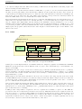
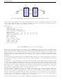
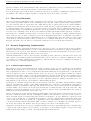
2.4.1
CUDA
Multiprocessor n
...
Multiprocessor 2
Multiprocessor 1
Shared Memory
Instruction
Unit
Registers
Registers
Processor 1
Processor 2
Registers
...
Processor n
Constant and Texture Caches
Device Memory
Fig. 2: The architecture of a typical CUDA GPU.
CUDA [9] is one such implementation of a GPGPU framework, designed by graphics card manufacturer NVIDIA.
Whilst the specifications vary between different cards, a top-spec device will include up to 512 individual cores,
spread over 16 SMPs.
NVIDIA introduce the concept of a block as a collective group of threads. Such threads may work co-operatively,
and are scheduled to the GPU in smaller groups known as warps. Whilst warps may be consider to be a constant
factor from the true execution width of the device, the block may be considered as the grouping of threads that
may semantically co-operate.
Whilst warps are how threads are scheduled to the device, the execution of the warp depends on the device itself.
A CUDA SMP has between 8 and 32 cores, whereas a warp is 32 threads. When a warp is executed, we divide the
32 thread into half or quarter warps. Each smaller group is then executed in parallel on the device - one thread
per core - until the whole warp has been processed.
Such a system ensures that all threads within a warp remain in step. However, since each warp may execute at
its own pace (or that of the scheduler), threads within the same block, but in different warps, may be executing
different pieces of code altogether. NVIDIA provide a __syncthreads() function to ensure all warps reach a given
place in the kernel before continuing.
A SMP provides a large number of registers to all cores - registers are not linked to a given core. The SMP also
provides an on-die area of fast memory, known as shared memory. This shared memory is accessible from all cores
and can be used for co-operative working within a block. Each block may allocate an area of shared memory, and
both read and write to all locations within that area of memory. The memory itself is similar to a L1 cache on a
typical CPU, in that it is close to the processor. In fact, on later devices (those of compute capability 2.0 or above)
a section may be used as a cache from the main memory of the device.
3 Language Design
7
Global Memory is the global-in-scope memory location to which both the host and device can read and write.
It consists of the large part of the device memory advertised for the device - typically in the range of 128Mb or
256Mb for low-end cards, up to 4Gb for specialist workstation cards. Only the host may allocate global memory no dynamic memory allocation is allowed on the device itself. Data may be copied from host-to-device or device-tohost by the host only. However, the device may access the data using a pointer passed as a parameter to the kernel
function. Read/write speeds are in the range of 100GB/s, however they also come at the cost of a high latency
- anywhere between 400 and 800 clock cycles. This memory latency is a conscious design decision - a trade-off
that is often mitigated by providing enough work per SMP so that the scheduler may still make full use of SMP
whilst the memory fetch is occurring. Appropriate algorithms for this type of parallelisation exhibit a high ratio
of arithmetic operations to memory fetch operations.
Since the origins of the multiprocessor in the GPU are in implementing fast hardware pixel shaders, the SMP does
not contain a call stack. We must therefore do away with many of the comforts of programming on a standard
architecture - in particular, all functions are implemented by inlining the definitions in the appropriate places. A
corollary of this approach is that recursive functions cannot be defined directly within CUDA. This condition is
not as onerous as it first appears - in practice, many recursive algorithms will achieve higher performance when
re-written to take advantage of the massive parallelism.
2.5
Prior Work
As a basis for the system, we use the code produced by HMMoC [8], a tool for generating optimised C++ code
for evaluating HMM algorithms, written by Gerton Lunter. This report is considered as the first step to rewriting
HMMoC to utilise the power of desktop GPGPU’s. HMMoC is based upon a HMM file exchange format that uses
XML; the format allows a description of a HMM, and describes which algorithms to generate. It features a generic
macro system and the ability to include arbitrary C. It generates an optimised set of C classes that can be included
by the user in there own projects, providing an efficient HMM implementation.
Other prior work in the area includes BioJava [5], a Java library for Bioinformatics that includes facilities for creating
and executing Hidden Markov Models. Tools for specific HMM problem domains have also been developed. So
called profile HMM’s are one of the main uses within bioinformatics. One of the most popular tools in this area is
HMMER [3].
There are a number of notable elements of prior work to port such HMM applications to GPU architectures.
ClawHMMER [6] was an early attempt to port HMMER to streaming architectures uses the now defunct BrookGPU
[1] programming language. More recent attempts have include GPU-HMMER [11], which instead uses the more
modern NVIDIA CUDA Framework. CuHMM [7] is an implementation of the three HMM algorithms for GPUs,
again using CUDA. It uses a very simple file interchange format, and does not provide native support for HMM’s
with silent states - although the latter restriction can be mitigated through silent state elimination.
3
Language Design
A primary aim of the software tool is to provide the benefits of GPGPU’s to a wider audience. As a result, the
design of the language is vital part of the problem: it must be concise, simple and easy to understand, and prove
itself to be flexible enough to support new formulations as and when they appear. No such general language has
been attempted before, to the best knowledge of the author.
A primary design decision was to assume that the user will not, in any reasonable course of action, be required to
modify the generated code, as in HMMoC. Taking such an approach when faced with generating code for a GPGPU
would reduce the potential audience to such a small group. Instead we take the view that a high-level specification
language is the tool of choice, allowing a wide-variety of users, with a wide-variety of technical expertise, to access
the full power of the GPGPU.
In the following sections we will describe the language through a series of examples, gradually exploring different
areas of the domain.
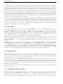
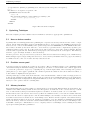
3.1
Occasionally Dishonest Casino
We will first examine a commonly used example - that of the Occasionally Dishonest Casino. The idea here is that
we have a casino that will usually use a regular die, but occasionally they may switch to using a loaded die for a
few turns in order to gain an advantage. A loaded die is one that has been fixed to land on one more faces with a
higher probability than normal. A HMM is an ideal model for this sort of system - we have an output sequence
3 Language Design
8
0.95
1
Start
1:
2:
3:
4:
5:
6:
1/6
1/6
1/6
1/6
1/6
1/6
Fair
0.9
0.05
0.1
1:
2:
3:
4:
5:
6:
1/10
1/10
1/10
1/10
1/10
1/2
End
Loaded
Fig. 3: The Hidden Markov Model representing the Occasionally Dishonest Casino
that is generated by a hidden state - in this case, which die has been chosen. We thus provide two states, one fair
and one loaded. Each state has a set of emission probabilities - the fair is even and the loaded die shows a skew to
certain output characters. Figure 3 is the diagram of the model.
hmm casino {
alphabet [1, 2, 3, 4, 5, 6];
startstate start;
state fair emits fairemission;
state loaded emits loadedemission;
endstate end;
emission fairemission =
[1/6, 1/6, 1/6, 1/6, 1/6, 1/6];
emission loadedemission = [0.1, 0.1, 0.1, 0.1, 0.1, 0.5];
start -> fair 1;
fair -> fair 0.95;
fair -> loaded 0.05;
loaded -> loaded 0.97999;
loaded -> fair 0.02;
loaded -> end 0.00001;
fair -> end 0.00001;
}
Fig. 4: The HMMingbird code for the casino example.
Figure 4 provides a code example for the definition of a casino HMM. We begin with a definition of the hmm element.
We can name our HMM, both as an aid to documentation and for identification purposes. In this case, we have
given it the name casino. Legitimate names may only start with letters, and contain letters or numbers. Any
further description of this model takes place in the form of a series of declarations within the curly brackets {} of
the hmm element. The declarations take place in no particular order. A single program may contain many such hmm
definitions.
The first important declaration is that of the alphabet. This defines the set of valid output characters, separated
by commas, and delimited by squares brackets []. Each element is limited to a single ASCII character in the
current version.
We define the set of states using the state element. We can, and must, specify a single start and end state, using
the appropriate startstate and endstate keywords. We provide every state with a unique name, that can then
be used to define transitions between states. Each state element may define an emisson value using the emits
keyword, that refers to a separate declaration describing the probability distribution over the alphabet. States may
also remain silent by omitting the emits keyword. In this case, we define two regular states - fair and loaded with appropriate emission values - fairemission and loadedemission.
The emission values are simply defined by a list of values corresponding to the order of the alphabet. Each value
is the probability of emission of the character at that position in the alphabet definition. In the fairemission
declaration, all outputs are equally likely, and so are set at 1/6. In the loadedemission declaration, the 6 has a
higher probability, and so the 6th element is set higher. It is desirable for a set of emissions to create a distribution
- in other words, they should sum to 1, as they do for both these cases. However, we do not enforce this restriction
for there may be some cases where a distribution may not be desirable.
Next we describe the structure of the graph by defining the transitions from state to state, with each including an
3 Language Design
9
associated probability that determines how likely the transition is. Just like the emission declaration, it is usually
the case that we want to define a distribution over the transitions from a particular state. If all nodes provide a
distribution over both the emissions and outward transitions, then we have a distribution over the model. This
allows fair comparison between probabilities determined for different sequences. However, as with the emissions,
we do not enforce this rule, allowing a wide range of models to make practical use of the GPGPU.
To produce a completed program we still need to provide a main definition that describes which algorithms should
be run, and on which HMM definitions. We do this with the main keyword. Like the hmm keyword, further
declarations appear within the curly brackets.
main() {
cas = new casino()
dptable = forward(cas);
print dptable.score;
}
The basic declaration here is an assignment; the right hand part must be an expression, the left a new identifier.
The first statement defines an instance of the casino hmm we described above. This syntax will, in future, be
extended to allow parameterisation of the model.
The next step is to perform the algorithm itself. This takes place as a call expression, which uses the name of the
algorithm to run, and passes the HMM as a parameter. In this case, we run the viterbi algorithm with the HMM
cas. We currently support the viterbi, forward and backward algorithms. The parameter to the call is simply
an expression, so we may declare the casino inline like so:
viterbi(new casino());
The result of such a call is returned as the value of that expression. In this case, we have used the variable dptable.
This allows access to the entirety of the dynamic programming table.
Once we have run the algorithm, we need some way to return the results to the user. The print statement acts
as this mechanism, providing a limited system for returning the values in the dynamic programming table. Each
algorithm returns a dynamic programming table with appropriate attributes that we may access. In this case,
the only attribute of the forward algorithm is the score. We can refer to the attribute using a dot notation, as in
dptable.score.
3.2
Profile Hidden Markov Model
A profile hidden markov model is a type of HMM that describes a a family of DNA or protein sequences otherwise
known as a profile [2]. It models the likelihood of a given sequence corresponding to the family described by the
profile, by performing an alignment. An alignment describes the modifications required to change one sequence to
another, which may include inserting characters, deleting characters or matching characters.
This system can be described by a HMM of a certain form. We provide a set of states that represent a single
position in the model, and we can repeat these states any number of times to represent the likelihood of certain
symbols appearing at that position in the sequence. For each position in the model, we may match or delete
that position. Before and after each position, we may introduce characters using the insertion state. Typically,
the model is “trained” using a parameter estimation technique such a Baum-Welch, setting each transition and
emission parameter as appropriate.
HMMER is a popular tool for creating and using profile HMM’s. It uses a custom file format to describe a
parameterised model. We have created a small script that converts the file format to our domain specific language.
We will examine some excerpts here.
As before we declare our model with an appropriate name - we simply use profile here.
hmm profile {
Since we are using protein sequences, this example has the alphabet set to the sequence of valid protein characters.
alphabet [A,C,D,E,F,G,H,I,K,L,M,N,P,Q,R,S,T,V,W,Y];
3 Language Design
10
As in the casino example, we declare a start and end state. We can also see declarations for each position - with
each position containing a insert, delete and match state. Note that the deletion state does not declare the emits
keyword, indicating it is a silent state. It effectively allows the matching process to skip a position.
state D001;
state I001 emits emit_I001;
state M001 emits emit_M001;
We follow that up with the declaration of the emission values for each insert and match state. Although in this
case each state has an individual emission value, in other cases we may share emission values between states.
emission emit_I001 = [0.0681164870327,0.0120080678422,..values ommitted..,0.0269260766547];
emission emit_M001 = [0.0632421444966,0.00530669776362,..values omitted..,0139270170603];
We then describe the set of transitions. We show the transitions for the position 1, but each subsequent position
has a similar set of transitions.
M001
M001
I001
I001
D001
M001
D001
beginprofile
beginprofile
->
->
->
->
->
->
->
->
->
M002
I001
M002
I001
M002
D002
D002
M001
D001
0.985432203952;
0.00980564688777;
0.538221669086;
0.461778330914;
0.615208745166;
0.00476214916036;
0.384791254834;
0.750019494643;
0.249995126434;
One feature used by the profile HMM that has not been previously mentioned is the ability for transitions to include
emission values (Section 2.3.2). We allow this in addition to emissions on states, as there are cases where the most
compact representation will be one notation or the other. They are computationally identical; simply a notational
device. In this case, we emit a character as we transition, and not when arriving at the destination state. We do
not allow both a transition and the destination to emit a character - only one or the other or neither may emit, as
enforced by the compiler. We can then ensure that only a single symbol is emitted at each step through the model.
nterminal
-> nterminalemitter 0.997150581409 emits emit_nterminal_to_nterminalemitter;
In the main definition, we perform the Viterbi algorithm to produce the score of the most likely path, and print
that score using the dot notation as above. However, unlike the casino example, by using the Viterbi algorithm,
we have access to another attribute: traceback. This returns the list of states visited on the most likely hidden
state path. By omitting to access this attribute we cause it not to be evaluated as part of the Viterbi algorithm,
thus increasing efficiency and reducing memory usage.
main() {
dptable = viterbi(new profile());
print dptable.score;
}
By using the simple dot notation we produce just the result - either the final score or the traceback of the optimum
path. But what if we wish to investigate intermediate entries or observe sub-optimal paths? In these cases
we can print the entire dynamic programming table by placing an & at the end of the attribute name like so
dptable.score&. This prints all intermediate results as well as the final score. Note that due to optimisations
within the GPU code, we do not normally store the entirety of the table. Doing so will reduce the number of
sequences that can be processed at any one time, due to the increase in memory requirements.
3.3
Limitations
The definition language described here is somewhat immature at present. We make the following limiting assumptions :
4 Dynamic Programming algorithms for parallel computation
11
• Only a single tape is to be used - multiple tapes are an expected extension. Each tape would contain an
alphabet, and emissions would be linked to particular alphabets;
• Single characters for emission values - in some cases we may require multi-character values;
• Only simple numbers and fractions are allowed in transition and emission probabilities;
4
Dynamic Programming algorithms for parallel computation
The algorithms described in Section 2.2 can all either be implemented with, or make use of, dynamic programming,
a form of optimised computation where we store and reuse intermediate results in order to avoid expensive recomputation. This is possible because the problems exhibit the two key properties required - optimal substructures
and overlapping sub-problems. Computing the probability for a given state relies on computing the value for a set
of previous states with a shortened input - with the result being optimal if all the sub problems are optimal. In
addition, the value for the previous states may be reused for other computations at this position in the input.
There are a number of ways we may implement such a system. One popular method is memoization, where the
result of each function call is stored against the parameters for that call. Further calls with the same parameters
make use of the same result. Whilst this approach can be fruitful within a single thread, it is both difficult
to implement and potentially sub-optimal in a multi-threaded system. In particular, any system that took this
approach would need to ensure that threads had the requisite cross communication and appropriate locking to
ensure duplicate computations of a function call did not take place. This is a particularly difficult task within the
GPU environment, since it neither provides locking facilities nor does it perform optimally when used in this way.
It once again highlights the difference between multi-threading algorithms for CPUs compared to GPUs.
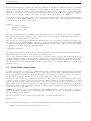
Fortunately, we have another way of implementing a dynamic programming algorithm that is much more suited
to GPUs. A lookup table is a common way of mapping the parameters of a dynamic programming algorithm to
the result of the argument. For most algorithms, the results of all cells in this table will be required at one stage
or another and so we may instead compute the values for this entire table before attempting to compute the final
result, so longs as we ensure any pre-requisites for a given cell are evaluated before the cell itself.
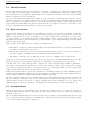
Figure 4 gives a small portion of a dynamic programming table for the casino example described in Section 3.1.
Start
Fair
Loaded
End
Initial
1
0
0
0
’3’
0
1/6
0
0
’1’
0
2.639×10−2
1.389×10−3
0
’6’
0
4.178×10−3
6.805×10−4
0
’6’
0
6.616×10−4
3.334×10−4
0
...
...
...
...
...
Fig. 5: An example of a dynamic programming table for the viterbi trace in the casino example
In a traditional, serial, implementation we would compute each value in this table in turn, ensuring all dependencies
were met before computing a cell. In a parallel implementation, we have a number of options:
Sequence-per-thread We may keep with the same serial algorithm, but compute many such tables at once, relying
on a large input set to keep the device busy. In this case we would allocate a single thread to each sequence.
Sequence-per-block Alternatively, we can use a number of co-operative threads to compute the values in a single
table. Co-operation between threads is required so as to ensure prior dependencies are met before computation
of the current cell can continue.
Sequence-over-MP Finally, we may use a number of co-operative multiprocessors. Such co-operation is currently
difficult to achieve on NVIDIA GPUs. In addition, larger models are required to fully utilise many different
multiprocessors.
Option 1 is suitable for a large number of runs over smaller models. However, if there are a small number of
sequences relative to the number of cores, it is hard to fully utilise the device under this system. In addition, it
cannot necessarily make best use of the caching and localised memory features of the GPU, since each thread is
working independently.
Option 2 is suitable where we can find some way to sensibly divide the work between the different threads on the
GPU. This will rely on a way of identifying dependencies between states to ensure we can parallelise across the
states.
4 Dynamic Programming algorithms for parallel computation
12
Option 3 is trickier on the current hardware. The easiest way to implement cross block communication on current
generation GPUs is to run a separate kernel for each independent set of events.
For our initial approach we will use Option 2, which provides most opportunity for utilising the caching aspects of
the multiprocessor without requiring expensive to-ing and fro-ing from the CPU to the GPU.
4.1
Silent State Elimination
One key problem for parallelisation is the dependencies between states. If we imagine the dynamic programming
table for these algorithms, with the each row marking a state, and each column a position in the output sequence,
we can see that the value at a given state and column may depend on values in the previous column; marking a
transition to the current state from the state in the prior column. We also note that any silent states - those that do
not emit any values - may be referred to by other states in the same column, since no emission has taken place. In
the standard dynamic programming implementation of these algorithms, we would simply ensure all dependencies
were met before evaluating a state. However, in a massively parallel system this is neither practical or desirable.
The solution is to eliminate the silent states, as described in 2.3.3. As it stands, we simply eliminate all silent
states. However, the cost may be mitigated by selectively eliminating silent states. In particular, long paths of
silent states are inefficient in terms of distributing work on a parallel machine, since the length is a lower bound
on the number of iterations required, and so we may choose to eliminate silent states so as to reduce such paths.
The same algorithm can be modified to perform such a task, since we remove silent states iteratively.
4.2
Dynamic Programming: Implementation
It is relatively simple to implement the first approach - thread-per-sequence - as described in Section 4, by taking a
straight-forward serial implementation to run on each individual thread. Nevertheless, by using the elimination of
silent states we can expose an extra dimension of parallelism along the states that will allow a block-per-sequence
approach, which should facilitate an improved use of the device.
Our first implementation of the block-per-sequence algorithm provides a thread for each state in the model. We
thus compute each column in parallel, synchronising after each one. Far more complicated distributions of work
are possible - for example, distributions by transition to different threads - however, for simplicity we will ignore
these extensions for our initial implementation.
4.2.1
A Shared Template Approach
The primary focus for our investigations is the ability of graphics cards to provide a useful speed up for Hidden
Markov Model applications. For the majority of applications the fundamental role which requires acceleration is
that of applying the models to a set of given inputs, rather than training the model parameters to begin with. The
reasons for this are twofold - we usually train the model once and once only, and against a smaller set of inputs
than those that we wish to run it over for the actual application. As such, we will focus for the remaining section
of the paper on the three estimation algorithms: forward, backward and viterbi. We also note that the forward
and backward algorithms play an important role in the baum-welch parameter estimation algorithm, and so the
implementation of the former is a pre-requisite for implementing the latter.
At this stage we can make a useful observation about the nature of the three algorithms - that they all have a similar
structure, and differ only on minor points. This is unsurprising, since each can be, and usually are, implemented
using the dynamic programming lookup approach described in Section 4. The forward and viterbi algorithms are
evidently similar - they traverse the model in an identical way, accessing the same cells at the same time. The
differences lie in how the results from prior cells are combined - with the viterbi algorithm using a max operation,
whilst the forward algorithm sums over the prior cells.
On the other hand, the forward and backward algorithms differ only in the way they traverse the model, not the
way they combine the results. One way of handling the differences in traversal is to provide a modified version of
the model which describes a backward traversal. Such a model is simple to produce within the compiler as a form
of pre-processor. In this case, we can simply use an identical code base to implement the backward algorithm. One
caveat to this approach is the potential cost of duplicating of state and transition data on the device if we require
both the forward and backward algorithms. This cost may be mitigated by combining some invariant aspects of
the model, such as state and emission data, and providing a new version of the transition data.
Using these observations, we can develop a template structure for the three algorithms, that may be parameterised
to support any of them. Figure 6 gives a pseudocode description of the standard template. A by product of this
design decision is the ability to generate other algorithms with a similar pattern.
5 Optimising Techniques
13
{s represents the dynamic programming table, indexed by state and position in sequence}
s = []
for character c in sequence at position i do
parallel for state in states do
sstate,i = 0
for each input transition tj with emission probability ej do
sstate,i = sstate,i op tj ej,c sstartstatetj ,i−1
end for
end for
end for
Fig. 6: The basic shared template
5
Optimising Techniques
The basic template provides a suitable base from which we can start to apply specific optimisations.
5.1
Host to device transfers
A primary issue for CUDA applications is optimising the computational intensity; that is, the ratio of IO to computations. On the authors hardware, memory bandwidth from host to device is pegged at 1600MB/s, whereas device
memory access occur at around 100GB/s, and operational speeds reach 900GFLOP/s for the GT200 architecture.
As a result, both memory allocation and host to device memory copy functions are comparatively expensive, particularly in terms of setup costs. To reduce such costs we take a brute force approach to memory transfer. We first
load the entire sequence file into main memory, then prepare some meta-data about each sequence. The final step
is then to copy both arrays en-masse to the host memory.
Another option is to use page-locked memory allocation, where the host data is never swapped out of main memory.
This technique is quoted as providing twice the host to device memory bandwidth. However, page-locked memory
is a limited resource, and over excessive use may cause slow-down.
5.2
Precision versus speed
A typical problem for applications of this sort is accuracy. The probabilities rapidly become vanishingly small,
often under-flowing the standard floating point data-types, even those of double width. One common approach is
to convert all operations to logspace by computing the log of all the input values, and converting each operation
(max, plus etc.) to the logspace equivalent. We can then represent the values in each cell as either float values, or
double values for slightly increased precision.
One important aspect of this debate is the structure of the current hardware - with a 8:1 ratio for single precision to
double precision instruction throughput, single precision operations can be significantly faster for some applications.
Practical implementations displayed inconsequential differences, in the order of 10%-30%, suggesting that memory
latency for each operation was an overriding issue.
5.3
Memory locations
The CUDA architecture provides a number of disjoint memory locations with different functions and features. For
transition and emission values, which are fixed for all sequences, we make use of the constant memory - a small
area of cached memory that provides fast-as-register access with a one memory fetch cost on a cache miss.
Another fast access location is the shared memory. These are similar in form to a L1 cache in a traditional CPU,
however the allocation is completely user controlled. Each multiprocessor includes one such location, and as such,
it is shared between the blocks allocated to that multiprocessor. Each block has a segment of the shared memory,
which each thread in that block can access. Ideally, we would like to store the dynamic programming tables in this
fast-access memory. However, under the current CUDA architecture the space allocated for each multiprocessor
is 16384Kb. Such space confinements force a low occupancy value for each multiprocessor, resulting in very little
speed up from this particular optimisation.
5 Optimising Techniques
5.4
14
Phased Evaluation
By providing a thread-per-state, we are beholden to the model to determine our block size, since all states share
a block. Since the block-size partly determines the occupancy of a SMP (number of threads per SMP), we may
have an unbalanced set of parameters. Additionally, we are constrained in the size of our models by the maximum
number of threads per block - typically 512.
To remove these unnecessary limitations, we must de-couple the number of threads from the number of states.
The most obvious way to do this is to share a single thread between multiple states, running through the states in
phases. In addition to allowing the block size to become independent of the number of states, this approach has
other benefits. By synchronising the phases across the threads, we can support some form of dependency on the
device - by ensuring that any dependents of a cell are in a prior phase.
5.5
Block size heuristics
One important measure of the effective use of a multiprocessor is the occupancy value - the number of warps per
multiprocessor. Recall that threads are scheduled in warps, 32 threads per warp, so this effectively describes the
number of threads that are active on an SMP at once. Active, in this case, is a statement of resource usage
e.g registers and is does not imply the thread is actually running. A high occupancy plays an important role in
supporting the scheduler to hide the high latency of global memory, by providing many warps to schedule whilst
memory access is in progress.
There are three factors which limit the occupancy of a multiprocessor:
• The number of registers per thread. Each multiprocessor has a limited number of registers, and thus limits
the number of threads that can be placed.
• The amount of shared memory per block. Recall that shared memory is allocated on a per block basis, not
per thread. Again, each multiprocessor has a limited amount of shared memory.
• The number of threads per block. Threads can only be placed on a multiprocessor in entire blocks.
Registers per thread and shared memory per block are both dependent on the kernel implementation alone. The
threads per block is set by a parameter, and is therefore customisable dependent upon the other factors.
It is important to note that achieving a high occupancy is not the be-all-and-end-all of GPGPU optimisation there may be trade-offs when modifying the above factors. For example, we may be able to increase the occupancy
by moving some values from registers to local memory, at the cost of increasing the number of device memory calls
required, which may in fact increase the time taken for the kernel.
Bearing these facts in mind, we can provide a heuristic for determining a suitable block size. NVIDIA provide a
CUDA Occupancy Calculator, which we can use as the basis for computing the values. The calculations used are
described in the CUDA Programming Guide, Chap4: Hardware Impl, pg79.
We take a straight forward approach to implementing the block size heuristics. We try a sequence of likely block
sizes, recording the occupancy for each one. For our candidate block sizes we take multiples of 16 from 16 to 512
plus the number of states. For devices of compute capability 2.0 we check in multiples of 32 - for devices lower
than that warps are executed in half-warps of 16 threads at a time, later devices execute a fall warp at once.
5.6
Unused Attributes
Unused attributes may be both wasteful of space and time. For example, if we do not require the traceback of
the result of the viterbi algorithm, we should not allocate an array in memory for it, nor should we evaluate the
attribute on the device.
We can determine which attributes are used for a given call by providing a program analysis that associates each
use of an attribute with the dynamic programming table. We use that information when generating the CUDA
code to remove unused attributes at compile time.
6 Comparisons
5.7
15
Sliding Window Dynamic Programming Tables
As described in Section 4, we implement the dynamic programming algorithms as a series of lookup tables - with
the states on one axis and the position in the sequence along the top axis. A cell in this table represents the
probability at a given state and position in the table. However, we may not always require these intermediate
results beyond their use for computing other values in the table. This is the case when we have identified partially
used attributes - those where we only require the final value.
In these cases we can economise the table by noting that each of the given algorithms computes the value of a
given cell with reference only to cells in the previous or current columns - since we can have emitted at most one
character at this state. As such, if we do not require the intermediate results, we can implement a sliding window
across the table, storing only the current column and the previous column. At the end of each step we re-designate
the current column as the previous column, and use the previous column as the new current column, overwriting
any previously stored values as we go - cheaply performed using simple pointer manipulation. This mechanism
ensures we store only those values strictly required by the algorithm, thus avoiding excessive memory wastage.
If we consider that each sequence to be evaluated normally requires a O(mn) size table, where m is the number of
states and n the length of the sequence, and a sliding window scheme reduces that to an O(m) we can immediately
see the benefits. Allocating the entire dynamic programming table was therefore a significant area of memory
inefficiency, and resulted in an arbitrary limitation on the number of sequences that could be processed in one run
on the device.
This approach not only has memory allocation benefits, but can also provide improved memory performance by use
of fast-access shared memory. Under the current CUDA architecture the space allocated for each multiprocessor
is just 16384Kb. Such space confinements would allow very few blocks to share a single device, creating a low
occupancy value for each multiprocessor when attempting to store the entire table, reducing the effectiveness
under the normal table allocation scheme. However, under a sliding window, with the significantly reduced memory
requirements, occupancy is not impacted by placing the window in shared memory. The system as implemented
allows models with up to 512 states before the occupancy may be reduced, and even up to 768 may be safely
accommodated before occupancy is reduced below the 25% level recommended by NVIDIA.
Whilst this is successful in reducing the memory usage, it does mean that we are unable to recreate the backtracking
trace through the table. This can be rectified by allocating a separate table to store the backtracking data for
each cell - a table that is of a smaller size than the full table since each cell only needs to store the position of
the previous cell, and not a complete floating point number. In most cases, the number of states - the number of
possible prior positions - requires fewer bits than a full 32 bit float. For the forward and backward algorithms no
backtracking is required, and so there is no need for this extra storage.
5.8
Custom kernels for each program call
For each algorithm call in the program, we generate a different kernel call using customised kernel code. Doing so
allows allows the removal of a number of unnecessary runtime checks.
• We generate different code depending on the specified block size. If the block size that has been determined
(see Section 5.5) is smaller than the number of states, each thread needs to iterate over the assigned states.
This code is only generated in that case.
• For each call we determine which attributes are required - and in what form - and only generate the code to
store the attributes accessed (see Section 5.6). Since we determine whether we require simply the end result
or the entirety of the table, we can generate code that stores the intermediate results or accumulates the
attribute without storing it (see Section 5.7).
5.9
Sorting Input
One observation we make is that a pre-sorted input sequence will have a more optimal execution pattern. This is
an optimisation that was also noted in GPU-HMMER [11].
6
6.1
Comparisons
The Occasionally Dishonest Casino
We describe the casino model in Section 3.1. It has been chosen as a simple example of a Hidden Markov Model.
6 Comparisons
16
No. of Seq.
2500
5000
7500
10000
HMMingbird
0.126
0.149
0.206
0.222
HMMoC1.3
2.611
5.526
8.406
11.028
Speed Up
20.72
37.09
40.81
49.68
Fig. 7: HMMingbird versus HMMoC1.3 on the Occasionally Dishonest Casino
As a simple test for speed versus HMMoC we use a set of pre-generated sequences of various lengths.
6.2
Profile Hidden Markov Model
The structure of a profile hidden markov model is described in Section 3.2.
A profile HMM is one of the most widely used applications for HMM within bioinformatics. HMMER is a tool
that can create profile HMM’s and use them to search vast databases of sequences. It has been in development
for over fifteen years, and is highly optimised. In particular, it uses forms of corner cutting to remove swathes of
computations. Various attempts have been made to port HMMER to use GPU’s. The most widely known example
is GPU-HMMER [11], which provides a CUDA based mechanism for searching databases.
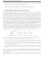
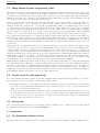
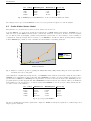
7
Time in Seconds
6
5
4
HMMingbird
HMMer2
GPU-HMMeR
3
2
1
0
5000
13355
25000
50000
75000
Number of Sequences
Fig. 8: Chart for a 10 state profile recognising the Thymidine kinase (TK) family, using the viterbi algorithm to
determine the best scoring path.
Our results show a significant (x2-x4) increase over HMMER, in line with the performance gains shown by GPUHMMER. It is particularly worth noting that GPU-HMMER is a hand-coded and optimised application for a
specific subset of HMM’s, yet HMMingbird outperforms it by between 15%-45% in these tests. Examining the two
programs under a profiler suggests that GPU-HMMER has a faster kernel, however this is offset by an inefficient
data transfer process. Another note of caution is that GPU-HMMER does some post-processing, which may also
account for some of the difference.
No. of Seq.
5000
13355
25000
50000
75000
HMMoC1.3
4.809s
25.68s
49.548s
90.8s
168.376s
HMMingbird
0.161s
0.449s
0.65s
1.111s
1.638s
Speed Up
x29.87
x57.19
x76.23
x81.73
x102.79
Fig. 9: Speed up versus HMMoC
We also see significant performance gains when compared to HMMoC, with greater gains as we evaluate larger and
larger sequence databases.
7 Conclusions
7
17
Conclusions
Our tool significantly improves on prior work in two important areas:
• By providing a concise language for describing Hidden Markov Models. It is significantly shorter and clearer
than the equivalent descriptions for general purpose tools such as HMMoC.
• Demonstrates clear increases over CPU only methods on computation, and performance on-par with other
GPU tools, with a wider range of input models.
Previous attempts to describe Hidden Markov Models have been focused on producing a file interchange format
for models, and as such they have been focused on formats that have readily available means for parsing, such as
XML or S-Expressions. Whilst these techniques reduce the difficulty of building the tool, they do not make it easy
for the user, nor do they provide an elegant way of specifying the models.
By taking a different approach that focuses on the Hidden Markov Models as programs not data, we can bring to
bear a whole range of tools and techniques to aid in both the implementation and the design of a domain specific
language. Doing so changes the expectations we have for the language - the tool is no longer a code generator but
a fully-fledged compiler. We can approach the problem with a clean and clear syntax - removing any loopholes
such as the inclusion of arbitrary C code. This allows us to focus on generating the best possible GPU code,
without worrying about user changes - sacrificing some flexibility for usability. This is a particularly important
consideration when trying to tempt a broad spectrum of users to the tool.
Our performance results prove the effectiveness of dynamic programming algorithms of this ilk on massively parallel
architectures. Despite the intrinsic dependencies within the algorithm - it is not trivial to parallelise - we can
produce fast code, with plenty of scope for improvement.
8
Further Work
Whilst we believe we have excellent performance using the current system for large number of sequences on small
to medium size model, we wish to improve our performance on both larger and smaller models. In particular,
we would like to implement different models of division of labour for models with sizes at either extremity. For
small models, a sequence-per-thread distribution should increase performance by reducing the co-operation required
between threads, at the cost of increasing register usage per kernel. For larger models - say tens of thousands of
states - we might wish to implement a cross-block system, where each kernel call computes one column in the table
using multiple blocks.
A further modification to support large models with a linear structure is to allow some silent states within the
model. The current mechanism removes all silent states during compilation. In linear structures this may cause an
exponential growth in the number of transitions. By allowing some silent states, we can reduce this growth. The
caveat is that we must ensure the kernel computes all silent states before emitting states. This can be fixed by
ensuring that the silent states are at the start of the state array, and that their dependents are at the end of the
state array. We can then set block size appropriately, so that the blocks with silent states are computed prior to
the blocks with dependent states.
Under the block-per-sequence model, we often find divergence due to the varying number of transitions per state.
We also find memory bank conflicts and constant cache conflicts when more than one thread a) accesses the same
location in shared memory; or b) accesses different locations in the constant cache. Reduction of conflicts can come
from ordering the transitions appropriately to reduce such issues. In addition, we can modify our algorithm to
separate states from threads, so each thread can support multiple states. This allows a grouping of states in a
single thread to smooth out differences in the number of transitions between threads.
Generalising the work described in Section 4, we hope to develop a small functional language that will allow the
differences between the three algorithms to be described in terms of the recursions they implement. Furthermore,
we hope to widen the scope of such a language to encompass other such dynamic programming algorithms with
similar characteristics.
References
[1] I. Buck, T. Foley, D. Horn, J. Sugerman, K. Fatahalian, M. Houston, and P. Hanrahan. Brook for gpus:
stream computing on graphics hardware. ACM Trans. Graph., 23(3):777–786, August 2004.
8 Further Work
18
[2] R. Durbin, S. R. Eddy, A. Krogh, and G. Mitchison. Biological Sequence Analysis: Probabilistic Models of
Proteins and Nucleic Acids. Cambridge University Press, July 1999.
[3] S. Eddy. HMMer Website, including User Manual. http://hmmer.wustl.edu.
[4] H. Ito, S. Amari, K. Kobayashi. Identifiability of hidden Markov information sources and their minimum
degrees of freedom. IEEE Transactions on Information Theory, 38(2):324–333, March 1992.
[5] R. C. G. Holland, T. Down, M. Pocock, A. Prlic, D. Huen, K. James, S. Foisy, A. Drager, A. Yates, M. Heuer,
and M. J. Schreiber. Biojava: an open-source framework for bioinformatics. Bioinformatics, 24(18):btn397–
2097, August 2008.
[6] D. R. Horn, M. Houston, and P. Hanrahan. Clawhmmer: A streaming hmmer-search implementatio. In
Proceedings of the 2005 ACM/IEEE conference on Supercomputing, SC ’05, pages 11–, Washington, DC,
USA, 2005. IEEE Computer Society.
[7] C. Liu.
cuHMM: a CUDA Implementation of Hidden Markov Model Training and Classification.
http://liuchuan.org/pub/cuHMM.pdf, 2009.
[8] G. Lunter. HMMoC a compiler for hidden Markov models. Bioinformatics, 23(18):2485–2487, September
2007.
[9] NVIDIA. NVIDIA CUDA Programming Guide, Version 3.0. February 2010.
[10] Ulrich Faigle and Alexander Schoenhuth. A simple and efficient solution of the identifiability problem for
hidden Markov processes and quantum random walks. 2008.
[11] J. P. Walters, V. Balu, S. Kompalli, and V. Chaudhary. Evaluating the use of gpus in liver image segmentation
and hmmer database searches. In IPDPS ’09: Proceedings of the 2009 IEEE International Symposium on
Parallel&Distributed Processing, pages 1–12, Washington, DC, USA, 2009. IEEE Computer Society.