No category

Download GPU computations in heterogeneous grid

Transcript

GPU COMPUTATIONS IN
HETEROGENEOUS GRID
ENVIRONMENTS
Marcus Hinders
Master of Science Thesis
Supervisor: Jan Westerholm
Department of Information Technologies
Åbo Akademi University
December 2010
A BSTRACT
This thesis describes how the performance of job management systems on heterogeneous computing grids can be increased with Graphics Processing Units (GPU). The
focus lies on describing what is required to extend the grid to support the Open Computing Language (OpenCL) and how an OpenCL application can be implemented for
the heterogeneous grid. Additionally, already existing applications and libraries utilizing GPU computation are discussed.
The thesis begins by presenting the key differences between regular CPU computation and GPU computation from which it progresses to the OpenCL architecture.
After presenting the underlying theory of GPU computation, the hardware and software requirements of OpenCL are discussed and how these can be met by the grid
environment. Additionally a few recommendations are made how the grid can be configured for OpenCL. The thesis will then discuss at length how an OpenCL application
is implemented and how it is run on a specific grid environment. Attention is paid to
details that are impacted by the heterogeneous hardware in the grid.
The theory presented by the thesis is put into practice by a case study in computational biology. The case study shows that significant performance improvements are
achieved with OpenCL and dedicated graphics cards.
Keywords: grid job management, OpenCL, CUDA, ATI Stream, parallel programming
i
P REFACE
The research project, of which this thesis is a product, was a collaboration between
Åbo Akademi University and Techila Technologies Ltd. I would like to thank for the
assistance and guidance provided by professor Jan Westerholm and PhD student Ville
Timonen at Åbo Akademi. I would also like to thank CEO Rainer Wehkamp and R&D
Director Teppo Tammisto of Techila Technologies for their support during the research
project.
ii
C ONTENTS
Abstract
i
Preface
ii
Contents
iii
List of Figures
v
List of Tables
vii
List of Algorithms
viii
Glossary
ix
1
Introduction
1
2
GPU computation
2.1 Graphics cards as computational devices
2.2 Frameworks . . . . . . . . . . . . . . .
2.3 Algorithms suitable for the GPU . . . .
2.3.1 Estimating performance gain . .
.
.
.
.
3
4
6
7
8
.
.
.
.
.
.
9
9
11
11
13
14
15
.
.
.
.
16
16
18
20
22
3
4
Grid and OpenCL architecture
3.1 Techila Grid architecture . .
3.2 OpenCL architecture . . . .
3.2.1 Platform model . . .
3.2.2 Execution model . .
3.2.3 Memory model . . .
3.2.4 Programming model
.
.
.
.
.
.
.
.
.
.
.
.
.
.
.
.
.
.
.
.
.
.
.
.
.
.
.
.
.
.
.
.
.
.
.
.
.
.
.
.
.
.
.
.
.
.
.
.
.
.
.
.
.
.
.
.
.
.
.
.
.
.
.
.
.
.
.
.
.
.
.
.
.
.
.
.
Grid client requirements and server configuration
4.1 Hardware requirements . . . . . . . . . . . . .
4.2 Software requirements . . . . . . . . . . . . .
4.2.1 Operating system constraints . . . . . .
4.3 Grid server configuration . . . . . . . . . . . .
iii
.
.
.
.
.
.
.
.
.
.
.
.
.
.
.
.
.
.
.
.
.
.
.
.
.
.
.
.
.
.
.
.
.
.
.
.
.
.
.
.
.
.
.
.
.
.
.
.
.
.
.
.
.
.
.
.
.
.
.
.
.
.
.
.
.
.
.
.
.
.
.
.
.
.
.
.
.
.
.
.
.
.
.
.
.
.
.
.
.
.
.
.
.
.
.
.
.
.
.
.
.
.
.
.
.
.
.
.
.
.
.
.
.
.
.
.
.
.
.
.
.
.
.
.
.
.
.
.
.
.
.
.
.
.
.
.
.
.
.
.
.
.
.
.
.
.
.
.
.
.
.
.
.
.
5
Libraries and applications utilizing GPU computation
5.1 Linear algebra libraries . . . . . . . . . . . . . . . . . . . . . . . . .
5.2 Matlab integration . . . . . . . . . . . . . . . . . . . . . . . . . . . .
24
24
26
6
Implementing a Techila Grid OpenCL application
6.1 Local control code . . . . . . . . . . . . . . .
6.2 OpenCL worker code . . . . . . . . . . . . . .
6.2.1 OpenCL host code . . . . . . . . . . .
6.2.2 OpenCL kernels . . . . . . . . . . . .
6.2.3 Profiling and debugging . . . . . . . .
7
8
.
.
.
.
.
.
.
.
.
.
.
.
.
.
.
.
.
.
.
.
.
.
.
.
.
.
.
.
.
.
.
.
.
.
.
.
.
.
.
.
.
.
.
.
.
.
.
.
.
.
.
.
.
.
.
.
.
.
.
.
28
28
31
31
38
42
Case study
7.1 The Gene Sequence Enrichment Analysis method
7.2 Parallelization with OpenCL . . . . . . . . . . .
7.3 Test environment . . . . . . . . . . . . . . . . .
7.4 Test results . . . . . . . . . . . . . . . . . . . .
7.4.1 Overall comparison of performance . . .
7.4.2 Comparison of OpenCL performance . .
.
.
.
.
.
.
.
.
.
.
.
.
.
.
.
.
.
.
.
.
.
.
.
.
.
.
.
.
.
.
.
.
.
.
.
.
.
.
.
.
.
.
.
.
.
.
.
.
.
.
.
.
.
.
.
.
.
.
.
.
.
.
.
.
.
.
44
44
46
52
53
54
58
Conclusions
62
Bibliography
64
Swedish summary
68
A Appendices
A.1 Case study execution times . . . . . . . . . . . . . . . . . . . . . . .
73
73
iv
L IST OF F IGURES
2.1
2.2
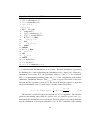
Development of peak performance in GPU:s and CPU:s in terms of
billions of floating point operations per second (GFLOPS) [1]. . . . .
Differences in GPU and CPU design. Green color coding is used for
ALUs, yellow for control logic and orange for cache memory and
DRAM [2]. . . . . . . . . . . . . . . . . . . . . . . . . . . . . . . .
Techila Grid infrastructure [3]. . . . . . . . . .
Techila Grid process flow [4]. . . . . . . . . . .
OpenCL platform model [5]. . . . . . . . . . .
Example of a two dimensional index space [5].
OpenCL memory model [5]. . . . . . . . . . .
.
.
.
.
.
10
10
12
13
15
4.1
The OpenCL runtime layout. . . . . . . . . . . . . . . . . . . . . . .
19
6.1
6.2
Techila grid local control code flow [6]. . . . . . . . . . . . . . . . .
Example of OpenCL host code flow. . . . . . . . . . . . . . . . . . .
29
33
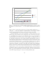
7.1
Execution times of GSEA algorithm implementations on Worker 2
when the length of L is increased and m = 500. The OpenCL implementations utilize the GPU. . . . . . . . . . . . . . . . . . . . . .
Execution times of GSEA algorithm subsections on Worker 2 when the
length of L is increased and m = 500. The OpenCL implementations
utilize the GPU. . . . . . . . . . . . . . . . . . . . . . . . . . . . . .
Execution times of GSEA algorithm implementations on Worker 2
when the size of S is increased and n = 15000. The OpenCL implementations utilize the GPU. . . . . . . . . . . . . . . . . . . . . .
Execution times of GSEA algorithm subsections on Worker 2 when
the size of S is increased and m = 500. The OpenCL implementations
utilize the GPU. . . . . . . . . . . . . . . . . . . . . . . . . . . . . .
Total execution times of the GSEA algorithm OpenCL implementations on different GPUs when the length of L is increased and m = 500.
Subsection execution times of the GSEA algorithm OpenCL implementations on different GPUs when the length of L is increased and
m = 500. . . . . . . . . . . . . . . . . . . . . . . . . . . . . . . . .
7.3
7.4
7.5
7.6
v
.
.
.
.
.
.
.
.
.
.
.
.
.
.
.
.
.
.
.
.
.
.
.
.
.
.
.
.
.
.
.
.
.
.
.
.
.
.
.
.
.
.
.
.
.
.
.
.
.
.
5
3.1
3.2
3.3
3.4
3.5
7.2
.
.
.
.
.
4
55
56
56
57
58
59
7.7
7.8
Total execution times of the GSEA algorithm OpenCL implementations on different GPUs when the size of S is increased and n = 15000. 60
Subsection execution times of GSEA algorithm OpenCL implementations on different GPUs when the size of S is increased and n = 15000. 60
vi
L IST OF TABLES
2.1
Indicative table of favorable and non-favorable algorithm properties. .
7
4.1
Hardware accessible under different operating systems [7, 8]. . . . . .
20
7.1
Test environment grid workers . . . . . . . . . . . . . . . . . . . . .
53
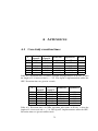
A.1 Execution times of GSEA algorithm implementations on Worker 2
when the length of L is increased and m = 500. The OpenCL implementations utilize the GPU. Execution times are given in seconds. .
A.2 Execution times of GSEA algorithm subsections on Worker 2 when the
length of L is increased and m = 500. The OpenCL implementations
utilize the GPU. Execution times are given in milliseconds. . . . . . .
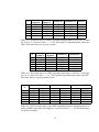
A.3 Execution times of GSEA algorithm implementations on Worker 2
when the size of S is increased and n = 15000. The OpenCL implementations utilize the GPU. Execution times are given in seconds. .
A.4 Execution times of GSEA algorithm subsections on Worker 2 when
the size of S is increased and m = 500. The OpenCL implementations
utilize the GPU. Execution times are given in milliseconds. . . . . . .
A.5 Total execution times of the GSEA algorithm OpenCL implementations on different GPUs when when the length of L is increased and
m = 500. Execution times are given in seconds. . . . . . . . . . . . .
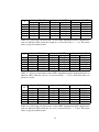
A.6 Subsection execution times of the GSEA algorithm OpenCL implementations on different GPUs when the length of L is increased and
m = 500. Execution times are given in milliseconds. . . . . . . . . .
A.7 Total execution times of the GSEA algorithm OpenCL implementations on different GPUs when the size of S is increased and n = 15000.
Execution times are given in seconds. . . . . . . . . . . . . . . . . .
A.8 Subsection execution times of the GSEA algorithm OpenCL implementations on different GPUs when the size of S is increased and
n = 15000. Execution times are given in milliseconds. . . . . . . . .
vii
73
73
74
74
74
75
75
75
L IST OF A LGORITHMS
1
2
3
4
5
Pseudocode of GSEA . . . . . . . . . . . .
Pseudocode ofcalculateES function . . . .
Pseudocode of the ismember function . . .
Pseudocode of optimized ismember function
Pseudocode of Knuth’s shuffle . . . . . . .
viii
.
.
.
.
.
.
.
.
.
.
.
.
.
.
.
.
.
.
.
.
.
.
.
.
.
.
.
.
.
.
.
.
.
.
.
.
.
.
.
.
.
.
.
.
.
.
.
.
.
.
.
.
.
.
.
.
.
.
.
.
.
.
.
.
.
.
.
.
.
.
45
46
47
48
49
G LOSSARY
CUDA
Compute Unified Device Architecture is a hardware architecture and a software
framework of Nvidia, enabling of GPU computation.
ATI Stream
ATI Stream is AMD’s hardware architecture and OpenCL implementation enabling GPU computation.
OpenCL
Open Computing Language is a non-proprietary royalty free GPU computing
standard.
NDRange, global range
A index space defined for the work to be done. The index space dimensions are
expressed in work-items.
work-group
A group of work-items.
work-item
A light-weight thread executing kernel code.
kernel
A function that is executed by a compute device.
host device
Device that executes the host code that controls the compute devices.
compute device
A device that executes OpenCL kernel code.
ix
compute unit
A hardware unit, consisting of many processing elements, that executes a workgroup.
processing element
A hardware unit that executes a work-item.
grid client, grid worker
A node in a computational grid that performs jobs assigned to it.
grid server
A server that distributes jobs to grid clients and manages them.
grid job
A small portion of an embarassingly parallel problem executed by a worker.
worker code
An application binary that is to be executed on a worker.
local control code
Code that manages the grid computation and is executed locally.
x
1 I NTRODUCTION
In high performance computing there is a constant demand for increased computational processing power as applications grow in complexity. A lot of research is done
in the field of high performance computing and from that research new technologies
such as Graphics Processing Unit (GPU) computing have emerged. GPU computing
is gaining increasing interest due to its great potential. Because GPU computing is a
relatively new technology it is not always clear however when it could be used and
what kind of problems will gain from its usage. This thesis tries to bring light on
this matter. The main obstacle for deploying GPU computation today is the new way
of thinking required by the application developer. Most developers are accustomed
to single threaded applications, but even those who are familiar with parallel programming using the Open Multi-Processing (OpenMP) or Message Passing Interface (MPI)
application programming interfaces (API) will notice significant differences in architecture and way of programming. Due to these differences this thesis will present the
Open Compute Language (OpenCL) and how an OpenCL application is implemented.
This is done as part of a greater endeavor to investigate how a commercially available
grid job management system, the Techila grid, can be extended to support GPU computation. The thesis assumes a grid with heterogeneous GPU hardware, but will not
discuss any modifications of the grid middleware. The hardware and software requirements presented by this thesis and the usefulness of GPU computation in the Techila
grid is assessed in practice through a case study.
Chapter 2 of this thesis gives an overlook of GPU computation. The key differences between CPUs and GPUs are presented as well as different frameworks and
their origin. This chapter provides also a general view on what kind of algorithms are
suited for GPU computation. Chapter 3 presents the architecture of the Techila grid
and OpenCL in order to give a basic understanding of the system structure needed in
chapter 6. OpenCL support is not an integrated part of the Techila grid or the majority
of operating systems. Chapter 4 describes in detail which steps have to be taken in
1
order to extend a grid to support OpenCL. This chapter also presents the constraints
that prevent the use of OpenCL in some cases. Chapter 6 is dedicated to describing
how an OpenCL application that is to be run on the grid should be implemented and
how the OpenCL grid computation can be managed. The performance of an OpenCL
implementation compared to a regular C language implementation and a Matlab implementation is evaluated in chapter 7, where a set of tests are performed as part of a
case study. Chapter 8 will discuss the findings of this thesis.
2
2 GPU COMPUTATION
In the past a common approach to increase the processing power of a Central Processing Unit (CPU) was to increase the clock frequency of the CPU. After some time
the heat dissipation became a limiting factor for this approach and CPU manufacturers
changed their approach to the problem by adding computational cores to their CPUs
instead of increasing the clock frequency. Desktop computers today commonly have
2-6 computational cores in their CPU. The next major step in increasing the computational power will most likely be heterogeneous or hybrid computing. Heterogeneous
computing is a term used for systems utilizing many different kinds of computational
units for computations. These computational units could be CPUs, hardware accelerators or Graphics Processing Units (GPU), to mention a few. When one or more GPUs
and CPUs are used in combination to perform general purpose calculations it is called
GPU computing. In the literature the more established term General Purpose computing on GPUs (GPGPU) is also commonly used as a synonym for GPU computing.
Some sources use GPGPU as the term for general purpose computing mapped against
a graphics application programming interfaces (API) such as DirectX or OpenGL [1].
In this thesis the term GPU computing will be used instead of the slightly indefinite
GPGPU.
The first section of this chapter will present the main differences between a CPU
and a GPU from a hardware point of view. The second section will discuss the evolution of GPU computing software frameworks. The third and final section presents
different aspects of GPU computation that should be considered before parallelizing
code for the GPU. The final section also reminds the reader of the general methods that
can be used to estimate the speedup factor achieved by parallelizing an algorithm.
3
p��7�
In contrast, the many-core trajectory focuses more on the execution
throughput of parallel applications. The many-cores began as a large number of much smaller cores, and, once again, the number of cores doubles
with each generation. A current exemplar is the NVIDIA� GeForce�
GTX 280 graphics processing unit (GPU) with 240 cores, each of which
is a heavily multithreaded, in-order, single-instruction issue processor that
shares its control and instruction cache with seven other cores. Many-core
processors, especially the GPUs, have led the race of floating-point perfor2.1 since
Graphics
cards
as computational
mance
2003. This
phenomenon
is illustrated devices
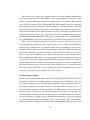
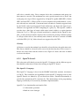
in Figure 1.1. While the
performance improvement of general-purpose microprocessors has slowed
GPU computing has gained momentum during the past years because of the massively
significantly, the GPUs have continued to improve relentlessly. As of
parallel processing power a single GPU contains compared to a CPU. A single high
2009, the ratio between many-core GPUs and multicore CPUs for peak
end graphics card
currently has
roughly tenistimes
floating
floating-point
calculation
throughput
aboutthe10single
to 1.precision
These are
not point
necesprocessing
capability
of
a
high
end
CPU
while
the
price
is
roughly
the
same.
Thethe
sarily achievable application speeds but are merely the raw speed that
processing power
of the can
CPUspotentially
has increasedsupport
according
Moore’s
law [9],
it is
execution
resources
intothese
chips:
1 but
teraflops
outpaced
by the GPUs’
increase
in processing
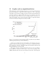
power. Figure 2.1 depicts the tremend(1000
gigaflops)
vs. 100
gigaflops
in 2009.
DO NOT DISTRIBUTE- COPYRIGHTED MA
ous increase in GPU processing power since the year 2002.
1200
1000
AMD (GPU)
NVIDIA (GPU)
Intel (CPU)
Many-core GPU
GFLOPS
800
600
400
200
Multicore CPU
dual-core
0
2001
f��1�
2002
2003
2004
2005
Year
2006
quad-core
2007 2008 2009
Courtesy: John Owens
FIGURE
1.1 Development of peak performance in GPU:s and CPU:s in terms of billions
Figure 2.1:
of floatingperformance
point operations
second (GFLOPS)
Enlarging
gapperbetween
GPUs and[1].
CPUs.
Another aspect working in the favor of the graphics cards is their low energy consumption compared to their processing power. For instance an AMD Phenom II X4
CPU operating at 2.8 GHz has a GFLOPS to Watts ratio of 0.9 while a mid-class ATI
Kirk-Hwu�
Radeon 5670 GPU has a ratio of 9.4
[10]. 978-0-12-381472-2
GPUs deploy a hardware architecture that Nvidia calls Single Instruction Multiple
Thread (SIMT) [2]. Modern x86 CPUs deploy a Single Instruction Multiple Data
(SIMD) architecture that issues the same operation on data vectors. The focal point
Uncorrected proofs - for course adoption rev
4
of the SIMT architecture is the thread that executes operations, while the SIMD architecture is focused around the data vectors and performing operations on them [11].
In the SIMT architecture groups of lightweight threads execute in lock-step a set of
instructions on scalar or vector datatypes. The groups of lightweight threads are called
warps or wavefronts. The term warp is used in reference to CUDA and consists of
32 threads, while a wavefront consist of 64 threads and is used in connection with the
ATI Stream architecture. All threads in the group have a program counter and a set of
private registers that allow them to branch independently. The SIMT architecture also
enables fast thread context switching which is the primary mechanism for hiding GPU
Dynamic Random Access Memory (DRAM) memory latencies. GPUs and CPUs differ
in their design primarily by the different requirements imposed upon them. Graphics
cards are first and foremostly intended for graphics objects and pixel processing that
requires thousands of lightweight hardware threads, high memory bandwidth and little
�
��
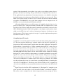
control flow. CPUs on the other hand are mostly designed with sequential general
purpose processing in mind. CPUs have few hardware threads, large cache memories
to� keep the memory latency low and advanced control flow logic. New CPUs sold
on
today’s market have commonly 4-12 MB of cache memory in three levels while the
��
��
best
graphics cards have less than 1 MB of cache in two levels [12]. The cache memory
��
and the advanced control flow logic require a lot of space on a silicon die, which in the
��
GPU
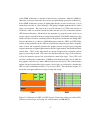
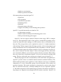
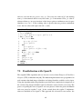
is used for additional arithmetic logical units (ALU). The schematic of figure 2.2
��
shows the conceptual differences in processing unit design.
�
��
��
��
��
��
�
�
�
�
�
�
�
�
��
��
��
��
��
�
Figure
2.2: Differences
in GPU and CPU design. Green color coding is used for ALUs,
��
��
yellow for control logic and orange for cache memory and DRAM [2].
��
�
��
5
��
��
��
��
��
��
2.2
Frameworks
At the end of 1990s graphics cards had fixed vertex shader and pixel shader pipelines
that could not be programmed [1]. This changed however with the release of DirectX 8 and the OpenGL vertex shader extension in 2001. Pixel shader programming
capabilities followed a year later with DirectX 9. Programmers could now write their
own vertex shader, geometry shader and pixel shader programs. The vertex shader
programs mapped vertices, i.e. points, into a two dimensional or three dimensional
space, while geometry shader programs operated on geometric objects defined by several vertices. The pixel shader programs calculate the color or shade of the pixels. At
this time programmers that wanted to utilize the massively parallel processing power
of their graphics cards to express their general purpose computations in terms of textures, vertices and shader programs . This was not particularly easy nor flexible and in
November 2006 both Nvidia and ATI released their proprietary frameworks specifically aimed for GPU computing. Nvidia named its framework Compute Unified Device
Architecture (CUDA) [13]. The CUDA framework is still today under active development and used in the majority of GPU computations. Besides the OpenCL API,
CUDA supports four other APIs: CUDA C, CUDA driver API, DirectCompute and
CUDA Fortran. CUDA C and CUDA driver APIs are based upon the C programming
language. DirectCompute is an extension of graphics API DirectX and CUDA Fortran
is a Fortran based API developed as a joint effort by Nvidia and the Portland Group.
ATI’s framework was called Close-to-the-metal (CTM) which gave low-level access
to the graphics card hardware [14]. The CTM framework later became the Compute
Abstract Layer (CAL). In 2007 ATI introduced a high-level C-based framework called
ATI Brook+ which was based upon the BrookGPU framework developed by Stanford
University. The BrookGPU framework was a layer built on top of graphics APIs such
as OpenGL and DirectX, to provide the programmers high-level access to the graphics hardware and was thus the first none-proprietary GPU computing framework. ATI
Brook+ however used CTM to access the underlying hardware.
In 2008 both Nvidia and AMD joined the Khronos group in order to participate
in the development of an industry standard for hybrid computing. The proposal for
the royalty free Open Computing Language (OpenCL) standard was made by Apple
Inc. and version 1.0 of the OpenCL standard was ratified in December 2008 and is
the only industry standard for hybrid computing to date. OpenCL version 1.1 was
released in August 2010. In this thesis GPU Computing is discussed from the OpenCL
6
perspective because it is better suited for grid environments. The CUDA Driver API
and the OpenCL API are very similar to their structure and many of the concepts
discussed in this thesis apply also to CUDA C and the CUDA driver API.
2.3
Algorithms suitable for the GPU
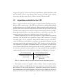
Table 2.1 shows an indicative list of favorable and non-favorable algorithm properties
from the GPU’s point of view. The GPU is well suited for solving embarrassingly
parallel problems due to its SIMT architecture. Embarrassingly parallel problems are
problems that can be divided into independent tasks that do not require interaction with
each other. Data can however be shared to a limited extent between threads on a GPU,
but the threads should have as few data dependencies to each other as possible. The
sharing of data between threads is explained in more detail in section 3.2.3.
The most important aspect in terms of performance is high arithmetic logical unit
utilization. The factor that most significantly impacts GPU utilization is diverging
execution paths, i.e if-else statements. When threads within a warp or wavefront diverge, the different execution paths are serialized. An algorithm with many divergent
execution paths will thus not perform well on a GPU. Another factor that affects the
ALU utilization is the graphics card DRAM memory access patterns. A scattered data
access pattern will start many fetch operations that decrease performance as graphics cards have small or no cache memories. It is also beneficial if the algorithm is
computationally intensive as this will hide the graphics card DRAM access latencies.
Favorable property
Embarrassingly parallel
Computationally intensive
Data locality
Non-favorable property
Many divergent execution paths
Input/Output intensive
High memory usage (> 1GB)
Recursion
Table 2.1: Indicative table of favorable and non-favorable algorithm properties.
The memory resources of graphics cards are limited. When an application has
allocated all graphics card DRAM the data is not swapped to central memory or the
hard disk drive as with regular applications. Furthermore when the data is transferred
from central memory to dedicated graphics cards it has to pass through the Peripheral
Component Interconnect Express (PCIe) bus, that has a theoretical transfer rate of 8
7
GBps [10]. Due to this low bandwidth of the PCIe bus compared to the graphics card
DRAM and central memory it becomes a performance limiting factor and therefore
transfers over the PCIe bus should be kept to a minimum [15]. From this it follows that
input and output intensive algorithms are not suited for GPU computation as they will
cause intensive data transfers on the PCIe bus. Additional non-favorable properties are
file and standard input or output operations that cannot be performed by code running
on the GPU.
2.3.1
Estimating performance gain
Amdahl’s law given by equation 2.1 presents a means to estimate the speed-up S of
a fixed sized problem [11]. T (1) is the execution time of the whole algorithm on one
processor core and T (N ) is the execution time of the parallelized algorithm on N
processor cores. The execution time T (N ) can be expressed as the execution time of
the sequential section Ts and the execution time of the parallel section Tp run on one
processor core divided by the number of cores N . As a GPU utilizes tens of thousands
of lightweight threads for processing the equation can be simplified by having N go to
infinity, which yields equation 2.2.
S=
S = lim
N →∞
Ts + Tp
T (1)
=
T (N )
Ts + TNp
Ts + Tp
Ts +
Tp
N
!
=1+
(2.1)
Tp
Ts
(2.2)
Amdahl’s law assumes that the number of threads N and the execution time of the
parallel section Tp are independent, which is in most cases not true. Gustafson’s law
[16] shows that the execution time is kept constant if the problem size and the number
of threads are increased. This observation is important in GPU computation where
in many cases a larger problem size is more desirable than speeding up a fixed sized
problem.
8
3 G RID AND O PEN CL ARCHITECTURE
This thesis will study the possibilities of utilizing OpenCL in the commercial grid job
management system Techila Grid. Other grid middleware such as Boinc and Condor
are available, but this thesis focuses solely on the Techila Grid. In this chapter the
key concepts of the Techila Grid middleware are presented, starting with a general
presentation of the grid and its architecture. The latter half of this chapter is devoted
to the OpenCL architecture.
3.1
Techila Grid architecture
The Techila Grid is a middleware developed by Techila Technologies Ltd that enables
distributed computing of embarrassingly parallel problems [4]. The computational
grid consists of a set of Java based clients, called workers, connected through Secure
Sockets Layer (SSL) connections to a server. The connections to the server are made
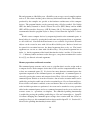
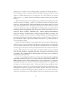
either over the Local Area Network (LAN) or the internet. The clients are platform independent and can be run on laptops, desktop computers or cluster nodes as illustrated
by figure 3.1.
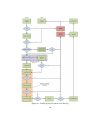
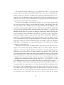
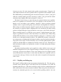
The grid process flow can be divided into three tiers: the end-user tier, the management tier and the computation tier. The process flow involving the three tiers is
shown in figure 3.2. An embarrassingly parallel problem implemented by the end-user
is called a project. Every project uses one or more bundles containing data or compiled executables of the worker code, e.g. an OpenCL application, that are created and
uploaded to the grid server by the end-user. The implementation of OpenCL worker
code is discussed in detail in chapter 6.2. The bundles are created using the Grid Management Kit (GMK) either directly or indirectly. The grid can be managed indirectly
through the Parallel Each (PEACH) [4, p.15] function that takes only a minimal set
of input parameters and manages the grid resources on behalf of the end-user. In the
9
Figure 3.1: Techila Grid infrastructure [3].
case of OpenCL applications the PEACH function does not however provide the level
of configurability needed to overcome the constraints presented in chapter 4, but by
managing the resources explicitly through local control code the constraints can be
overcome. Section 6.1 discussed the different aspects that have to be considered while
implementing the local control code for an OpenCL application.
Figure 3.2: Techila Grid process flow [4].
The management tier consists of the the grid server, the function of which is to
manage the projects, workers and bundles. When a project is created the grid server
splits the project into parallel tasks called jobs and distributes them to workers in the
grid. The number of jobs is defined by the end-user when the project is created. Every
10
project has an executor bundle that contains the worker code to be executed on the
workers. The executor bundle can be defined by the end-user to require resources from
other bundles, e.g. files from a data bundle. If the bundles required by a project are not
available locally the worker will download the required bundles from the grid server.
In cases where the bundle is large point-to-point transmissions can be used to distribute
the bundle to all the workers needing it. Every bundle created by the end-user is stored
on the grid server.
The management tier and the computational tier consisting of the workers are never
directly exposed to a regular end-user. The grid server has however a graphical user
interface (GUI) that can be accessed with a web browser. A regular end-user may
view information about the grid e.g. his projects, bundles and grid client statistics. An
administrator can configure the grid server and grid client settings through the GUI.
Among the things an administrator can do is to assign client features and create client
groups. The benefits of the two functionalities are discussed in section 4.3.
3.2
OpenCL architecture
In this section the OpenCL architecture is presented in terms of the abstract models
defined in the OpenCL specification [5]. The OpenCL specification defines four different models: the platform model, the memory model, the execution model and the
programming model. It is important to understand these models before writing worker
code that uses OpenCL.
3.2.1
Platform model
An OpenCL platform consists of a host and one or more compute devices [5]. An
OpenCL application consists of two distinct parts: the host code and the kernel. The
host code is run on a host device, e.g. a CPU, and it manages the compute devices and
resources needed to execute kernels. The host device may also function as a OpenCL
compute device. A function written for a compute device, e.g. an accelerator, a CPU or
a GPU, is called a kernel. The OpenCL application must explicitly define the number
and type of OpenCL compute devices to be used. The GPU is better suited for data
parallel problems than the CPU, which is well suited for task parallelism. The concepts
of data parallel and task parallel computation are explained in section 3.2.4.
11
Each compute device is comprised of several compute units and each OpenCL
compute unit contains a collection of processing elements. When discussing CPUs the
compute units are commonly known as cores. In Nvidia GPUs the compute units are
called Streaming Multiprocessors and the processing elements are called CUDA cores
[2]. In AMD GPUs the compute units were previously called SIMD Engines. A SIMD
� 5 processing elements each [10].
engine is comprised of Stream Cores that contain
�
��
Figure 3.3: OpenCL platform model [5].
��
The OpenCL standard has different versions and this has to be taken into consid-�
eration when writing portable code. The runtime and hardware may provide support
��
for different versions of the OpenCL standard and as such the programmer must check
�
that
the OpenCL platform version, compute device version and compute device lan��
��
guage
version are adequate. The platform version is the version supported by the
��
OpenCL runtime on the host, the compute device version describes the capabilities
��
of� the compute devices’ hardware and the compute device language version informs
��
the
programmer which version of the API he can use. The compute device language
��
version
cannot be less than the compute device version, but may be greater than the
��
�
compute
device version if the language features of the newer version are supported by
��
the card through extensions of an older version. The compute device language version
��
cannot
be queried in OpenCL version 1.0.
��
��
Every version of the OpenCL API has two profiles, the full profile and the embed��
ded
� profile. The embedded profile is a subset of the full profile and intended only for
��
portable
devices.
��
��
12
�
��
��
��
��
��
3.2.2
Execution model
Every OpenCL application has to define a context that contains at least one command
queue for every compute device being used [5]. A command queue is used to enqueue
memory operations, kernel execution commands and synchronization commands to
a compute device. The commands enqueued can be performed in-order or out-oforder. If more than one command queue is tied to a compute device the commands are
multiplexed between the queues.
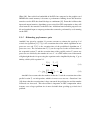
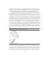
Figure 3.4: Example of a two dimensional index space [5].
A thread executing a kernel function is called a work-item. All work-items belong
to an N dimensional index space (NDRange), where N is either one, two or three,
that models the problem domain. When combined with the parallelism of the grid,
one can effectively compute four-dimensional embarrassingly parallel problems. The
NDRange is evenly divided into work-groups. A workgroup is a group of work-items
that are assigned to the same compute unit. The work-group size S can either be defined
explicitly by the programmer or be left to the OpenCL runtime to decide. If the workgroup size is defined explicitly the global index space has to be evenly divided by the
workgroup size, as shown by figure 3.4 where the two dimensional NDRange of size
13
Gx × Gy is evenly divided by workgroups of size Sx × Sy .
gx = wx ∗ Sx + sx
(3.1)
gy = wy ∗ Sy + sy
(3.2)
gz = wz ∗ Sz + sz
(3.3)
Every work-item in the NDRange can be uniquely identified by its global id, which
is the work-item’s coordinates in the NDRange. In addition every work-group is assigned a work-group id and every work-item within the work-group a local id. The
relation between the global IDs (gx , gy , gz ), the workgroup IDs (wx , wy , wz ) and the
local IDs (sx , sy , sz ) are shown by equations 3.1, 3.2 and 3.3. The global-, local- and
work-group IDs are made available to the work-item during kernel execution through
OpenCL C function calls.
3.2.3
Memory model
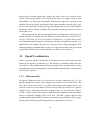
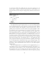
The memory model has a hierarchical structure, where the memory is defined to be
either global, local, constant or private [5]. Figure 3.5 shows the memory model of
an OpenCL compute device. The global memory can be written and read by both the
host device and the compute device, and memory objects can be allocated in either the
host devices’ memory space or the compute devices’ memory space. Memory objects
allocated in local memory however, that is usually located on-chip, is accessible only to
work-items belonging to the same work-group. The private memory space consisting
of registers is accessible only to the work-item that has allocated the registers. The
private memory space is by default used for scalar objects defined within a kernel.
Non-scalar memory objects are by default stored in the global memory space. Constant
memory is similar to global memory but it cannot be written by the compute device.
The local and private memory cannot be accessed by the host device, but local memory
can be statically allocated through kernel arguments.
All memory used by kernels has to managed explicitly in OpenCL. Transferring
data between host memory and device memory can be done explicitly or implicitly by
mapping a compute device memory buffer to the host’s addresspace. OpenCL memory
operations can be blocking or non-blocking. OpenCL uses a relaxed memory consistency. This means that the programmer has to ensure that all necessary memory oper14
Figure 3.5: OpenCL memory model [5].
ations have completed in order to avoid write after read and read after write hazards.
Data hazards are avoided by explicitly defining synchronization points within kernels
and command queues. No built-in mechanism exists however for synchronizing workgroups with each other.
3.2.4
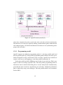
Programming model
OpenCL supports two different programming models, i.e the data parallel model and
the task parallel model [5]. Data parallel programming model utilizes the index spaces
defined in OpenCL to map a work-item to some set of data. OpenCL does not however
require a strict one to one mapping as some data parallel frameworks do.
In the task parallel model the NDRange consist only of one work-item. This is analogous to that of executing sequential code. The task parallel programming model is
intended to draw its benefits from being able to execute many kernels simultaneously,
given that the tasks do not have dependencies on each other. Additional performance
gain is achieved by using vector datatypes. The task parallel model is not recommended for GPUs.
15
4 G RID CLIENT REQUIREMENTS AND
SERVER CONFIGURATION
This chapter discusses the general hardware and software requirements placed upon a
grid worker for it to be able to run OpenCL applications. It is assumed that the Techila
Grid worker is a regular x86 based computer with one or more graphics cards and a
console. The last section of this chapter is devoted to the configuration of the Techila
grid and to the enhancement of job allocation.
4.1
Hardware requirements
Currently OpenCL applications can be executed on any x86 based CPU with the the
Streaming Single Instruction, Multiple Data Extension 2 (SSE2) and a wide variety of
AMD and Nvidia GPUs [7]. OpenCL is supported by all 8000 series and newer Nvidia
Geforce graphics cards and the ATI Radeon 5000 and newer series dedicated graphics cards [17]. Beta support exists for the ATI Radeon 4000 series dedicated cards.
All Nvidia Tesla computing processors and AMD FireStream 9200-series computing
processors support OpenCL. An up-to-date list of Nvidia and AMD graphics cards
supporting OpenCL, including mobile and professional graphics card models, can be
found from [17] and [7].
All graphics cards capable of OpenCL computations do not necessarily provide
good performance compared to CPUs. This is particularly true when old graphics
cards are compared to CPUs sold today, e.g. an Nvidia Geforce 8400 GS GPU has
only one compute unit with 8 processing elements. While each compute unit in an
OpenCL capable AMD GPU contains the same amount of processing elements, i.e. 80
processing elements per compute unit, the same does not hold true for Nvidia GPUs
[10]. With the shift from the GT200 architecture used by most of the 200-series cards
to the Fermi architecture used by the 400 and 500 series cards the amount of processing
16
elements per compute unit was increased from eight to 32 [2]. Therefore one should
not compare Nvidia GPUs to each other based on the number of compute units. This
is well exemplified by comparing the Geforce 280 GTX to the Geforce 480 GTX, the
first having 30 compute units while the latter has only 14, but despite this the Geforce
480 GTX has twice the number of processing elements.
Some of the old generation GPUs may even lack hardware support for certain functionality. For instance double precision floating point arithmetic is supported only by
Nvidia graphics cards based on the Fermi or GT200 architecture [12]. If a Nvidia
GPU is lacking support for double precision floating point arithmetic the operations
are demoted to single precision arithmetic. All ATI Radeon HD graphics cards in the
4800 and 5800-series support double precision arithmetic through AMD’s proprietary
OpenCL extension.
Another aspect to consider when hardware is concerned is memory. A desktop or
laptop computer has commonly between 512 MB and 8 GB of DRAM while a typical graphics card has between 64 MB and 1.5 GB of DRAM, i.e. global memory in
OpenCL terms. If the OpenCL application has to process a great amount of data on a
dedicated graphics card with e.g. only 128 MB of DRAM the application will cause
a lot of traffic over the PCIe bus, which is not desirable in terms of performance. It
should be noted also that AMD only exposes 50% of the total DRAM in its OpenCL
implementation [18]. The limit can be manually overridden, but AMD does not guarantee full functionality if this is done. Graphics cards based on the Fermi architecture,
i.e. those having compute capability 2.0, have read-only L1 and L2 caches that are
used by the runtime to speed up private- and global memory reads. Every compute
unit in the Fermi architecture has 64kB on-chip memory that is divided between the
L1 cache and local memory. Two thirds of the memory size is used for local memory
and the rest for the L1 cache. The L2 cache is larger than the L1 cache and shared by
all compute units. The AMD GPUs have L1 and L2 caches but those are only used for
texture and constant data and provide no significant performance gain in GPU computing [10]. Non-Fermi Nvidia cards have also texture and constant caches. In some
circumstances better utilization of the GPU may be achieved by using Direct Memory
Access (DMA) transfers between host and device memory. DMA transfers are performed by independent hardware units on the GPU and allow simultaneous copying
and computation. Nvidia calls these hardware units copy engines and every graphics
card with compute capability 1.2 or higher has a copy engine and devices with com-
17
pute capability 2.0 or higher have two copy engines [15]. Each copy engine is able to
perform one DMA transfer at a time. The AMD OpenCL implementation is currently
not capable of performing DMA transfers.
Special computing processors such as the AMD FireStream and Nvidia Tesla processors are intended solely for GPU computation [19, 20]. These cards tend to have
greater amounts of DRAM and features that are not needed in desktop graphics cards
such as Error-Correcting Code (ECC) applied to on-chip memory and device memory.
For instance the AMD FireStream provides up to 2 Gb of DRAM and the Tesla 2000series cards provide up to 6 GB of DRAM.
4.2
Software requirements
A compiled OpenCL application will need the OpenCL runtime to execute on a grid
worker. The runtime consists of the OpenCL library and one or more OpenCL drivers.
The drivers are mostly vendor specific and provide support for a certain set of hardware. Nvidia has included its implementation of the OpenCL 1.0 runtime library in its
display driver package from release 190 onwards [8]. This means that every worker
with a CUDA capable graphics card and an up-to-date display driver has the capability to run OpenCL applications. At the moment of writing OpenCL 1.1 support is
available only through release candidate development drivers.
With the Catalyst 10.10 display driver AMD introduced the Accelerated Parallel
Processing Technology (APP) edition display driver package that includes the AMD
OpenCL runtime implementation. The APP edition display driver is currently only
available for Windows, but an APP edition of the Linux display driver package is
planned for year 2011 [21]. To run OpenCL applications on AMD graphics cards
under Linux the ATI Stream SDK, which also includes the OpenCL library and driver,
has to be installed. This applies also to Windows workers without the APP edition
display driver.
The Nvidia OpenCL driver supports only the vendor’s own lineup of graphics
cards, while the AMD OpenCL driver supports all x86 based CPU with SSE2 and
the company’s own lineup of graphics cards. Many implementations of the OpenCL
runtime may co-exist on a worker because of the Installable Client Driver (ICD)
model, which is used by both Nvidia and AMD OpenCL runtime implementations
[22]. In the ICD model an OpenCL driver registers its existence in a common location
18
Figure 4.1: The OpenCL runtime layout.
which is checked by all drivers using the ICD model. In Windows the OpenCL drivers
are registered under HKEY_LOCAL_MACHINE/SOFTWARE/Khronos/OpenCL/Vendors
by specifying a registry key with the driver library’s filename. In Linux the registration
is done by placing a file, with the file extension icd, under /etc/OpenCL/vendors containing the driver’s filename. The Nvidia display driver installer registers the OpenCL
driver automatically under Windows and Linux. The ATI Stream SDK registers the
AMD OpenCL client driver automatically under Windows, but under Linux an additional package has to be downloaded and extracted for the driver to become registered
[23]. If the different OpenCL drivers have been correctly installed, the preferred
OpenCL platform can be chosen using the clGetPlatformIDs OpenCL API call.
Techila Grid provides the option to manage runtime libraries by creating library
bundles that can be distributed to the workers in the grid [4]. The OpenCL runtime is
however dependent of the graphics card drivers installed on the worker, which makes
it poorly suited for this type of centralized model of library management. For instance
the OpenCL 1.1 driver supplied with ATI Stream SDK 2.2 requires Catalyst driver suite
19
version 10.9 in order to work correctly as the OpenCL driver depends on the Compute
Abstraction Layer (CAL) runtime embedded in the display driver package [7, 10].
Dependencies between the OpenCL runtime implementations and the display drivers
are not documented in detail by the vendors and therefore it cannot be guaranteed that
runtimes packaged in library bundles will function correctly on all workers. Even if
the library bundles were used, local management would still be required for workers
with both AMD and Nvidia graphics cards because of the ICD model.
4.2.1
Operating system constraints
Both Nvidia and ATI provide their OpenCL runtime for Windows and Linux operating
systems, but due to certain implementation decisions a Techila Grid worker cannot
run OpenCL applications on all the operating systems listed as supported by Nvidia or
AMD. Table 4.1 shows a list of operating systems and the hardware resources that are
accessible by the worker through the vendor specific OpenCL drivers.
Operating system
Fedora 13
openSUSE 11.2
Ubuntu 10.04
Red Hat Enterprise Linux 5.5
SUSE Linux Enterprise Desktop 11 SP1
Windows 7
Windows Vista
Windows XP
Windows Server 2003, 2008
Mac OS X 10.6
AMD GPU
Yes2
Yes
Yes
Yes
Yes2
No
No
Yes1
No2
Yes
Nvidia GPU
Yes
Yes
Yes
Yes
Yes
No
No
Yes
Yes
Yes
x86 CPU
Yes2
Yes
Yes
Yes
Yes2
Yes
Yes
Yes1
Yes2
Yes
Table 4.1: Hardware accessible under different operating systems [7, 8].
Under Windows the Techila Grid Client runs as a service under a dedicated user
account. When OpenCL support is considered this becomes a limiting factor on some
versions of Windows. Microsoft changed the way regular processes and services are
handled from Windows Vista and Windows Server 2008 onwards [24]. In operating
systems until Windows XP and Windows Server 2003 all services run in the same
1
2
SP3 required for the 32-bit operating system. Beta support for 64-bit operating system requires SP2
Not officially supported
20
session as the first user that logs on to the console. In an effort to improve security
Microsoft decided to move the services to a separate non-interactive session. This
change is commonly know as session 0 isolation. The aim of this change was to make it
more difficult for malicious software to exploit vulnerabilities in services that run with
higher privileges. The services running in session 0 are assumed to be non-interactive
and have therefore no access to the display driver. From this it follows that no OpenCL
application utilizing the GPU can be run by the worker.
The only exception to the previously mentioned rule is the Nvidia Tesla series
GPU computational cards [25]. The Tesla display driver has a mode called Tesla Compute Cluster (TCC). When this mode is engaged processes in session 0 can access the
graphics hardware for computational purposes on Windows operating systems otherwise affected by session 0 isolation. The TCC mode does not support drawing of 2D or
3D graphics, i.e. the graphics card cannot be attached to a display if the TCC mode has
been engaged. All non-Tesla Nvidia graphics cards will be demoted to VGA-adapters
when TCC-mode is engaged. The driver supporting TCC-mode is available for all
Windows operating systems listed in table 4.1.
Windows XP and newer Windows operating systems monitor the responsiveness
of the graphics driver. If the graphics driver does not respond within a certain time
limit Windows considers the driver unresponsive and tries to reset the display driver
and graphics hardware. In Windows XP the graphics card is monitored by a watchdog timer and the default timeout is 2 seconds [23]. In Windows Vista and Windows
7 the feature is called Timeout Detection and Recovery (TDR) [26] and the timeout
is 5 seconds. When performing OpenCL calculations on the GPU these time limits
may be exceeded by computationally intensive kernels which will cause the display
driver to be reset. When a display driver is reset the kernel is forced to interrupt
without storing any results. From a computational point of view this is undesired
behavior and therefore these features should be disabled. The TDR functionality
can be disabled by creating REG_DWORD TdrLevel in HKEY_LOCAL_MACHINE/
SYSTEM/CurrentControlSet/Control/GraphicsDrivers with value 0 in the registry. To
disable the Windows XP display driver watchdog timer the REG_DWORD DisableBugCheck with value 1 has to be inserted at HKEY_LOCAL_MACHINE/SYSTEM/
CurrentControlSet/Control/Watchdog/Display in the registry. Workers with ATI graphics cards should also disable VPU Recovery as explained in [23]. Microsoft advises
against disabling these features.
21
Similar restrictions as those caused by session 0 isolation exist under Linux for the
AMD OpenCL implementation. CAL accesses the graphics card hardware through
the existing interfaces of the X server [27]. The grid client runs as a process under a
dedicated user account that does not have an X server running. Access to the console’s
X session can however be gained by modifying the X server access control list and
allowing the grid user to read and write to the graphics card device nodes. One way
of achieving this is to add the following two lines to the XDM or GDM initialization
scripts that are run as root. The XDM setup script, located at etc/X11/xdm/Xsetup,
is used by both the KDE and X window managers. The GDM initialization script is
located at /etc/gdm/Init/Default. In addition to these two settings the environmental
variable DISPLAY with value :0 has to added to the run environment.
chmod a+rw / dev / a t i / c a r d ∗
x h o s t +LOCAL :
The Nividia OpenCL runtime does not require that the X server settings are modified, but the grid client user account has to have read and write access to the device
nodes. Similarly to the AMD systems access rights may be granted through the XDM
or GDM initialization scripts.
chmod a+rw / dev / n v i d i a ∗
4.3
Grid server configuration
The grid workers can be coarsely divide into those capable of OpenCL computations
and those not capable of OpenCL computations. This sort of division is a good starting point with regard to job allocation but not necessarily the best when performance
is concerned. By default the grid server has no knowledge what kind of graphics hardware or which runtime components a worker has. If this information is not registered
in any way jobs will be allocated to workers without runtime components or hardware
that supports GPU computation. If a job is allocated to a worker without OpenCL
support the worker code will fail to execute and the grid will reallocate the job. Many
errors caused by lacking OpenCL support can cause a project to fail if 90% of the jobs
belonging to the project fail once or 10% of the jobs fail twice. The probability of
project failure can however be eliminated by assigning features to the grid clients.
The first step in enhancing the job allocation would be to form a client group of
22
OpenCL capable workers, i.e. workers with the runtime components and GPUs supporting OpenCL. Every worker would then be guaranteed to execute at least some part
of the OpenCL application assigned to them. OpenCL is an evolving standard and
as such every worker is not guaranteed to support the same set of OpenCL features,
e.g. sub-buffers are supported by OpenCL 1.1 but not by OpenCL 1.0. These differences can be taken into account by assigning the clients a feature that tells the OpenCL
runtime version installed on that worker. Beside the core functionality every OpenCL
version has a set of optional extensions. The OpenCL application can query these at
runtime, but a better option would be to store the supported extensions as features. This
way an OpenCL project using e.g. 64-bit atomic operations could be directly allocated
to compatible workers.
In addition to the software requirements a set of hardware features can be assigned
to clients. Nvidia defines a value called compute capability for every Nvidia graphics
card supporting GPU computation. This value has a major number followed by a
decimal point and a one digit minor number. The compute capability value is used to
describe the characteristics of the graphics hardware and is the same for all graphics
cards based on the same architecture. The compute capability can be queried during
runtime using Nvidia’s proprietary OpenCL extension cl_nv_device_attribute_query.
AMD does not have any similar value that describes the hardware capabilities of their
graphics cards. Instead the AMD graphics cards can be divided according to their
hardware architecture. All dedicated graphics cards with the same leading number
in their model name have the same hardware characteristics. Knowing the hardware
architecture could be used to optimize the worker code or to simply discard workers
with graphics cards that perform poorly in some specific task. An example of such a
situation would be to discard Nvidia GPUs with compute capability 1.0 or 1.1 when
the OpenCL kernel exhibits unaligned memory access patterns. Graphics cards with
the mentioned compute capabilities cannot detect unordered accesses to a section of
memory and may in the worst case cause as many fetch operations on the same section
of memory as there are threads in the half-warp [2].
23
5 L IBRARIES AND APPLICATIONS
UTILIZING GPU COMPUTATION
OpenCL is a young standard and as such there are few evolved tools that are based on
it. When compared to CUDA, the lack of vendor specific optimized libraries currently
limits the adoption of OpenCL in scientific applications. Optimized CUDA libraries
exists for fast Fourier transforms (FFT), linear algebra routines, sparse matrix routines
and random number generation. While these kinds of libraries can be expected for
OpenCL in the future the current offering is scarce. On a side note it should however be
observed that every grid client with an Nvidia GPU capable of OpenCL computations
can be made capable of executing applications and libraries based on C for CUDA.
This chapter will primarily focus on libraries and application that use OpenCL, but
also discusses some CUDA based products.
5.1
Linear algebra libraries
The Vienna Computing Library (ViennaCL) is a Basic Linear Algebra (BLAS) library
OpenCL implementation developed by the Institute for Microelectronics of the Vienna
University of Technology [28]. Currently ViennaCL supports level one and two BLAS
functions, i.e. vector-vector operations and matrix-vector operations, in single and
double precision, if supported by hardware. Level three operations, i.e. matrix-matrix
operations, will be added in future releases. ViennaCL’s primary focus is on iterative
algorithms and as such ViennaCL provides interfaces for conjugate gradient, stabilized
biconjugate gradient and generalized minimum residual iterative methods. ViennaCL
is a header library that incorporates the OpenCL C kernel source codes inline. A
compiled application using the ViennaCL library can therefore be executed on any
grid client with the OpenCL runtime. If the current functionality of ViennaCL is not
sufficient the user can implement his own OpenCL kernels that extend the ViennaCL
24
library. Section 5 of the ViennaCL user manual [28] provides instructions on how to
extend the library.
CUBLAS is a BLAS library utilizing Nvidia GPUs [29]. It is included in the
CUDA Toolkit that is available for Linux, Windows and OS X operating systems.
CUBLAS uses the CUDA runtime but does not require the end-user to directly interact
with the runtime. The CUBLAS library provides all three levels of BLAS functions
through its own API. CUBLAS supports single precision floating point arithmetic and
also double precision arithmetic if the hardware is compatible. Using the CUBLAS library in the grid will require the creation of library bundles that contain the CUBLAS
libary file, e.g. cublas.so, against which the application is linked at compilation. The
CUDA driver is installed with the display drivers but the CUDA runtime library, e.g.
cudart.so, has to be made available through a library bundle. It should be noted however that the CUBLAS, CUDA runtime, and CUDA driver libraries have to be of the
same generation to ensure full compatibility, i.e. the workers’ display drivers should
be of the version specified in the CUDA toolkit release notes and the CUDA runtime
and CUBLAS libraries should be from the same CUDA toolkit release.
CULA is a commercial third party Linear Algebra Package (LAPACK) implementation from EM Photonics Inc [30]. The basic version of CULA is available free of
charge but it provides only single precision accuracy. CULA provides two C language
interfaces for new developers, a standard interface that uses the host memory for data
storage and a device interface that uses the graphics card’s DRAM for storage. The
standard interface is aimed at those end-users not familiar with GPU computation.
When the standard interface is used all transfers between host and device memory are
hidden by CULA. An interface called bridge is provided, in addition to the standard
and device interfaces. The bridge interface is intended to ease the transition from popular CPU based LAPACK libraries to CULA by providing matching function names
and signatures. The bridge interface is built on top of the standard interface. CULA is
provided as a dynamic library that uses the CUDA runtime library and the CUBLAS
library. All the before mentioned libraries are provided with the install packages. Similarly to CUBLAS these libraries have to be made available to the worker executing a
CULA application. All the CULA specific information needed for creating a Techila
grid library bundle is made available through the CULA programmer’s guide in the
installation package. The CULA install package is available for Windows, Linux and
OS X.
25
5.2
Matlab integration
The Techila Grid uses the Matlab compiler and the Matlab compiler runtime to execute
Matlab source code on the grid. The Matlab source code is compiled by the end-user
with the Matlab compiler. The binary is then packaged in a binary bundle that is
defined to have a dependency on the Matlab compiler runtime, and uploaded to the
grid server. The Matlab compiler runtime is made available to grid clients through a
library bundle. When a job that uses the Matlab binary bundle is received by a grid
client it will notice the dependency and use the Matlab compiler runtime library bundle
to execute the binary. In general there are three ways to utilize GPU computation in
Matlab. The first way is to use the Matlab 2010b Parallel Computing Toolbox, the
second way is to use the Matlab Executable (MEX) external interface and the third
way is to use third party add-ons.
The built-in GPU support in the Matlab 2010b Parallel Computing Toolbox is based
on the CUDA runtime, but restricted in functionality [31]. Matlab provides function
calls that utilize the CUDA FFT library but otherwise only the most basic built-in
Matlab functions can be directly used through Matlab’s GPUArray interface. The builtin GPU computing interfaces are not supported by the Matlab compiler, which hinders
their usage in Techila Grid.
The low level approach is to use MEX external interface functions that utilize
OpenCL. ViennaCL has a distribution where the MEX interfaces are already implemented [32]. The only thing that remains for the end-user is to compile the MEX
files and use them in a Matlab application. At this time the developers of ViennaCL
recommend using their solvers over the ones in Matlab only for systems with many
unknowns that require over 20 iterations to converge. The ViennaCL library uses row
major order for its internal matrices, while Matlab uses column major order. This
forces ViennaCL to transform the input and output data which causes a performance
penalty. Additionally Matlab uses signed integers while ViennaCL uses unsigned integers. It is also possible to implement custom MEX functions that utilize OpenCL.
Matlab Central [33] provides a good tutorial for writing MEX-functions in the C language. OpenCL code incorporated in a MEX-function does not differ from the program
flow shown in figure 6.2. A few aspects should however be kept in mind. All input and
output data should go through the MEX interface. As Matlab uses by default double
precision floating point values the host code should check that the GPU being used
supports double precision arithmetic and if not convert the values to single precision.
26
To enhance the portability of the MEX function the OpenCL C kernel code should be
written inline.
Jacket is a third party commercial add-on to Matlab developed by AccelerEyes
[34]. Jacket is built on top of the MEX interface that is used to interact with CUDA
based GPU libraries, e.g. the CUBLAS and CUFFT library. AccelerEyes provides a
product called Jacket Matlab Compiler (JMC) that uses the Matlab compiler in combination with the Jacket engine to produce binaries that can be deployed independently.
The Jacket Matlab compiler binaries are executed with the Matlab compiler runtime
and do not therefore differ from any other Matlab binary that is executed on the grid.
To create non-expiring Jacket Matlab applications that can be run on the grid the base
license and a Jacket Matlab compiler license are required. Double precision LAPACK
is available at additional cost. A grid client deploying a Jacket Matlab compiler binary
does not require a license.
27
6 I MPLEMENTING A T ECHILA G RID
O PEN CL APPLICATION
This chapter uses a top-down approach to describe how an OpenCL application and
the local control code should be implemented so that the OpenCL application can be
executed on the grid. Please read chapter 3 before reading this chapter.
6.1
Local control code
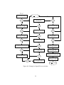
The Techila local control code differs only little from regular projects not performing
OpenCL GPU computation. The local control code can be implemented in any of the
supported programming languages, e.g. Java, C, Python, etc. The local control code
flow is depicted in figure 6.1. The programming language specific syntax is explained
in [6].
In the simplest case the grid is initialized, a session is opened, a binary bundle is
created, the bundle is uploaded and a project using the bundle is created [6]. There are
however a few key aspects that have to be taken into account when creating the binary
bundle for an OpenCL application if the OpenCL C source code is stored in a separate
source file instead of being embedded in the OpenCL application binary. If a separate
source file is used this file has to be specified as an internal resource and included in
the binary bundle’s file list. In addition the source file has to be copied to the execution
directory at runtime. This can be done with the bundle parameter copy.
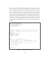
Workers that use the ATI Stream Software Development Kit (SDK) libraries have
to be instructed where to look for the library files because the SDK libraries are not
installed to any of the default system library locations. A linux worker can locate
the OpenCL libraries required at runtime if the LD_LIBRARY_PATH environmental
variable is set to point to the folder with the libOpenCL.so file. The simplest way to
export the LD_LIBRARY_PATH environmental variable to the workers runtime
28
Techila Developer's Guide Copyright © 2010 Techila Technologies Ltd. P a g e | 24 Figure 6.1: Techila grid local control code flow [6].
29
environment is by using the bundle parameter environment. Using an absolute path
as value for the environmental variable would however require that the SDK has been
installed to the same path on every worker. This restriction can be bypassed by storing
the OpenCL library path as a client feature and using the %A macro when specifying
the value of LD_LIBRARY_PATH. A Windows worker will find the necessary AMD
library files as long as the grid is not instructed to override the local system variables.
If the grid has Linux workers with AMD GPUs the DISPLAY variable with value :0
has to be exported to the execution environment so that any requests from the OpenCL
runtime are directed to the correct X server. Section 4.2.1 describes in more detail
about the AMD X session constraints. Nvidia and AMD provide both 32-bit and 64bit OpenCL drivers in their display driver and SDK packages for 64-bit operating systems. Therefore there is no need to add operating system constraints to a binary bundle
containing a 32-bit OpenCL application binary. When dealing with 64-bit OpenCl application binaries, the executable should be constrained to 64-bit operating systems
only using the processor parameter.
One may either choose to include possible input data files in the binary bundle or
create a separate data bundle. When all bundles have been created, a binary bundle
is selected to be used and a project is created. Current limitations in GPU hardware
allow for only one OpenCL context to be active at the GPU at any given moment
[12]. When several applications are using the same GPU the GPU’s resources are
time sliced. The time slicing is done by context switching. If many computationally
intensive jobs are allocated to the same worker and they all use the same OpenCL
compute device, there is a risk that the compute device becomes overloaded. If a GPU
is under heavy computational load all graphics drawing might become sluggish at the
console. This applies especially to cards with low performance and is not desirable.
The number of jobs utilizing the same GPU can be restricted by setting the project
parameter techila_multithreading to true. This will ensure that only one job will be
running at each worker assigned to the project.
To avoid unnecessary job allocations to workers without OpenCL hardware and
runtime components it is recommended that the workers are assigned features or divided into groups as explained by section 4.3. When this approach is used the local
management code has to tell the grid server which worker group is to be used for the
project and which features are required from the workers. The client group is selected
by giving the client group name as value to parameter techila_client_group when the
30
project is created. Any features required by the OpenCL application can be enforced
with the techila_client_features project parameter. The features can be specified to be
equal, greater or equal , less than or equal to a value or any value. If some feature is not
enforced by the local management code the worker code has to check that this feature is
supported by the platform and the compute device at runtime using clGetPlatformInfo
and clGetDeviceInfo OpenCL API calls.
6.2
OpenCL worker code
This chapter will describe the process of writing a cross-platform compatible OpenCL
application. An OpenCL application can be divided into two components the host code
and the kernel code. The steps in implementing the OpenCL host code are explained
with the help of a flow graph. The OpenCL API and OpenCL C syntax is not discussed
in detail as it is well documented in [5]. It is recommended that the OpenCL application
is developed, tested and proven functional locally before running it on the grid. Before
reading further it is strongly recommended that the reader has read chapter 3.2 and
understood the key concepts of the OpenCL architecture presented in that chapter.
When developing OpenCL applications on a Windows or Linux computer a software development kit such as the NVIDIA GPU Computing SDK or the ATI Stream
SDK has to be installed. Note that the NVIDIA GPU Computing SDK will require
the development version of the ForceWare display driver. Besides containing all the
necessary library and header files the SDKs contain sample programs, utility libraries
and vendor specific documentation. If the development is done in OS X the development tools package has to be installed. On Unix platforms the OpenCL host code can
be compiled with the gcc compiler. Under Linux the OpenCL library flag -lOpenCL
has to be passed to the gcc compiler and in OS X the the compiler has to be instructed to use the OpenCL framework by passing the flag -framework OpenCL to the gcc
compiler. If the application development is done in Windows the compilation can be
performed with Microsoft Visual Studio. Detailed instructions how to do this can be
found from the programming guides [10] and [2].
6.2.1
OpenCL host code
The purpose of the host codes is to manage the compute devices and the resources they
have. This is achieved through the OpenCL API. Experimental C++ bindings exist
31
for the OpenCL API, but this section will refer to the C language API defined by the
OpenCL specification. To use the OpenCL API calls under Windows or Linux one
must include the header file CL/cl.h. The OS X operating system uses a slightly different path, OpenCL/cl.h, for the same header file. The include command can be made
portable across operating systems by using preprocessor instructions. The OpenCL
API is logically divided into two parts, the platform layer and the runtime layer. The
platform layer contains commands for discovering OpenCL platforms and compute
devices, while the runtime layer has commands for managing kernel functions, queues
and memory objects. The platform layer host code varies seldom, while the structure of
the runtime layer host code may vary greatly from application to application depending on the problem being solved. The bare minimum of objects needed by an simple
OpenCL application is a platform, a context, a device, a command queue, a program,
a kernel and and one or more memory buffers as shown by the sample program flow in
figure 6.2.
All OpenCL 1.1 API calls except clSetKernelArg are thread safe and in OpenCL
1.0 all API calls except those beginning with clEnqueue are thread safe [5, 35]. Every
OpenCL API call returns an error code if the operation in question fails. The possibility
that errors occur should always be taken into account by the host code as the hardware
might vary greatly from client to client.
Creating a context
The first step in writing the host code is to query the platform ID. A host system might
have more than one OpenCL implementation, i.e OpenCL drivers, installed that are
all uniquely identified by a platform ID [5]. A common approach to select the preferred platform is to use command clGetPlatformIDs to query the number of platforms
available, allocate the space needed for the platforms available and then use clGetPlatformIDs a second time to get the actual platform IDs from which the preferred platform
can be selected. In figure 6.2 the default platform’s ID is queried directly. Additional
information about the platform such as platform name, vendor, OpenCL version and
OpenCL extensions can be queried using the command clGetPlatformInfo.
32
Figure 6.2: Example of OpenCL host code flow.
33
The second step is to query the compute devices associated with the platform ID of
step one using the clGetDeviceIDs API call. The second argument in clGetDeviceIDs
is used to specify what type of OpenCL compute devices are desired. The different
types are all, accelerator, CPU, default and GPU. The number of devices associated
with a platform can be queried in a similar manner as with the platforms. The API
call clGetDeviceInfo can be used to query a wide range of over 50 device properties, a
complete list of which can be found in section 4.2 of [5]. The device parameters most
commonly needed are device type, supported extensions, maximum work-group size,
maximum work-group dimensions, the greatest allowed buffer size, global memory
size, global memory cache size, local memory size and the device OpenCL C version.
Every OpenCL runtime layer object is related to a context, either directly or indirectly through some other object. The context can be seen as a container for all objects
created by the runtime layer. A platform and the devices belonging to it may be associated with more than one context, but commonly an OpenCL application has only
one context. Runtime layer objects cannot be shared by different contexts. A context
may be created in two different ways, either by passing one or more compute device
IDs as arguments to clCreateContext or by passing the desired compute device type to
clCreateContextFromType. If the latter command is used the platform used is OpenCL
implementation defined. In that case the platform and devices associated with the context can be queried using clGetContextInfo and clGetDeviceInfo. It should be noted
that clCreateContextFromType is not guaranteed to return all available devices of the
requested type, hence it is preferable to use clCreateContext.
Creating memory buffers
Because of the hierarchical memory structure of OpenCL special memory objects and
operations are needed for reading, writing and copying data. In OpenCL arrays and
user defined datatypes have to be allocated in continuous sections of memory. To force
this behavior OpenCL has memory buffers. A memory buffer of desired size is allocated in global memory with clCreateBuffer [5]. The memory access of the kernel
functions can be restricted by specifying the buffer as read only or write only. By
default the buffer is allocated in device memory, but if needed the buffer can be allocated in host memory. A buffer can be allocated in host memory by passing a pointer
to a memory segment and the host pointer flag to clCreateBuffer. The clCreateBuffer
command can also be instructed to initialize the memory buffer with data from a host
34
pointer. If this functionality is used there is no need to copy the host pointer data explicitly to the buffer by invoking clEnqueueWriteBuffer as explained in section 6.2.1.
If the application being implemented is memory intensive, care should be taken that
the global memory size and greatest allowed buffer size limits are not exceeded. These
limits can be queried using clGetDeviceInfo. It should also be noted that the amount
of graphics card DRAM may vary greatly from compute device to compute device. If
the limits are exceeded the memory allocation will fail.
Allocating buffers in host accessible memory is desirable when the data is to be
processed by the CPU. Using host memory with the GPU as compute device is not
desirable as the PCIe bus limits the memory bandwidth considerably compared to the
GPUs DRAM bandwidth. With Nvidia graphics cards higher transfer speeds bandwidth over the PCIe bus can be achieved using pinned memory, also known as page
locked memory. This feature requires the usage of a specific implementation pattern
described in section 3.1 of [15].
Compiling OpenCL kernels
A task that is executed in parallel is called a kernel and many kernels form a program
[5]. The term program should not be confused with the term OpenCL application. A
program is an object and an OpenCL application is the whole application. An OpenCL
program object is created from a C string containing the OpenCL C source code or
from a precompiled binary. The OpenCL C source code can be stored as a string in the
host code or as a separate source file that is read by the host code. The Nvidia shrUtils
and AMD SDKUtils utility libraries in the vendor SDKs include routines for reading
the OpenCL C source code file to host memory. A common convention is to store the
OpenCL C source code in a file with the cl file extension. The process of writing a
kernel is described in section 6.2.2. The program object is created by invoking the
clCreateProgramWithSource with the source code string as a parameter, in a similar
way the program object may be created from a precompiled binary by invoking the
clCreateProgramWithBinary. The binary codes and device IDs passed as argument to
clCreateProgramWithBinary must match the hardware architecture or the API call will
fail.
OpenCL uses Just In Time (JIT) compilation [11]. The OpenCL C compiler is part
of the OpenCL driver and cannot as such be invoked offline as traditional compilers.
The source code is compiled for the desired compute devices by passing the device
35
IDs and program to clBuildProgram. clBuildProgram accepts a set of compiler options
such as -I, the relative include path to directory with kernel header files. The binaries
produced by the compiler are specific to the hardware architectures of the compute
devices. The program binaries can be extracted using clGetProgramInfo. For Nvidia
GPUs the binary returned is Parallel Thread Execution (PTX) binary and for AMD
GPUs ATI Intermediate Language (ATI IL) binary [10, 2]. For better portability it is
recommended that the program object is always created from the OpenCL C source
code.
Work is sent to compute devices by enqueueing kernels to the command queue. A
kernel object is created by passing the kernel name and program object as arguments
to clCreateKernel. Note that the kernel name is case sensitive. If preferred all kernel
objects can be created at once with clCreateKernelsInProgram. Before a kernel can
be queued for execution however, the kernel arguments have to be set. The kernel
arguments are set one at a time with clSetKernelArgs. Every kernel argument has an
index, i.e. the first argument of the kernel function has index 0 and the N th has index
N − 1. Memory buffers and most scalar data types, except those mentioned in section
6.8 of [5], are allowed as kernel arguments.
Memory operations and kernel execution
The command queue structure can be seen as a pipeline that is used to assign work to
a compute device. Each compute device that is to be used for computation has to have
at least one command queue [5]. If a device has more than one command queue the
operations enqueued to the command queues are multiplexed. A command queue is
created by passing the context and compute device ID to clCreateCommandQueue. A
command queue defaults to in-order-execution. Out-of-order execution mode can be
enabled by passing the enable out-of-order execution flag to clCreateCommandQueue.
If out-of-order execution is enabled, events and barriers have to be used to control the
order in which operations are performed. An event can be attached to every operation
added to the command queue and every command enqueued can be set to wait for one
or more events, i.e. operations, to complete. The embedded profiling functionality
is enabled by passing the profiling enable flag to clCreateCommandQueue. OpenCL
1.0 allows changing the command queue settings after creation with the clSetCommandQueueProperty, this command has been deprecated in OpenCL 1.1. Section 6.2.3
discusses the profiling functionality in more detail.
36
All commands starting with clEnqueue are asynchronous calls, i.e. they will return
control to the host program immediately. The memory read, write and mapping operations can however be made synchronous by setting the blocking parameter to true.
Another way of synchronizing the host program thread with the command queue is by
using the clFinish call. clFinish will block the host program thread until all commands
enqueue before clFinish have been completed.
In a trivial program flow, as that shown in figure 6.2, one or more memory buffers have been created. Data is copied from host memory to the buffers with clEnqueueWriteBuffer and from buffer to host memory with clEnqueueReadBuffer. Data
can also be copied from one buffer to another with clEnqueueCopyBuffer. Sometimes
it is necessary to modify the buffer data allocated in device memory, e.g. graphics card
DRAM, from the host code. Instead of reading the data from the buffer, modifying the
data and writing it back to the buffer, the buffer or a section of it may be mapped for
reading or writing to the host’s memory space with clEnqueueMapBuffer. The pointer
returned by clEnqueueMapBuffer to the mapped memory region can then be used to
access and modify the data in a traditional manner. The content of the memory buffer
mapped for writing is considered undefined until the memory segment is unmapped
with clEnqueueUnmapBuffer. A mapped buffer should not be written to from a kernel
or multiple command queues.
When the necessary input and output buffers have been created a kernel can be
enqueue for execution with clEnqueueNDRangeKernel or clEnqueueTask. The first
of these is used for data parallel kernels and requires as input the global work size
(NDRange), the local work size and dimensionality of the problem. The global work
size that naturally follows from some data structure might not always be evenly divided
by the workgroup size as required by the runtime. In these cases the global index space
is defined as greater than the index space of the data set and the differences in size
is handled with conditional statements in the kernel code. As of OpenCL 1.1 clEnqueueNDRangeKernel also accepts offset values that are added to the the global x, y
and z coordinates. This feature is particulary useful if the required global work size is
not supported by the compute device, as it allows for the problem to be split into smaller problems. The maximum global work size can be queried with clGetDeviceInfo.
For optimal usage of the GPU compute units the global work size should be a multiple
of the wavefront size or the warp size, i.e 64 or 32. If the local work-group size is of
no significance to the algorithm a null value may be given as input and the runtime
37
will select a suitable value. Every compute device has a maximum work-group size
that cannot be exceeded. The maximum size varies greatly from device to device, but
work-group sizes up to 256 are supported by all OpenCL capable AMD GPUs, Nvidia
GPUs and x86 CPUs. clEnqueueTask is used to enqueue task parallel kernels, i.e kernels with only one work-item. Concurrent kernel execution is currently supported only
by the Nvidia cards based upon the Fermi architecture and hence this form of parallelism is not applicable for GPU computing on a grid [12]. The OpenCL standard
specifies also a third type of kernel called native kernel, which is a regular function
written in C or C++. This type of kernel would not be compiled by the OpenCL compiler. A native kernel would be enqueued for execution by passing a function pointer
to clEnqueueNativeKernel, but currently native kernels can not be executed on AMD
or Nvidia GPUs [23, 36]. Native kernels are supported by x86 CPUs.
Cleanup
All objects created in the runtime layer should be released before the application exits.
The objects should be released in the reversed order that they have been created, i.e
kernels are released first and the context as last. Figure 6.2 shows the order in which
to release the objects.
6.2.2
OpenCL kernels
This subsection will shortly present the OpenCL C language and the different aspects
that should be taken into account when writing an OpenCL C kernel.
The OpenCL C language
The OpenCL C language is based on the ISO/IEC 9899:1999 standard, also known
as C99 [5]. The restrictions and capabilities of the OpenCL C language used to write
OpenCL kernels are defined by [5] and listed here under. Extended functionality is
provided by optional OpenCL extensions [5]. The shortcomings of the programming
language can mostly be overcome by alternative implementations.
OpenCL C core functionality not found in C99:
• 32-bit atomic operations
• Built-in vector datatypes
38
• Built-in vector functions
• Built-in geometric functions
C99 functionality not found in OpenCL C:
•
•
•
•
•
•
•
Recursion
File operations
Standard I/O operations
Function pointers
Bit-fields
Dynamic memory allocation
Support for double precision floating point operations
OpenCL C extended functionality not found in C99:
• 64-bit atomic operations
• Built-in double and half precision floating point vectors
• Half precision floating point support
OpenCL C does not support standard C libraries when using a GPU as compute
device [5]. The implication of this is that no file or standard I/O operations can be
carried out from the kernels running on a GPU and these have to be handled by the
host code. The concept of host code is explained in section 3.2.1. Another implication
of the missing C library support is that all string operations, such as string compare and
string concatenation, have to be implemented by the programmer as needed. OpenCL
1.0 lacks by default support for writing to pointers or arrays of datatypes less than 32bits, such as characters and short integers. Devices that support the byte addressable
store extension by Khronos are not however affected by this restriction. When taking
these two factors into consideration OpenCL 1.0 is not well suited for dealing with
strings. The byte addressable store extension was adopted as part of OpenCL 1.1.
The missing support for the C99 math library on the other hand is insignificant as
OpenCL C provides a better set of built-in functions than the standard C99 library. The
built-in math operations can be applied to scalars, built-in vector types or individual
components of a vector. Noteworthy groups of special functions are the atomic and
geometric functions. The atomic operations are guaranteed to operate on the shared
data one work-item at the time, essentially making the accesses sequential. OpenCL
1.1 has built-in support for 32-bit atomic integer operations, but atomic operations on
long integers are supported only through the 64-bit atomics extensions. OpenCL 1.0
39
supports 32- and 64-bit atomic operations only through extensions. The geometric
functions include routines for calculating dot products, cross products, vector lengths,
vector normals and distances between two points.
The most notable addition compared to standard C are the built-in vector datatypes
and the math operations supporting them. The OpenCL vector types are derived from
the standard C scalar datatypes and can have a length of 2, 3, 4, 8 or 16 elements,
e.g. uchar4, long8, float16, etc. Explicit casting of a built-in vector type to another
vector type is not allowed. If the vector datatype has to be changed special conversion
functions exist for that. A scalar value may however be explicitly casted to a vector
of the same type. In these cases the scalar value is assigned to all components of the
vector.
Writing OpenCL C kernels
All kernels except native kernels are written in the OpenCL C language. Those familiar with C programming should have no problem writing a OpenCL C kernel. For a
complete list of built-in functions refer to section 6.11 of [5].
1 #pragma OPENCL EXTENSION c l _ k h r _ f p 6 4 : e n a b l e
2
3 __kernel void vectorAdd (
4
_ _ g l o b a l _ _ r e a d _ o n l y d o u b l e ∗ A,
5
_ _ g l o b a l _ _ r e a d _ o n l y double ∗ B,
6
_ _ g l o b a l _ _ w r i t e _ o n l y double ∗ C
7
unsigned i n t l e n g t h ) {
8
9
int i = get_global_id (0);
10
i f ( i < l e n g t h ) C [ i ] = A[ i ] + B [ i ] ;
11 }
Listing 6.1: Example of an OpenCL C kernel
A kernel function is identified by its __kernel qualifier. The only allowed return
type of a kernel is void i.e. the output data produced by the kernel has to be stored in
a memory segment provided as argument to the kernel. Every kernel argument should
have an address space qualifier and optionally an access qualifier. The kernel function
arguments and variables declared within the function are by default stored in the private
memory space. The address space qualifiers are required for arrays and pointers to
indicate in which memory space the data is located, i.e. either global, constant or local
40
memory space. OpenCL does not allow pointers to pointers or function pointers as
kernel arguments. Arrays declared within an OpenCL C function must have a fixed
length as variable length arrays are not supported. It is also illegal to mix pointer
address spaces, e.g. a pointer stored in local memory cannot be made to point to global
memory.
The kernel function code is executed by every work-item in the global range and
should be written accordingly. OpenCL C has built-in functions for querying workgroup size, work-group thread id and global thread id from within a kernel. A typical
usage of the global thread id is demonstrated in listing 6.1, where the thread id is used
to access a specific set of data. On AMD GPUs it is beneficial to use vectors and loop
unrolling to increase the utilization of the Stream cores that are based on the Very Long
Instruction Word 5 (VLIW-5) architecture [10]. In more complex kernel functions
using local memory synchronization of work-group threads might be required. For
this purpose OpenCL provides the barrier command. The barrier command will block
execution until all threads within the work-group have reached the barrier. The barrier
has to be placed in such a place that all threads can reach it, e.g. a barrier inside an
if-else statement is illegal.
Branch statements should be used sparingly within a kernel function. When threads
within a warp or a wave front diverge, the different execution paths are serialized. For
an if-else statement this means that all the threads evaluating true for the conditional
statement get executed first and only after that the threads that evaluated to false are
executed. This behavior is due to the fact that all threads within a warp or wavefront
share the same scheduler. Algorithms with many diverging execution paths are thus
not optimal. The serializing of the different paths can in some cases be avoided by
using branch predication [15].
In some cases it might be desirable to use faster native implementations of floating
point math operations that have less accuracy than the standard built-in IEEE 7542008 compliant versions. Native implementations exist for trigonometric, exponential,
logarithm and square root functions. The native implementations are separated from
the regular ones with the prefix ’native’. However if high accuracy double precision
math operations are needed in the kernel one should check that the double precision
floating point extension is supported and enabled. OpenCL extensions used by the
kernel code are enabled with using a pragma as shown in 6.1. A specific extension is
enabled by specifying its name in the pragma. However the naming convention makes
41
it better to use the ’all’ value instead of the specific extension names. Using the ’all’
value makes the kernel code more portable and less dependent on the runtime version.
The AMD double precision floating point extension for instance is called cl_amd_fp64
while the standard double precision extension is called cl_khr_fp64 and the atomic
extension names slightly differ between OpenCL 1.0 and 1.1.
The kernel’s level of access to some data may be restricted with an access qualifier.
If the access qualifiers are left out the access level defaults to read and write access.
Besides access and address space qualifiers, OpenCL C allows specifying optional
attributes such as required work-group size for kernels and alignment for structures.
When using user defined structures OpenCL requires that the developer ensures that
the structures are properly aligned. Alignment has to be considered also when casting
pointers of aligned datatypes to uneven built-in vector types or sub 32-bit scalar types.
When executing kernels on a GPU the access patterns to global memory have great
impact on performance because of the nonexistent or very small caches. When using
Nvidia GPUs the memory access patterns should be coalesced, i.e. threads of a warp
should access subsequent memory positions. For AMD GPUs memory coalescing is
not as important as avoiding bank and channel conflicts caused by the threads having a
large power of two stride. Coalesced memory access and other global memory optimizations for Nvidia GPUs are explained in detail by section 3.2 in [2]. The impact of
bank and channel conflicts are explained by section 4.4 of [10] among other memory
optimizations.
The built-in math operations can be applied to scalars, built-in vector types and
individual components of a vector. Explicit casting of a built-in vector type to another
vector type is however not allowed. If the vector datatype has to be changed special
conversion functions exist for that. A scalar value may however be explicitly casted to
a vector of the same type. In these cases the scalar value is assigned to all components
of the vector.
6.2.3
Profiling and debugging
The OpenCL API has built-in time measurement functionality [5]. The time measurement is done with the help of event objects that can be attached to every API call
beginning with clEnqueue. The same event objects can be used for synchronization and
flow control when out of order execution is enabled. When using events for time measurement, the command queue has to be created with the profiling enabled. An event
42
object is attached to the operation being profiled. After the operation has completed the
start and end times can then be queried by passing the event and the appropriate flag
as arguments to clGetEventProfilingInfo that returns the device time in nanoseconds.
The time is guaranteed to be accurate across different clock frequencies and power
states. clFinish can be used between the command being profiled and clGetEventProfilingInfo to ensure that the command has completed before querying the start and end
time. CPU timers can also be used to measure execution times. In these cases clFinish
is used to synchronize the command queue with the host thread before measuring the
end time. Using CPU timers to measure the execution time of one or more operations
might give false readings if several command queues are attached to the same device
as the operations of these queues are interleaved by the runtime [15].
If the grid or the group of workers being used is known to have a homogeneous
set of graphics cards, profilers can be used locally to analyze the performance of the
OpenCL application in more detail. This requires however that the local computer
used for development has the same graphics card as the grid workers being used. The
Nvidia Visual Profiler and the ATI Stream Profiler are available free of charge. Besides
providing execution times the profilers gather statistics from the hardware performance
counters. The ATI Stream Profiler is an add-on to Microsoft Visual Studio and therefore only available for Windows. The Nvidia Visual Profiler is included in the CUDA
Toolkit and is hence available for both Windows and Linux. AMD provides also the
standalone ATI Stream KernelAnalyzer software for Windows that can be used to simulate the performance of OpenCL kernels on AMD hardware without having to have
the actual hardware.
The OpenCL host code can be debugged using traditional debuggers, but most of
these do not work for OpenCL C code. The AMD OpenCL driver allows the usage
of GDB [10] to debug kernel code when it is run on the CPU. The specific steps that
have to be taken are explained in chapter 3 of [10]. Graphics Remedy is currently
developing a version of their gDEBugger [37] software that supports OpenCL. Nvidia
is developing ParallelNsight [38], which is an add-on to Microsoft Visual Studio, that
provides both profiling and debugging functionalities. Both geDEBugger and ParallelNsight are still in the beta phase.
43
7 C ASE STUDY
The GSEA algorithm was chosen for the case study because of its low complexity
and potential to benefit from parallelization. In addition there was general interest in
improving the performance of this method.
7.1
The Gene Sequence Enrichment Analysis method
The Gene Sequence Enrichment Analysis (GSEA) is an analytical method developed
by the Broad Institute of Massachusetts Institute of Technology for interpreting gene
expression data in molecular biology [39]. Unlike the traditional single gene analysis,
the GSEA method works on groups of genes. A gene list L and a gene set S are
created independently of each other. Genes in set S share common traits that are
already known. Gene list L is ranked according to some suitable metric. The basic
idea in GSEA is to analyze if the genes in set S are uniformly distributed in L or if
they are correlated. If the genes in S are correlated with L they will appear mostly
toward the end or the beginning of L. The value that is used to describe the correlation
is called enrichment score. The higher the enrichment score the higher the correlation.
An everyday example of the GSEA algorithm would be to have a list L with all the
people on earth ranked according to wealth and a set S being the Finnish people. In
this case the enrichment score would tell us if the Finns are more or less wealthy than
an randomly selected person on earth. The method is presented in more detail in [39].
The pseudocode of the GSEA method is shown by algorithm 1. The algorithm
begins by searching for gene identifiers in S from the ranked list L. This is done by
the ismember function that returns a boolean list M L that has the same length as L.
M Li has value true if gene identifier Li is located in set S and false other ways. The
boolean list M L returned by ismember is passed to the calculateES function which
in turn returns the observed enrichment score es. In order to evaluate the meaning of
44
Algorithm 1 Pseudocode of GSEA
Require: length(L)> 0, length(S)> 0 and p > 0
1: M L ← ismember(L, S)
2: es ← calculateES(M L)
3: vg ← vl ← 0
4: inc ← 1/p
5: for i = 0 to p do
6:
randperm(L)
7:
M L ← ismember(L, S)
8:
ESPi ← calculateES(M )
9:
if ESPi > es then
10:
vg ← vg + inc
11:
else
12:
vl ← vl + inc
13:
end if
14: end for
15: if vl < vg then
16:
pval ← vg
17: else
18:
pval ← vl
19: end if
20: µ ← mean(ESP )
21: σ ← std(ESP )
22: pnorm ← 1−normcdf(es, σ, µ)
es a statistical null distribution has to be created. The null distribution is generated
by shuffling list L and recalculating the enrichment score p times [39]. From the p
enrichment score values ESP the probability values pval and pnorm are calculated.
The pval is the nominal probability value and pnorm is the complement of the normal
cumulative distribution function. The pnorm value is expressed in terms of the error
function and the equation is given in 7.1.The normcdf function requires as input the
observed enrichment score es, mean value µ and the standard deviation σ.
pnorm = 1 − F (x|µ, σ) = 1 −
(x − µ)
1
∗ (1 + erf ( √ )
2
σ 2π
(7.1)
The function calculateES takes the boolean list M L as argument. The function
generates two running sums called true positive rate, tpr, and false positive rate, f pr,
from which the enrichment score is calculated. The false positive rate is the probability
that the enrichment score of gene identifiers 0 to i in list L constitute a false finding
45
and vice versa for the true positive rate, tpr. For every true value in M L the running
sum tpr is incremented and for every false value f pr is incremented. The f pr value is
subtracted from tpr in every iteration i of the loop to gain an enrichment score for gene
identifiers 0 to i in L. If the resulting value is greater than any previous enrichment
score, the new value will replace the old es value.
Algorithm 2 Pseudocode ofcalculateES function
Require: length(M )≥ 0, com ≥ 0
1: len ← length(M )
2: es ← tpr ← tprP rev ← f pr ← f prP rev ← 0
3: for i = 0 to len do
4:
if Mi ≡ true then
5:
tpr ← tpr + 1/com
6:
f pr ← f prP rev
7:
else
8:
tpr ← tprP rev
9:
f pr ← f prP rev + 1/(len − com)
10:
end if
11:
if |tpr − f pr| > |es| then
12:
es ← tpr − f pr
13:
end if
14:
tprP rev ← tpr
15:
f prP rev ← f pr
16: end for
17: return es
7.2
Parallelization with OpenCL
The original GSEA algorithm and test data was received from Tampereen Teknillinen
Yliopisto (TTY) in Matlab form [40]. The Matlab implementation was programmed in
such a manner that both integer identifiers and string identifiers could be used as input.
Using the algorithm with string identifiers provided more complexity in comparison to
the version using integer identifiers and was therefore selected for the case study. The
process of porting the code to OpenCL was two-phased. In the first phase the Matlab
code was ported to regular C code. In the second phase the regular C implementation was modified to use OpenCL. This approach was selected for two reasons: the
46
sequential sections of the regular C implementation could be reused in the OpenCL implementation and the regular C implementation could be used to verify the correctness
of the OpenCL implementation from within the same application during runtime.
The Matlab implementation of GSEA utilizes several built-in Matlab routines that
had to be implemented in C. Among these built-in routines is ismember that is used
to identify the elements that are common to both L and S. The documentation for the
algorithm used by the Matlab routine could not be found and therefore the algorithms
were implemented based on the general description of the ismember functionality in
the Matlab documentation. Two different versions of ismember were implemented that
performed very differently. The first version was a straight forward implementation using two nested loops, that takes one element from Li and compares it to elements in
S. If the element Li is found in S, M Li is set to true and the inner loop is breaked. In
the regular C language implementation the comparison of the string identifiers is done
using C library function strcmp. The GSEA implementation using the straightforward
ismember function shown in figure 3 will be referred to as the standard C implementation.
Algorithm 3 Pseudocode of the ismember function
Require: length(L) > 0, length(S) > 0
1: n ← length(L)
2: m ← length(S)
3: for i ← 0 to n do
4:
M Li ← f alse
5:
for j ← 0 to m do
6:
if Li ≡ Sj then
7:
M Li ← true
8:
com ← com + 1
9:
break
10:
end if
11:
end for
12: end for
13: return M and com
The time complexity of algorithm 3 is O(nm), where n is the length of L and m is
the length of S. The algorithm 3 implementation is not optimal and a better time complexity could be achieved with an optimized version of the ismember function. The
time complexity was reduced by creating a function that uses a variation of the Quick47
sort algorithm to create a sorted index table of list L, which is then used by a binary
search algorithm to find occurrences of Si in L. A prerequisite for using the optimized
ismember function, shown by algorithm 4, is that list L does not contain duplicates.
The binary search has a worst case time complexity of O(m log n) and the indexing
function has a worst case time complexity of O(n2 ). List L is shuffled in every iteration, which will cause the actual time complexity of the indexing method to become
the average time complexity O(n log n). This will give an average time complexity
of O((n + m) log n) for the optimized version of ismember. The GSEA implementation using the optimized ismember function will be referred to as the optimized C
implementation.
Algorithm 4 Pseudocode of optimized ismember function
Require: length(L) > 0, length(S) > 0
1: n ← length(L)
2: m ← length(S)
3: I =index(L)
4: up ← n
5: low ← 0
6: while (up − low) ≥ 0 do
7:
mid ← (up + low)/2
8:
if LImid ≡ Si then
9:
M LImid ← true
10:
com ← com + 1
11:
break
12:
else
13:
if LImid > Si then
14:
low ← mid + 1
15:
else
16:
up ← mid − 1
17:
end if
18:
end if
19: end while
20: return M and com
Another Matlab routine that had to be implemented for the regular C and OpenCL
implementations was the randperm function that is used to shuffle the list L when
generating a null model. The Matlab randperm function uses the rand function, which
is set to use a Linear Congruential Generator (LCG). The C language implementation
of the randperm routine was based upon Knuth’s shuffling algorithm 5 [41]. Algorithm
48
5 is also known as Fisher-Yates shuffle and it has a linear time complexity O(n). In
both the regular C language and OpenCL implementations the random numbers were
generated on the host device using the C language library function rand that also uses
a LCG.
Algorithm 5 Pseudocode of Knuth’s shuffle
Require: length(X) > 0
1: n ← length(X)
2: for i ← n − 1 to 1 do
3:
e ← rand() % i
4:
swap(Xi , Xe )
5: end for
6: return X
Two slightly different OpenCL implementations were made of the GSEA algorithm.
In the first implementation the ismember function is executed by the OpenCL compute
device while the remainder of the algorithm is executed by the host device. The algorithm used by the OpenCL C ismember kernel is based upon algorithm 3 with a
few modifications due to restrictions imposed by the OpenCL standard. The ismember
kernel code is given in listing 7.2. The strcmp function used by the regular C language implementation had to be replaced with a custom implementation as the C99
library functions are not supported by OpenCL C. In addition OpenCL C does not allow pointers to pointers as kernel arguments and therefore all gene identifiers had to be
passed to the kernel as long character arrays accompanied by integer arrays containing
offsets into the character array. The boundary values, i.e. the lengths of the offset
arrays, needed in the kernel are also passed to the kernel as arguments. The boolean
list M L indicating matches is implemented using an array of unsigned integers. This
solution was selected to maintain backwards compatibility with the OpenCL 1.0 core
functionality. The first implementation will be referred to as the standard OpenCL
implementation.
The second implementation is an extension to the first implementation as it executes both the ismember and calculateES functions on the GPU. The OpenCL C calculateES kernel is shown in listing 7.1. The calculateES function has however strong
data dependencies due to the two running sums and cannot be parallelized. The calculateES kernel is executed by one work-item and as such is not expected to perform
49
better than on the CPU. The whole GSEA algorithm is however expected to perform
better as the amount of data transferred over the PCIe bus is minimized as only one
float is read back to the host instead of n integers. The integer list M L produced by
the ismember kernel is not read to the host memory space in between the ismember
and calculateES kernel functions. The only differences between the regular C implementation and the OpenCL C implementation of calculateES is that the calculation of
common elements has been brought into the calculateES function and that the scalar
floating point variables used by the regular C implementation have been combined
to a float2 vector. The GSEA implementation that executes both the ismember and
calculateES functions on the GPU will be referred to as the optimized OpenCL implementation.
1 __kernel void c a l c u l a t e E S (
2
_ _ g l o b a l u n s i g n e d i n t ∗ match ,
3
u n s i g n e d i n t matchLen ,
4
__global f l o a t ∗ out
5
) {
6
7
float2 tpr = ( float2 ) 0;
/ / s 0 = v a l u e o f i , s 1 = v a l u e o f i −1
8
float2 fpr = ( float2 ) 0;
/ / s 0 = v a l u e o f i , s 1 = v a l u e o f i −1
9
f l o a t 2 es = ( f l o a t 2 ) 0;
/ / s 0 = new c o n t e s t a n t , s 1 = c u r r e n t
10
int i = 0;
11
u n s i g n e d i n t numCom = 0 ;
12
w h i l e ( i < matchLen ) {
13
numCom += match [ i ] ;
14
i ++;
15
}
16
f o r ( i = 0 ; i < matchLen ; i ++) {
17
t p r . s 0 = match [ i ] ? t p r . s 1 + 1 . 0 / numCom : t p r . s 1 ;
18
f p r . s 0 = match [ i ] ? f p r . s 1 : f p r . s 1 + 1 . 0 / ( matchLen −numCom ) ;
19
es . s0 = t p r . s0 − f p r . s0 ;
20
es . s1 = f a b s ( es . s0 ) > f a b s ( es . s1 ) ? es . s0 : es . s1 ;
21
t p r . s1 = t p r . s0 ;
22
f p r . s1 = f p r . s0 ;
23
}
24
∗ out = es . s1 ;
25 }
Listing 7.1: CalculateES OpenCL C kernel
50
1 _ _ k e r n e l v o i d ismember (
2
_ _ g l o b a l char ∗ l i s t , u n s i g n e d i n t l i s t S i z e ,
3
_ _ g l o b a l unsigned i n t ∗ l i s t O f f , unsigned i n t l i s t O f f L e n ,
4
_ _ g l o b a l char ∗ s e t , u n s i g n e d i n t s e t S i z e ,
5
_ _ g l o b a l unsigned i n t ∗ setOff , unsigned i n t setOffLen ,
6
_ _ g l o b a l u n s i g n e d i n t ∗ match
7
) {
8
9
unsigned i n t x = g e t _ g l o b a l _ i d ( 0 ) ;
10
if (x < listOffLen ) {
11
int i = 0;
12
unsigned i n t listGeneNameLen ;
13
l i s t G e n e N a m e L e n = ( x == ( l i s t O f f L e n −1)) ? l i s t S i z e : l i s t O f f [ x + 1 ] ;
14
l i s t G e n e N a m e L e n −= l i s t O f f [ x ] ;
15
match [ x ] = 0 ;
16
f o r ( ; i < s e t O f f L e n ; i ++) {
17
u n s i g n e d i n t setGeneNameLen ;
18
setGeneNameLen = ( i == ( s e t O f f L e n −1)) ? s e t S i z e : s e t O f f [ i + 1 ] ;
19
setGeneNameLen −= s e t O f f [ i ] ;
20
i f ( l i s t G e n e N a m e L e n == setGeneNameLen ) {
21
unsigned i n t c = 0 ;
22
while ( c < listGeneNameLen )
23
c = l i s t [ l i s t O f f [ x ] + c ] == s e t [ s e t O f f [ i ] + c ] ? c + 1 : UINT_MAX ;
24
i f ( l i s t G e n e N a m e L e n == c ) {
25
match [ x ] = 1 ;
26
break ;
27
}
28
}
29
}
30
}
31 }
Listing 7.2: Ismember OpenCL C kernel
The host code of the OpenCL application follows the regular program flow of figure 6.2. The OpenCL platform layer objects are created at the initialization phase of the
application, before reading the gene identifiers from the data file. All gene identifiers
are read from the data file and sorted alphabetically using Quicksort. After removing
all duplicates the list contains approximately 30500 unique gene identifiers. From the
sorted list an array corresponding to list L is created by selecting the n first gene identi51
fiers. A second array corresponding to set S is created by randomly selecting elements
from the array corresponding to list L. The arrays are passed to the different implementations of the GSEA algorithm together with p, the number of permutations. In the
OpenCL implementations the memory buffers, allocated from device memory, and the
kernels are compiled before they are needed the first time and released after they have
been used the last time. The arrays containing the gene identifiers are released before
the application exits.
The correctness of the regular C and OpenCL implementations compared to the
original Matlab version was verified by passing the same input data to all three implementations and comparing the generated outputs. To properly compare and verify
the correctness of the results a trivial shuffling method had to be implemented for all
versions. The trivial shuffling conforms to Knuth’s shuffle, but instead of selecting a
random element e as shown in algorithm 5 the element Xi−1 was selected. The trivial
shuffling method was needed as the sequence of random numbers generated by Matlab
and the C library differed even if same seed value was used.
7.3
Test environment
A small test environment consisting of three grid workers and a grid server was used
to measure performance of the GSEA implementations. Worker 1 and Worker 2 were
purposely selected to represent the high-end selection of graphics cards from the two
leading brands. In addition Worker 3 was included in the test set to represent the old
generation mainstream graphics cards capable of GPU computation. At the moment
of writing the ATI Radeon HD 5870 graphics card and the Nvidia Geforce GTX 280
represented the second to newest hardware architectures from AMD and Nvidia. The
hardware architecture of the Geforce 8600 GT is the first GPU architecture to support
GPU computation. Table 7.1 shows a summary of the workers’ features.
If the graphics cards are excluded, Worker 1 and Worker 2 have almost identical
hardware and software setup. Worker 1 was set up, as described in section 4.2.1, with
ATI Stream SDK version 2.2 and Catalyst driver suite version 10.8. Worker 2 was set
up to use the ForceWare 258.19 release candidate development drivers with OpenCL
1.1 support, while Worker 3 was setup to use Forceware 195.36.15 display drivers with
OpenCL 1.0 support. Worker 2 has compute capability 1.3 while Worker 3 has compute
capability 1.1.
52
OpenCL
Operating system
64-bit
Display driver
Graphics card
Compute units
Clock speed
Device memory
CPU
Compute units
Clock speed
L2 cache
Host memory
Worker 1
1.1
Fedora Core 10
Yes
Catalyst 10.8
ATI Radeon HD 5870
20
850 MHz
1 GB
Intel Xeon E5430
4
2.66 GHz
12 MB
16 GB
Worker 2
1.1
Fedora Core 10
Yes
Forceware 258.19
Nvidia GTX 280
30
1296 Mhz
2 GB
Intel Xeon E5430
4
2.66 GHz
12 MB
16 GB
Worker 3
1.0
Fedora Core 10
No
Forceware 195.36.15
Nvidia 8600 GT
4
1188 Mhz
256 MB
Intel Core 2 Duo E6850
2
3.00 GHz
4 MB
2 GB
Table 7.1: Test environment grid workers
7.4
Test results
The performance of the different GSEA implementations were measured with two
distinct test sets that were modeled to correspond to real life usage. In the first test
set the length of gene list L was increased in steps of 5000 starting from 0 and ending
at 30000 gene identifiers. The size of set S was held constant at 500 gene identifiers.
In the second set of tests the length of gene list L was held constant at 15000 gene
identifiers, while the size of gene set S was increased in steps of 250 starting from 0
and ending at 1500 gene identifiers. In both test sets the number of permutations was
kept at a constant 1000.
All test runs were repeated five times to assure that possible peaks in resource
usage would not distort the results. The local control code as well as the OpenCL host
application were implemented in C and compiled with level two optimizations. During
test runs the techila_multithreading and techila_do_not_expire parameters were set to
true to ensure that every worker executed only one job at a time and that an allocated
job would not be reallocated. The tests were run at night time when no one was using
the computers from the console and the CPU load was below 5%. When the test results
where examined only minimal fluctuations were present.
The execution times are given in tabular form in appendix A.1. The execution
times used in the graphs and the appendix tables are the minimum values of the five
test runs. The GSEA algorithm execution times were measured of all algorithm 1 implementations using the C wall time. The OpenCL platform, device and context object
53
creation is not included in the measured execution times. The OpenCL initialization
took approximately 100-120 ms. In addition execution times were measured of GSEA
algorithm subsections, more precisely the ismember and calculateES functions. Because these functions are invoked p + 1 times the execution times of the functions are
minimums of the average execution times, i.e. min(avgk (p + 1)) where k[1, 5]. In
the standard OpenCL implementation the subsection execution time is measured over
the ismember function, while all other regular C and OpenCL implementation subsection execution times also include the calculateES function. The subsection execution
times of regular C functions were measured using C wall time, but the OpenCL kernel
function time measurements were done with the OpenCL built-in profiler. The built-in
profiler was chosen because of its higher accuracy and its consistency across power
states. The execution time of the Matlab implementation was measured with the builtin timer in Matlab 2007a. No discrete way was found to measure the execution time
of the ismember function and the calculation of the enrichment score in Matlab due to
the structure of the code and therefore this information is missing from graphs 7.2 and
7.4.
7.4.1
Overall comparison of performance
In this subsection the results yielding from executing the Matlab, regular C and OpenCL
implementations on Worker 2 are compared. Worker 2 was chosen for this purpose as
it performed better than the two other workers. Figure 7.1 shows the minimum execution times of the different implementations of algorithm 1 when the length of L is
increased. The performance of the regular C and the OpenCL implementations that
use the algorithm in 3 differ greatly depending on which type of processing unit is
used. It is clear that algorithm 3 performs poorly on the CPU but excels on the GPU,
as shown by figure 7.1. The standard C implementation is over ten times slower than
the corresponding standard OpenCL implementation. The straight forward standard C
implementation performs poorly also against the Matlab implementation. With small
problem sizes the Matlab implementation is almost twice as fast as the standard C implementation, but as the length of L is increased the performance difference decreases
and when n = 30000 the standard C implementation is already 10% faster than the
Matlab implementation. The optimized C implementation, using algorithm 4, on the
other hand performs only slightly worse than the optimized OpenCL implementation,
54
120
100
Time [s]
80
Min of C standard
60
Min of C optimized
Min of Matlab
Min of OpenCL standard
Min of OpenCL optimized
40
20
0
5000
10000
15000
20000
25000
30000
Size of gene set L
Figure 7.1: Execution times of GSEA algorithm implementations on Worker 2 when
the length of L is increased and m = 500. The OpenCL implementations utilize the
GPU.
being less than a second slower in most cases. For the smallest problem sizes, n =
5000 and n = 10000, the optimized C implementation is faster than the standard
OpenCL implementation that calculates the ismember function on the GPU.
Sequential algorithms, such as that of algorithm 2, seldom perform better on the
GPU but may yield performance gain by eliminating costly data transfers from graphics card DRAM to host memory over the PCIe bus and vice versa. The impact of
transferring data between the host memory and the graphics card DRAM can be seen
by comparing execution times of the standard OpenCL implementation and the optimized OpenCL implementation. By subtracting the subsection execution time of the
standard OpenCL implementation, i.e. execution time of function ismember, from the
subsection execution time of the optimized OpenCL implementation we get the execution time of function calculateES on the GPU. The median of the performance
difference between the standard OpenCL implementation and the optimized OpenCL
implementation is 19.5%. In the standard C implementation the calculateES function
constitutes less than 2% of the subsection execution time. From these values as well as
figure 7.2 it can be concluded that calculateES performs a lot worse on the GPU than
on the CPU. Despite this figure 7.1 shows an overall performance gain.
55
120
100
Time [ms]
80
Min of C standard
60
Min of C optimized
Min of OpenCL standard
Min of OpenCL optimized
40
20
0
5000
10000
15000
20000
25000
30000
Size of gene set L
Figure 7.2: Execution times of GSEA algorithm subsections on Worker 2 when the
length of L is increased and m = 500. The OpenCL implementations utilize the GPU.
250
200
150
Time [s]
Min of C standard
Min of C optimized
Min of Matlab
100
Min of OpenCL standard
Min of OpenCL optimized
50
0
250
500
750
1000
1250
1500
Size of gene set S
Figure 7.3: Execution times of GSEA algorithm implementations on Worker 2 when
the size of S is increased and n = 15000. The OpenCL implementations utilize the
GPU.
56
The second set of tests evaluated the impact of increasing the size of set S, while
the length of list L was kept constant at n = 15000 gene identifiers. The OpenCL
implementations as well as the optimized C implementation are not affected by the
increasing size of S. Figure 7.3 shows that the optimized OpenCL implementation
performs the computations on average 10.9 times faster than the Matlab implementation. The optimized C implementation is in this case also only slightly slower than
the optimized OpenCL implementation, but still on average 8.4 times faster than the
Matlab implementation. The execution time for the standard C implementation on the
other hand was significantly affected by the increase in size of S. The slope of the
standard C implementation in figure 7.3 indicate that the execution time increases with
approximately 14 seconds for every 100 gene identifiers added to set S.
When analyzing the execution times of the algorithm subsections in figure 7.4 it
can be noted that the optimized C implementation, which uses ismember algorithm
4, performs better than both OpenCL implementations. The execution times of the
optimized C implementation are all within a half millisecond, while the optimized
OpenCL implementation’s execution times range from 17.2 ms to 32.71 ms.
250
200
Time [ms]
150
Min of C standard
Min of C optimized
Min of OpenCL standard
100
Min of OpenCL optimized
50
0
250
500
750
1000
1250
1500
Size of gene set S
Figure 7.4: Execution times of GSEA algorithm subsections on Worker 2 when the
size of S is increased and m = 500. The OpenCL implementations utilize the GPU.
57
7.4.2
Comparison of OpenCL performance
The previous section compared the results of implementations using different languages and different frameworks. This chapter focuses on the differences in OpenCL
performance between the graphics cards Geforce GTX 280, Geforce 8600GT and
Radeon 5870. The aim of this section is to demonstrate how the performance varies
depending on which graphics card is used.
160
140
120
100
Time [s]
Geforce 8600 GT - Min of OpenCL standard
Geforce 8600 GT - Min of OpenCL optimized
80
Geforce GTX 280 - Min of OpenCL standard
Geforce GTX 280 - Min of OpenCL optimized
60
Radeon HD 5870 - Min of OpenCL standard
Radeon HD 5870 - Min of OpenCL optimized
40
20
0
5000
10000
15000
20000
25000
30000
Size of gene set L
Figure 7.5: Total execution times of the GSEA algorithm OpenCL implementations on
different GPUs when the length of L is increased and m = 500.
Figures 7.5 and 7.7 show a significant difference in performance between the newer
cards and the first generation Geforce 8600 GT. The Geforce GTX 280 and Radeon HD
5870 are less dependent on memory coalescing than the 8600 GT graphics card. The
hardware architecture of the Nvidia Geforce 8600GT graphics card performs poorly
for unaligned and random memory access patterns that are exhibited by the ismember
kernel. Furthermore the Geforce 8600GT card has 7.5 times less processing elements
than the Geforce GTX 280. Figure 7.5 also shows that minimizing the data transfers
over the PCIe bus causes the performance to decrease dramatically for the Geforce
8600 GT and ATI Radeon HD 5870 graphics cards. The optimized OpenCL implementation is almost three times slower on the ATI Radeon 5870 and 20% slower on
the Geforce 8600 GT than the standard OpenCL implementation.
58
160
140
120
Time [ms]
100
Geforce 8600 GT - Min of OpenCL standard
Geforce 8600 GT - Min of OpenCL optimized
80
Geforce GTX 280 - Min of OpenCL standard
Geforce GTX 280 - Min of OpenCL optimized
60
Radeon HD 5870 - Min of OpenCL standard
Radeon HD 5870 - Min of OpenCL optimized
40
20
0
5000
10000
15000
20000
25000
30000
Size of gene set L
Figure 7.6: Subsection execution times of the GSEA algorithm OpenCL implementations on different GPUs when the length of L is increased and m = 500.
On the Geforce GTX 280 the optimized OpenCL implementation is however on average 21.8% faster than the standard OpenCL implementation.
Even though the performance differs greatly for the complete GSEA algorithm,
figure 7.6 shows that the Radeon 5870 and Geforce GTX 280 graphics card subsection
execution times are almost equal. The ismember kernel is on average 93% faster on the
Radeon HD 5870 than on the GTX 280, but when the calculateES kernel is included
in the execution time the Radeon HD 5870 is on average only 14% faster. When the
kernel execution times are compared to the total GSEA algorithm execution time it can
be concluded that the AMD OpenCL runtime performs poorly for small data transfers.
This finding was verified by comparing the gprof profiling results of the optimized
OpenCL implementation on both Worker 1 and Worker 2. The Geforce 8600GT kernel
execution times grow almost at the same rate as the total GSEA execution time in
figure 7.5, as expected.
Figure 7.7 compares the total execution times of the GSEA implementations when
the size of set S is increased. The Geforce GTX 280 is not affected by the increased
size of S at all and the execution times of Radeon 5870 increase only sublinearlily
59
250
200
150
Time [s]
Geforce 8600 GT - Min of OpenCL standard
Geforce 8600 GT - Min of OpenCL optimized
Geforce GTX 280 - Min of OpenCL standard
Geforce GTX 280 - Min of OpenCL optimized
100
Radeon HD 5870 - Min of OpenCL standard
Radeon HD 5870 - Min of OpenCL optimized
50
0
250
500
750
1000
1250
1500
Size of gene set S
Figure 7.7: Total execution times of the GSEA algorithm OpenCL implementations on
different GPUs when the size of S is increased and n = 15000.
250
200
150
Time [ms]
Geforce 8600 GT - Min of OpenCL standard
Geforce 8600 GT - Min of OpenCL optimized
Geforce GTX 280 - Min of OpenCL standard
Geforce GTX 280 - Min of OpenCL optimized
100
Radeon HD 5870 - Min of OpenCL standard
Radeon HD 5870 - Min of OpenCL optimized
50
0
250
500
750
1000
1250
1500
Size of gene set S
Figure 7.8: Subsection execution times of GSEA algorithm OpenCL implementations
on different GPUs when the size of S is increased and n = 15000.
with S. The Radeon HD 5870 performs the kernel functions faster than the Geforce GTX 280 but slower when the total execution time of the GSEA algorithm is
60
considered. The Radeon 5870 performs the ismember kernel over twice as fast as the
Geforce GTX 280 for all size of S. The difference in execution times of the optimized
OpenCL implementation between the Radeon 5870 and Geforce GTX 280 increases
when the size of set S is increased. From this can be concluded that the Radeon 5870
performs sequential code better than the Geforce cards. Even here the linear increase
in kernel execution times for the Geforce 8600GT is reflected in the total execution
time of the GSEA algorithm.
61
8 C ONCLUSIONS
The purpose of this thesis is to present the key concepts of GPU computation and
investigate how the Techila Grid could be extended to support GPU computation. Besides describing the software and hardware requirements the process of implementing
a Techila grid OpenCL application is described. It was shown that the current version of the Techila Grid can be extended to support OpenCL with both AMD and
Nvidia graphics cards. The operating system constraints however limit the support
almost completely to Linux platforms, as only older Windows and the newer OS X
platforms are supported. Some of these constraints could however be bypassed, especially OpenCL computation on AMD graphics cards under Linux would not have been
possible if a way to bypass the X session dependency had not been found. Another aspect that was found to complicate a large scale deployment of OpenCL in Techila grid
is the structure of the OpenCL runtime implementations and the ICD model. These
make library management through grid bundles infeasible and the grid clients have to
be configured manually.
From a code development point of view the best course is to implement the application first as a regular C or C++ application and only after verifying its correctness
the application should be ported to OpenCL. This way much unnecessary work can be
avoided when OpenCL deployment is a realistic possibility. This is true especially if
only small compute intensive sections of the application are ported to OpenCL. From
a grid user’s point of view only little extra effort is required by OpenCL applications
compared to regular C applications after the grid has been configured. In most cases
only three additional parameters have to be defined in the local control code.
The results of the case study were in line with what was expected. Because the case
study problem was not very compute intensive the OpenCL implementations were only
slightly faster than the optimized C language implementation when the time taken to
initialize the OpenCL platform and compute device was not included in the execution
times. When that time was included in the exeution times the OpenCL implementa62
tions were in most cases significantly slower than the C and Matlab implementations.
In addition to comparing the OpenCL implementations against the C language implementations, also a comparison between different GPUs was made. From this comparison one can conclude that only high-end graphics cards should be used for GPU
computation in order to gain a performance increase.
63
B IBLIOGRAPHY
[1] D. Kirk and W. mei Hwu, Programming Massively Parallel Processors A Handson Approach. Morgan Kaufamann Publishers, 2010.
[2] Nvidia Corporation, OpenCL Programming Guide for the CUDA Architecture. http://developer.download.nvidia.com/compute/cuda/3_1/toolkit/docs/
NVIDIA_OpenCL_ProgrammingGuide.pdf. Retrieved 6.7.2010.
[3] Techila Technologies Ltd., “Techila Grid Product Description.” http://www.
techila.fi/wp-content/uploads/2010/11/Techila-Product-Description.pdf.
Retrieved 23.11.2010.
[4] Techila Technologies Ltd., “Techila Grid Fundamentals.” http://www.techila.
fi/wp-content/uploads/2010/10/Techila-Grid-Fundamentals.pdf.
Retrieved
23.11.2010.
[5] A. Munshi, The OpenCL Specification Version 1.1 rev.33. Khronos Group. http:
//www.khronos.org/registry/cl/specs/opencl-1.1.pdf. Retrieved 15.6.2010.
[6] Techila Technologies Ltd., Techila Developer’s Guide. Included in Techila Grid
Management Kit.
[7] Advanced Micro Devices, “ATI Stream SDK v2.2 System Requirements
and Driver Compatibility.” http://developer.amd.com/gpu/ATIStreamSDK/pages/
DriverCompatibility.aspx. Retrieved 30.9.2010.
[8] Nvidia Corporation, “CUDA Toolkit 3.2 OpenCL Release Notes.”
http://developer.download.nvidia.com/compute/cuda/3_2/sdk/docs/OpenCL_
Release_Notes.txt. Retrieved 19.10.2010.
[9] M. Hellberg, “GPGPU Allmänna beräkningar på grafikprocessorer,” 2008. Bachelor’s thesis.
[10] Advanced Micro Devices, ATI Stream Computing OpenCL Programming Guide. http://developer.amd.com/gpu_assets/ATI_Stream_SDK_OpenCL_
Programming_Guide.pdf. Retrieved 6.7.2010.
[11] R. Tsuchiyama, T. Nakamura, T. Iizuka, A. Asahara, and S. Miki, The OpenCL
Programming Book. Fixstars Corporation, 2010.
64
[12] Nvidia Corporation, “NVIDIA’s Next Generation CUDA Compute Architecture: Fermi.” http://www.nvidia.com/content/PDF/fermi_white_papers/
NVIDIA_Fermi_Compute_Architecture_Whitepaper.pdf.
White paper. Retrieved 1.6.2010.
[13] Nvidia Corporation, “Nvidia CUDA Architecture: Introduction and Overview.”
http://developer.download.nvidia.com/compute/cuda/docs/CUDA_Architecture_
Overview.pdf. Retrieved 16.11.2010.
[14] Advanced Micro Devices, “A Brief History of General Purpose (GPGPU)
Computing.” http://www.amd.com/us/products/technologies/stream-technology/
opencl/Pages/gpgpu-history.aspx. Retrieved 16.11.2010.
[15] Nvidia Corporation, NVIDIA OpenCL Best Practices Guide.
http:
//developer.download.nvidia.com/compute/cuda/3_1/toolkit/docs/NVIDIA_
OpenCL_BestPracticesGuide.pdf. Retrieved 6.7.2010.
[16] J. L. Gustafson, “Reevaluating Amdahl’s law,” Communications of the ACM,
vol. 31, pp. 532–533, 1988.
[17] Nvidia Corporation, “CUDA GPUs.” http://www.nvidia.com/object/cuda_gpus.
html. Retrieved 17.11.2010.
[18] Advanced Micro Devices, “KB123 - Preview Feature: ATI Stream SDK v2.2
Support For Accessing Additional Physical Memory On The GPU From
OpenCL Applications.” http://developer.amd.com/support/KnowledgeBase/
Lists/KnowledgeBase/DispForm.aspx?ID=123. Retrieved 13.10.2010.
[19] Nvidia Corporation, “Tesla C2050 / C2070 GPU Computing Processor.”
http://www.nvidia.com/object/product_tesla_C2050_C2070_us.html. Retrieved
1.6.2010.
[20] Advanced Micro Devices, “AMD FireStream 9270 GPU Compute Accelerator.” http://www.amd.com/us/products/workstation/firestream/firestream-9270/
Pages/firestream-9270.aspx. Retrieved 12.11.2010.
[21] Advanced Micro Devices, “Personal correspondence with Stream product manager Michael Chu.” e-mail 28.10.2010.
[22] C. Cameron, B. Gaster, M. Houston, J. Kessenich, C. Lamb, L. Morichetti,
A. Munshi, and O. Rosenberg, Installable Client Driver (ICD) loader specification.
[23] Advanced Micro Devices, “ATI Stream Software Development Kit (SDK)
v2.2 release notes.” http://developer.amd.com/gpu/ATIStreamSDK/assets/ATI_
Stream_SDK_Release_Notes_Developer.pdf. Retrieved 25.10.2010.
65
[24] Microsoft Corporation, “Impact of Session 0 Isolation on Services and
Drivers in Windows.” http://www.microsoft.com/whdc/system/sysinternals/
Session0Changes.mspx. White paper. Retrieved 15.10.2010.
[25] Nvidia Corporation,
“Tesla 260.81 driver release notes.”
//us.download.nvidia.com/Windows/Quadro_Certified/260.81/260.
81-Win7-WinVista-Tesla-Release-Notes.pdf. Retrieved 25.10.2010.
http:
[26] Microsoft Corporation, “Timeout Detection and Recovery of GPUs through
WDDM.” http://www.microsoft.com/whdc/device/display/wddm_timeout.mspx.
Retrieved 25.10.2010.
[27] Advanced Micro Devices, “KB19 - Running ATI Stream Applications Remotely.”
http://developer.amd.com/gpu_assets/App_Note-Running_ATI_Stream_Apps_
Remotely.pdf. Retrieved 25.10.2010.
[28] F. Rudolf, K. Rupp, and J. Weinbub, ViennaCL 1.0.5 User Manual. Institute for
Microelectronics. http://viennacl.sourceforge.net/viennacl-manual-current.pdf.
Retrieved 30.11.2010.
[29] Nvidia Corporation, CUBLAS User Guide. http://developer.download.nvidia.
com/compute/cuda/3_2_prod/toolkit/docs/CUBLAS_Library.pdf.
Retrieved
1.12.2010.
[30] EM Photonics Inc., CULA Programmer’s Guide.
html_guide/. Retrieved 1.12.2010.
http://www.culatools.com/
[31] MathWorks Inc., Parallel Computing Toolbox 5 User’s Guide. http://www.
mathworks.com/help/pdf_doc/distcomp/distcomp.pdf. Retrieved 1.12.2010.
[32] F. Rudolf, K. Rupp, and J. Weinbub, Matlab interface for ViennaCL 1.0.2. Institute for Microelectronics. http://viennacl.sourceforge.net/matlab-viennacl-1.0.2.
pdf. Retrieved 30.11.2010.
[33] P. Getreuer, Writing MATLAB C/MEX Code. MathWorks Inc. http://www.
mathworks.com/matlabcentral/fileexchange/27151-writing-matlab-cmex-code.
Retrieved 30.11.2010.
[34] AccelerEyes, Getting Started Guide Jacket 1.5. http://www.accelereyes.com/
content/doc/GettingStartedGuide.pdf. Retrieved 2.12.2010.
[35] A. Munshi, The OpenCL Specification Version 1.0 rev.48. Khronos Group. http:
//www.khronos.org/registry/cl/specs/opencl-1.0.pdf. Retrieved 19.11.2010.
[36] Nvidia Corporation, “CUDA Toolkit 3.1 OpenCL Implementation Notes.”
http://developer.download.nvidia.com/compute/cuda/3_1/toolkit/docs/NVIDIA_
OpenCL_ImplementationNotes_3.1.txt. Retrieved 2.11.2010.
66
[37] Graphic Remedy, “gDEBugger CL.” http://www.gremedy.com/gDEBuggerCL.
php.
[38] Nvidia Corporation, “NVIDIA Parallel Nsight.” http://developer.nvidia.com/
object/nsight.html. Retrieved 7.12.2010.
[39] A. Subramanian, P. Tamayo, V. K. Mootha, S. Mukherjee, B. L. Ebert, M. A. Gillette, A. Paulovich, S. L. Pomeroy, T. R. Golub, E. S. Lander, and J. P. Mesirov,
eds., Gene set enrichment analysis: A knowledge-based approach for interpreting
genome-wide expression profiles, vol. 102, Proceedings of the National Academy
of Sciences of the United States of America, October 2005. Retrieved 4.11.2010.
[40] Kalle Leinonen, Tampereen Teknillinen Yliopisto, “GSEA Matlab implementation.” e-mail 5.8.2010.
[41] D. E. Knuth, Seminumerical Algorithms, vol. 2 of The Art of Computer Programming. Addison-Wesley, 1981.
67
S AMMANFATTNING
A LLMÄNNA BERÄKNINGAR PÅ
GRAFIKPROCESSORER INOM GRIDDTEKNIK
Introduktion
Inom högeffektiva datorberäkningar pågår konstant forskning i hur prestandan av existerande system kan utökas. Ett sätt att öka prestandan är att beräkna individuellt parallella problem på grafikprocessorer. Syftet av detta diplomarbete är att undersöka
hurdana egenskaper sådana problem bör ha för att dra nytta av den parallellism som
grafikprocessorns hårdvara erbjuder. Tyngpunkten av arbetet ligger vid att undersöka
hur den kommersiellt erbjudna Techila griddtekniken kan utvidgas att stöda allmänna
beräkningar på grafikprocessorer, och vilka aspekter som bör tas i betraktande under
utvecklingen av program som utnyttjar griddens grafikprocessorer. Speciell uppmärksamhet ges åt hårdvaru arkitekturen och programvaru utvecklingen eftersom applikationer som utför beräkningar på grafikprocessorer skiljer sig markant från utvecklingen av traditionella program. I detta sammanhang används Open Compute Language
(OpenCL) standarden för allmänna beräkningar på processorer och acceleratorer för
att beskriva programutvecklingen och arkitekturen.
Allmänna beräkningar på grafikprocessorer
Allmänna beräkningar på grafikprocessorer är en term som används för beräkningar
som utnyttjar grafikkortens processorer för att utföra allmänna beräkningar. En grafikprocessor är kapabel att utföra hundratals räkneoperationer parallellt, i motsatts till en
centralprocessor som vanligtvis utför beräkningarna sekventiellt. Sedan slutet av 1990talet har grafikprocessorerna utvecklats från hårdvaruenheter med statisk bearbetning
68
till programmerbara allmänna processorer med väldefinierade programmeringsgränssnitt. Trots detta har grafikprocessorerna och centralprocessorerna väldigt olika karaktärer än idag eftersom grafikprocessorerna fortfarande är primärt ämnade för grafikberäkningar. Grafikprocessorerna har mycket litet logik för styrning av programflödet och
små cacheminnen jämfört med centralprocessorer. Detta utrymme i grafikprocessorn
utnyttjas i stället för en större mängd aritmetisk logiska enheter. Centralprocessorn är
optimerad för minnesoperationer med låg latens medan grafikprocessorn är byggd för
hög minneskanalbandbredd. På grund av dessa skillnader bör en algoritm ha möjligast
få förgreningar och hög datalokalitet. I dagens läge kan en grafikprocessor utföra ungefär tio gånger fler flyttalsoperationer per sekund än en centralprocessor, men med
samma strömförbrukning.
Systemarkitektur
Systemarkitekturen hos en griddteknik som utnyttjar OpenCL kan anses vara tudelad.
Griddtekniken använder sig av klient-servertekniken. Servern fungerar som en knutpunkt mellan alla klienter och utvecklaren. Gridden styrs med en lokal kontrollkod
som körs på utvecklarens dator. Den lokala kontrollkoden använder färdiga biblioteksrutiner för att producera ett paket som innehåller en binär och eventuellt andra filer
som binären behöver varefter paketet uppladdas till servern. Den lokala kontrollkoden
används även för att göra beräkningsprojekt som utnyttjar dessa paket. Ett projekt uppdelas i jobb av griddservern som distribuerar jobben, d.v.s binären och input data, till
klienterna för att exekveras. Då klienterna blivit klara med ett jobb skickar de resultaten tillbaka till servern som förmedlar dem vidare till utvecklarens dator på begäran
av den lokala kontrollkoden. Den parallelism som gridden använder kallas individuell
parallellism och känneteckans av att de enskilda jobben utförs självständigt utan kommunikation mellan de enskilda klienterna. Den kod som översatts till binär form och
exekveras av griddklienterna kallas arbetarkod.
Varje griddklient som är kapabel att utföra OpenCL beräkningar har en plattform
som består av en värd och en eller flera beräkningsapparater. Beräkningsapparaterna
kan vidare indelas i beräkningsenheter. En OpenCL beräkningsapparat kan vara en
centralprocessor, en accelerator eller en grafikprocessor. OpenCL stöder två former av
parallellism: dataparallellism och jobbparallellism. Grafikprocessorerna är mycket väl
lämpade för dataparallellism.
69
Den kod som körs på en beräkningsapparat kallas en kernel. Varje kernel är förknippad med ett rutnät av arbetspunkter. Rutnätet indelas vidare i arbetsgrupper. Varje
arbetspunkt motsvarar en tråd som exekverar dataparallell kod för ett element i datamängden. OpenCL-biblioteket allokerar automatiskt de olika arbetsgrupperna till de
olika arbetsenheterna.
OpenCL kräver explicit minnesallokering och dess minnesstruktur är hierarkisk.
Det globala minnet är tillgängligt både för värden och beräkningapparaterna och kan
allokeras från centralminnet eller från grafikkortets minne. Lokalt minne är endast tillgängligt för arbetspunkter inom samma arbetsgrupp. Det lokala minnet är vanligtvis
inbyggt i grafikprocessorn. Den lägsta nivån är privatminne som motsvarar hårdvaruregister och är tillgängligt endast för den arbetspunkt som allokerat registren.
Hårdvaru- och mjukvarukrav
Varje griddklient måste ha en version av OpenCL biblioteket installerat för att kunna
köra OpenCL kod. De två största grafikprocessortillverkarna AMD1 och Nvidia2 erbjuder kostnadsfritt bibliotek som stöder de flesta av deras grafikprocessorer. Av AMDs
grafikkort är 4000 och 5000 serien understödda och av Nvidias grafikkort är alla kort
nyare än 8000-serien understödda. AMDs OpenCL bibliotek erbjuder även stöd för att
använda centralprocessorer med Streaming Single Instruction, Multiple Data Extensions 2 (SSE2)1 stöd som beräkningsapparat.
På grund av uppbyggnaden av vissa operativsystem och Techila griddklienten kan
OpenCL inte utnyttjas av alla griddklienter. Klienter som körs under Windows Vista
och Windows 7 operativsystemen kan inte utnyttja OpenCL eftersom klienten körs som
en serviceprocess som inte har tillgång till grafikkortet. Motsvarande problem existerar
under Linux operativsystemen med AMDs OpenCL bibliotek. AMDs OpenCL bibliotek använder sig av det grafiska gränssnittet X för att styra grafikkorten3 . Eftersom
Techilaklienten körs som en dedikerad process utan en X-session måste AMDs OpenCL bibliotek beordras att använda en X-session av en annan lokal användare. Detta
möjliggörs genom att tillåta förbindelser till X-sessionerna från alla lokala användare.
1
AMD, “ATI Stream SDK v2.2 System Requirements and Driver Compatibility.” http://developer.
amd.com/gpu/ATIStreamSDK/pages/DriverCompatibility.aspx. Hämtad 30.9.2010.
2
Nvidia, “CUDA GPUs.” http://www.nvidia.com/object/cuda_gpus.html. Hämtad 17.11.2010.
3
AMD, “KB19-Running ATI Stream Applications Remotely.” http://developer.amd.com/gpu_assets/
App_Note-Running_ATI_Stream_Apps_Remotely.pdf. Hämtad 25.10.2010.
70
Nyare Windows operativsystem har inbyggda mekanismer som övervakar grafikkortens lyhördhet. Dessa mekanismer måste inaktiveras ifall program med lång körtid
skall exekveras på grafikprocessorn. Ifall kod körs oupphörligt i 2 sekunder på grafikprocessorn under Windows XP eller 5 sekunder under Windows Vista och Windows 7
tror operativsystemet att grafikkortet inte svarar och försöker då omställa drivrutinerna
för grafikkortet. Detta i sin tur leder till att beräkningarna avbryts tvärt, vilket inte är
önskvärt.
Programutveckling i OpenCL
Utvecklingen av ett OpenCL program som körs på gridden skiljer sig inte mycket från
utvecklingen av ett OpenCL program som körs lokalt på en dator, men eftersom griddklienterna har grafikkort med varierande egenskaper måste detta tas i beaktande under
utvecklingen. Speciell uppmärksamhet bör fästas vid mängden globalt minne och den
största stödda rutnätet. Inom vissa beräkningsproblem krävs även flyttalsoperationer
med dubbelprecision, en egenskap som inte tillhör OpenCL:s kärnfunktionalitet. En
plattform kan dock stöda dubbelprecisionsoperationer genom utvidgningar av OpenCL standarden. Förutom de tidigare nämnda sakerna bör utvecklaren även se till att
klienternas OpenCL bibliotek är av samma version eller nyare än den som använts för
att kompilera koden till en binär. All denna information kan frågas av klientsystemet
med hjälp av OpenCLs biblioteksrutiner clGetDeviceInfo.
OpenCL kernelkoden som körs på en grafikprocessor sparas vanligtvis i en skild
källkodsfil, som kompileras av OpenCL biblioteket under exekveringen av OpenCL
binären. Den lokala kontrollkoden måste därför se till att denna fil inkluderas i samma
griddpaket som OpenCL binären. Den lokala kontrollkoden bör även berätta åt Linux
griddklienterna med AMD grafikkort var de kan hitta OpenCL-biblioteket och vilken
X-session biblioteket skall använda.
Griddserverns arbetsallokering kan underlättas genom att den lokala kontrollkoden
kräver vissa attribut av klienterna. Dessa klientattribut ställs in av griddserveradministratören. Exempel på goda klientattribut är OpenCL biblioteks version, grafikkort
arkitektur och storleken av det globala minnet.
71
Fallstudie
Prestandan och användbarheten av OpenCL i Techila gridd undesöktes genom att utföra en fallstudie. Till fallstudie valdes GSEA metoden4 som beräknar korrelationer
mellan en ordnad lista av gener, L, och en grupp av gener, S, med någon på förhand
känd egenskap. En korrelation mellan S och L innebär att majoriteten av de gemensamma generna förekommer i början eller slutet av L.
Den ursprungliga versionen av metoden erhölls i Matlab5 , från vilket den översattes
till C och OpenCL. Prestandan av de olika versionerna jämfördes inom en liten testomgivning med tre griddklienter, av vilka alla hade olika grafikkort. Körtiden mättes för
alla implementationer av GSEA metoden då längden för L ökades från 5000 till 30000
gener i steg av 5000, då storleken för S var 500. Ur körtidsmätningarna framgick att
OpenCL implementationen körd på Geforce GTX 280 grafikprocessorn var 10,9 gånger snabbare än Matlab implementationen, medan den optimerade C implementationen
var endast 8,4 gånger snabbare än Matlabimplementationen. I dessa mätningar är inte
tiden det tog att förbereda OpenCL plattformen och beräkningsapparaten medräknad.
Förberedelserna tog cirka 100-120 ms. Ifall denna tid tas i betraktande är OpenCL implementationen som regel långsammare än Matlab och C implementationerna för de
flesta problemstorlekarna.
Resultat
Målsättningen var att utreda huruvida Techilagridden kan bli utvidgas att understöda
allmänna beräkningar på grafikprocessorer. Det visade sig att detta kan göras, men en
prestandaökning kan inte uppnås med alltför enkla algoritmer. Fallstudien visade att
det är lönsamt att först utveckla en C implementation som sedan omformas till OpenCL kod. En ren C version utgör en god startpunkt för så väl värdkoden som kernelkoden och kan användas för att verifiera korrektheten av OpenCL implementationen.
På grund av begränsningar i operativsystem och strukturen hos OpenCL biblioteken är
en vidsträckt användning av OpenCL i Techilagridden opraktiskt, eftersom biblioteken
måste installeras för hand.
4
A. Subramanian, P. Tamayo, V.K. Mootha, S. Mukherjee, B.L. Ebert, Gene set enrichment analysis:
A knowledge-based approach for interpreting genome-wide expression profiles", vol. 102, Proceedings
of the National Academy of Sciences of the United States of America, Oktober 2005.
5
Kalle Leinonen, Tampereen Teknillinen Yliopisto, “GSEA Matlab implementation.” e-post
5.8.2010.
72
A A PPENDICES
A.1
Case study execution times
L
5000
10000
15000
20000
25000
30000
Standard
OpenCL
2.13
3.76
5.41
6.95
8.3
9.88
Optimized
OpenCL
1.59
3.14
4.53
5.85
6.94
8.28
Standard C
Optimized C
Matlab
20.21
57.06
71.75
80.49
88.22
102.27
1.77
3.72
5.65
7.55
9.39
11.45
13.59
29.59
46.99
69.09
91.67
112.28
Table A.1: Execution times of GSEA algorithm implementations on Worker 2 when
the length of L is increased and m = 500. The OpenCL implementations utilize the
GPU. Execution times are given in seconds.
L
5000
10000
15000
20000
25000
30000
Standard
OpenCL
5.13
5.84
6.60
8.15
8.60
9.55
Optimized
OpenCL
9.65
14.88
20.15
26.29
31.35
38.55
Standard C
Optimized C
19.94
56.48
70.91
79.40
86.86
100.62
1.51
3.22
4.86
6.45
8.09
9.86
Table A.2: Execution times of GSEA algorithm subsections on Worker 2 when the
length of L is increased and m = 500. The OpenCL implementations utilize the GPU.
Execution times are given in milliseconds.
73
S
250
500
750
1000
1250
1500
Standard
OpenCL
5.42
5.41
5.41
5.41
5.33
5.35
Optimized
OpenCL
4.57
4.53
4.51
4.5
4.55
4.52
Standard C
Optimized C
Matlab
35.59
71.75
107.08
142.33
176.64
213.14
5.58
5.65
5.75
5.84
5.92
6.02
48.37
46.99
49.76
49.89
50.59
51.32
Table A.3: Execution times of GSEA algorithm implementations on Worker 2 when
the size of S is increased and n = 15000. The OpenCL implementations utilize the
GPU. Execution times are given in seconds.
S
250
500
750
1000
1250
1500
Standard
OpenCL
3.63
6.60
9.79
12.88
16.03
19.16
Optimized
OpenCL
17.20
20.15
23.33
26.46
29.59
32.71
Standard C
Optimized C
34.78
70.91
106.19
141.43
175.75
212.19
4.73
4.87
4.94
5.08
5.15
5.04
Table A.4: Execution times of GSEA algorithm subsections on Worker 2 when the
size of S is increased and m = 500. The OpenCL implementations utilize the GPU.
Execution times are given in milliseconds.
L
5000
10000
15000
20000
25000
30000
Radeon HD 5870
Standard Optimized
5.46
10.62
7.26
17.92
9.31
25.25
12.97
33.95
14.08
40.38
16.02
47.81
Geforce 280 GTX
Standard Optimized
2.13
1.59
3.76
3.14
5.41
4.53
6.95
5.85
8.3
6.94
9.88
8.28
Geforce 8600 GT
Standard Optimized
26.79
32.03
43.87
54.68
64.18
80.59
79.18
101.12
95.89
123.36
116.05
149.15
Table A.5: Total execution times of the GSEA algorithm OpenCL implementations on
different GPUs when when the length of L is increased and m = 500. Execution times
are given in seconds.
74
L
5000
10000
15000
20000
25000
30000
Radeon HD 5870
Standard Optimized
2.54
7.46
2.82
12.67
3.20
17.95
4.79
24.48
4.66
29.28
4.95
34.49
Geforce 280 GTX
Standard Optimized
5.13
9.65
5.84
14.88
6.60
20.15
8.15
26.29
8.60
31.35
9.55
38.55
Geforce 8600 GT
Standard Optimized
24.95
30.72
40.45
52.00
59.26
76.58
72.94
96.00
88.32
117.15
106.98
141.58
Table A.6: Subsection execution times of the GSEA algorithm OpenCL implementations on different GPUs when the length of L is increased and m = 500. Execution
times are given in milliseconds.
S
250
500
750
1000
1250
1500
Radeon HD 5870
Standard Optimized
7.09
23.37
9.31
25.25
11.2
26.88
12.52
28.65
13.75
30.17
16.38
32.08
Geforce 280 GTX
Standard Optimized
5.42
4.57
5.41
4.53
5.41
4.51
5.41
4.5
5.33
4.55
5.35
4.52
Geforce 8600 GT
Standard Optimized
34.72
51.04
64.18
80.59
93.61
109.88
123.24
139.65
152.74
169.1
182.89
199.43
Table A.7: Total execution times of the GSEA algorithm OpenCL implementations on
different GPUs when the size of S is increased and n = 15000. Execution times are
given in seconds.
S
250
500
750
1000
1250
1500
Radeon HD 5870
Standard Optimized
1.71
16.45
3.20
17.95
4.58
19.33
6.04
20.78
7.47
22.22
8.97
23.72
Geforce 280 GTX
Standard Optimized
3.63
17.20
6.60
20.15
9.79
23.33
12.88
26.46
16.03
29.59
19.16
32.71
Geforce 8600 GT
Standard Optimized
29.71
47.02
59.26
76.58
88.61
105.92
118.36
135.67
147.88
165.18
178.14
195.43
Table A.8: Subsection execution times of the GSEA algorithm OpenCL implementations on different GPUs when the size of S is increased and n = 15000. Execution
times are given in milliseconds.
75

Top types

Top brands

Top types

Top brands

Top types

Top brands

Top types

Top brands

Top types

Top brands

Top types

Top brands

Top types

Top brands

Top types

Top brands

Top types

Top brands

Top types

Top brands

Top types

Top brands

Top types

Top brands

Top types

Top brands

Download GPU computations in heterogeneous grid