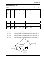
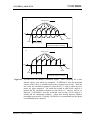
1
LS-DYNA KEYWORD USER’S MANUAL (Update) October 2004 Version 970 / Rev 5434 Copyright © 1992-2004 LIVERMORE SOFTWARE TECHNOLOGY CORPORATION All Rights Reserved Mailing Address: Livermore Software Technology Corporation 2876 Waverley Way Livermore, California 94551 Support Address: Livermore Software Technology Corporation 7374 Las Positas Road Livermore, California 94551 TEL: 925-449-2500 FAX: 925-449-2507 EMAIL: [email protected] Copyright © 1992-2004 by Livermore Software Technology Corporation All Rights Reserved *TABLE OF CONTENTS TABLE OF CONTENTS *AIRBAG....................................................................................................................................................1.1 *AIRBAG_WANG_NEFSKE.......................................................................................................1.2 *AIRBAG_HYBRID AND *AIRBAG_HYBRID_JETTING ......................................................1.10 *AIRBAG_ALE ..........................................................................................................................1.14 *CONSTRAINED ......................................................................................................................................2.1 *CONSTRAINED_BUTT_WELD................................................................................................2.2 *CONTROL................................................................................................................................................3.1 *CONTROL_ADAPTIVE.............................................................................................................3.2 *CONTROL_ALE.........................................................................................................................3.2 *CONTROL_BULK_VISCOSITY .............................................................................................3.11 *CONTROL_CONTACT............................................................................................................3.13 *CONTROL_DYNAMIC_RELAXATION ................................................................................3.19 *CONTROL_IMPLICIT_INERTIA_RELIEF ............................................................................3.21 *DEFINE.....................................................................................................................................................4.1 *DEFINE_SPOTWELD_FAILURE_RESULTANTS ..................................................................4.2 *DEFINE_SPOTWELD_RUPTURE_STRESS............................................................................4.4 *ELEMENT................................................................................................................................................5.1 *ELEMENT_BEAM_{OPTION}_{OPTION} .............................................................................5.2 *ELEMENT_SEATBELT_PRETENSIONER............................................................................5.12 *HOURGLASS...........................................................................................................................................6.1 *INITIAL ....................................................................................................................................................7.1 *INITIAL_STRESS_SECTION....................................................................................................7.2 *KEYWORD ..............................................................................................................................................8.1 *KEYWORD_OPTION {MEMORY} .........................................................................................8.1 *MAT ..........................................................................................................................................................9.1 *MAT_FABRIC ............................................................................................................................9.2 *MAT_BILKHU/DUBOIS_FOAM ..............................................................................................9.9 *MAT_PLASTICITY_WITH_DAMAGE_{OPTION} ..............................................................9.12 LS-DYNA Version 970 Update I.1 *TABLE OF CONTENTS *MAT_SOFT_TISSUE_{OPTION}............................................................................................9.20 *MAT_SPOTWELD_{OPTION} ...............................................................................................9.25 *MAT_ANISOTROPIC_VISCOPLASTIC.................................................................................9.35 *MAT_MODIFIED_PIECEWISE_LINEAR_PLASTICITY_{OPTION} .................................9.41 *MAT_PLASTICITY_COMPRESSION_TENSION .................................................................9.45 *MAT_MODIFIED_HONEYCOMB..........................................................................................9.49 *MAT_BARLAT_YLD2000.......................................................................................................9.58 *MAT_1DOF_GENERALIZED_SPRING .................................................................................9.64 *MAT_RATE_SENSITIVE_COMPOSITE_FABRIC................................................................9.66 *MAT_ARUP_ADHESIVE ........................................................................................................9.71 *MAT_RESULTANT_ANISOTROPIC .....................................................................................9.74 *MAT_SIMPLIFIED_RUBBER/FOAM.....................................................................................9.78 RESTART INPUT DATA........................................................................................................................10.1 *CHANGE_OPTION...................................................................................................................10.1 RIGID_BODY_INERTIA ...........................................................................................................10.2 I.2 LS-DYNA Version 970 Update *AIRBAG *AIRBAG Purpose: Define an airbag or control volume. The keyword *AIRBAG provides a way of defining thermodynamic behavior of the gas flow into the airbag as well as a reference configuration for the fully inflated bag. The keyword cards in this section are defined in alphabetical order: *AIRBAG_OPTION1_{OPTION2}_{OPTION3}_{OPTION4} *AIRBAG_OPTION1_{OPTION2}_{OPTION3}_{OPTION4} OPTION1 specifies one of the following thermodynamic relationships: There were three changed keyword cards in this section: WANG_NEFSKE HYBRID_JETTING HYBRID_CHEMKIN ALE LS-DYNA Version 970 Update 1.1 (AIRBAG) *AIRBAG *AIRBAG_WANG_NEFSKE Additional 4 cards are required for all WANG_NEFSKE models Card 1 1 2 3 4 5 6 7 8 CV CP T LCT LCMT TVOL LCDT IABT F F F I I F I F Default none none 0. 0 none 0. 0. not used Card 2 1 2 3 4 5 6 7 8 C23 LCC23 A23 LCA23 CP23 LCCP23 AP23 LCAP23 F I F I F I F I Default none 0 none 0 none 0 0.0 0 Card 3 1 2 3 4 5 6 7 8 PE RO GC LCEFR POVER PPOP OPT KNKDN F F F I F F F I none none none 0 0.0 0.0 0.0 0 Variable Type Variable Type Variable Type Default 1.2 (AIRBAG) LS-DYNA Version 970 Update *AIRBAG If the inflator is modeled, LCMT=0, define, the following card. If not, define but leave blank. Card 4 Variable Type Default 1 2 3 4 5 6 IOC IOA IVOL IRO IT LCBF F F F F F I none none none none none none 7 8 Define the following card if and only if CV=0. This option allows temperature dependent heat capacities to be defined. See below. Card 5 Variable Type Default 1 2 3 4 5 TEXT A B MW GASC F F F F F none none none none none 6 7 8 Define the following card if and only if the POP option is specified. Use this option to specify additional criteria for initiating exit flow from the airbag. Card 5 Variable Type Default 1 2 3 4 5 6 7 8 TDP AXP AYP AZP AMAGP TDURP TDA RBIDP F F F F F F F I 0.0 0.0 0.0 0.0 0.0 0.0 0.0 none LS-DYNA Version 970 Update 1.3 (AIRBAG) *AIRBAG VARIABLE DESCRIPTION CV Heat capacity at constant volume CP Heat capacity at constant pressure T Temperature of input gas. For temperature variations a load curve, LCT, may be defined. LCT Optional load curve number defining temperature of input gas versus time. This overides columns T. LCMT Load curve specifying input mass flow rate or tank pressure versus time. If the tank volume, TVOL, is nonzero the curve ID is assumed to be tank pressure versus time. If LCMT=0, then the inflator has to be modeled, see Card 4. During the dynamic relaxation phase the airbag is ignored unless the curve is flagged to act during dynamic relaxation. TVOL Tank volume which is required only for the tank pressure versus time curve, LCMT. LCDT Load curve for time rate of change of temperature (dT/dt) versus time. IABT Initial airbag temperature. (Optional, generally not defined.) C23 Vent orifice coefficient which applies to exit hole. Set to zero if LCC23 is defined below. LCC23 The absolute value, |LCC23|, is a load curve ID. If the ID is positive, the load curve defines the vent orifice coefficient which applies to exit hole as a function of time. If the ID is negative, the vent orifice coefficient is defined as a function of relative pressure, Pair / Pbag , see [Anagonye and Wang, 1999]. A nonzero value for C23 overrides LCC23. A23 If defined as a positive number, A23 is the vent orifice area which applies to exit hole. If defined as a negative number, the absolute value |A23| is a part ID, see [Anagonye and Wang, 1999]. The area of this part becomes the vent orifice area. Set A23 to zero if LCA23 is defined below. LCA23 Load curve number defining the vent orifice area which applies to exit hole as a function of absolute pressure. A nonzero value for A23 overrides LCA23. CP23 Orifice coefficient for leakage (fabric porosity). Set to zero if LCCP23 is defined below. LCCP23 Load curve number defining the orifice coefficient for leakage (fabric porosity) as a function of time. A nonzero value for CP23 overrides LCCP23. AP23 LCAP23 1.4 (AIRBAG) Area for leakage (fabric porosity) Load curve number defining the area for leakage (fabric porosity) as a function of (absolute) pressure. A nonzero value for AP23 overrides LCAP23. LS-DYNA Version 970 Update *AIRBAG VARIABLE DESCRIPTION PE Ambient pressure RO Ambient density GC Gravitational conversion constant (mandatory - no default). If consistent units are being used for all parameters in the airbag definition then unity should be input. LCEFR Optional curve for exit flow rate versus (gauge) pressure POVER Initial relative overpressure (gauge), Pover in control volume PPOP Pop Pressure: relative pressure (gauge) for initiating exit flow, Ppop OPT Fabric venting option, if nonzero CP23, LCCP23, AP23, and LCAP23 are set to zero. EQ. 1: Wang-Nefske formulas for venting through an orifice are used. Blockage is not considered. EQ. 2: Wang-Nefske formulas for venting through an orifice are used. Blockage of venting area due to contact is considered. EQ. 3: Leakage formulas of Graefe, Krummheuer, and Siejak [1990] are used. Blockage is not considered. EQ. 4: Leakage formulas of Graefe, Krummheuer, and Siejak [1990] are used. Blockage of venting area due to contact is considered. EQ. 5: Leakage formulas based on flow through a porous media are used. Blockage is not considered. EQ. 6: Leakage formulas based on flow through a porous media are used. Blockage of venting area due to contact is considered. EQ. 7: Leakage is based on gas volume outflow versus pressure load curve [Lian, 2000]. Blockage is not considered. EQ. 8: Leakage is based on gas volume outflow versus pressure load curve [Lian, 2000]. Blockage of venting area due to contact is considered. KNKDN Optional load curve ID defining the knock down pressure scale factor versus time. This option only applies to jetting. The scale factor defined by this load curve scales the pressure applied to airbag segments which do not have a clear line-of-sight to the jet. Typically, at very early times this scale factor will be less than unity and equal to unity at later times. The full pressure is always applied to segments which can see the jets. IOC Inflator orifice coefficient IOA Inflator orifice area LS-DYNA Version 970 Update 1.5 (AIRBAG) *AIRBAG VARIABLE DESCRIPTION IVOL Inflator volume IRO Inflator density IT Inflator temperature LCBF Load curve defining burn fraction versus time TEXT Ambient temperature. A First heat capacity coefficient of inflator gas (e.g., Joules/mole/oK) B Second heat capacity coefficient of inflator gas, (e.g., Joules/mole/oK2) MW GASC Molecular weight of inflator gas (e.g., Kg/mole). Universal gas constant of inflator gas (e.g., 8.314 Joules/mole/oK) TDP Time delay before initiating exit flow after pop pressure is reached. AXP Pop acceleration magnitude in local x-direction. EQ. 0.0: Inactive. AYP Pop acceleration magnitude in local y-direction. EQ. 0.0: Inactive. AZP Pop acceleration magnitude in local z-direction. EQ. 0.0: Inactive. AMAGP Pop acceleration magnitude. EQ. 0.0: Inactive. TDURP Time duration pop acceleration must be exceeded to initiate exit flow. This is a cumulative time from the beginning of the calculation, i.e., it is not continuous. TDA Time delay before initiating exit flow after pop acceleration is exceeded for the prescribed time duration. RBIDP Part ID of the rigid body for checking accelerations against pop accelerations. 1.6 (AIRBAG) LS-DYNA Version 970 Update *AIRBAG Remarks: The gamma law equation of state for the adiabatic expansion of an ideal gas is used to determine the pressure after preload: p = (γ − 1)ρ e where p is the pressure, ρ is the density, e is the specific internal energy of the gas, and γ is the ratio of the specific heats: γ = cp cv where cv is the specific heat at constant volume, and cp is the specific heat at constant pressure. A pressure relation is defined: Q= pe p where pe is the external pressure and p is the internal pressure in the bag. A critical pressure relationship is defined as: Qcrit 2 = γ +1 γ γ −1 where γ is the ratio of specific heats: γ = cp cv If Q ≤ Qcrit then Q = Qcrit Wang and Nefske define the mass flow through the vents and leakage by ( ) ( ) m& 23 = C23 A23 γ −1 1 γR p Q γ 2 gc 1−Q γ R T2 γ −1 ′ = C23 ′ A23 ′ m& 23 γ −1 1 γR p Q γ 2 gc 1− Q γ R T2 γ −1 and LS-DYNA Version 970 Update 1.7 (AIRBAG) *AIRBAG It must be noted that the gravitational conversion constant has to be given in consistent units. As an alternative to computing the mass flow out of the bag by the Wang-Nefske model, a curve for the exit flow rate depending on the internal pressure can be taken. Then, no definitions for C23, LCC23, A23, LCA23, CP23, LCCP23, AP23, and LCAP23 are necessary. The airbag inflator assumes that the control volume of the inflator is constant and that the amount of propellant reacted can be defined by the user as a tabulated curve of fraction reacted versus time. A pressure relation is defined: γ Qcrit p 2 γ −1 = c = pi γ + 1 where pc is a critical pressure at which sonic flow occurs, pI , is the inflator pressure. The exhaust pressure is given by pe = pa if pe = pc if pa ≥ pc pa < pc where pa is the pressure in the control volume. The mass flow into the control volume is governed by the equation: m& in = CO AO 2 p I ρ I γ +1 γ2 g cγ Q − Q γ γ −1 where CO , AO , and ρI are the inflator orifice coefficient, area, and gas density, respectively. If OPT is defined, then for OPT set to 1 or 2 the mass flow rate out of the bag, m& out is given by: m& out = gc ⋅ nairmats ∑ n =1 ( FLC (t )n ⋅ FAC ( p)n ⋅ Arean ) ⋅ 2 pρ ( 2 k γ Q −Q γ −1 γ +1 γ ) where, ρ is the density of airbag gas, nairmats is the number of fabrics used in the airbag, and Arean is the current unblocked area of fabric number n. If OPT set to 3 or 4 then: nairmats m& out = ∑ ( FLC (t ) n ⋅ FAC ( p ) n ⋅ Arean ) ⋅ 2 ( p − pext ) ρ n =1 and for OPT set to 5 or 6: 1.8 (AIRBAG) LS-DYNA Version 970 Update *AIRBAG nairmats m& out = ∑ ( FLC (t )n ⋅ FAC ( p ) n ⋅ Arean ) ⋅ ( p − pext ) n =1 and of OPT set to 7 or 8 then: m& out = nairmats ∑ FLC (t ) n ⋅ FAC ( p ) n ⋅ Arean ⋅ ρ n n =1 where FAC ( p ) n is the gas volume outflow through a unit area per unit time. Multiple airbags may share the same part ID since the area summation is over the airbag segments whose corresponding part ID’s are known. Currently, we assume that no more than ten materials are used per bag for purposes of the output. This constraint can be eliminated if necessary. The total mass flow out will include the portion due to venting, i.e., constants C23 and A23 or their load curves above. If CV=0. then the constant-pressure specific heat is given by: cp = (a + bT ) MW and the constant-volume specific heat is then found from: cv = c p − LS-DYNA Version 970 Update R MW 1.9 (AIRBAG) *AIRBAG *AIRBAG_HYBRID and *AIRBAG_HYBRID_JETTING Additional cards required for HYBRID and HYBRID_JETTING options Variable 1 2 3 4 5 ATMOST ATMOSP ATMOSD GC CC F F F F F none none none none 1.0 1 2 3 4 C23 LCC23 A23 F I none Type Default Variable Type Default Variable Type Default 1.10 (AIRBAG) 6 7 8 5 6 7 8 LCA23 CP23 LCP23 AP23 LCAP23 F I F I F I 0 none 0 none 0 none 0 1 2 3 4 5 6 7 8 OPT PVENT NGAS I F I none none none LS-DYNA Version 970 Update *AIRBAG Define 2*NGAS cards below, two for each gas type. Variable 1 2 LCIDM LCIDT I I none 1 Type Default Variable 3 4 5 6 7 8 MW INITM A B C F F F F F F none not used none none none none none 2 3 4 5 6 7 8 FMASS Type F Default none VARIABLE DESCRIPTION ATMOST Atmospheric temperature ATMOSP Atmospheric pressure ATMOSD Atmospheric density GC Universal molar gas constant CC Conversion constant EQ: .0 Set to 1.0. C23 Vent orifice coefficient which applies to exit hole. Set to zero if LCC23 is defined below. LCC23 The absolute value, |LCC23|, is a load curve ID. If the ID is positive, the load curve defines the vent orifice coefficient which applies to exit hole as a function of time. If the ID is negative, the vent orifice coefficient is defined as a function of relative pressure, Pair / Pbag , see [Anagonye and Wang, 1999]. A nonzero value for C23 overrides LCC23. LS-DYNA Version 970 Update 1.11 (AIRBAG) *AIRBAG VARIABLE DESCRIPTION A23 If defined as a positive number, A23 is the vent orifice area which applies to exit hole. If defined as a negative number, the absolute value |A23| is a part ID, see [Anagonye and Wang, 1999]. The area of this part becomes the vent orifice area. Set A23 to zero if LCA23 is defined below. LCA23 Load curve number defining the vent orifice area which applies to exit hole as a function of absolute pressure. A nonzero value for A23 overrides LCA23. CP23 Orifice coefficient for leakage (fabric porosity). Set to zero if LCCP23 is defined below. LCCP23 Load curve number defining the orifice coefficient for leakage (fabric porosity) as a function of time. A nonzero value for CP23 overrides LCCP23. AP23 Area for leakage (fabric porosity) LCAP23 Load curve number defining the area for leakage (fabric porosity) as a function of (absolute) pressure. A nonzero value for AP23 overrides LCAP23. OPT Fabric venting option, if nonzero CP23, LCCP23, AP23, and LCAP23 are set to zero. EQ. 1: Wang-Nefske formulas for venting through an orifice are used. Blockage is not considered. EQ. 2: Wang-Nefske formulas for venting through an orifice are used. Blockage of venting area due to contact is considered. EQ. 3: Leakage formulas of Graefe, Krummheuer, and Siejak [1990] are used. Blockage is not considered. EQ. 4: Leakage formulas of Graefe, Krummheuer, and Siejak [1990] are used. Blockage of venting area due to contact is considered. EQ. 5: Leakage formulas based on flow through a porous media are used. Blockage is not considered. EQ. 6: Leakage formulas based on flow through a porous media are used. Blockage of venting area due to contact is considered. PVENT Gauge pressure when venting begins NGAS Number of gas inputs to be defined below. (Including initial air) LCIDM Load curve ID for inflator mass flow rate (eq. 0 for gas in the bag at time 0) GT.0: piece wise linear interpolation LT.0: cubic spline interpolation LCIDT Load curve ID for inflator gas temperature (eq.0 for gas in the bag at time 0) GT.0: piece wise linear interpolation LT.0: cubic spline interpolation 1.12 (AIRBAG) LS-DYNA Version 970 Update *AIRBAG VARIABLE BLANK MW INITM DESCRIPTION (not used) Molecular weight Initial mass fraction of gas component A Coefficient for molar heat capacity of inflator gas at constant pressure, (e.g., Joules/mole/oK) B Coefficient for molar heat capacity of inflator gas at constant pressure, (e.g., Joules/mole/oK2) C Coefficient for molar heat capacity of inflator gas at constant pressure, (e.g., Joules/mole/oK3) FMASS Fraction of additional aspirated mass. LS-DYNA Version 970 Update 1.13 (AIRBAG) *AIRBAG *AIRBAG_ALE Purpose: The input in this section provides a simplified approach to defining the deployment of the airbag using the ALE capabilities with an option to switch from the initial ALE method to control volume (CV) method (*AIRBAG_HYBRID) at a chosen time. An enclosed airbag (and possibly the airbag canister/compartment and/or a simple representation of the inflator) shell structure interacts with the inflator gas(es). This definition provides a single fluid to structure coupling for the airbag-gas interaction during deployment in which the CV input data may be used directly. Card Format Card 1 7 8 SIDTYP MWD SPSF I I F F Default none none 0 0 Remarks 1 Variable Type 1 2 SID 3 VARIABLE SID SIDTYP MWD SPSF 1.14 (AIRBAG) 4 5 6 DESCRIPTION Set ID as defined on *AIRBAG card. This set ID contains the Lagrangian elements (segments) which make up the airbag and possibly the airbag canister/compartment and/or a simple representation of the inflator. See remark 1. Set type: EQ.0: Segment set. EQ.1: Part set. Mass weighted damping factor, D. This is used during the CV phase for *AIRBAG_HYBRID. Stagnation pressure scale factor, 0 ≤ γ ≤ 1 . This is used during the CV phase for *AIRBAG_HYBRID. LS-DYNA Version 970 Update *AIRBAG Parameters for defining ambient environment. Card 2 Variable ATMOST ATMOSP GC CC TNKVOL TNKFINP Type F F F F F F Default 0. 0. none 1.0 0.0 0.0 Remarks 2 2 10 10 VARIABLE DESCRIPTION ATMOST Atmospheric ambient temperature. See remark 2. ATMOSP Atmospheric ambient pressure. See remark 2. GC Universal molar gas constant. CC Conversion constant. If EQ: .0 Set to 1.0. TNKVOL Tank volume from the inflator tank test – or – Inflator canister volume. See remark 10. Option 1: (LCVEL = 0) This is defined as Tank volume (must also define TNKFINP). Inlet gas velocity is estimated by LSDYNA method (testing). Option 2: (LCVEL = 0) This is defined as estimated inflator canister volume (must NOT define TNKFINP). Inlet gas velocity is estimated automatically by the Lian-Bhalsod-Olovsson method. Option 3: (LCVEL .NE. 0) This must be left blank. TNKFINP Tank final pressure from the inflator tank test data. Only define this parameter for option 1 of TNKVOL definition above. See remark 10. LS-DYNA Version 970 Update 1.15 (AIRBAG) *AIRBAG Parameters for coupling, see keyword *CONSTRAINED_LAGRANGE_IN_SOLID. Card 3 1 2 3 NQUAD CTYPE PFAC Type I I F F F I I F Default 4 4 0.1 0.0 0.3 0 2 0.1 Remarks 13 13 14 Variable VARIABLE 4 FRIC 5 FRCMIN 6 7 NORMTYP ILEAK 8 PLEAK DESCRIPTION NQUAD Number of (quadrature) coupling points for coupling Lagrangian slave parts to ALE master solid parts. If NQUAD=n, then nXn coupling points will be parametrically distributed over the surface of each Lagrangian slave segment (default=4). See remark 13. CTYPE Coupling type (default=4, see remark 13): EQ.4: (default) penalty coupling with DIREC=2 implied. EQ.6: penalty coupling in which DIREC is automatically set to DIREC=1 for the unfolded region and DIREC=2 for folded region. PFAC Penalty factor. PFAC is a scale factor for scaling the estimated stiffness of the interacting (coupling) system. It is used to compute the coupling forces to be distributed on the slave and master parts. If positive real: Fraction of estimated critical stiffness default=0.1). If negative integer, -n: Refers to load curve ID n. The curve defines the relative coupling pressure (y-axis) as a function of the tolerable fluid penetration distance (x-axis). FRIC Coupling coefficient of friction. FRCMIN Minimum fluid volume fraction in an ALE element to activate coupling (default is 0.3). NORMTYP Penalty coupling spring direction (DIREC 1 and 2): EQ.0: normal vectors are interpolated from nodal normals (default) EQ.1: normal vectors are interpolated from segment normals. 1.16 (AIRBAG) LS-DYNA Version 970 Update *AIRBAG VARIABLE DESCRIPTION ILEAK Leakage control flag. Default=2 (with energy compensation). PLEAK Leakage control penalty factor (default=0.1) Parameters for airbag venting hole Card 4 1 2 3 4 IVSETID IVTYPE IBLOCK VNTCOF Type I I I F Default 0 0 0 0.0 Remarks 4 5 6 Variable VARIABLE 5 6 7 8 DESCRIPTION IVSETID Set ID defining the venting hole surface(s). See remark 4. IVTYPE Set type of IVSETID: EQ.0: Part Set (default). EQ:1: Part ID. EQ:2: Segment Set. IBLOCK Flag for considering blockage effects for porosity and vents (remark 5): EQ:0: no (blockage is NOT considered, default). EQ:1: yes (blockage is considered). VNTCOF Vent Coefficient for scaling the flow. See remark 6. LS-DYNA Version 970 Update 1.17 (AIRBAG) *AIRBAG Parameters for ALE mesh automatic definition and its transformation. Card 5 Variable NX/IDA NY/IDG NZ MOVERN ZOOM I I I I I Default None None None 0 0 Remarks 7 7 7 8 9 Type VARIABLE DESCRIPTION NX/IDAIR Option 1: NX is defined (as the number of ALE elements to be. generated in the x direction). This must goes together with option 1 for NY and NZ. Option 2: IDAIR is defined as Part ID of the initial air mesh. See remark 7. NY/IDGAS Option 1: NY is defined (as the number of ALE elements to be. generated in the y direction). This must goes together with option 1 for NX and NZ. Option 2: IDGAS is defined as Part ID of the initial gas mesh. See remark 7. NZ Option 1: NZ is defined (as the number of ALE elements to be. generated in the z direction). This must goes together with option 1 for NX and NY. Option 2: Leave blank. See remark 7. MOVERN ZOOM 1.18 (AIRBAG) ALE mesh automatic motion option (remark 8): EQ.0: ALE mesh is fixed in space. GT.0: Node group id. See *ALE_REFERENCE_SYSTEM_NODE ALE mesh can be moved with PRTYP=5, mesh motion follows a coordinate system defined by 3 reference nodes. ALE mesh automatic expansion option (remark 9): EQ.0: do not expand ALE mesh EQ.1: Expand/contract ALE mesh by keeping all airbag parts contained within the ALE mesh (equivalent to PRTYP=9). LS-DYNA Version 970 Update *AIRBAG Define card 5a and 5b if NZ > 0 Card 5a 1 2 3 4 5 6 Variable X0 Y0 Z0 X1 Y1 Z1 F F F F F F Default None None None None None None Card 5b 1 2 3 4 5 6 Variable X2 Y2 Z2 Z3 Y3 Z3 F F F F F F None None None None None None Type Type Default VARIABLE 7 8 7 8 DESCRIPTION X0, Y0, Z0 Coordinates of origin for ALE mesh generation (node0). X1, Y1, Z1 Coordinates of point 1 for ALE mesh generation (node1). node0=>node1 = x X2, Y2, Z2 Coordinates of point 2 for ALE mesh generation (node2). node0=>node2 = y X3, Y3, Z3 Coordinates of point 3 for ALE mesh generation(node3). node0=>node3 = z x1,y1,z1 x3,y3,z31 N x2,y2,z21 Ny LS-DYNA Version 970 Update N x0,y0,z0 1.19 (AIRBAG) *AIRBAG Card 6 Variable SWTIME HG Type F F I I I I I Default 0. 0. 0 0 0 0 0 Remarks 3 10 11 VARIABLE SWTIME HG NAIR NGAS NORIF LCVEL LCT DESCRIPTION Time to switch from ALE method to control volume (CV) method. Once switched, a method similar to that used by the *AIRBAG_HYBRID card is used. EQ.0.0: switch to CV method at time=0.0. EQ.blank: switch time is set at 1.0E16 (ALE method is used). EQ.t: switch from ALE to CV method at time=t. Hourglass control for ALE fluid mesh(es). NAIR Number of Air components. For example, this equals 2 in case air contains 80% of N2 and 20% of O2. If air is defined as 1 single gas then NAIR=1. NGAS Number of inflator Gas components. NORIF Number of point sources or orifices (defined below) EQ.n: will require n lines of card 9 definitions below, one for each point source.. LCVEL Load curve ID for inlet velocity (see also TNKVOL & TNKFINP of card 2 above). This is the same estimated velocity curve used in *SECTION_POINT_SOURCE_MIXTURE card. LCT 1.20 (AIRBAG) Load curve ID for inlet gas temperature (see *AIRBAG_HYBRID). LS-DYNA Version 970 Update *AIRBAG Define NAIR cards below for air component Card 7 1 2 Variable 3 4 MWAIR 5 INITM 6 7 8 AIRA AIRB AIRC Type F F F F F Default 0 0 0 0. 0. 12 12 12 Remarks VARIABLE MWAIR DESCRIPTION Molecular weight of air component INITA Initial Mass Fraction of Air component(s) AIRA First Coefficient of molar heat capacity at constant pressure (e.g., J/mole/K, remark 12). AIRB Second Coefficient of molar heat capacity at constant pressure (e.g., J/mole/K2, remark 12). AIRC Third Coefficient of molar heat capacity at constant pressure (e.g., J/mole/K3, remark 12). LS-DYNA Version 970 Update 1.21 (AIRBAG) *AIRBAG Define NGAS cards below for the GAS components Cards 8… Variable 1 LCMF Type 2 3 4 5 MWGAS 6 7 GASA GASB 8 GASC I F F F F Default none 0 0 0. 0. Remarks 11 12 12 12 VARIABLE LCMF MWGAS DESCRIPTION Load curve ID for mass flow rate (see *AIRBAG_HYBRID, e.g., kg/s). Molecular weight of inflator gas components. GASA First Coefficient of molar heat capacity at constant pressure (e.g., J/mole/K, remark 12). GASB Second Coefficient of molar heat capacity at constant pressure (e.g., J/mole/K2, remark 12). GASC Third Coefficient of molar heat capacity at constant pressure (e.g., J/mole/K3, remark 12). 1.22 (AIRBAG) LS-DYNA Version 970 Update *AIRBAG Define NORIF cards below for each point source Cards 9… Variable 1 NODEID 2 3 VECID ORIFARE Type I I I Default 0 0 0 VARIABLE NODEID VECID ORIFARE 4 5 6 7 8 DESCRIPTION The node ID defining the point source. The vector ID defining the direction of flow at the point source. The orifice area at the point source. Remarks: 1. 2. 3. 4. 5. 6. 7. This set ID typically contains the Lagrangian segments of the 3 parts that are coupled to the inflator gas: airbag, airbag canister (compartment), inflator. As in all control-volume, orientation of elements representing bag and canister should point outward. During the ALE phase the segment normal will be reversed automatically for fluid-structure coupling. However, the orientation of inflator element normal vectors should point to its center, Fig. 2. Atmospheric density for the ambient gas (air) can be computed from ρ amb = Pamb ( R * Tamb ) Since ALL ALE related activities will be turned off after the switch from ALE method to control-volume method, no other ALE coupling will exist beyond t=SWTIME. Vent definition will be used for ALE venting. Upon switching area of the segments will be used for venting as a23 in *AIRBAG_HYBRID. Fabric porosity for ALE and *AIRBAG_HYBRID can be defined on MAT_FABRIC. Define FLC and FAC on *MAT_FABRIC. FVOPT 7 and 8 will be used for both ALE and *AIRBAG_HYBRID. IBLOCK=0 will use FVOPT=7 and IBLOCK=1 will use FVOPT=8. VCOF will be used to scale the vent area for ALE venting and this coefficient will be used as vent coefficient c23 for *AIRBAG_HYBRID upon switching. If Nz, Ny and Nz are defined (option 1), card 5a and card 5b should be defined to let LSDYNA generate the mesh for ALE. Alternatively if Nz is 0 (option 2), then Nx=IDAIR and Ny=IDGAS. In the later case the user need to supply the ALE mesh whose PID=IDAIR. LS-DYNA Version 970 Update 1.23 (AIRBAG) *AIRBAG 8. 9. 10. 11. 12. 13. 14. If the airbag moves with the vehicle, set MOVERN=GROUPID, this GROUPID is defined using *ALE_REFERENCE_SYSTEM_NODE. The 3 nodes defined in ALE_REFERENCE_SYSTEM_NODE will be used to transform the ALE mesh. The point sources will also follow this motion. This simulates PRTYP=5 in the *ALE_REFERENCE_SYSTEM_GROUP card. Automatic expansion/contraction of the ALE mesh to follow the airbag expansion can be turned on by setting zoom=1. This feature is particularly useful for fully folded airbags requiring very fine ale mesh initially. As the airbag inflates the ale mesh will be automatically scaled such that the airbag will be contained within the ALE mesh. This simulates PRTYP=9 in the *ALE_REFERENCE_SYSTEM_GROUP card. There are 3 methods for defining the inlet gas velocity: Option 1: define LCVEL = 0 Î TNKVOL = Tank volume, and TNKFINP = Tank final pressure from tank test data. Inlet gas velocity is estimated by LSDYNA method (testing). Option 2: define LCVEL = 0 Î TNKVOL = inflator can volume, and TNKFINP = blank. Inlet gas velocity is estimated automatically by Lian-Bhalsod-Olovsson method. Option 3: define LCVEL = n Î TNKVOL =0, and TNKFINP = 0. Inlet gas velocity is defined by user via a load curve ID = n. LCT and LCIDM should have the same number of sampling points. The molar heat capacity as a function of temperature is computed from CP = A + BT 2 + CT 3 / MW A = CP 0 Sometimes CTYPE=6 may be used for complex folded airbag. NQUAD=2 may be used as a starting value and increase as necessary depending on the relative mesh resolutions of the Lagrangrian and ALE meshes. Use a load curve for PFAC whenever possible. It tends to be more robust. Shell normals should point outwards Bag fabric Inflator Canister Figure XXXX 1.24 (AIRBAG) LS-DYNA Version 970 Update *AIRBAG EXAMPLE 1: $...|....1....|....2....|....3....|....4....|....5....|....6....|....7....|....8 *AIRBAG_ALE $#1 SID SIDTYPE NONE NONE NONE NONE MWD SPSF 123 1 0 0 0 0 0.0 0.0 $#2 ATMOST ATMOSP NONE GC CC TNKVOL TNKFP 298.15 1.0132E-4 0 8.314 0.0 0.0 0.0 $#3 NQUAD CTYPE PFAC FRIC FRCMIN NORMTYPE ILEAK PLEAK 4 4 -1000 0.0 0.3 0 2 0.1 $#4 VSETID IVSETTYP IBLOCK VENTCOEF 1 2 0 1.00 $#5NXIDAIR NYIDGAS NZ MOVERN ZOOM 50000 50003 0 0 0 $#6 SWTIME NONE HG NAIR NGAS NORIF LCVEL LCT 1000.00 0.000 1.e-4 1 1 8 2002 2001 $#7 AIR NONE NONE MWAIR INITM AIRA AIRB AIRC 0 0 0 0.02897 1.00 29.100 0.00000 0.00000 $#8 GASLCM NONE NONE MWGAS NONE GASA GASB GASC 2003 0 0 0.0235 0 28.000 0.00000 0.00000 $#9 NODEID VECTID ORIFAREA 100019 1 13.500000 100020 2 13.500000 100021 3 13.500000 100022 4 13.500000 100023 5 13.500000 100024 6 13.500000 100017 7 13.500000 100018 8 13.500000 $ PFAC CURVE = penalty factor curve. *DEFINE_CURVE $ lcid sidr sfa sfo offa offo dattyp 1000 0 0.0 2.0 0.0 0.0 $ a1 o1 0.0 0.00000000 1.0000000 4.013000e-04 *SET_SEGMENT_TITLE vent segments (defined in IVSETID) 1 0.0 0.0 0.0 0.0 1735 1736 661 1697 0.0 0.0 0.0 0.0 1735 2337 1993 1736 0.0 0.0 0.0 0.0 1735 1969 1988 2337 0.0 0.0 0.0 0.0 1735 1697 656 1969 0.0 0.0 0.0 0.0 *DEFINE_VECTOR $# vid xt yt zt xh yh zh 1 0.0 0.0-16.250000 21.213200 21.213200-16.250000 2 0.0 0.0-16.250000 30.000000-1.000e-06-16.250000 3 0.0 0.0-16.250000 21.213200-21.213200-16.250000 4 0.0 0.0-16.250000-1.000e-06-30.000000-16.250000 5 0.0 0.0-16.250000-21.213200-21.213200-16.250000 6 0.0 0.0-16.250000-30.0000001.0000e-06-16.250000 7 0.0 0.0-16.250000-21.213200 21.213200-16.250000 8 0.0 0.0-16.2500001.0000e-06 30.000000-16.250000 $...|....1....|....2....|....3....|....4....|....5....|....6....|....7....|....8 In this example, pre-existing background air mesh with part ID 50000 and gas mesh with part ID 50003 are used. Thus NZ = 0. There is no mesh motion nor expansion allowed. A inlet gas velocity curve is provided. LS-DYNA Version 970 Update 1.25 (AIRBAG) *AIRBAG EXAMPLE 2: $...|....1....|....2....|....3....|....4....|....5....|....6....|....7....|....8 $ SIDTYP: 0=SGSID; 1=PSID *AIRBAG_ALE $#1 SID SIDTYPE NONE NONE NONE NONE MWD SPSF 1 1 0 0. 0. 0. 0. 0. $#2 ATMOST ATMOSP NONE GC CC TNKVOL TNKFP 298. 101325. 0.0 8.314 1. 6.0E-5 0 $#3 NQUAD CTYPE PFAC FRIC FRCMIN NORMTYPE ILEAK PLEAK 2 6 -321 0.0 0.3 1 2 0.1 $#4 VSETID IVSETTYP IBLOCK VENTCOEF 0 0 0 0 $#5NXIDAIR NYIDGAS NZ MOVERN ZOOM 11 11 9 $5b x0 y0 z0 x1 y1 z1 NOT-USED NOT-USED -0.3 -0.3 -0.135 0.3 -0.3 -0.135 $5c x2 y2 z2 x3 y3 z3 NOT-USED NOT-USED -0.3 0.3 -0.135 -0.3 -0.3 0.39 $#6 SWTIME NONE HG NAIR NGAS NORIF LCVEL LCT 0.04000 0.005 1.e-4 2 1 1 0 2 $#7 AIR NONE NONE MWAIR INITM AIRA AIRB AIRC 0.028 0.80 27.296 0.00523 0.032 0.20 25.723 0.01298 $#8 GASLCM NONE NONE MWGAS NONE GASA GASB GASC 1 0.0249 29.680 0.00880 $#9 NODEID VECTID ORIFAREA 9272 1 1.00e-4 $ Lagrangian shell structure to be coupled to the inflator gas *SET_PART_LIST 1 0.0 0.0 0.0 0.0 1 2 3 *DEFINE_VECTOR $0.100000E+01, 10.000000000 $ vid xt yt zt xh yh zh 1 0.0 0.0 0.0 0.0 0.0 0.100000 $ bag penetration ~ 1 mm <====> P_coup ~ 500000 pascal ==> ~ 5 atm *DEFINE_CURVE $ lcid sidr sfa sfo offa offo dattyp 321 0 0.0 0.0 0.0 0.0 $ a1 o1 0.0 0.0 0.00100000 5.0000000e+05 $...|....1....|....2....|....3....|....4....|....5....|....6....|....7....|....8 In this example, LS-DYNA automatically creates the background ALE mesh with: NX = 11 elements in the x direction. NY = 11 elements in the y direction. NZ = 9 elements in the z direction. This ALE mesh is generated based on the 4 given reference nodes defined in cards 5b and 5c. Note that LCVEL=0 and TNKVOL=6.0E-5 (inflator volume is small relative to the airbag volume, may be estimated at ~ 1/200 of the airbag volume as a first approximation). Since TNKFINP = 0 Î the velocity is computed based on the Lian-Bhalsod-Olovsson method automatically. 1.26 (AIRBAG) LS-DYNA Version 970 Update *CONSTRAINED *CONSTRAINED The keyword *CONSTRAINED provides a way of constraining degrees of freedom to move together in some way. There is one changed keyword card in this section: *CONSTRAINED_BUTT_WELD LS-DYNA Version 970 Update 2.1 (CONSTRAINED) *CONSTRAINED *CONSTRAINED_BUTT_WELD *CONSTRAINED_BUTT_WELD Purpose: Define a line of coincident nodes that represent a structural butt weld between two parts defined by shell elements. Failure is based on nodal plastic strain for ductile failure and stress resultants for brittle failure. This input is much simpler than the alternative approach for defining butt welds, see *CONSTRAINED_GENERALIZED_WELD_BUTT. The local coordinate system, the effective length, and thickness for each pair of butt welded nodes are determined automatically in the definition below. In the GENERALIZED option these quantities must be defined in the input. Card Format Variable Type Default 1 2 3 4 5 SNSID MNSID EPPF SIGF BETA I I F F F none none 0. 1.e+16 1.0 1, 2 3, 4 3 3 Remarks VARIABLE 6 7 8 DESCRIPTION SNSID Slave node set ID, see *SET_NODE_OPTION. MNSID Master node set ID, see *SET_NODE_OPTION. EPPF Plastic strain at failure SIGF σf, stress at failure for brittle failure. BETA β, failure parameter for brittle failure. Remarks: 1. Nodes in the master and slave sets must be given in the order they appear as one moves along the edge of the surface. An equal number of coincident nodes must be defined in each set. In a line weld the first and last node in a string of nodes can be repeated in the two sets. If the first and last pair of nodal points are identical, a circular or closed loop butt weld is assumed. See Figure 6.1, where the line butt weld and closed loop weld are illustrated. 2.2 (CONSTRAINED) LS-DYNA Version 970 Update *CONSTRAINED *CONSTRAINED_BUTT_WELD 2. Butt welds may not cross. For complicated welds, this option can be combined with the input in *CONSTRAINED_GENERALIZED_WELD_BUTT to handle the case where crossing occurs. Nodes in a butt weld must not be members of rigid bodies. 3. If the average volume-weighted effective plastic strain in the shell elements adjacent to a node exceeds the specified plastic strain at failure, the node is released. Brittle failure of the butt welds occurs when: ( β σ2n + 3 τ 2n + τ2t ) ≥σf where σn τn τt σf β = = = = = normal stress (local x) shear stress in direction of weld (local y) shear stress normal to weld (local z) failure stress failure parameter Component σn is nonzero for tensile values only. The nodes defining the slave and master sides of the butt weld must coincide. The local z-axis at a master node is normal to the master side plane of the butt weld at the node, and the local y-axis is taken as the vector in the direction of a line connecting the mid-points of the line segments lying on either side of the master node. The normal vector is found by summing the unit normal vectors of all shell elements on the master side sharing the butt welded node. The direction of the normal vector at the node is chosen so that the x-local vector points towards the elements on the slave side in order to identify tensile versus compressive stresses. The thickness of the butt weld and length of the butt weld are needed to compute the stress values. The thickness is based on the average thickness of the shell elements that share the butt welded nodal pair, and the chosen length of the butt weld is shown in Figure 6.1. 4. Butt welds may be used to simulate the effect of failure along a predetermined line, such as a seam or structural joint. When the failure criterion is reached at a nodal pair, the nodes begin to separate. As this effect propagates, the weld will appear to “unzip,” thus simulating failure of the connection. LS-DYNA Version 970 Update 2.3 (CONSTRAINED) *CONSTRAINED local y-axis Repeated nodal point may start or end a butt weld line. This beginning or ending nodal point must exist in both and slave and master definitions. *CONSTRAINED_BUTT_WELD Length of butt weld Two coincident butt welded nodal points. Repeated nodal point pair must start and end circular butt weld. Any nodal pair in the circle can be used. Figure 6.1. Definition of butt welds are shown above. The butt weld can be represented by a line of nodal points or by a closed loop. 2.4 (CONSTRAINED) LS-DYNA Version 970 Update *CONTROL *CONTROL The keyword control cards are optional and can be used to change defaults, activate solution options such as mass scaling, adaptive remeshing, and an implicit solution; however, it is advisable to define the *CONTROL_TERMINATION card. The ordering of the control cards in the input file is arbitrary. To avoid ambiguities, define no more than one control card of each type. The keywords that have new options in this release are: *CONTROL_ADAPTIVE *CONTROL_BULK_VISCOSITY *CONTROL_CONTACT *CONTROL_DYNAMIC_RELAXATION *CONTROL_IMPLICIT_INERTIA_RELIEF LS-DYNA Version 970 Update 3.1 (CONTROL) *CONTROL *CONTROL_ADAPTIVE *CONTROL_ADAPTIVE Purpose: Activate adaptive meshing. The parts which are adaptively meshed are defined by *PART. See remarks below. Card Format Card 1 Variable 1 2 3 4 5 6 7 8 ADPFREQ ADPTOL ADPOPT MAXLVL TBIRTH TDEATH LCADP IOFLAG F F I I F F I I 1 3 0.0 0 0 Type Default none Card 2 10 20 10 20 1 2 3 4 5 6 7 8 ADPSIZE ADPASS IREFLG ADPENE ADPTH MEMORY ORIENT MAXEL F I I F F I I I 0 0 0.0 inactive inactive 0 inactive 3 4 5 6 7 8 IADPE90 NCFREQ IADPCL ADPCTL CBIRTH CDEATH Type I I I F F F Default 0 none 1 none 0.0 Variable Type Default Card Format (This card is optional). Card 3 Variable 1 3.2 (CONTROL) 2 10 20 LS-DYNA Version 970 Update *CONTROL *CONTROL_ADAPTIVE VARIABLE ADPFREQ DESCRIPTION Time interval between adaptive refinements, see Figure 8.1. ADPTOL Adaptive error tolerance in degrees for ADPOPT set to 1 or 2 below. If ADPOPT is set to 8, ADPTOL is the characteristic element size. ADPOPT Adaptive options: EQ.1: angle change in degrees per adaptive refinement relative to the surrounding elements for each element to be refined. EQ.2: total angle change in degrees relative to the surrounding element for each element to be refined. For example, if the adptol=5 degrees, the element will be refined to the second level when the total angle change reaches 5 degrees. When the angle change is 10 degrees the element will be refined to the third level. EQ.7: 3D r-adaptive remeshing for solid elements. Solid element type 13, a tetrahedron, is used in the adaptive remeshing process. A completely new mesh is generated which is initialized from the old mesh using a least squares approximation. The mesh size is currently based on the minimum and maximum edge lengths defined on the *CONTROL_REMESHING keyword input. This option remains under development, and, we are not sure of its reliability on complex geometries. EQ.8: 2D r-adaptive remeshing for axisymmetric and plane strain solid elements. A completely new mesh is generated which is initialized from the old mesh using a least squares approximation. The mesh size is currently based on the value, ADPTOL, which gives the characteristic element size. This option is based on earlier work by Dick and Harris [1992]. MAXLVL Maximum number of refinement levels. Values of 1, 2, 3, 4,... allow a maximum of 1, 4, 16, 64, ... elements, respectively, to be created for each original element. The refinement level can be overridden by *DEFINE_BOX_ADAPTIVE, or *DEFINE_SET_ADAPTIVE. TBIRTH Birth time at which the adaptive remeshing begins, see Figure 8.1. TDEATH Death time at which the adaptive remeshing ends, see Figure 8.1. LCADP Adaptive interval is changed as a function of time given by load curve ID, LCADP. If this option is nonzero, the ADPFREQ will be replaced by LCADP. The x-axis is time and the y-axis is the varied adaptive time interval. LS-DYNA Version 970 Update 3.3 (CONTROL) *CONTROL *CONTROL_ADAPTIVE VARIABLE DESCRIPTION IOFLAG Flag to generate adaptive mesh at exit including *NODE, *ELEMENT, *SHELL, and *BOUNDARY_, *CONTACT_NODE_, and *CONSTRAINED_ADAPTIVITY, to be saved in the file, adapt.msh. EQ.1: generate adaptive mesh. ADPSIZE Minimum element size to be adapted based on element edge length. If undefined the edge length limit is ignored. ADPASS One or two pass adaptivity flag: EQ.0: two pass adaptivity as shown in Figure 8.1a, EQ.1: one pass adaptivity as shown in Figure 8.1b. IREFLG Uniform refinement level. A values of 1, 2, 3, ... allow 4, 16, 64, .... elements, respectively, to be created uniformly for each original element. ADPENE Adapt the mesh when the contact surfaces approach or penetrate the tooling surface depending on whether the value of ADPENE is positive (approach) or negative (penetrates), respectively. The tooling adaptive refinement is based on the curvature of the tooling. If ADPENE is positive the refinement generally occurs before contact takes place; consequently, it is possible that the parameter ADPASS can be set to 1 in invoke the one pass adaptivity. ADPTH .EQ.0.0 .GT.0.0 .LT.0.0 This parameter is ignored Absolute shell thickness level below which adaptive remeshing should began. Element thickness ratio. If the ratio of the element thickness to the original element thickness is less than the absolute value of ADPTHK, the element will be refined. This option works only if ADPTOL is nonzero. If thickness based adaptive remeshing is desired without angle changes, then, set ADPTOL to a large angle. MEMORY 3.4 (CONTROL) This flag can have two meanings depending on whether the memory environmental variable is or is not set. The command "setenv LSTC_MEMORY auto" sets the memory environmental variable which causes LS-DYNA to expand memory automatically. Note that automatic memory expension is not always 100% reliable depending on the machine and operating system level; consequently, it is not yet the default. To see if this is set on a particular machine type the command "env". LS-DYNA Version 970 Update *CONTROL *CONTROL_ADAPTIVE VARIABLE DESCRIPTION If the environmental variable is not set then when memory usage reaches this percentage, MEMORY, further adaptivity is prevented to avoid exceeding the memory specified at execution time. Caution is necessary since memory usage is checked after each adaptive step, and, if the memory usage increases by more than the residual percentage, 100-PERCENT, the calculation will terminate. If the memory environmental variable is set then when the number of words of memory allocated reaches or exceeds this value, MEMORY, further adaptivity is stopped. ORIENT This option applies to the FORMING contact option only. If this flag is set to one (1), the user orientation for the contact interface is used. If this flag is set to zero (0), LS-DYNA sets the global orientation of the contact surface the first time a potential contact is observed after the birth time. If slave nodes are found on both sides of the contact surface, the orientation is set based on the principle of "majority rules". Experience has shown that this principle is not always reliable. MAXEL Adaptivity is stopped if this number of elements is exceeded. IADPE90 Optional input parameter that gives the number of elements around a 90degree radius. This is used with the _FORMING_ type contact and look ahead adaptivity (ADPENE>0) to specify when to refine the mesh due to pending contact with curved tools. ADPTOL is still necessary for refinement due to bending deformations. NCFREQ Frequency of fission to fusion steps. For example, if NCFREQ=4, then fusion will occur on the fourth, eighth, twelfth, etc., fission steps, respectively. If this option is used NCFREQ>1 is recommended. IADPCL Fusion will not occur until the fission level reaches IADPCL. Therefore, if IADPCL=2, MAXLVL=5, any element can be split into 256 elements. If the surface flattens out, the number of elements will be reduced if the fusion option is active, i.e., the 256 elements can be fused and reduced to 16. ADPCTL Adaptivity error tolerance in degrees for activating fusion. It follows the same rules as ADPOPT above. CBIRTH Birth time for adaptive fusion. If ADPENE>0, look-ahead adaptivity is active. In this case, fission, based on local tool curvature, will occur while the blank is still relatively flat. The time value given for CBIRTH should be set to a time later in the simulation after the forming process is well underway. LS-DYNA Version 970 Update 3.5 (CONTROL) *CONTROL VARIABLE CDEATH *CONTROL_ADAPTIVE DESCRIPTION Death time for adaptive fusion. Remarks: 1. D3DUMP and RUNRSF files contain all information necessary to restart an adaptive run. This did not work in version 936 of LS-DYNA. 2. Card 2 input is optional and is not required. 3. In order for this control card to work, the flag ADPOPT=1 must be set in the *PART definition. Otherwise, adaptivity will not function. 4. In order for adaptivity to work optimally, the parameter SNLOG=1, must be set on Optional Control Card B in the *CONTACT Section. On disjoint tooling meshes the contact option *CONTACT_FORMING_..... is recommended. 5. A file adapt.rid is left on disk after the adaptive run is completed. This file contains the root ID of all elements that are created during the calculation, and it does not need to be kept if it is not used in post-processing. 3.6 (CONTROL) LS-DYNA Version 970 Update *CONTROL *CONTROL_ADAPTIVE (a) output periods time 0 endtime tdeath tbirth adpfreq adpfreq (b) With adpass=0 the calculation is repeated after adaptive remeshing. output periods time 0 endtime tdeath tbirth adpfreq adpfreq With adpass=1the calculation is not repeated after adaptive remeshing. Figure 8.1. At time=tbirth the adaptive calculation begins. After computing for a time interval adpfreq error norms are computed. If ADPASS=0, then the mesh that existed at time=tbirth is refined based on the computed error norms. With the new mesh, the calculation continues to time=tbirth+2 x adpfreq where the error norms are again computed. The mesh that existed at time=tbirth+adpfreq is refined and the calculation continues to time=tbirth+3 x adpfreq, and so on. However, if ADPASS=1, then the mesh that exist at time =thirth+adpfreq is refined and the calculation continues. Errors that develop between adaptive remeshing are preserved. Generally, ADPASS=0 is recommended but this option is considerably more expensive. LS-DYNA Version 970 Update 3.7 (CONTROL) *CONTROL *CONTROL_ALE *CONTROL_ALE Purpose: Set default control parameters for the Arbitrary Lagrange-Eulerian and Eulerian calculations. See also *ALE_MULTI-MATERIAL_GROUP, *ALE_SMOOTHING, *INITIAL_ VOID_OPTION., and *SECTION_SOLID_ALE. Card Format Card 1 1 2 3 4 5 6 7 8 DCT NADV METH AFAC BFAC CFAC DFAC EFAC Type I I I F F F F F Default 1 0 1 0 0 0 0 0 Card 2 1 2 3 4 5 6 7 8 START END AAFAC VFACT PRIT EBC PREF NSIDEBC Type F F F F F I F Default 0 1. 0E+20 1 1.0E-06 0.0 0 0.0 1 2 3 4 5 6 7 NCPL NBKT Type I I Default 1 50 Variable Variable Optional Card 3 Card 3 Variable 3.8 (CONTROL) 8 LS-DYNA Version 970 Update *CONTROL *CONTROL_ALE VARIABLE DCT DESCRIPTION Default continuum treatment: EQ.1: Lagrangian (default), EQ.2: Eulerian, EQ.3: Arbitrary Lagrangian Eulerian, EQ.4: Eulerian Ambient. NADV Number of cycles between advections. METH Advection method: EQ.1: donor cell + HIS (Half-Index-Shift, first order accurate), EQ.2: Van Leer + HIS (Half-Index-Shift, second order). AFAC ALE smoothing weight factor - Simple average: EQ.-1: turn smoothing off. BFAC ALE smoothing weight factor – Volume weighting CFAC ALE smoothing weight factor – Isoparametric DFAC ALE smoothing weight factor – Equipotential EFAC ALE smoothing weight factor – Equilibrium START Start time for ALE smoothing END End time for ALE smoothing AAFAC ALE advection factor (donor cell options, default=1.0) VFACT Volume fraction limit for stresses in single material and void formulation. All stresses are set to zero for elements with lower volume fraction than VFACT. EQ.0.0: set to default 1.0E-06. PRIT A flag to turn on or off the pressure equilibrium iteration option for multi-material elements (See Remark 1). EQ.0. Off (default) EQ.1. On EBC Automatic Euler boundary condition EQ.0. Off EQ.1. On with stick condition EQ.2. On with slip condition PREF Reference pressure applied to the free surfaces of the ALE mesh boundary. (See Remark 3). LS-DYNA Version 970 Update 3.9 (CONTROL) *CONTROL VARIABLE *CONTROL_ALE DESCRIPTION NSIDEBC A node set ID (NSID) which is to be excluded from the EBC constraint. NCPL Number of cycles between couplings. This should be done every cycle; therefore, the default is 1. NBKT Number of cycles between global searches to track the structure relative to the fluid. Default is 50. Remarks: 1. By default, all materials in a multi-material element are assumed to undergo the same element averaged strain rates. This assumption may not be robust when mixing materials with very different compressibility. In this case, an assumption of pressure equilibrium in the element may be more appropriate. 2. This option, used for ALE and EULER formulations, automatically defines velocity boundary condition constraints for the user. The constraints, once defined, are applied to all nodes on free surfaces of an ALE or Eulerian material. For problems where the normal velocity of the material at the boundary is zero such as injection molding problems, the automatic boundary condition parameter is set to 2. This will play the same role as the Nodal Single Point Constraint. For EBC=1, the material velocity of all free surface nodes of ALE and Euler material is set to zero. 3. The PREF definition is equivalent to using the *LOAD_SEGMENT card to provide pressure loading on the free surfaces of all ALE or Eulerian mesh(es) in a model. This cannot be used to initialize the internal pressure of the material (that must be done via the *EOS_ or *BOUNDARY_AMBIENT_EOS cards). 3.10 (CONTROL) LS-DYNA Version 970 Update *CONTROL *CONTROL_BULK_VISCOSITY *CONTROL_BULK_VISCOSITY Purpose: Reset the default values of the bulk viscosity coefficients globally. This may be advisable for shock wave propagation and some materials. Bulk viscosity is used to treat shock waves. A viscous term q is added to the pressure to smear the shock discontinuities into rapidly varying but continuous transition regions. With this method the solution is unperturbed away from a shock, the Hugoniot jump conditions remain valid across the shock transition, and shocks are treated automatically. Card Format Variable Type Default 1 2 3 Q1 Q2 TYPE F F I 1.5 .06 1 VARIABLE 4 5 7 8 DESCRIPTION Q1 Default quadratic viscosity coefficient. Q2 Default linear viscosity coefficient. TYPE 6 Default bulk viscosity type, IBQ (Default=1) EQ. -2: standard (also type 2, 10, and 16 shell elements). With this option the internal energy dissipated by the viscosity in the shell elements is computed and included in the overall energy balance. EQ. -1: standard (also type 2, 10, and 16 shell elements). The internal energy is not computed in the shell elements. EQ.+1: standard . Solid elements only and internal energy is always computed and included in the overall energy balance. Remarks: The bulk viscosity creates an additional additive pressure term given by: q = ρ l (Q1l ε&kk2 − Q2aε&kk ) if ε&kk < 0 q=0 LS-DYNA Version 970 Update if ε&kk ≥ 0 3.11 (CONTROL) *CONTROL *CONTROL_BULK_VISCOSITY where Q1 and Q2 are dimensionless input constants which default to 1.5 and .06, respectively, and l is a characteristic length given as the square root of the area in two dimensions and as the cube root of the volume in three, a is the local sound speed, Q1 defaults to 1.5 and Q2 defaults to .06. See Chapter 18 in Theoretical Manual for more details. 3.12 (CONTROL) LS-DYNA Version 970 Update *CONTROL *CONTROL_CONTACT *CONTROL_CONTACT Purpose: Change defaults for computation with contact surfaces. Card Format Card 1 1 2 3 4 5 6 7 8 SLSFAC RWPNAL ISLCHK SHLTHK PENOPT THKCHG ORIEN ENMASS Type F F I I I I I I Default .1 none 1 0 1 0 1 0 1 2 3 4 5 6 7 8 USRSTR USRFRC NSBCS INTERM XPENE SSTHK ECDT TIEDPRJ Type I I I I F I I I Default 0 0 10-100 0 4.0 0 0 0 Variable Card 2 Variable Card 3 is optional. The following parameters are the default values used by parts in automatic contacts. These frictional coefficients apply only to contact types: SINGLE_SURFACE, AUTOMATIC_GENERAL, AUTOMATIC_SINGLE_ SURFACE, AUTOMATIC_NODES_TO_..., AUTOMATIC_SURFACE_..., and AUTOMATIC_ ONE_WAY_...., and ERODING_SINGLE_SURFACE. Also see *CONTACT and *PART. Note that these default values will override the values specified for these contact types in the *CONTACT section. Card 3 Variable Type Default 1 2 3 4 5 6 7 SFRIC DFRIC EDC VFC TH TH_SF PEN_SF F F F F F F F 0.0 0.0 0.0 0.0 0.0 0.0 0.0 LS-DYNA Version 970 Update 8 3.13 (CONTROL) *CONTROL *CONTROL_CONTACT Card 4 is optional. If this card is defined, then Card 3 above must be included. A blank card may be inserted for Card 3. Card 4 1 2 3 4 IGNORE FRCENG SKIPRWG OUTSEG Type I I I I I I F Default 0 0 0 0 0 0 inactive Variable VARIABLE 5 6 7 8 SPOTSTP SPOTDEL SPOTHIN DESCRIPTION SLSFAC Scale factor for sliding interface penalties, SLSFAC: EQ.0: default = .1. RWPNAL Scale factor for rigid wall penalties for treating rigid bodies interacting with fixed rigid walls, RWPNAL. The penalties are set so that a scale factor of unity should be optimal; however, this may be very problem dependent. If rigid/deformable materials switching is used, this option should be used if the switched materials are interacting with rigid walls. EQ.0.0: rigid bodies interacting with rigid walls are not considered. GT.0.0: rigid bodies interact with fixed rigid walls. A value of 1.0 is recommended. Seven (7) variables are stored for each slave node. This can increase memory requirements significantly if all nodes are slaved to the rigid walls. ISLCHK Initial penetration check in contact surfaces with indication of initial penetration in output files (see remarks below): EQ.0: the default is set to 1, EQ.1: no checking, EQ.2: full check of initial penetration is performed. SHLTHK Shell thickness considered in type surface to surface and node to surface type contact options, where options 1 and 2 below activate the new contact algorithms. The thickness offsets are always included in single surface, constraint method, and automatic surface to surface and node to surface contact types (See remarks below.): EQ.0: thickness is not considered, EQ.1: thickness is considered but rigid bodies are excluded, EQ.2: thickness is considered including rigid bodies. PENOPT Penalty stiffness value option. For default calculation of the penalty value please refer to the Theoretical Manual. 3.14 (CONTROL) LS-DYNA Version 970 Update *CONTROL *CONTROL_CONTACT VARIABLE DESCRIPTION EQ.0: the default is set to 1, EQ.1: minimum of master segment and slave node (default for most contact types), EQ.2: use master segment stiffness (old way), EQ.3: use slave node value, EQ.4: use slave node value, area or mass weighted, EQ.5: same as 4 but inversely proportional to the shell thickness. This may require special scaling and is not generally recommended. Options 4 and 5 can be used for metalforming calculations. THKCHG Shell thickness changes considered in single surface contact: EQ.0: no consideration (default), EQ.1: shell thickness changes are included. ORIEN Optional automatic reorientation of contact interface segments during initialization: EQ.0: default is set to 1. EQ.1: active for automated (part) input only. Contact surfaces are given by *PART definitions. EQ.2: active for manual (segment) and automated (part) input. EQ.3: inactive. ENMASS Treatment of the mass of eroded nodes in contact. This option affects all contact types where nodes are removed after surrounding elements fail. Generally, the removal of eroded nodes makes the calculation more stable; however, in problems where erosion is important the reduction of mass will lead to incorrect results. EQ.0: eroding nodes are removed from the calculation. EQ.1: eroding nodes of solid elements are retained and continue to be active in contact. EQ.2: the eroding nodes of solid and shell elements are retained and continue to be active in contact. USRSTR Storage per contact interface for user supplied interface control subroutine, see Appendix D. If zero, no input data is read and no interface storage is permitted in the user subroutine. This storage should be large enough to accommodate input parameters and any history data. This input data is available in the user supplied subroutine. USRFRC Storage per contact interface for user supplied interface friction subroutine, see Appendix E. If zero, no input data is read and no interface storage is permitted in the user subroutine. This storage should be large enough to accommodate input parameters and any history data. This input data is available in the user supplied subroutine. LS-DYNA Version 970 Update 3.15 (CONTROL) *CONTROL VARIABLE *CONTROL_CONTACT DESCRIPTION NSBCS Number of cycles between contact searching using three dimensional bucket searches. Defaults recommended. INTERM Flag for intermittent searching in old surface-to-surface contact using the interval specified as NSBCS above: EQ.0: off, EQ.1: on. XPENE Contact surface maximum penetration check multiplier. If the small penetration checking option, PENCHK, on the contact surface control card is active, then nodes whose penetration then exceeds the product of XPENE and the element thickness are set free, see *CONTACT_OPTION_...: EQ.0: default is set to 4.0. SSTHK Flag for using actual shell thickness in single surface contact logic-types 4, 13, 15 and 26. See remarks 1 and 2 below. EQ.0: Actual shell thickness is not used in the contacts.(default), EQ.1: Actual shell thickness is used in the contacts. (sometimes recommended for metal forming calculations). ECDT Time step size override for eroding contact: EQ.0: contact time size may control Dt. EQ.1: contact is not considered in Dt determination. TIEDPRJ Bypass projection of slave nodes to master surface in types: *CONTACT_TIED_NODES_TO_SURFACE, *CONTACT_TIED_ SHELL_EDGE_TO_SURFACE, and, *CONTACT_TIED_SURFACE_ TO_SURFACE tied interface options: EQ.0: eliminate gaps by projection nodes, EQ.1: bypass projection. Gaps create rotational constraints which can substantially affect results. SFRIC Default static coefficient of friction (see *PART_CONTACT) DFRIC Default dynamic coefficient of friction (see *PART_CONTACT) EDC Default exponential decay coefficient (see *PART_CONTACT) VFC Default viscous friction coefficient (see *PART_CONTACT) TH Default contact thickness (see *PART_CONTACT) TH_SF Default thickness scale factor (see *PART_CONTACT) PEN_SF Default local penalty scale factor (see *PART_CONTACT) 3.16 (CONTROL) LS-DYNA Version 970 Update *CONTROL *CONTROL_CONTACT VARIABLE DESCRIPTION IGNORE Ignore initial penetrations in the *CONTACT_AUTOMATIC options. In the SMP contact this flag is not implement for the AUTOMATIC_ GENERAL option. “Initial” in this context refers to the first timestep that a penetration is encountered. This option can also be specified for each interface on the third optional card under the keyword, *CONTACT. The value defined here will be the default. EQ.0: move nodes to eliminate initial penetrations in the model definition. EQ.1: allow initial penetrations to exist by tracking the initial penetrations. EQ.2: allow initial penetrations to exist by tracking the initial penetrations. However, penetration warning messages are printed with the original coordinates and the recommended coordinates of each slave node given. FRCENG Flag to activate the calculation of frictional sliding energy: EQ.0: do not calculate, EQ.1: calculate frictional energy in contact and store as “Surface Energy Density” in the binary INTFOR file. Convert mechanical frictional energy to heat when doing a coupled thermal-mechanical problem. SKIPRWG Flag not to display stationary rigid wall by default. EQ.0: generate 4 extra nodes and 1 shell element to visualize stationary planar rigid wall. EQ.1: do not generate stationary rigid wall. OUTSEG Flag to output each spotweld slave node and its master segment for contact type: *CONTACT_SPOTWELD into the D3HSP file. EQ.0: no, do not write out this information. EQ.1: yes, write out this information. SPOTSTP If a spot weld node (related to a *MAT_SPOTWELD beam) cannot be found on a master segment, should an error termination occur? EQ.0: no, print warning message and continue calculation. EQ.1: yes, print error message and terminate. SPOTDEL If a spot weld node of a spot weld beam is attached to a shell element, which fails and is deleted, then the attached spot weld beam element is deleted if this flag is on. There is a small cost penalty related to this option on non-vector processors. On vector processors, however, this option can significantly slow down the calculation if many weld elements fail since the vector lengths are reduced. EQ.0: no, do not delete the beam element, EQ.1: yes, delete the beam elements when the attached shell fails. LS-DYNA Version 970 Update 3.17 (CONTROL) *CONTROL VARIABLE SPOTHIN *CONTROL_CONTACT DESCRIPTION Optional thickness scale factor. If active, define a factor greater than zero, but less than one. Premature failure of solid element spot welds can occur due to contact of the spot welded parts in the vicinity of the spot weld. This contact creates tensile forces in the spot weld. Although this seems physical, the compressive forces generated in the contact are large enough to fail the weld in tension before failure is observed in experimental test. With this option, the thickness of the parts in the vicinity of the weld are automatically scaled, the contact forces do not develop, and the problem is avoided. We recommend setting the IGNORE option to 1 or 2 if SPOTHIN is active. This option applies only to the AUTOMATIC_SINGLE_SURFACE option. Remarks: 1. The shell thickness change option must be activated in CONTROL_SHELL control input (see ISTUPD) and a nonzero flag specified for SHLTHK above before the shell thickness changes can be included in the surface-to-surface contact types. An additional flag must be set, see THKCHG above, if thickness changes are included in the single surface contact algorithms. The contact algorithms that include the shell thickness are relatively recent and are now fully optimized and parallelized. The searching in these algorithms is considerably more extensive and therefore slightly more expensive. 2. In the single surface contacts types SINGLE_SURFACE, AUTOMATIC_SINGLE_ SURFACE, and ERODING_SINGLE_SURFACE, the default contact thickness is taken as the smaller of two values -- the shell thickness or 40% of the minimum edge length. This may create unexpected difficulties if it is the intent to include thickness effects when the in-plane shell element dimensions are less than the thickness. The default is based on years of experience where it has been observed that sometimes rather large nonphysical thicknesses are specified to achieve high stiffness values. Since the global searching algorithm includes the effects of shell thicknesses, it is possible to slow the searches down considerably by using such nonphysical thickness dimensions. 3. The initial penetration check option is always performed in v. 950 irregardless of the value of ISLCHK. If you do not want to remove initial penetrations then set the contact birth time (see *CONTACT_...) so that the contact is not active at time 0. 4. Automatic reorientation requires offsets between the master and slave surface segments. The reorientation is based on segment connectivity and, once all segments are oriented consistently based on connectivity, a check is made to see if the master and slave surfaces face each other based on the right hand rule. If not, all segments in a given surface are reoriented. This procedure works well for non-disjoint surfaces. If the surfaces are disjoint, the AUTOMATIC contact options, which do not require orientation, are recommended. In the FORMING contact options automatic reorientation works for disjoint surfaces. 3.18 (CONTROL) LS-DYNA Version 970 Update *CONTROL *CONTROL_DYNAMIC_RELAXATION *CONTROL_DYNAMIC_RELAXATION Purpose: Define controls for dynamic relaxation. Important for stress initialization. Card Format Variable 1 2 3 4 5 6 7 8 NRCYCK DRTOL DRFCTR DRTERM TSSFDR IRELAL EDTTL IDRFLG I F F F F I F I 250 0.001 0.995 infinity TSSFAC 0 0.04 0 Type Default Remarks 1, 2 VARIABLE NRCYCK DESCRIPTION Number of iterations between convergence checks, for dynamic relaxation option (default = 250). DRTOL Convergence tolerance for dynamic relaxation option (default = 0.001). DRFCTR Dynamic relaxation factor (default = .995). DRTERM Optional termination time for dynamic relaxation. Termination occurs at this time or when convergence is attained (default = infinity). TSSFDR Scale factor for computed time step during dynamic relaxation. If zero, the value is set to TSSFAC defined on *CONTROL_TIMESTEP. After converging, the scale factor is reset to TSSFAC. IRELAL Automatic control for dynamic relaxation option based on algorithm of Papadrakakis [Papadrakakis 1981]: EQ.0: not active, EQ.1: active. EDTTL Convergence tolerance on automatic control of dynamic relaxation. LS-DYNA Version 970 Update 3.19 (CONTROL) *CONTROL VARIABLE IDRFLG *CONTROL_DYNAMIC_RELAXATION DESCRIPTION Dynamic relaxation flag for stress initialization: EQ.-999: dynamic relaxation not activated even if specified on a load curve, see *DEFINE_CURVE, EQ.-1: dynamic relaxation is activated and time history output is produced during dynamic relaxation, see Remark 2 below, EQ.0: not active, EQ.1: dynamic relaxation is activated, EQ.2: initialization to a prescribed geometry, see Remark 1 below EQ.5: initialize implicitly and run explicitly Remarks: 1. Stress initialization in LS-DYNA for small strains may be accomplished by linking to an implicit code (option 2). A displacement state is required that gives for each nodal point its label, xyz displacements, xyz rotations and temperature. This data is read from unit 7 (m=) with the format (i8,7e15.0). See also INTRODUCTION, Execution Syntax. 5. 2. If IDRFLG is set to -1 the dynamic relaxation proceeds as normal but time history data is written to the D3THDT file in addition to the normal data being written to the D3DRLF file. At the end of dynamic relaxation, the problem time is reset to zero. However, information is written to the D3THDT file with an increment to the time value. The time increment used is reported at the end of dynamic relaxation. 3.20 (CONTROL) LS-DYNA Version 970 Update *CONTROL *CONTROL_IMPLICIT_INERTIA_RELIEF *CONTROL_IMPLICIT_INERTIA_RELIEF Purpose: Allows analysis of linear static problems that have rigid body modes. Card Format 1 2 IRFLAG THRESH Type I F Default 0 0.001 Variable VARIABLE 3 4 5 6 7 8 DESCRIPTION IRFLAG Inertia relief flag EQ.0: do not perform inertia relief EQ.1: do perform inertia relief THRESH Threshold for what is a rigid body mode. The default is set to 0.001 Hertz where it is assumed that the units are in seconds. LS-DYNA Version 970 3.21 (CONTROL) *CONTROL 3.22 (CONTROL) *CONTROL_IMPLICIT_INERTIA_RELIEF LS-DYNA Version 970 Update *DEFINE *DEFINE The keyword *DEFINE provides a way of defining boxes, coordinate systems, load curves, tables, and orientation vectors for various uses. There are two keyword cards that have been added in this release: *DEFINE_SPOTWELD_FAILURE_RESULTANTS *DEFINE_SPOTWELD_RUPTURE_STRESS An additional option _TITLE may be appended to all the *DEFINE keywords. If this option is used then an addition line is read for each section in 80a format which can be used to describe the defined curve, table etc.. At present LS-DYNA does make use of the title. Inclusion of titles gives greater clarity to input decks. LS-DYNA Version 970 Update 4.1 (DEFINE) *DEFINE *DEFINE_SPOTWELD_FAILURE_RESULTANTS *DEFINE_SPOTWELD_FAILURE_RESULTANTS Purpose: Define failure criteria between part pairs for predicting spot weld failure. This table is implemented for solid element spot welds, which are used with the tied, constraint based, contact option: *CONTACT_TIED_SURFACE_TO_SURFACE. Note that other tied contact types cannot be used. The input in this section continues until then next “*” card is encountered. Default values are used for any part ID pair that is not defined. Only one table can defined. See *MAT_SPOTWELD where this option is used whenever OPT=7. Card Format 1 2 3 ID DSN DSS Type I F F I I Default 0 0.0 0.0 0 0 Variable 4 5 6 7 8 6 7 8 DLCIDSN DLCIDSS Cards 2, 3, …, The next “*” card terminates the table definition. Variable Type Default 1 2 3 4 PID_I PID_J SNIJ SSIJ I I F F I I none none 0.0 0.0 0 0 VARIABLE 5 LCIDSNIJ LCIDSSIJ DESCRIPTION ID Identification number. Only one table is allowed. DSN Default value of the normal static stress at failure. DSS Default value of the transverse static stress at failure. DLCIDSN LS-DYNA Version 971 Load curve ID defining a scale factor for the normal stress as a function of strain rate. This factor multiplies DSN to obtain the failure value at a given strain rate. 4.2 (DEFINE) *DEFINE *DEFINE_SPOTWELD_FAILURE_RESULTANTS VARIABLE DLCIDSS DESCRIPTION Load curve ID defining a scale factor for static shear stress as a function of strain rate. This factor multiplies DSN to obtain the failure value at a given strain rate. PID_I Part ID I. PID_J Part ID J. SNIJ The maximum axial stress at failure between parts I and J. The axial stress is computed from the solid element stress resultants, which are based on the nodal point forces of the solid element. SSIJ The maximum shear stress at failure between parts I and J. The shear stress is computed from the solid element stress resultants, which are based on the nodal point forces of the solid element. LCIDSNIJ Load curve ID defining a scale factor for the normal stress as a function of strain rate. This factor multiplies SNIJ to obtain the failure value at a given strain rate. LCIDSSIJ Load curve ID defining a scale factor for static shear stress as a function of strain rate. This factor multiplies SSIJ to obtain the failure value at a given strain rate. Remarks: The stress based failure model, which was developed by Toyota Motor Corporation, is a function of the peak axial and transverse shear stresses. The entire weld fails if the stresses are outside of the failure surface defined by: 2 σ rr τ F + F −1 = 0 σ rr τ 2 where σ rrF and τ F are specified in the above table by part ID pairs. LS-DYNA automatically identifies the part ID of the attached shell element for each node of the spot weld solid and checks for failure. If failure is detected the solid element is deleted from the calculation. If the effects of strain rate are considered, then the failure criteria becomes: σ rr f dsn (ε& p ) σ rrF 4.3 (DEFINE) 2 τ + f dss (ε& p )τ F 2 −1 = 0 LS-DYNA Version 971 *DEFINE *DEFINE_SPOTWELD_RUPTURE_STRESS *DEFINE_SPOTWELD_RUPTURE_STRESS Purpose: Define a static stress rupture table by part ID for shell elements connected to spot weld beam elements using the constrained contact option: *CONTACT_SPOTWELD. This table will not work with other contact types. Only one table is permitted in the problem definition. Data, which is defined in this table, is used by the stress based spot weld failure model developed by Toyota Motor Corporation. See *MAT_SPOTWELD where this option is activated by setting the parameter OPT to a value of 6. Define rupture stresses part by part. The next “*” card terminates this input. Variable Type 1 2 3 PID SRSIG SIGTAU I F F 4 VARIABLE PID SRSIG SIGTAU 5 6 7 8 DESCRIPTION Part identification number. Axial (normal) rupture stress, σ rrF . Transverse (shear) rupture stress, τ F . Remarks: The stress based failure model, which was developed by Toyota Motor Corporation, is a function of the peak axial and transverse shear stresses. The entire weld fails if the stresses are outside of the failure surface defined by: 2 σ rr τ F + F −1 = 0 σ rr τ 2 where σ rrF and τ F are specified in the above table by part ID. LS-DYNA automatically identifies the part ID of the attached shell element for each node of the spot weld beam and independently checks each end for failure. If failure is detected at either end, the beam element is deleted from the calculation. If the effects of strain rate are considered, then the failure criteria becomes: LS-DYNA Version 971 4.4 (DEFINE) *DEFINE *DEFINE_SPOTWELD_RUPTURE_STRESS 2 2 σ τ F rr p + F p − 1 = 0 σ rr (ε& ) τ (ε& ) where σ rrF (ε& p ) and τ F (ε& p ) are found by using the Cowper and Symonds model which scales the static failure stresses: ε& p 1 p σ (ε& ) = σ ⋅ 1 + C F rr τ F p F rr (ε& ) p ε& p 1 p = τ ⋅ 1 + C F where ε& p is the average plastic strain rate which is integrated over the domain of the attached shell element, and the constants p and C are uniquely defined at each end of the beam element by the constitutive data of the attached shell. The constitutive model is described in the material section under keyword: *MAT_PIECEWISE_LINEAR_PLASTICITY. The peak stresses are calculated from the resultants using simple beam theory. σ rr = M rs2 + M rt2 N rr + A Z τ= N rs2 + N rt2 M rr + 2Z A where the area and section modulus are given by: d2 4 d3 Z =π 32 A=π and d is the diameter of the spot weld beam. 4.5 (DEFINE) LS-DYNA Version 971 *DEFINE LS-DYNA Version 971 *DEFINE_SPOTWELD_RUPTURE_STRESS 4.6 (DEFINE) *ELEMENT *ELEMENT The keywords that have new options in this release are: *ELEMENT_BEAM_{OPTION}_{OPTION} The ordering of the element cards in the input file is completely arbitrary. An arbitrary number of element blocks can be defined preceded by a keyword control card. LS-DYNA Version 970 Update 5.1 (ELEMENT) *ELEMENT *ELEMENT_BEAM *ELEMENT_BEAM_{OPTION}_{OPTION} Available options include: <BLANK> THICKNESS, SCALAR, SCALR or SECTION PID OFFSET ORIENTATION WARPAGE Purpose: Define two node elements including 3D beams, trusses, 2D axisymmetric shells, and 2D plane strain beam elements. The type of the element and its formulation is specified through the part ID (see *PART) and the section ID (see *SECTION_BEAM). Two alternative methods are available for defining the cross sectional property data. The THICKNESS and SECTION options are provided for the user to override the *SECTION_ BEAM data which is taken as the default if the THICKNESS or SECTION option is not used. End release conditions are imposed using constraint equations, and caution must be used with this option as discussed in remark 2 below. The SCALAR/SCALR options applies only to material model type 146, *MAT_1DOF_GENERALIZED_SPRING. The PID option is used by the type 9 spot weld element only and is ignored for all other beam types. When the PID option is active an additional card is read that gives two part ID's that are tied by the spot weld element. If the PID option is inactive for the type 9 element the nodal points of the spot weld are located to the two nearest segments. The surface of each segment should project to the other and in the most typical case the node defining the weld, assuming only one node is used, should lie in the middle; however, this is not a requirement. Note that with the spotweld elements only one node is needed to define the weld, and two nodes are optional. 5.2 (ELEMENT) LS-DYNA Version 970 Update *ELEMENT *ELEMENT_BEAM Card Format (10I8) Variable Type Default 1 2 3 4 5 6 7 8 9 10 EID PID N1 N2 N3 RT1 RR1 RT2 RR2 LOCAL I I I I I I I I I I None none none none none 0 0 0 0 2 1 2,3 2,3 2,3 2,3 2,3 9 10 Remarks Optional Card (Required if THICKNESS is specified after the keyword) 1 Variable 2 3 4 5 6 7 8 PARM1 PARM2 PARM3 PARM4 PARM5 Type F F F F F Remarks 4 5 5 5 6 Optional Card (Required if SECTION is specified after the keyword) Variable Type 1 2 3 4 5 6 7 STYPE D1 D2 D3 D4 D5 D6 A F F F F F F 8 Remarks LS-DYNA Version 970 Update 5.3 (ELEMENT) *ELEMENT *ELEMENT_BEAM Optional Card (Required if SCALAR is specified after the keyword) 1 Variable 2 3 4 5 6 7 8 9 10 VOL INER CID DOFN1 DOFN2 F F F F F Type Optional Card (Required if SCALR is specified after the keyword) 1 Variable 2 3 4 5 6 7 8 9 10 VOL INER CID1 CID2 DOFNS F F F F F Type Optional Card (Required if PID is specified after the keyword) Variable Type Default 1 2 PID1 PID2 I I none none 3 4 5 6 7 8 9 10 Remarks 5.4 (ELEMENT) LS-DYNA Version 970 Update *ELEMENT *ELEMENT_BEAM Optional Card (Required if OFFSET is specified after the keyword) Variable Type Default 1 2 3 4 5 6 WX1 WY1 WZ1 WX2 WY2 WZ2 F F F F F F 0.0 0.0 0.0 0.0 0.0 0.0 7 8 7 8 7 8 Remarks Optional Card (Required if ORIENTATION is specified after the keyword) Variable Type Default 1 2 3 VX VY VZ F F F 0.0 0.0 0.0 4 5 6 Remarks Optional Card (Required if WARPAGE is specified after the keyword) Variable Type Default 1 2 SN1 SN2 I I none none 3 4 5 6 Remarks LS-DYNA Version 970 Update 5.5 (ELEMENT) *ELEMENT *ELEMENT_BEAM VARIABLE DESCRIPTION EID Element ID. A unique number has to be specified. PID Part ID, see *PART. N1 Nodal point (end) 1. N2 Nodal point (end) 2. This node is optional for the spot weld, beam type 9, since if it not defined it will be created automatically and given a nonconflicting nodal point ID. Nodes N1 and N2 are automatically positioned for the spotweld beam element. For the zero length discrete beam elements where one end is attached to ground, set N2=-N1. In this case, a fully constrained nodal point will be created with a unique ID for node N2. N3 Nodal point 3 for orientation. The third node, N3, is optional for beam types 3, 6, 7, 8, and 9 if the latter, type 9, has a circular cross section. The third node is used for the discrete beam, type 6, if and only if SCOOR is set to 2.0 in the *SECTION_BEAM input, but even in this case it is optional. An orientation vector can be defined directly by using the option, ORIENTATION. In this case N3 can be defined as zero. RT1, RT2 Release conditions for translations at nodes N1 and N2, respectively: EQ.0: no translational degrees-of-freedom are released EQ.1: x-translational degree-of-freedom EQ.2: y-translational degree-of-freedom EQ.3: z-translational degree-of-freedom EQ.4: x and y-translational degrees-of-freedom EQ.5: y and z-translational degrees-of-freedom EQ.6: z and x-translational degrees-of-freedom EQ.7: x, y, and z-translational degrees-of-freedom (3DOF) This option does not apply to the spot weld, beam type 9. RR1, RR2 Release conditions for rotations at nodes N1 and N2, respectively: EQ.0: no rotational degrees-of-freedom are released EQ.1: x-rotational degree-of-freedom EQ.2: y-rotational degree-of-freedom EQ.3: z-rotational degree-of-freedom EQ.4: x and y-rotational degrees-of-freedom EQ.5: y and z-rotational degrees-of-freedom EQ.6: z and x-rotational degrees-of-freedom EQ.7: x, y, and z-rotational degrees-of-freedom (3DOF) This option does not apply to the spot weld, beam type 9. 5.6 (ELEMENT) LS-DYNA Version 970 Update *ELEMENT *ELEMENT_BEAM VARIABLE DESCRIPTION LOCAL Coordinate system option: EQ.1: global coordinate system EQ.2: local coordinate system (default) PARM1 Based on beam type: Type.EQ.1: beam thickness, s direction at node 1 Type.EQ.2: area Type.EQ.3: area Type.EQ.4: beam thickness, s direction at node 1 Type.EQ.5: beam thickness, s direction at node 1 Type.EQ.6: volume, see description for VOL below. Type.EQ.7: beam thickness, s direction at node 1 Type.EQ.8: beam thickness, s direction at node 1 Type.EQ.9: beam thickness, s direction at node 1 PARM2 Based on beam type: Type.EQ.1: beam thickness, s direction at node 2 Type.EQ.2: Iss Type.EQ.3: not used Type.EQ.4: beam thickness, s direction at node 2 Type.EQ.5: beam thickness, s direction at node 2 Type.EQ.6: geometric inertia Type.EQ.6: Inertia, see description for INER below. Type.EQ.7: beam thickness, s direction at node 2 Type.EQ.8: beam thickness, s direction at node 2 Type.EQ.9: beam thickness, s direction at node 2 PARM3 Based on beam type: Type.EQ.1: beam thickness, t direction at node 1 Type.EQ.2: Itt Type.EQ.3: not used Type.EQ.4: beam thickness, t direction at node 1 Type.EQ.5: beam thickness, t direction at node 1 Type.EQ.6: local coordinate ID Type.EQ.7: not used. Type.EQ.8: not used. Type.EQ.9: beam thickness, t direction at node 1 PARM4 Based on beam type: Type.EQ.1: beam thickness, t direction at node 2 Type.EQ.2: Irr Type.EQ.3: not used Type.EQ.4: beam thickness, t direction at node 2 Type.EQ.5: beam thickness, t direction at node 2 Type.EQ.6: area LS-DYNA Version 970 Update 5.7 (ELEMENT) *ELEMENT VARIABLE *ELEMENT_BEAM DESCRIPTION Type.EQ.7: not used. Type.EQ.8: not used. Type.EQ.9: beam thickness, t direction at node 2 PARM5 Based on beam type: Type.EQ.1: not used Type.EQ.2: shear area Type.EQ.3: not used Type.EQ.4: not used Type.EQ.5: not used Type.EQ.6: offset Type.EQ.7: not used. Type.EQ.8: not used. Type.EQ.9: print flag to SWFORC file. The default is taken from the SECTION_BEAM input. To override set PARM5 to 1. to suppress printing and to 2.0 to print. STYPE Section type (A format): EQ.SECTION_01: Circular EQ.SECTION_02: Tubular EQ.SECTION_03: L-shape EQ.SECTION_04: I-shape EQ.SECTION_05: Channel EQ.SECTION_06: T-shape EQ.SECTION_07: Box-shape EQ.SECTION_08: Square EQ.SECTION_09: Cross EQ.SECTION_10: H-shape D1-D6 EQ.SECTION_11: T-shape1 EQ.SECTION_12: I-shape1 EQ.SECTION_13: Channel1 EQ.SECTION_14: Z-shape EQ.SECTION_15: Channel2 EQ.SECTION_16: T-shape2 EQ.SECTION_17: Box-shape1 EQ.SECTION_18: Hexagon EQ.SECTION_19: Hat-shape EQ.SECTION_20: Hat-shape1 Input parameters for section option using STYPE above. PID1 Optional part ID for spot weld element type 9. PID2 Optional part ID for spot weld element type 9. VOL Volume of discrete beam and scalar beam. If the mass density of the material model for the discrete beam is set to unity, the magnitude of the lumped mass can be defined here instead. This lumped mass is partitioned to the two nodes of the beam element. The translational time step size for the type 6 beam is dependent on the volume, mass density, and the translational stiffness values, so it is important to define this parameter. Defining the volume is also essential for mass scaling if the type 6 beam controls the time step size. 5.8 (ELEMENT) LS-DYNA Version 970 Update *ELEMENT *ELEMENT_BEAM VARIABLE DESCRIPTION INER Mass moment of inertia for the six degree of freedom discrete beam and scalar beam. This lumped inertia is partitioned to the two nodes of the beam element. The rotational time step size for the type 6 beam is dependent on the lumped inertia and the rotational stiffness values, so it is important to define this parameter if the rotational springs are active. Defining the rotational inertia is also essential for mass scaling if the type 6 beam rotational stiffness controls the time step size. CID Coordinate system ID for orientation, material type 146, see *DEFINE_ COORDINATE_SYSTEM. If CID=0, a default coordinate system is defined in the global system. DOFN1 Active degree-of-freedom at node 1, a number between 1 to 6 where 1, 2, and 3 are the x, y, and z-translations and 4, 5, and 6 are the x, y, and z-rotations. This degree-of-freedom acts in the local system given by CID above. This input applies to material model type 146. DOFN2 Active degree-of-freedom at node 2, a number between 1 to 6. This degree-of-freedom acts in the local system given by CID above. This input applies to material model type 146. CID1 Coordinate system ID at node 1 for orientation, material type 146, see *DEFINE_ COORDINATE_SYSTEM. If CID1=0, a default coordinate system is defined in the global system. CID2 Coordinate system ID at node 2 for orientation, material type 146, see *DEFINE_ COORDINATE_SYSTEM. If CID2=0, a default coordinate system is defined in the global system. DOFNS Active degrees-of-freedom at node 1 and node 2. A two-digit number, the first for node 1 and the second for node 2, between 11 to 66 is expected where 1, 2, and 3 are the x, y, and z-translations and 4, 5, and 6 are the x, y, and z-rotations. These degrees-of-freedom acts in the local system given by CID1 and CID2 above. This input applies to material model type 146. If DOFNS=12 the node one has an xtranslation and node 2 has a y translation. WX1-WZ1 Offset vector at nodal point N1. WX2-WZ2 Offset vector at nodal point N2. VX,VY, VZ Orientation vector at node N1. In this case the orientation nodal point N3, is defined as zero. LS-DYNA Version 970 Update 5.9 (ELEMENT) *ELEMENT VARIABLE *ELEMENT_BEAM DESCRIPTION SN1 Scalar nodal point (end) 1. This node is required for the WARPAGE option. SN2 Scalar nodal point (end) 2. This node is required for the WARPAGE option. Remarks: 1. A plane through N1, N2, and N3 defines the orientation of the principal r-s plane of the beam, see Figure 13.1. 2. This option applies to all three-dimensional beam elements. The released degrees-offreedom can be either global, or local relative to the local beam coordinate system, see Figure 13.1. A local coordinate system is stored for each node of the beam element and the orientation of the local coordinate systems rotates with the node. To properly track the response, the nodal points with a released resultant are automatically replaced with new nodes to accommodate the added degrees-of-freedom. Then constraint equations are used to join the nodal points together with the proper release conditions imposed. Consequently, nodal points which belong to beam elements which have release conditions applied cannot be subjected to other constraints such as applied displacement /velocity/acceleration boundary conditions, nodal rigid bodies, nodal constraint sets, or any of the constraint type contact definitions. Force type loading conditions and penalty based contact algorithms may be used with this option. 3. Please note that this option may lead to nonphysical constraints if the translational degrees-of-freedom are released, but this should not be a problem if the displacements are infinitesimal. 4. If the second card is not defined for the resultant beam or if the area, A, is not defined the properties are taken from the cross section cards, see *SECTION_BEAM. 5. Do not define for discrete beams (beam type 6), see *SECTION_BEAM. 6. Define for resultant beam elements only, see *SECTION_BEAM. 7. The stress resultants are output in local coordinate system for the beam. information is optional and is also output in the local system for the beam. 5.10 (ELEMENT) Stress LS-DYNA Version 970 Update *ELEMENT *ELEMENT_BEAM Thethird third node, reference node, The node, i.e.i.e., thethe reference node, must be unique to each beam element must be unique to each beam element if if thecoordinate coordinateupdate updateoption optionisisused, used on the Control Card 8, columns 76-80. see *CONTROL_OUTPUT. n3 r s n2 t n1 Figure 13.1. LS-DYNA beam elements. Node n3 determines the initial orientation of the cross section. LS-DYNA Version 970 Update 5.11 (ELEMENT) *ELEMENT *ELEMENT_SEATBELT_PRETENSIONER *ELEMENT_SEATBELT_PRETENSIONER Purpose: Define seat belt pretensioner. A combination with sensors and retractors is also possible. Card Format 1 2 3 4 5 6 SBPRID SBPRTY SBSID1 SBSID2 SBSID3 SBSID4 Type I I I I I I Default 0 0 0 0 0 0 5 6 Variable Remarks 8 7 8 1 1 2 3 4 SBRID TIME PTLCID LMTFRC Type I F I F Default 0 0.0 0 0 Variable 7 Remarks VARIABLE DESCRIPTION SBPRID Pretensioner ID. A unique number has to be used. SBPRTY Pretensioner type (see Remark 2 below): EQ.1: pyrotechnic retractor with force limits, EQ.2: pre-loaded spring becomes active, EQ.3: lock spring removed, EQ.4: force versus time retractor. EQ.5: pyrotechnic retractor (old type in version 950) but with optional force limiter, LMTFRC. EQ.6: combination of types 4 and 5 as described in the notes below. 5.12 (ELEMENT) LS-DYNA Version 970 Update *ELEMENT_SEATBELT_PRETENSIONER VARIABLE *ELEMENT DESCRIPTION SBSID1 Sensor 1, see *ELEMENT_SEATBELT_SENSOR. SBSID2 Sensor 2, see *ELEMENT_SEATBELT_SENSOR. SBSID3 Sensor 3, see *ELEMENT_SEATBELT_SENSOR. SBSID4 Sensor 4, see *ELEMENT_SEATBELT_SENSOR. SBRID Retractor number (SBPRTY = 1) or spring element number (SBPRTY = 2 or 3). TIME Time between sensor triggering and pretensioner acting. PTLCID Load curve for pretensioner (Time after activation, Pull-in) (SBPRTY = 1). LMTFRC Optional limiting force for retractor type 5. If zero, this option is ignored. Remarks: 1. At least one sensor should be defined. Pretensioners allow modeling of five types of active devices which tighten the belt during the initial stages of a crash. Types 1 and 5 represent a pyrotechnic device which spins the spool of a retractor, causing the belt to be reeled in. The user defines a pull-in versus time curve which applies once the pretensioner activates. Types 2 and 3 represent preloaded springs or torsion bars which move the buckle when released. The pretensioner is associated with any type of spring element including rotational. Note that the preloaded spring, locking spring and any restraints on the motion of the associated nodes are defined in the normal way; the action of the pretensioner is merely to cancel the force in one spring until (or after) it fires. With the second type, the force in the spring element is canceled out until the pretensioner is activated. In this case the spring in question is normally a stiff, linear spring which acts as a locking mechanism, preventing motion of the seat belt buckle relative to the vehicle. A preloaded spring is defined in parallel with the locking spring. This type avoids the problem of the buckle being free to ‘drift’ before the pretensioner is activated. Type 4, a force type, is described below. To activate the pretensioner, the following sequence of events must occur: 1. Any one of up to four sensors must be triggered. 2. Then a user-defined time delay occurs. 3. Then the pretensioner acts. LS-DYNA Version 970 Update 5.13 (ELEMENT) *ELEMENT 2. *ELEMENT_SEATBELT_PRETENSIONER In the 950 version of LS-DYNA, there are three types of seatbelt pretensioners that can be simulated. Types 2 and 3 are simple triggers for activating or deactivating springs, which then pull on the buckle. No changes have been made to these, and they are not discussed here. The type 1 pretensioner is intended to simulate a pyrotechnic retractor. The user inputs a load curve describing the pull-in of the pretensioner as a function of time. This pretensioner type interacts with the retractor, forcing it to pull in the amount of belt indicated. It works well, and does exactly what it says it will do, but it can be difficult to use in practice. The reason for this is that it has no regard for the forces being exerted on the belt. If a pull-in of 20mm is specified at a particular time, then 20mm of belt will be pulled in, even if this results in unrealistic forces in the seatbelt. Furthermore, there was no explicit way to turn this pretensioner off. Once defined, it overrode the retractor completely, and the amount of belt passing into or out of the retractor depended solely on the load curve specified. In the 970 version of LS-DYNA, the behavior of the type 1 pretensioner was changed due to user feedback regarding these shortcomings. The behavior now is fundamentally simpler, though a bit confusing to explain. Each retractor has a loading (and optional unloading) curve that describes the force on the belt element as a function of the amount of belt that has been pulled out of the retractor since the retractor locked. The new type 1 pretensioner acts as a shift of this retractor load curve. An example will make this clear. Suppose at a particular time that 5mm of belt material has left the retractor. The retractor will respond with a force corresponding to 5mm pull-out on it's loading curve. But suppose this retractor has a type 1 pretensioner defined, and at this instant of time the pretensioner specifies a pull-in of 20mm. The retractor will then respond with a force that corresponds to (5mm + 20mm) on it's loading curve. This results in a much larger force. The effect can be that belt material will be pulled in, but unlike in the 950 version, there is no guarantee. The benefit of this implementation is that the force vs. pull-in load curve for the retractor is followed and no unrealistic forces are generated. Still, it may be difficult to produce realistic models using this option, so two new types of pretensioners have been added. These are available in 970 versions 1300 and later. The type 4 pretensioner takes a force vs. time curve, See Figure 13.2. Each time step, the retractor computes the desired force without regard to the pretensioner. If the resulting force is less than that specified by the pretensioner load curve, then the pretensioner value is used instead. As time goes on, the pretensioner load curve should drop below the forces generated by the retractor, and the pretensioner is then essentially inactive. This provides for good control of the actual forces, so no unrealistic values are generated. The actual direction and amount of belt movement is unspecified, and will depend on the other forces being exerted on the belt. This is suitable when the force the pretensioner exerts over time is known. The type 5 pretensioner is essentially the same as the old type 1 pretensioner, but with the addition of a force limiting value. The pull-in is given as a function of time, and the belt is drawn into the retractor exactly as desired. However, if at any point the forces generated in the belt exceed the pretensioner force limit, then the pretensioner is deactivated and the retractor takes over. In order to prevent a large discontinuity in the force at this point, the loading curve for the retractor is shifted (in the abscissa) by the 5.14 (ELEMENT) LS-DYNA Version 970 Update *ELEMENT_SEATBELT_PRETENSIONER *ELEMENT amount required to put the current (pull-out, force) on the load curve. For example, suppose the current force is 1000, and the current pull-out is -10 (10mm of belt has been pulled IN by the pretensioner). If the retractor would normally generate a force of 1000 after 25mm of belt had been pulled OUT, then the load curve is shifted to the left by 35, and remains that way for the duration of the calculation. So that at the current pull-in of 10, it will generate the force normally associated with a pull out of 25. If the belt reaches a pull out of 5, the force will be as if it were pulled out 40 (5 + the shift of 35), and so on. This option is included for those who liked the general behavior of the old type 1 pretensioner, but has the added feature of the force limit to prevent unrealistic behavior. The type 6 pretensioner is a variation of the type 4 pretensioner, with features of the type 5 pretensioner. A force vs. time curve is input and the pretensioner force is computed each cycle. The retractor linked to this pretensioner should specify a positive value for PULL, which is the distance the belt pulls out before it locks. As the pretensioner pulls the belt into the retractor, the amount of pull-in is tracked. As the pretensioner force decreases and drops below the belt tension, belt will begin to move back out of the retractor. Once PULL amount of belt has moved out of the retractor (relative to the maximum pull in encountered), the retractor will lock. At this time, the pretensioner is disabled, and the retractor force curve is shifted to match the current belt tension. This shifting is done just like the type 5 pretensioner. It is important that a positive value of PULL be specified to prevent premature retractor locking which could occur due to small outward belt movements generated by noise in the simulation. LS-DYNA Version 970 Update 5.15 (ELEMENT) *ELEMENT *ELEMENT_SEATBELT_PRETENSIONER Force Ret ract or PullOut Force Defined Force Vs. Time Curve Ret ract or Lock Time Tim e Figure 13.2. Force versus time pretensioner. At the intersection, the retractor locks. 5.16 (ELEMENT) LS-DYNA Version 970 Update *HOURGLASS *HOURGLASS *HOURGLASS Purpose: Define hourglass and bulk viscosity properties which are referenced via HGID in the *PART command. Properties specified here, when invoked for a particular part, override those in *CONTROL_HOURGLASS and *CONTROL_BULK_VISCOSITY. An additional option _TITLE may be appended to *HOURGLASS keywords. If this option is used then an addition line is read for each section in 80a format which can be used to describe the section. At present LS-DYNA does make use of the title. Inclusion of titles gives greater clarity to input decks. Card Format Card 1 1 2 3 4 5 6 7 8 HGID IHQ QM IBQ Q1 Q2 QB QW Type I I F I F F F F Default 0 1 .10 0 1.5 0.06 QM QM 1 2&4 3 3 3 4 4,6 Variable Remark VARIABLE HGID IHQ DESCRIPTION Hourglass ID. Unique numbers have to be specified. referenced by HGID in the *PART command. This ID is Hourglass control type. For solid elements six options are available. For quadrilateral shell and membrane elements the hourglass control is based on the formulation of Belytschko and Tsay, i.e., options 1-3 are identical, and options 4-6 are identical: EQ.0: default=1 regardless of IHQ in *control_hourglass, EQ.1: standard LS-DYNA viscous form, EQ.2: Flanagan-Belytschko viscous form, EQ.3: Flanagan-Belytschko viscous form with exact volume integration for solid elements, EQ.4: Flanagan-Belytschko stiffness form, LS-DYNA Version 970 Update 6.1 (HOURGLASS) *HOURGLASS VARIABLE DESCRIPTION EQ.5: Flanagan-Belytschko stiffness form with exact volume integration for solid elements. EQ:6: Belytschko-Bindeman [1993] assumed strain co-rotational stiffness form for 2D and 3D solid elements only. This form is available for explicit and IMPLICIT solution methods. In fact, type 6 is mandatory for the implicit options. EQ:8: Applicable to the type 16 fully integrated shell element. IHQ=8 activates the warping stiffness for accurate solutions. A speed penalty of 25% is common for this option. A discussion of the viscous and stiffness hourglass control for shell elements follows at the end of this section. QM Hourglass coefficient. Values of QM that exceed .15 may cause instabilities. The recommended default applies to all options except for IHQ=6. The stiffness forms, however, can stiffen the response especially if deformations are large and therefore should be used with care. For the shell and membrane elements QM is taken as the membrane hourglass coefficient, the bending as QB, and warping as QW. These coefficients can be specified independently, but generally, QM=QB=QW, is adequate. For type 6 solid element hourglass control, see note 4 below. IBQ Bulk viscosity type (See remark 3. below.): EQ.1: standard LS-DYNA. Q1 Quadratic bulk viscosity coefficient. Q2 Linear bulk viscosity coefficient. QB Hourglass coefficient for shell bending. The default: QB=QM. See remark 4 below. QW Hourglass coefficient for shell warping. The default: QB=QW. For solid element type 6 hourglass control, see remark 6. Remarks: 1. Viscous hourglass control is recommended for problems deforming with high velocities. Stiffness control is often preferable for lower velocities, especially if the number of time steps are large. For solid elements the exact volume integration provides some advantage for highly distorted elements. 6.2 (HOURGLASS) LS-DYNA Version 970 Update *HOURGLASS 2. For automotive crash the stiffness form of the hourglass control with a coefficient of 0.05 is preferred by many users. 3. Bulk viscosity is necessary to propagate shock waves in solid materials and therefore applies only to solid elements. Generally, the default values are okay except in problems where pressures are very high, larger values may be desirable. In low density foams, it may be necessary to reduce the viscosity values since the viscous stress can be significant. It is not advisable to reduce it by more than an order of magnitude. 4. Type 6 hourglass control is for 2D and 3D solid elements only. Based on elastic constants and an assumed strain field, it produces accurate coarse mesh bending results for elastic material when QM=1.0. For plasticity models with a yield stress tangent modulus that is much smaller than the elastic modulus, a smaller value of QM (0.001 to 0.1) may produce better results. For any material, keep in mind that the stiffness is based on the elastic constants, so if the material softens, a QM value smaller than 1.0 may work better. For anisotropic materials, an average of the elastic constants is used. For fluids modeled with null material, type 6 hourglass control is viscous and is scaled to the viscosity coefficient of the material (see *MAT_NULL). 5. In part, the computational efficiency of the Belytschko-Lin-Tsay and the under integrated Hughes-Liu shell elements are derived from their use of one-point quadrature in the plane of the element. To suppress the hourglass deformation modes that accompany one-point quadrature, hourglass viscous or stiffness based stresses are added to the physical stresses at the local element level. The discussion of the hourglass control that follows pertains to all one point quadrilateral shell and membrane elements in LS-DYNA. The hourglass shape vector τI is defined as τ I = hI − (hJ xˆ aJ )BaI where, xˆaJ are the element coordinates in the local system at the Ith element node, BaI is the strain displacement matrix, and hourglass basis vector is: +1 −1 h= +1 −1 is the basis vector that generates the deformation mode that is neglected by one-point quadrature. In the above equations and the reminder of this subsection, the Greek subscripts have a range of 2, e.g., xˆaI = (xˆ1I , xˆ2I ) = (xˆI , yˆI ) . The hourglass shape vector then operates on the generalized displacements to produce the generalized hourglass strain rates LS-DYNA Version 970 Update 6.3 (HOURGLASS) *HOURGLASS q&αM = τ I υˆα I q&αB = τ Iθˆα I q&3W = τ I υˆzI where the superscripts M, B, and W denote membrane, bending, and warping modes, respectively. The corresponding hourglass stress rates are then given by QM ⋅ EtA Q& αM = Bβ I Bβ I q&αM 8 QB ⋅ Et 3 A Q& αB = Bβ I Bβ I q&αB 192 QW ⋅ κ Gt 3 A Q& 3W = Bβ I Bβ I q&3B 12 where t is the shell thickness. The hourglass coefficients: QM, QB, and QW are generally assigned values between 0.05 and 0.10. Finally, the hourglass stresses which are updated using the time step, ∆t , from the stress rates in the usual way, i.e., Q n +1 = Q n + ∆tQ& and the hourglass resultant forces are then fˆαHI = τ I QαM mˆ αHI = τ I QαB fˆ3HI = τ I Q3W where the superscript H emphasizes that these are internal force contributions from the hourglass deformations. 6. When IHG=6, setting QW=1 flags a linear total strain formulation of BelytschkoBindeman [1993] stiffness form for 3D solid elements. This linear form was developed for visco-elastic material and guarantees that an element will spring back to its initial shape regardless of the severity of deformation. 6.4 (HOURGLASS) LS-DYNA Version 970 Update *INITIAL *INITIAL The keyword *INITIAL provides a way of initializing velocities and detonation points. There is one new keyword that has been added for this release: *INITIAL_STRESS_SECTION LS-DYNA Version 970 Update 7.1 (INITIAL) *INITIAL *INITIAL_STRESS_SECTION *INITIAL_STRESS_SECTION Purpose: Initialize the stress in solid elements that are part of a section definition to create a preload. The stress component in the direction normal to the cross-section plane is initialized. This option works with a subset of materials that are incrementally updated including the elastic, viscoelastic, and elastoplastic materials. Rubbers, foams, and materials that are combined with equations-of-state cannot be initialized by this approach. Card Format Card 1 Variable Type Default 1 2 3 4 ISSID SECID LCID PSID I I I I none none none none VARIABLE 5 6 7 8 DESCRIPTION ISSID Section stress initialization ID. SECID Section ID. See *DATABASE_CROSS_SECTION. LCID Load curve ID defining preload stress versus time. When the load curve ends or goes to zero, the initialization is assumed to be completed. See remark 2 below. PSID Part set ID. Remarks: 1. To achieve convergence during explicit dynamic relaxation, the application of the damping options is very important. If contact is active, contact damping is recommended with a value between 10-20 percent. Additional damping, via the option DAMPING_ PART_STIFFNESS also speeds convergence where a coefficient of 0.10 is effective. If damping is not used, convergence may not be possible. 2. When defining the load curve, LCID, a ramp starting at the origin should be used to increase the stress to the desired value. The time duration of the ramp should produce a quasi-static response. When the end of the load curve is reached, or when the value of the load decreases from its maximum value, the initialization stops. If the load curve 7.2 (INITIAL) LS-DYNA Version 970 Update *INITIAL_STRESS_SECTION *INITIAL begins at the desired stress value, i.e., no ramp, convergence will take much longer, since the impulsive like load created by the initial stress can excite nearly every frequency in the structural system where stress is initialized. 3. This option currently applies only to materials that are incrementally updated. Hyperelastic materials and materials that require an equation-of-state are not currently supported. 4. Solid elements types 1, 2, 3, 4, 9, 10, 13, 15, 16, 17, and 18 are supported. ALE elements are not supported. LS-DYNA Version 970 Update 7.3 (INITIAL) *INITIAL 7.4 (INITIAL) *INITIAL_STRESS_SECTION LS-DYNA Version 970 Update *KEYWORD *KEYWORD *KEYWORD_OPTION {MEMORY} One option is available: ID Purpose: The keyword, *KEYWORD, flags LS-DYNA that the input deck is a keyword deck rather than the structured format, which has a strictly defined format. This must be the first card in the input file. Alternatively, by typing “keyword” on the execution line, keyword input formats are assumed and this beginning “*KEYWORD” line is not required. If a number {MEMORY} is specified after the word KEYWORD, it defines the memory size to be used in words. The memory size can also be set on the command line. Note that the memory size specified on the *KEYWORD card is overridden by the memory specified on the execution line. One optional card is available for *KEYWORD for naming file names with a prefix. This option allows for multiple simulations in a directory, since the prefix is attached to all output and scratch filenames, i.e., not the input filenames. Optional Card Format if the ID option is active. Card 1 Variable 1 2 3 4 5 6 7 PROJECT NUM STAGE A A A Default None none none Remarks see below Type VARIABLE PROJECT NUM STAGE 8 DESCRIPTION First part of the file name prefix. Second part of the file name prefix. Third part of the file name prefix. LS-DYNA Version 970 Update 8.1 (KEYWORD) *KEYWORD Remarks: As an example, the prefix with the file name given on the optional card for file D3PLOT would appear as: PROJECT_NUM_STAGE.D3PLOT The prefix can also be assigned by the command option, jobid on the execute line. For example, the execute line could appear as: ls971 I=input.k jobid= PROJECT_NUM_STAGE 8.2 (KEYWORD) LS-DYNA Version 970 Update *MAT *MAT The following material models have been added or modified: TYPE 34: *MAT_FABRIC TYPE 75: *MAT_BILKHU/DUBOIS_FOAM TYPE 81-82: *MAT_PLASTICITY_WITH_DAMAGE_{OPTION} TYPE 91: *MAT_SOFT_TISSUE_{OPTION} TYPE 100: *MAT_SPOTWELD_{OPTION} TYPE 103: *MAT_ANISOTROPIC_VISCOPLASTIC TYPE 123: *MAT_MODIFIED_PIECEWISE_LINEAR_PLASTICITY_{OPTION} TYPE 124: *MAT_PLASTICITY_COMPRESSION_TENSION TYPE 126: *MAT_MODIFIED_HONEYCOMB TYPE 133: *MAT_BARLAT_YLD2000 TYPE 146: *MAT_1DOF_GENERALIZED_SPRING TYPE 158: *MAT_RATE_SENSITIVE_COMPOSITE_FABRIC TYPE 169: *MAT_ARUP_ADHESIVE TYPE 181: *MAT_SIMPLIFIED_RUBBER/FOAM An additional option _TITLE may be appended to all the *MAT keywords. If this option is used then an additional line is read for each section in 80a format which can be used to describe the material. At present LS-DYNA does make use of the title. Inclusion of titles gives greater clarity to input decks. LS-DYNA Version 970 Update 9.1 (MAT) *MAT_034 *MAT_FABRIC *MAT_FABRIC This is Material Type 34. This material is especially developed for airbag materials. The fabric model is a variation on the layered orthotropic composite model of material 22 and is valid for 3 and 4 node membrane elements only. In addition to being a constitutive model, this model also invokes a special membrane element formulation which is more suited to the deformation experienced by fabrics under large deformation. For thin fabrics, buckling can result in an inability to support compressive stresses; thus a flag is included for this option. A linearly elastic liner is also included which can be used to reduce the tendency for these elements to be crushed when the no-compression option is invoked. In LS-DYNA versions after 931 the isotropic elastic option is available. Card Format Card 1 Variable Type 1 2 3 4 5 6 7 8 MID RO EA EB EC PRBA PRCA PRCB I F F F F F F F GAB GBC GCA CSE EL PRL LRATIO DAMP F F F F F F F F 1 2 2 2 Card 2 Variable Type Remarks Card 3 Variable Type Remarks 9.2 (MAT) AOPT FLC/X2 FAC/X3 ELA LNRC FORM FVOPT TSRFAC F F F F F F F F 3 3 4 0 0 0 LS-DYNA Version 970 *MAT_034 *MAT_FABRIC Card 4 Variable Type A1 A2 A3 X0 X1 F F F F F Card 5 Variable Type V1 V2 V3 D1 D2 D3 BETA F F F F F F F Define if and only if FORM=4. Card 6 Variable Type LCA LCB LCAB LCUA LCUB LCUAB I I I I I I VARIABLE DESCRIPTION MID Material identification. A unique number has to be chosen. RO Mass density. EA Young’s modulus - longitudinal direction. For an isotopic elastic fabric material only EA and PRBA are defined and are used as the isotropic Young’s modulus and Poisson’s ratio, respectively. The input for the fiber directions and liner should be input as zero for the isotropic elastic fabric. EB Young’s modulus - transverse direction, set to zero for isotropic elastic material. (EC) Young’s modulus - normal direction, set to zero for isotropic elastic material. (Not used.) LS-DYNA Version 970 Update 9.3 (MAT) *MAT_034 *MAT_FABRIC VARIABLE PRBA DESCRIPTION νba, Poisson’s ratio ba direction. (PRCA) νca, Poisson’s ratio ca direction, set to zero for isotropic elastic material. (Not used.) (PRCB) νcb, Poisson’s ratio cb direction, set to zero for isotropic elastic material. (Not used.) GAB Gab, shear modulus ab direction, set to zero for isotropic elastic material. (GBC) Gbc, shear modulus bc direction, set to zero for isotropic elastic material. (Not used.) (GCA) Gca, shear modulus ca direction, set to zero for isotropic elastic material. (Not used.) CSE Compressive stress elimination option (default 0.0): EQ.0.0: don’t eliminate compressive stresses, EQ.1.0: eliminate compressive stresses (This option does not apply to the liner). EL Young’s modulus for elastic liner (optional). PRL Poisson’s ratio for elastic liner (optional). LRATIO Ratio of liner thickness to total fabric thickness. DAMP Rayleigh damping coefficient. A 0.05 coefficient is recommended corresponding to 5% of critical damping. Sometimes larger values are necessary. AOPT Material axes option (see MAT_OPTION TROPIC_ELASTIC for a more complete description): EQ. 0.0: locally orthotropic with material axes determined by element nodes 1, 2, and 4, as with *DEFINE_COORDINATE_ NODES. EQ. 2.0: globally orthotropic with material axes determined by vectors defined below, as with *DEFINE_COORDINATE_ VECTOR. EQ. 3.0: locally orthotropic material axes determined by rotating the material axes about the element normal by an angle, BETA, from a line in the plane of the element defined by the cross product of the vector v with the element normal. 9.4 (MAT) LS-DYNA Version 970 *MAT_034 *MAT_FABRIC VARIABLE DESCRIPTION FLC/X2 Define either of the optional constants FLC or X2 where FLC is the fabric leakage coefficient (if and only if X 0 = 0 ) and X2 is a coefficient of the porosity equation of Anagonye and Wang [1999] (if and only if X 0 ≠ 0, X 0 ≠ 1 ). LT.0.0: There are two choices. If X 0 = 0 , |FLC| is the load curve ID of the curve defining FLC versus time. If X 0 = 1 , |FLC| is the load curve ID defining FLC versus the stretching ratio defined as rs = A / A0 . See notes below. FAC/X3 Define either of the optional constants FAC or X3 where FAC is the fabric area coefficient (if and only if X 0 = 0 ), and X3 is a coefficient of the porosity equation of Anagonye and Wang [1999] (if and only if X 0 ≠ 0, X 0 ≠ 1 ). LT.0.0: There are two choices if FVOPT<7. If X 0 = 0 , |FAC| is the load curve ID of the curve defining FAC versus absolute pressure. If X 0 = 1 , |FAC| is the load curve ID defining FAC versus the pressure ratio defined as rp = Pair / Pbag . See remark 3 below. If FVOPT=7/8, FAC defines leakage volume rate versus pressure. ELA Effective leakage area for blocked fabric, ELA. LT.0.0: |ELA| is the load curve ID of the curve defining ELA versus time. The default value of zero assumes that no leakage occurs. A value of .10 would assume that 10% of the blocked fabric is leaking gas. LNRC Flag to turn off compression in liner until the reference geometry is reached, i.e., the fabric element becomes tensile. EQ.0.0: off. EQ.1.0: on. FORM Flag to modify membrane formulation for fabric material: EQ.0.0: default. Least costly and very reliable. EQ.1.0: invariant local membrane coordinate system EQ.2.0: Green-Lagrange strain formulation EQ.3.0: large strain with nonorthogonal material angles. See Remark 5. EQ.4.0: large strain with nonorthogonal material angles and nonlinear stress strain behavior. Define optional load curve IDs on optional card. LS-DYNA Version 970 Update 9.5 (MAT) *MAT_034 VARIABLE *MAT_FABRIC DESCRIPTION FVOPT Fabric venting option. EQ. 1: Wang-Nefske formulas for venting through an orifice are used. Blockage is not considered. EQ. 2: Wang-Nefske formulas for venting through an orifice are used. Blockage of venting area due to contact is considered. EQ. 3: Leakage formulas of Graefe, Krummheuer, and Siejak [1990] are used. Blockage is not considered. EQ. 4: Leakage formulas of Graefe, Krummheuer, and Siejak [1990] are used. Blockage of venting area due to contact is considered. EQ. 5: Leakage formulas based on flow through a porous media are used. Blockage is not considered. EQ. 6: Leakage formulas based on flow through a porous media are used. Blockage of venting area due to contact is considered. EQ. 7: Leakage is based on gas volume outflow versus pressure load curve [Lian, 2000]. Blockage is not considered. EQ. 8: Leakage is based on gas volume outflow versus pressure load curve [Lian, 2000]. Blockage of venting area due to contact is considered. TSRFAC Tensile stress cutoff reduction factor LT.0: |TSRFAC| is the load curve ID of the curve defining TSRFAC versus time. A1 A2 A3 X0,X1 Components of vector a for AOPT = 2. Coefficients of Anagonye and Wang [1999] porosity equation for the leakage area: Aleak = A0 ( X 0 + X 1rs + X 2 rp + X 3rs rp ) V1 V2 V3 Components of vector v for AOPT = 3. D1 D2 D3 Components of vector d for AOPT = 2. BETA Material angle in degrees for AOPT = 3, may be overridden on the element card, see *ELEMENT_SHELL_BETA. LCA Load curve ID for stress versus strain along the a-axis fiber; available for FORM=4 only. If zero, EA is used. LCB Load curve ID for stress versus strain along the b-axis fiber; available for FORM=4 only. If zero, EB is used. LCAB Load curve ID for stress versus strain in the ab-plane; available for FORM=4 only. If zero, GAB is used. 9.6 (MAT) LS-DYNA Version 970 *MAT_034 *MAT_FABRIC VARIABLE DESCRIPTION LCUA Unload/reload curve ID for stress versus strain along the a-axis fiber; available for FORM=4 only. If zero, LCA is used. LCUB Unload/reload curve ID for stress versus strain along the b-axis fiber; available for FORM=4 only. If zero, LCB is used. LCUAB Unload/reload curve ID for stress versus strain in the ab-plane; available for FORM=4 only. If zero, LCAB is used. Remarks: 1. The no compression option allows the simulation of airbag inflation with far less elements than would be needed for the discretization of the wrinkles which would occur for the case when compressive stresses are not eliminated. 2. When using this material for the analysis of membranes as airbags it is well known from classical theory that only one layer has to be defined. The so-called elastic liner has to be defined for numerical purposes only when the no compression option is invoked. 3. The parameters FLC and FAC are optional for the Wang-Nefske inflation models. It is possible for the airbag to be constructed of multiple fabrics having different values for porosity and permeability. The leakage of gas through the fabric in an airbag then requires an accurate determination of the areas by part ID available for leakage. The leakage area may change over time due to stretching of the airbag fabric or blockage when the bag contacts the structure. LS-DYNA can check the interaction of the bag with the structure and split the areas into regions that are blocked and unblocked depending on whether the regions are in or not in contact, respectively. Typically, FLC and FAC must be determined experimentally and there variation in time with pressure are optional to allow for maximum flexibility. 4. The elastic backing layer always acts in tension and compression since the tension cutoff option, CSE, does not apply. This can sometimes cause difficulties if the elements are very small in relationship to their actual size as defined by the reference geometry (See *AIRBAG_REFERENCE_GEOMETRY.). If the flag, LNRC, is set to 1.0 the elastic liner does not begin to act until the area of defined by the reference geometry is reached. 5. For FORM=0, 1, and 2, the a-axis and b-axis fiber directions are assumed to be orthogonal and are completely defined by the material axes option, AOPT=0, 2, or 3. For FORM=3 or 4, the fiber directions are not assumed orthogonal and must be specified using the ICOMP=1 option on *SECTION_SHELL. Offset angles should be input into the B1 and B2 fields used normally for integration points 1 and 2. The a-axis and b-axis directions will then be offset from the a-axis direction as determined by the material axis option, AOPT=0, 2, or 3. 6. For FORM=4, nonlinear true stress versus true strain load curves may be defined for aaxis, b-axis, and shear stresses for loading and also for unloading and reloading. All LS-DYNA Version 970 Update 9.7 (MAT) *MAT_034 *MAT_FABRIC curves should start at the origin and be defined for positive strains only. The a-axis and b-axis stress follows the curves for tension only. For compression, stress is calculated from the constant values, EA or EB. Shear stress/strain behavior is assumed symmetric. If a load curve is omitted, the stress is calculated from the appropriate constant modulus, EA, EB, or GAB. 7. When both loading and unloading curves are defined, the initial yield strain is assumed to be equal to the strain at the first point in the load curve with stress greater than zero. When strain exceeds the yield strain, the stress continues to follow the load curve and the yield strain is updated to the current strain. When unloading occurs, the unload/reload curve is shifted along the x-axis until it intersects the load curve at the current yield strain. If the curve shift is to the right, unloading and reloading will follow the shifted unload/reload curve. If the curve shift is zero or to the left, unloading and reloading will occur along the load curve. 8. The FVOPT flag allows an airbag fabric venting equation to be assigned to an material. The anticipated use for this option is to allow a vent to be defined using FVOPT=1 or 2 for one material and fabric leakage to be defined for using FVOPT=3, 4, 5, or 6 for other materials. In order to use FVOPT, a venting option must first be defined for the airbag using the OPT parameter on *AIRBAG_WANG_NEFSKE or *AIRBAG_HYBRID. If OPT=0, then FVOPT is ignored. If OPT is defined and FVOPT is omitted, then FVOPT is set equal to OPT. 9. The TSRFAC factor is used to assure that airbags that have a reference geometry will open to the correct geometry. Airbags that use a reference geometry might have an initial geometry that results in initial tensile strains. To prevent such strains from prematurely opening an airbag, these tensile strains are eliminated by default. A side effect of this behavior is that airbags that use a reference geometry and that are initially stretched will never achieve the correct shape. The TSRFAC factor is used to restore the tensile strains over time such that the correct geometry is achieved. It is recommend that a load curve be used to define TSRFAC as function of time. Initially the load curve ordinate value should be 0.0 which will allow the bag to remain unstressed. At a time when the bag is partially open, the value of (1.0-TSRFAC) can ramp down to 0.999 which will cause the initially stretched elements to shrink. Permissible values for TSRFAC is 0.0 to 0.001. At this latter value the tensile strains will be removed in 1000 time steps. Larger values than 0.001 may be used but instabilities may occur. 9.8 (MAT) LS-DYNA Version 970 *MAT_075 *MAT_BILKHU/DUBOIS_FOAM *MAT_BILKHU/DUBOIS_FOAM This is Material Type 75. This model is for the simulation of isotropic crushable forms. Uniaxial and triaxial test data are used to describe the behavior. Card Format Card 1 Variable Type 1 2 3 4 5 6 7 8 MID RO YM LCPY LCUYS VC PC VPC I F F F F F F F TSC VTSC LCRATE PR KCON ISFLG I F F F F F Card 2 Variable Type VARIABLE DESCRIPTION MID Material identification. A unique number has to be chosen. RO Mass density YM Young’s modulus (E) LCPY Load curve ID giving pressure for plastic yielding versus volumetric strain, see Figure 22.75.1. LCUYS Load curve ID giving unixial yield stress versus volumetric strain, see Figure 22.75.1, all abcissa should be positive if only the results of a compression test are included, optionally the results of a tensile test can be added (corresponding to negative values of the volumetric strain), in the latter case PC, VPC, TC and VTC will be ignored VC Viscous damping coefficient (.05<recommended value<.50). PC Pressure cutoff. If zero, the default is set to one-tenth of p0, the yield pressure corresponding to a volumetric strain of zero. VPC Variable pressure cutoff as a fraction of pressure yield value. If non-zero this will override the pressure cutoff value PC. LS-DYNA Version 970 Update 9.9 (MAT) *MAT_075 VARIABLE *MAT_BILKHU/DUBOIS_FOAM DESCRIPTION TC Tension cutoff for uniaxial tensile stress. Default is zero. A nonzero valure is recommended for better stability. VTC Variable tension cutoff as a fraction of the uniaxial compressive yield strength, if non-zero this will override the tension cutoff value TC. LCRATE Load curve ID giving a scale factor for the previous yield curves, dependent upon the volumetric plastic strain. PR Poisson coefficient, which applies to both elastic and plastic deformations, must be smaller then 0.5 KCON Stiffness coefficient for contact interface stiffness. If undefined onethird of Young’s modulus, YM, is used. KCON is also considered in the element time step calculation; therefore, large values may reduce the element time step size. ISFLG Flag for tensile response (active only if negative abcissa are present in load curve LCUYS) EQ.0: load curve abcissa in tensile region correspond to volumetric strain EQ.1: load curve abcissa in tensile region correspond to effective strain Remarks: The logarithmic volumetric strain is defined in terms of the relative volume, V , as: γ = − ln (V ) If used (ISFLG-1), the effective strain is defined in the usual way: ε eff = 2 ε:ε 3 In defining the load curve LCPY the stress and strain pairs should be positive values starting with a volumetric strain value of zero. The load curve LCUYS can optionally contain the results of the tensile test (corresponding to negative values of the volumetric strain), if so, then the load cuve information will override PC, VPC, TC and VTC 9.10 (MAT) LS-DYNA Version 970 Update *MAT_BILKHU/DUBOIS_FOAM *MAT_075 Figure 22.75.1. Behavior of crushable foam. Unloading is elastic. The yield surface is defined as an ellipse in the equivalent pressure and von Mises stress plane. LS-DYNA Version 970 Update 9.11 (MAT) *MAT_081-082 *MAT_PLASTICITY_WITH_DAMAGE *MAT_PLASTICITY_WITH_DAMAGE_{OPTION} This is Material Types 81 and 82. An elasto-visco-plastic material with an arbitrary stress versus strain curve and arbitrary strain rate dependency can be defined. Damage is considered before rupture occurs. Also, failure based on a plastic strain or a minimum time step size can be defined. Options include: <BLANK> ORTHO ORTHO_RCDC Including ORTHO invokes an orthotropic damage model. It is implemented only for shell elements with multiple through thickness integration points and is an extension to include orthotropic damage as a means of treating failure in aluminum panels. Directional damage begins after a defined failure strain is reached in tension and continues to evolve until a tensile rupture strain is reached in either one of the two orthogonal directions. After rupture is detected at all integration points, the element is deleted. The option ORTHO_RCDC invokes the damage model developed by Wilkins [Wilkins, et al., 1977]. A nonlocal formulation, which requires additional storage, is used if a characteristic length is defined. Card Format Card 1 1 2 3 4 5 6 7 8 MID RO E PR SIGY ETAN EPPF TDEL I F F F F F F F none none none none none 0.0 10.E+20 10.E+20 Variable C P LCSS LCSR EPPFR VP LCDM NUMINT Type F F F F F F F I Default 0 0 0 0 0 0 0 0 Variable Type Default Card 2 9.12 (MAT) LS-DYNA Version 970 Update *MAT_081-082 *MAT_PLASTICITY_WITH_DAMAGE Card 3 Variable EPS1 EPS2 EPS3 EPS4 EPS5 EPS6 EPS7 EPS8 Type F F F F F F F F Default 0 0 0 0 0 0 0 0 ES1 ES2 ES3 ES4 ES5 ES6 ES7 ES8 Type F F F F F F F F Default 0 0 0 0 0 0 0 0 Card 4 Variable Read the following card if the option ORTHO_RCDC is active. Card 5 ALPHA BETA GAMMA D0 B LAMBDA DS L Type F F F F F F F F Default 0 0 0 0 0 0 0 0 Variable VARIABLE DESCRIPTION MID Material identification. A unique number has to be chosen. RO Mass density. E PR SIGY Young’s modulus. Poisson’s ratio. Yield stress. LS-DYNA Version 970 Update 9.13 (MAT) *MAT_081-082 VARIABLE *MAT_PLASTICITY_WITH_DAMAGE DESCRIPTION ETAN Tangent modulus, ignored if (LCSS.GT.0) is defined. EPPF Plastic strain, fs, at which material softening begins (logrithmic). TDEL Minimum time step size for automatic element deletion. C Strain rate parameter, C, see formula below. P Strain rate parameter, P, see formula below. LCSS Load curve ID or Table ID. Load curve ID defining effective stress versus effective plastic strain. If defined EPS1-EPS8 and ES1-ES8 are ignored. The table ID defines for each strain rate value a load curve ID giving the stress versus effectiveplastic strain for that rate, See Figure 22.24.1. The stress versus effective plastic strain curve for the lowest value of strain rate is used if the strain rate falls below the minimum value. Likewise, the stress versus effective plastic strain curve for the highest value of strain rate is used if the strain rate exceeds the maximum value. The strain rate parameters: C and P; LCSR Load curve ID defining strain rate scaling effect on yield stress. ES1-ES8 EPPFR VP LCDM Corresponding yield stress values to EPS1 - EPS8. Plastic strain at which material ruptures (logrithmic). Formulation for rate effects: EQ.0.0: Scale yield stress (default), EQ.1.0: Viscoplastic formulation. Load curve ID defining nonlinear damage curve. NUMINT Number of through thickness integration points which must fail before the element is deleted. (If zero, all points must fail.) The default of all integration points is not recommended since elements undergoing large strain are often not deleted due to nodal fiber rotations which limit strains at active integration points after most points have failed. Better results are obtained if NUMINT is set to 1 or a number less than one half of the number of through thickness points. For example, if four through thickness points are used, NUMINT should not exceed 2, even for fully integrated shells which have 16 integration points. EPS1-EPS8 Effective plastic strain values (optional if SIGY is defined). At least 2 points should be defined. 9.14 (MAT) LS-DYNA Version 970 Update *MAT_081-082 *MAT_PLASTICITY_WITH_DAMAGE VARIABLE DESCRIPTION ALPHA Parameter α . for the Rc-Dc model BETA Parameter β . for the Rc-Dc model GAMMA Parameter γ . for the Rc-Dc model D0 Parameter D0 . for the Rc-Dc model B Parameter b . for the Rc-Dc model LAMBDA Parameter λ . for the Rc-Dc model DS Parameter Ds . for the Rc-Dc model L Optional characteristic element length for this material. We recommend that the default of 0 always be used, especially in parallel runs. If zero, nodal values of the damage function are used to compute the damage gradient. See discussion below. Remarks: The stress strain behavior may be treated by a bilinear stress strain curve by defining the tangent modulus, ETAN. Alternately, a curve similar to that shown in Figure 22.10.1 is expected to be defined by (EPS1,ES1) - (EPS8,ES8); however, an effective stress versus effective plastic strain curve (LCSS) may be input instead if eight points are insufficient. The cost is roughly the same for either approach. The most general approach is to use the table definition (LCSS) discussed below. Two options to account for strain rate effects are possible: I. Strain rate may be accounted for using the Cowper and Symonds model which scales the yield stress with the factor ε& 1+ C 1 6 where ε& is the strain rate, ε& = ε&ijε&ij . If the viscoplastic option is active, VP=1.0, and if SIGY is > 0 then the dynamic yield stress is computed from the sum of the static stress, σ ys (ε effp ) , which is typically given by a load curve ID, and the initial yield stress, SIGY, multiplied by the Cowper-Symonds rate term as follows: LS-DYNA Version 970 Update 9.15 (MAT) *MAT_081-082 *MAT_PLASTICITY_WITH_DAMAGE ε& p σ y (ε effp , ε&effp ) = σ ys (ε effp ) + SIGY ⋅ eff C 1 p where the plastic strain rate is used. With this latter approach similar results can be obtained between this model and material model: *MAT_ANISOTROPIC_VISCOPLASTIC. If SIGY=0, the following equation is used instead where the static stress, σ ys (ε effp ) , must be defined by a load curve: ε& p 1 p σ y (ε , ε& ) = σ (ε ) 1 + eff C p eff p eff s y p eff This latter equation is always used if the viscoplastic option is off. II. For complete generality a load curve (LCSR) to scale the yield stress may be input instead. In this curve the scale factor versus strain rate is defined. The constitutive properties for the damaged material are obtained from the undamaged material properties. The amount of damage evolved is represented by the constant, ω , which varies from zero if no damage has occurred to unity for complete rupture. For uniaxial loading, the nominal stress in the damaged material is given by P σ nominal = A where P is the applied load and A is the surface area. The true stress is given by: σ true = P A − Aloss where Aloss is the void area. The damage variable can then be defined: ω= Aloss A 0 ≤ω ≤1 In this model damage is defined in terms of plastic strain after the failure strain is exceeded: p ε effp − ε failure p p ω= p ≤ ε effp ≤ ε rupture if ε failure p ε rupture − ε failure After exceeding the failure strain softening begins and continues until the rupture strain is reached. The Rc-Dc model is defined as the following: The damage D is given by 9.16 (MAT) LS-DYNA Version 970 Update *MAT_081-082 *MAT_PLASTICITY_WITH_DAMAGE D = ∫ ω1ω2d ε p where ε p is the equivalent plastic strain, α 1 ω1 = 1 − γσ m is a triaxial stress weighting term and ω2 = ( 2 − AD ) β is a asymmetric strain weighting term. In the above σ m is the mean stress and S S AD = min 2 , 3 S3 S 2 Fracture is initiated when the accumulation of damage is D >1 Dc where Dc is the a critical damage given by ( Dc = D0 1 + b ∇D λ ) A fracture fraction, F= D − Dc Ds defines the degradations of the material by the Rc-Dc model. For the Rc-Dc model the gradient of damage needs to be estimated. The damage is connected to the integration points, and, thus, the computation of the gradient requires some manipulation of the LS-DYNA source code. Provided that the damage is connected to nodes, it can be seen as a standard bilinear field and the gradient is easily obtained. To enable this, the damage at the integration points are transferred to the nodes as follows. Let En be the set of elements sharing node n , E n the number of elements in that set, Pe the set of integration points in element e and Pe the number of points in that set. The average damage De in element e is computed as ∑D De = LS-DYNA Version 970 Update p p∈Pe Pe 9.17 (MAT) *MAT_081-082 *MAT_PLASTICITY_WITH_DAMAGE where D p is the damage in integration point p . Finally, the damage value in node n is estimated as ∑ De Dn = e∈En En . This computation is performed in each time step and requires additional storage. Currently we use three times the total number of nodes in the model for this calculation, but this could be reduced by a considerable factor if necessary. There is an Rc-Dc option for the Gurson dilatational-plastic model. In the implementation of this model, the norm of the gradient is computed differently. Let E lf be the set of elements from within a distance l of element f , not including the element itself, and let E lf be the number of elements in that set. The norm of the gradient of damage is estimated roughly as ∇D f ≈ 1 E l f ∑ e∈E lf De − D f d ef where d ef is the distance between element f and e . The reason for taking the first approach is that it should be a better approximation of the gradient, it can for one integration point in each element be seen as a weak gradient of an elementwise constant field. The memory consumption as well as computational work should not be much higher than for the other approach. Figure 22.81-82.1. Stress strain behavior when damage is included. 9.18 (MAT) LS-DYNA Version 970 Update *MAT_PLASTICITY_WITH_DAMAGE *MAT_081-082 Figure 22.81-82.2. A nonlinear damage curve is optional. Note that the origin of the curve is at (0,0). It is permissible to input the failure strain, fs, as zero for this option. The nonlinear damage curve is useful for controlling the softening behavior after the failure strain is reached. LS-DYNA Version 970 Update 9.19 (MAT) *MAT_091 *MAT_SOFT_TISSUE *MAT_SOFT_TISSUE_{OPTION} Options include: <BLANK> VISCO This is Material Type 91 (OPTION=<BLANK>) or Material Type 92 (OPTION=VISCO). This material is a transversely isotropic hyperelastic model for representing biological soft tissues such as ligaments, tendons, and fascia. The representation provides an isotropic Mooney-Rivlin matrix reinforced by fibers having a strain energy contribution with the qualitative material behavior of collagen. The model has a viscoelasticity option which activates a six-term Prony series kernel for the relaxation function. In this case, the hyperelastic strain energy represents the elastic (long-time) response. See Weiss et al. [1996] and Puso and Weiss [1998] for additional details. The material is available for use with brick and shell elements. When used with shell elements, the Belytschko-Tsay formulation (#2) must be selected. Card Format Card 1 1 2 3 4 5 6 7 MID RO C1 C2 C3 C4 C5 Type I F F F F F F Card 2 1 2 3 4 5 6 7 XK XLAM FANG XLAM0 FAILSF FAILSM FAILSHR Type F F F F F F F Card 3 1 2 3 4 5 6 7 AOPT AX AY AZ BX BY BZ F F F F F F F Variable Variable Variable Type 9.20 (MAT) 8 8 8 LS-DYNA Version 970 Update *MAT_091 *MAT_SOFT_TISSUE Card 4 Variable Type 1 2 3 LA1 LA2 LA3 F F F 4 5 6 7 8 7 8 7 8 Define the following two cards only for the VISCO option: Card 5 1 2 3 4 5 6 Variable S1 S2 S3 S4 S5 S6 Type F F F F F F Card 6 1 2 3 4 5 6 Variable T1 T2 T3 T4 T5 T6 Type F F F F F F VARIABLE DESCRIPTION MID Material identification. A unique number has to be chosen. RO Mass density C1 - C5 XK Hyperelastic coefficients (see equations below) Bulk Modulus XLAM Stretch ratio at which fibers are straightened FANG Fiber angle in local shell coordinate system (shells only) XLAM0 Initial fiber stretch (optional) FAILSF Stretch ratio for ligament fibers at failure (applies to shell elements only). If zero, failure is not considered. LS-DYNA Version 970 Update 9.21 (MAT) *MAT_091 VARIABLE *MAT_SOFT_TISSUE DESCRIPTION FAILSM Stretch ratio for surrounding matrix material at failure (applies to shell elements only). If zero, failure is not considered. FAILSHR Shear strain at failure at a material point (applies to shell elements only). If zero, failure is not considered. This failure value is independent of FAILSF and FAILSM. AOPT Material axes option, see Figure 22.2.2 (bricks only): EQ. 0.0: locally orthotropic with material axes determined by element nodes as shown in Figure 22.2.2. Nodes 1, 2, and 4 of an element are identical to the Nodes used for the definition of a coordinate system as by *DEFINE_COORDINATE_NODES. EQ. 1.0: locally orthotropic with material axes determined by a point in space and the global location of the element center, this is the a-direction. EQ. 2.0: globally orthotropic with material axes determined by vectors defined below, as with *DEFINE_COORDINATE_ VECTOR. AX, AY, AZ First material axis point or vector (bricks only) BX, BY, BZ Second material axis point or vector (bricks only) LAX, LAY, LAZ Local fiber orientation vector (bricks only) S1 - S6 Spectral strengths for Prony series relaxation kernel (OPTION=VISCO) T1 - T6 Characteristic times for Prony series relaxation kernel (OPTION=VISCO) Remarks: The overall strain energy W is "uncoupled" and includes two isotropic deviatoric matrix terms, a fiber term F, and a bulk term: 2 W = C1 I%1 − 3 + C2 I%2 − 3 + F ( λ ) + 12 K ln ( J ) Here, I%1 and I%2 are the deviatoric invariants of the right Cauchy deformation tensor, λ is the deviatoric part of the stretch along the current fiber direction, and J = det F is the volume ratio. The material coefficients C1 and C2 are the Mooney-Rivlin coefficients, while K is the effective bulk modulus of the material (input parameter XK). 9.22 (MAT) LS-DYNA Version 970 Update *MAT_091 *MAT_SOFT_TISSUE The derivatives of the fiber term F are defined to capture the behavior of crimped collagen. The fibers are assumed to be unable to resist compressive loading - thus the model is isotropic when λ < 1. An exponential function describes the straightening of the fibers, while a linear function describes the behavior of the fibers once they are straightened past a critical fiber stretch level λ ≥ λ* (input parameter XLAM): 0 ∂ F C3 = exp ( C4 ( λ − 1) ) − 1 ∂λ λ 1 λ ( C5λ + C6 ) λ <1 λ < λ* λ ≥ λ* Coefficients C3 , C4 , and C5 must be defined by the user. C6 is determined by LS-DYNA to ensure stress continuity at λ = λ* . Sample values for the material coefficients C1 − C5 and λ* for ligament tissue can be found in Quapp and Weiss [1998]. The bulk modulus K should be at least 3 orders of magnitude larger than C1 to ensure near-incompressible material behavior. Viscoelasticity is included via a convolution integral representation for the time-dependent second Piola-Kirchoff stress S(C, t ) : t S ( C, t ) = S ( C ) + ∫ 2G ( t − s ) e 0 ∂W ∂ C(s) ds Here, Se is the elastic part of the second PK stress as derived from the strain energy, and G(t − s) is the reduced relaxation function, represented by a Prony series: 6 t G ( t ) = ∑ Si exp i =1 Ti Puso and Weiss [1998] describe a graphical method to fit the Prony series coefficients to relaxation data that approximates the behavior of the continuous relaxation function proposed by Y-C. Fung, as quasilinear viscoelasticity. Remarks on Input Parameters: Cards 1 through 4 must be included for both shell and brick elements, although for shells cards 3 and 4 are ignored and may be blank lines. For shell elements, the fiber direction lies in the plane of the element. The local axis is defined by a vector between nodes n1 and n2, and the fiber direction may be offset from this axis by an angle FANG. For brick elements, the local coordinate system is defined using the convention described previously for *MAT_ORTHOTROPIC_ELASTIC. The fiber direction is oriented in the local system using input parameters LAX, LAY, and LAZ. By default, (LAX,LAY,LAZ) = (1,0,0) and the fiber is aligned with the local x-direction. LS-DYNA Version 970 Update 9.23 (MAT) *MAT_091 *MAT_SOFT_TISSUE An optional initial fiber stretch can be specified using XLAM0. The initial stretch is applied during the first time step. This creates preload in the model as soft tissue contracts and equilibrium is established. For example, a ligament tissue "uncrimping strain" of 3% can be represented with initial stretch value of 1.03. If the VISCO option is selected, at least one Prony series term (S1,T1) must be defined. 9.24 (MAT) LS-DYNA Version 970 Update *MAT_SPOTWELD *MAT_100 *MAT_SPOTWELD_{OPTION} This is Material Type 100. The material model applies to beam element type 9 and to solid element type 1 with type 6 hourglass control. The failure models apply to both beam and solid elements. The beam elements, based on the Hughes-Liu beam formulation, may be placed between any two deformable shell surfaces and tied with constraint contact, *CONTACT_SPOTWELD, which eliminates the need to have adjacent nodes at spot weld locations. Beam spot welds may be placed between rigid bodies and rigid/deformable bodies by making the node on one end of the spot weld a rigid body node which can be an extra node for the rigid body, see *CONSTRAINED_ EXTRA_NODES_OPTION. In the same way rigid bodies may also be tied together with this spot weld option. This weld option should not be used with rigid body switching. The foregoing advice is valid if solid element spot welds are used; however, since the solid elements have just three degrees-of-freedom at each node, *CONTACT_SURFACE_ TO_SURFACE must be used instead of *CONTACT_SPOTWELD. In flat topologies the shell elements have an unconstrained drilling degree-of-freedom which prevents torsional forces from being transmitted. If the torsional forces are deemed to be important, brick elements should be used to model the spot welds. Beam and solid element force resultants for MAT_SPOTWELD are written to the spot weld force file, SWFORC, and the file for element stresses and resultants for designated elements, ELOUT. It is advisable to include all spot welds, which provide the slave nodes, and spot welded materials, which define the master segments, within a single *CONTACT_SPOTWELD interface for beam element spot welds or a *CONTACT_ TIED_ SURFACE_TO_SURFACE interface for solid element spot welds. As a constraint method these interfaces are treated independently which can lead to significant problems if such interfaces share common nodal points. An added benefit is that memory usage can be substantially less with a single interface. Options include: <BLANK> DAMAGE-FAILURE The DAMAGE-FAILURE option causes one additional line to be read with the damage parameter and a flag that determines how failure is computed from the resultants. On this line the parameter, RS, if nonzero, invokes damage mechanics combined with the plasticity model to achieve a smooth drop off of the resultant forces prior to the removal of the spotweld. The parameter OPT determines the method used in computing resultant based failure, which is unrelated to damage. LS-DYNA Version 970 Update 9.25 (MAT) *MAT_100 *MAT_SPOTWELD Card Format Card 1 Variable Type 1 2 3 4 5 6 7 8 MID RO E PR SIGY ET DT TFAIL I F F F F F F F Define this card as Card 2 when the DAMAGE-FAILURE option is inactive. Card 3 is not defined Card 2 Variable Type 1 2 3 4 5 6 7 8 EFAIL NRR NRS NRT MRR MSS MTT NF F F F F F F F F Define cards 2 and 3 below if the DAMAGE-FAILURE option is active. OPT=-1.0 and 0.0, Resultant based failure. Card 2 Variable Type 1 2 3 4 5 6 7 8 EFAIL NRR NRS NRT MRR MSS MTT NF F F F F F F F F 4 5 6 7 8 OPT=1.0,.Stress based failure. Card 2 Variable Type 9.26 (MAT) 1 2 3 EFAIL SIGAX SIGTAU NF F F F F LS-DYNA Version 970 Update *MAT_100 *MAT_SPOTWELD OPT=1.0, Stress based failure if strain rate effects are included Card 2 Variable Type 1 2 3 4 5 6 7 8 EFAIL -LCAX -LCTAU NF F F F F OPT=2.0, User subroutine for failure Card 2 Variable Type 1 2 3 4 5 6 7 8 EFAIL USERV1 USERV2 USERV3 USERV4 USERV5 USERV6 NF F F F F F F F F 1 2 3 4 5 6 7 8 EFAIL ZD ZT ZALP1 ZALP2 ZALP3 ZRRAD NF F F F F F F F F 6 7 8 OPT=3.0, 4.0, and 5.0 Card 2 Variable Type Card 3 is defined only for the DAMAGE-FAILURE option. Card 3 Variable Type 1 2 3 4 RS OPT FVAL TRUE_T F F F F VARIABLE 5 DESCRIPTION MID Material identification. A unique number has to be chosen. RO Mass density. LS-DYNA Version 970 Update 9.27 (MAT) *MAT_100 *MAT_SPOTWELD VARIABLE E PR SIGY DESCRIPTION Young’s modulus Poisson’s ratio Initial yield stress ET Hardening modulus, Et DT Time step size for mass scaling, ∆t TFAIL Failure time if nonzero. If zero this option is ignored. EFAIL Effective plastic strain in weld material at failure. If the damage option is inactive, the spot weld element is deleted when the plastic strain at each integration point exceeds EFAIL. If the damage option is active, the plastic strain must exceed the rupture strain at each integration point before deletion occurs. NRR NRS Axial force resultant N rrF or maximum axial stress σ rrF at failure depending on the value of OPT (see below). If zero, failure due to this component is not considered. If negative, |NRR| is the load curve ID defining the maximum axial stress at failure as a function of the effective strain rate. Force resultant N rsF or maximum shear stress τ F at failure depending on the value of OPT (see below). If zero, failure due to this component is not considered. If negative, |NRS| is the load curve ID defining the maximum shear stress at failure as a function of the effective strain rate. NRT Force resultant N rtF at failure. If zero, failure due to this component is not considered. MRR Torsional moment resultant M rrF at failure. If zero, failure due to this component is not considered. MSS Moment resultant M ssF at failure. If zero, failure due to this component is not considered. MTT Moment resultant M ttF at failure. If zero, failure due to this component is not considered. NF Number of force vectors stored for filtering. The default value is set to zero which is generally recommended unless oscillatory resultant forces are observed in the time history databases. Even though these welds 9.28 (MAT) LS-DYNA Version 970 Update *MAT_100 *MAT_SPOTWELD VARIABLE DESCRIPTION should not oscillate significantly, this option was added for consistency with the other spot weld options. NF affects the storage since it is necessary to store the resultant forces as history variables. When NF is nonzero, the resultants in the output databases are filtered. SIGAX SIGTAU Maximum axial stress σ rrF at failure. component is not considered. If zero, failure due to this Maximum shear stress τ F at failure. component is not considered. If zero, failure due to this LCAX Load curve ID defining the maximum axial stress at failure as a function of the effective strain rate. Input as a negative number. LCTAU Load curve ID defining the maximum shear stress at failure as a function of the effective strain rate. Input as a negative number. USERVn Failure constants for user failure subroutine, n=1,2,...6. ZD Notch diameter ZT Sheet thickness. ZALP1 Correction factor alpha1 ZALP2 Correction factor alpha2 ZALP3 Correction factor alpha3 ZRRAD Notch root radius (OPT=3.0 only). RS OPT Rupture strain. Define if and only if damage is active. Failure option: EQ.-2: same as option –1 but in addition, the peak value of the failure criteria and the time it occurs is stored and is written into the SWFORC database. This information may be necessary since the instantaneous values written at specified time intervals may miss the peaks. Additional storage is allocated to store this information. EQ.-1: resultant based failure criteria, FC, is computed based on the force and moment resultants and is written into the SWFORC file. Failure is not allowed. This allows easy identification of vulnerable spot welds in the post-processing. Failure is likely to occur if FC >1.0. Only the terms where the corresponding failure resultant is nonzero are included when FC is calculated. This option applies to both solid and beam elements. LS-DYNA Version 970 Update 9.29 (MAT) *MAT_100 *MAT_SPOTWELD VARIABLE DESCRIPTION 2 max ( N rr ,0 ) N rs FC = + N rr F N rsF 2 N rt + N rtF 2 M rr + M rrF 2 M ss + M ssF 2 M tt + M ttF 2 EQ. 0: resultant based failure EQ. 1: stress based failure computed from resultants (Toyota) EQ. 2: user subroutine to determine failure EQ. 3: notch stress based failure (beam weld only) EQ. 4: stress intensity factor at failure (beam weld only) EQ. 5: structural stress at failure (beam weld only). EQ. 6: stress based failure computed from resultants (Toyota). In this option a shell strain rate dependent failure model is used (beam weld only). The static failure stresses are defined by part ID using the input given in the keyword definition *DEFINE_SPOTWELD_ RUPTURE_STRESS input. EQ. 7: stress based failure for solid elements (Toyota) with peak stresses computed from resultants, and strength values input for pairs of parts, see *DEFINE_SPOTWELD_FAILURE_ RESULTANTS. Strain rate effects are optional. FVAL TRUE_T Failure parameter. If OPT: EQ.-2: Not used. EQ.-1: Not used. EQ. 0: Not used. EQ. 1: Not used. EQ. 2: Not used. EQ. 3: Notch stress value at failure (σKF). EQ. 4: Stress intensity factor value at failure (KeqF). EQ. 5: Structural stress value at failure (σsF). EQ. 6: Rupture filter number True weld thickness. This optional value is available for solid element failure by OPT=0,1,7, or –2. TRUE_T is used to reduce the moment contribution from artificially thick weld elements so shear failure can be modeled more accurately. Remarks: The weld material is modeled with isotropic hardening plasticity coupled to four failure models. The first model specifies a failure strain which fails each integration point in the spot weld independently. The second model fails the entire weld if the resultants are outside of the failure surface defined by: 9.30 (MAT) LS-DYNA Version 970 Update *MAT_100 *MAT_SPOTWELD 2 max ( N rr ,0 ) N rs + N rr F N rsF 2 N rt + N rtF 2 M rr + M rrF 2 M ss + M ssF 2 M tt + M ttF 2 − 1 = 0 where the numerators in the equation are the resultants calculated in the local coordinates of the cross section, and the denominators are the values specified in the input. If NF is nonzero the resultants are filtered before failure is checked. The stress based failure model, which was developed by Toyota Motor Corporation and is based on the peak axial and transverse shear stresses, fails the entire weld if the stresses are outside of the failure surface defined by 2 σ rr τ F + F −1 = 0 σ rr τ 2 If strain rates are considered then the failure criteria becomes: 2 2 σ τ F rr + F −1 = 0 σ rr (ε&eff ) τ (ε&eff ) where σ rrF (ε&eff ) and τ F (ε&eff ) are defined by load curves. The peak stresses are calculated from the resultants using simple beam theory. N σ rr = rr + A M rs2 + M rt2 Z M τ = rr + 2Z N rs2 + N rt2 A where the area and section modulus are given by: d2 4 d3 Z =π 32 A=π and d is either the diameter of the spotweld beam or the square root of the area divided by pi of the face of a solid element used as a spotweld. The last failure model is a user-written subroutine uweldfail, documented in Appendix N. The failure based on notch stress, see Zhang [1999], occurs when the failure criterion: σ k − σ kF ≥ 0 is satisfied. The notch stress is give by the equation: σ k = α1 4F 3 + 19 1 + π dt 8 π LS-DYNA Version 970 Update t 6M 2 1+ + α2 2 ρ π dt 3π t 4 Frr 5 d 1+ + α3 2 ρ π d 3 2π t t ρ 9.31 (MAT) *MAT_100 *MAT_SPOTWELD Here, F = Frs2 + Frt2 M = M ss2 + M tt2 and α i i = 1,2,3 are input corrections factors with default values of unity. If spot welds are between sheets of unequal thickness, the minimum thickness of the spot welded sheets may be introduced as a crude approximation. The failure based on structural stress intensity occurs, see Zhang [1999], when the failure criterion: K eq − K eqF ≥ 0 is satisfied where K eq = K I2 + K II2 and 3F 2 3M 5 2 Frr + α2 + α3 π dt t 2π d t 3π d t 2F K II = α1 πd t K I = α1 Here, F and M are as defined above for the notch stress formulas and again, α i i = 1,2,3 are input corrections factors with default values of unity. If spotwelds are between sheets of unequal thickness, the minimum thickness of the spot welded sheets may be used as a crude approximation. The maximum structural stress at the spot weld was utilized successfully for predicting the fatigue failure of spotwelds, see Rupp, et. al. [1994] and Sheppard [1993]. The corresponding results according to Rupp, et. al. are listed below where it is assumed that they may be suitable for crash conditions. The failure criterion is given by: max (σ v1 , σ v 2 , σ v 3 ) − σ sF = 0 where σ sF is the critical value of structural stress at failure. It is noted that the forces and moments in the equations below are referred to the beam nodes 1, 2, and to the midpoint, respectively. The three stress values, σ v1 , σ v 2 , σ v 3 , are defined by: σ v1 ( ζ ) = 9.32 (MAT) Frs1 F 1.046β1Frr1 1.123M ss1 1.123M tt1 cos ζ + rt1 sin ζ − − sin ζ + cos ζ with π dt1 π dt1 t1 t1 dt1 t1 dt1 t1 LS-DYNA Version 970 Update *MAT_100 *MAT_SPOTWELD β1 = 0 if Frr1 ≤ 0 β1 = 1 if Frr1 > 0 σ v 2 (ζ ) = Frs 2 F 1.046 β1Frr 2 1.123M ss 2 1.123M tt 2 cos ζ + rt 2 sin ζ − + sin ζ − cos ζ with π dt2 π dt2 t2 t2 dt2 t2 dt2 t2 β 2 = 0 if Frr 2 ≤ 0 β 2 = 1 if Frr 2 > 0 σ v 3 (ζ ) = 0.5σ (ζ ) + 0.5σ (ζ ) cos ( 2α ) + 0.5τ (ζ ) sin ( 2α ) where 4 β 3 Frr 32 M ss 32 M tt + sin ζ − cos ζ 2 3 πd πd πd3 β 3 = 0 if Frr ≤ 0 16 Frs 16 Frt 2 2 τ (ζ ) = ζ ζ sin + cos with β 3 = 1 if Frr > 0 3π d 2 3π d 2 2τ (ζ ) 1 α = tan −1 σ (ζ ) 2 σ (ζ ) = The stresses are calculated for all directions, 0° ≤ ζ ≤ 90°, in order to find the maximum. If the failure strain is set to zero, the failure strain model is not used. In a similar manner, when the value of a resultant at failure is set to zero, the corresponding term in the failure surface is ignored. For example, if only Nrr F is nonzero, the failure surface is reduced to | Nrr |= Nrr F . None, either, or both of the failure models may be active depending on the specified input values. The inertias of the spot welds are scaled during the first time step so that their stable time step size is ∆t. A strong compressive load on the spot weld at a later time may reduce the length of the spot weld so that stable time step size drops below ∆t. If the value of ∆t is zero, mass scaling is not performed, and the spotwelds will probably limit the time step size. Under most circumstances, the inertias of the spot welds are small enough that scaling them will have a negligible effect on the structural response and the use of this option is encouraged. Spotweld force history data is written into the SWFORC ascii file. In this database the resultant moments are not available, but they are in the binary time history database and in the ASCII elout file. The constitutive properties for the damaged material are obtained from the undamaged material properties. The amount of damage evolved is represented by the constant, ω , which varies from zero if no damage has occurred to unity for complete rupture. For uniaxial loading, the nominal stress in the damaged material is given by LS-DYNA Version 970 Update 9.33 (MAT) *MAT_100 *MAT_SPOTWELD σ nominal = P A where P is the applied load and A is the surface area. The true stress is given by: P σ true = A − Aloss where Aloss is the void area. The damage variable can then be defined: ω= Aloss A 0 ≤ ω ≤1 In this model damage is defined in terms of plastic strain after the failure strain is exceeded: ε effp − ε pfailure ω= p ε rupture − ε pfailure if p ε pfailure ≤ ε effp ≤ ε rupture After exceeding the failure strain softening begins and continues until the rupture strain is reached. Figure 22.100.1. A solid element used as spotweld is shown. When resultant based failure is used orientation is very important. Nodes n1-n4 attach to the lower shell midsurface and nodes n5-n8 attach to the upper shell mid-surface. The resultant forces and moments are computed based on the assumption that the brick element is properly oriented. 9.34 (MAT) LS-DYNA Version 970 Update *MAT_103 *MAT_ANISOTROPIC_VISCOPLASTIC *MAT_ANISOTROPIC_VISCOPLASTIC This is Material Type 103. This anisotropic-viscoplastic material model applies to shell and brick elements. The material constants may be fit directly or, if desired, stress versus strain data may be input and a least squares fit will be performed by LS-DYNA to determine the constants. Kinematic or isotopic or a combination of kinematic and isotropic hardening may be used. A detailed description of this model can be found in the following references: Berstad, Langseth, and Hopperstad [1994]; Hopperstad and Remseth [1995]; and Berstad [1996]. Failure is based on effective plastic strain or by a user defined subroutine. Card Format Card 1 1 2 3 4 5 6 7 8 MID RO E PR SIGY FLAG LCSS ALPHA Type I F F F F F F F Card 2 1 2 3 4 5 6 7 8 QR1 CR1 QR2 CR2 QX1 CX1 QX2 CX2 Type F F F F F F F F Card 3 1 2 3 4 5 6 7 8 VK VM R00 or F R45 or G R90 or H L M N Type F F F F F F F F Card 4 1 2 3 4 5 6 7 8 AOPT FAIL NUMINT F F F Variable Variable Variable Variable Type LS-DYNA Version 970 Update 9.35 (MAT) *MAT_103 *MAT_ANISOTROPIC_VISCOPLASTIC Card 5 Variable Type XP YP ZP A1 A2 A3 F F F F F F V1 V2 V3 D1 D2 D3 BETA F F F F F F F Card 6 Variable Type VARIABLE DESCRIPTION MID Material identification. A unique number has to be chosen. RO Mass density. E PR Young’s modulus Poisson’s ratio SIGY Initial yield stress FLAG Flag EQ.0: Give all material parameters EQ.1: Material parameters are fit in LS-DYNA to Load curve or Table given below. The parameters Qr1 , Cr1 , Qr 2 , and Cr2 for isotropic hardening are determined by the fit and those for kinematic hardening are found by scaling those for isotropic hardening by . (1 − α ) where α is defined below in columns 51-60. EQ.2: Use load curve directly, i.e., no fitting is required for the parameters Qr1 , Cr1 , Qr 2 , and Cr2 . LCSS Load curve ID or Table ID. The load curve ID defines effective stress versus effective plastic strain. Card 2 is ignored with this option. The table ID, see Figure 22.24.1, defines for each strain rate value a load curve ID giving the stress versus effective plastic strain for that rate. If the load curve only is used, then the coefficients V k and V m must be given if viscoplastic behavior is desired. If a Table ID is given these coefficients are determined internally during initialization. 9.36 (MAT) LS-DYNA Version 970 Update *MAT_103 *MAT_ANISOTROPIC_VISCOPLASTIC VARIABLE ALPHA DESCRIPTION α distribution of hardening used in the curve-fitting. α = 0 pure kinematic hardening and α = 1 provides pure isotropic hardening QR1 Isotropic hardening parameter Qr1 CR1 Isotropic hardening parameter Cr1 QR2 Isotropic hardening parameter Qr 2 CR2 Isotropic hardening parameter Cr2 QX1 Kinematic hardening parameter Qχ1 CX1 Kinematic hardening parameter Cχ1 QX2 Kinematic hardening parameter Qχ 2 CX2 Kinematic hardening parameter Cχ 2 VK Viscous material parameter V k VM Viscous material parameter V m R00 R00 for shell (Default=1.0) R45 R45 for shell (Default=1.0) R90 R90 for shell (Default=1.0) F F for brick (Default =1/2) G G for brick (Default =1/2) H H for brick (Default =1/2) L L for brick (Default =3/2) M M for brick (Default =3/2) N N for brick (Default =3/2) LS-DYNA Version 970 Update 9.37 (MAT) *MAT_103 VARIABLE *MAT_ANISOTROPIC_VISCOPLASTIC DESCRIPTION AOPT Material axes option (see MAT_OPTION TROPIC_ELASTIC for a more complete description): EQ. 0.0: locally orthotropic with material axes determined by element nodes 1, 2, and 4, as with *DEFINE_COORDINATE_ NODES. EQ. 1.0: locally orthotropic with material axes determined by a point in space and the global location of the element center; this is the a-direction. This option is for solid elements only. EQ. 2.0: globally orthotropic with material axes determined by vectors defined below, as with *DEFINE_COORDINATE_ VECTOR. EQ. 3.0: locally orthotropic material axes determined by rotating the material axes about the element normal by an angle, BETA, from a line in the plane of the element defined by the cross product of the vector v with the element normal. EQ. 4.0: locally orthotropic in cylindrical coordinate system with the material axes determined by a vector v, and an originating point, P, which define the centerline axis. This option is for solid elements only. FAIL Failure flag. LT.0.0: User defined failure subroutine is called to determine failure. This is subroutine named, MATUSR_103, in DYN21.F. EQ.0.0: Failure is not considered. This option is recommended if failure is not of interest since many calculations will be saved. GT.0.0: Plastic strain to failure. When the plastic strain reaches this value, the element is deleted from the calculation. NUMINT Number of integration points which must fail before element deletion. If zero, all points must fail. This option applies to shell elements only. For the case of one point shells, NUMINT should be set to a value that is less than the number of through thickness integration points. Nonphysical stretching can sometimes appear in the results if all integration points have failed except for one point away from the midsurface. This is due to the fact that unconstrained nodal rotations will prevent strains from developing at the remaining integration point. In fully integrated shells, similar problems can occur. XP,YP,ZP xp yp zp, define coordinates of point p for AOPT = 1 and 4. A1,A2,A3 a1 a2 a3, define components of vector a for AOPT = 2. D1,D2,D3 d1 d2 d3, define components of vector d for AOPT = 2. 9.38 (MAT) LS-DYNA Version 970 Update *MAT_103 *MAT_ANISOTROPIC_VISCOPLASTIC VARIABLE V1,V2,V3 BETA DESCRIPTION v1 v2 v3, define components of vector v for AOPT = 3 and 4. Μaterial angle in degrees for AOPT = 3, may be overridden on the element card, see *ELEMENT_SHELL_BETA or *ELEMENT_ SOLID_ORTHO. Remarks: The uniaxial stress-strain curve is given on the following form σ (ε effp , ε&effp ) = σ 0 + Qr1 (1 − exp( −Cr1ε effp )) + Qr 2 (1 − exp( −Cr 2ε effp )) +Qχ 1 (1 − exp( −C χ 1ε effp )) + Qχ 2 (1 − exp( −C χ 2ε effp )) +Vk ε&effp Vm For bricks the following yield criteria is used F (σ 22 − σ 33 )2 + G (σ 33 − σ 11 )2 + H (σ 11 − σ 22 ) 2 2 2 + 2 Lσ 23 + 2 M σ 31 + 2 N σ 122 = σ (ε effp , ε&effp ) p is the effective plastic strain and ε&effp is the effective plastic strain rate. For shells the where ε eff anisotropic behavior is given by R00 , R45 and R90 . The model will work when the three first parameters in card 3 are given values. When V k = 0 the material will behave elasto-plastically. Default values are given by: F=G= H= 1 2 L=M= N= 3 2 R00 = R45 = R90 = 1 Strain rate of accounted for using the Cowper and Symonds model which, e.g., model 3, scales the yield stress with the factor: ε& p 1 + eff C 1 p To convert these constants set the viscoelastic constants, V k and V m , to the following values: LS-DYNA Version 970 Update 9.39 (MAT) *MAT_103 *MAT_ANISOTROPIC_VISCOPLASTIC 1 1 p V k = σ C 1 p This model properly treats rate effects. The viscoplastic rate formulation is an option in other plasticity models in LS-DYNA, e.g., mat_3 and mat_24, invoked by setting the parameter VP to 1. Vm = 9.40 (MAT) LS-DYNA Version 970 Update *MAT_123 *MAT_MODIFIED_PIECEWISE_LINEAR_PLASTICITY *MAT_MODIFIED_PIECEWISE_LINEAR_PLASTICITY_{OPTION} This is Material Type 123. An elasto-plastic material with an arbitrary stress versus strain curve and arbitrary strain rate dependency can be defined. This model is currently available for shell elements only. Another model, MAT_PIECEWISE_LINEAR_PLASTICITY, is similar but lacks the enhanced failure criteria. Failure is based on effective plastic strain, plastic thinning, the major principal in plane strain component, or a minimum time step size. See the discussion under the model description for MAT_PIECEWISE_LINEAR_PLASTICITY if more information is desired. One option is available for rate dependence of the plastic thinning failure: RATE such that the keyword card appear: * MAT_MODIFIED_PIECEWISE_LINEAR_PLASTICITY_RATE One additional card is needed with this option. Card Format Card 1 1 2 3 4 5 6 7 8 MID RO E PR SIGY ETAN FAIL TDEL I F F F F F F F none none none none none 0.0 10.E+20 0 Variable C P LCSS LCSR VP EPSTHIN EPSMAJ NUMINT Type F F F F F F F F Default 0 0 0 0 0 0 0 0 Variable Type Default Card 2 LS-DYNA Version 970 Update 9.41 (MAT) *MAT_123 *MAT_MODIFIED_PIECEWISE_LINEAR_PLASTICITY Card 3 Variable EPS1 EPS2 EPS3 EPS4 EPS5 EPS6 EPS7 EPS8 Type F F F F F F F F Default 0 0 0 0 0 0 0 0 ES1 ES2 ES3 ES4 ES5 ES6 ES7 ES8 Type F F F F F F F F Default 0 0 0 0 0 0 0 0 6 7 8 Card 4 Variable Card 5 is required if and only if the RATE option is active. Card 1 1 Variable 2 3 4 5 LCTSRF Type I Default 0 VARIABLE DESCRIPTION MID Material identification. A unique number has to be chosen. RO Mass density. E PR SIGY 9.42 (MAT) Young’s modulus. Poisson’s ratio. Yield stress. LS-DYNA Version 970 Update *MAT_MODIFIED_PIECEWISE_LINEAR_PLASTICITY VARIABLE *MAT_123 DESCRIPTION ETAN Tangent modulus, ignored if (LCSS.GT.0) is defined. FAIL Failure flag. LT.0.0: User defined failure subroutine is called to determine failure EQ.0.0: Failure is not considered. This option is recommended if failure is not of interest since many calculations will be saved. GT.0.0: Plastic strain to failure. When the plastic strain reaches this value, the element is deleted from the calculation. TDEL Minimum time step size for automatic element deletion. C Strain rate parameter, C, see formula below. P Strain rate parameter, P, see formula below. LCSS Load curve ID or Table ID. Load curve ID defining effective stress versus effective plastic strain. If defined EPS1-EPS8 and ES1-ES8 are ignored. The table ID defines for each strain rate value a load curve ID giving the stress versus effective plastic strain for that rate, See Figure 22.24.1. The stress versus effective plastic strain curve for the lowest value of strain rate is used if the strain rate falls below the minimum value. Likewise, the stress versus effective plastic strain curve for the highest value of strain rate is used if the strain rate exceeds the maximum value. The strain rate parameters: C and P, the curve ID, LCSR, EPS1-EPS8, and ES1-ES8 are ignored if a Table ID is defined. LCSR Load curve ID defining strain rate scaling effect on yield stress. VP Formulation for rate effects (Currently not used with this model) EPSTHIN Thinning plastic strain at failure. This number should be given as a positive number. EPSMAJ Major in plane strain at failure. LT.0: EPSMAJ=|EPSMAJ| and filtering is activated. The last twelve values of the major strain is stored at each integration point and the average value is used to determine failure. NUMINT Number of through thickness integration points which must fail before the element is deleted. (If zero, all points must fail.) LS-DYNA Version 970 Update 9.43 (MAT) *MAT_123 VARIABLE EPS1-EPS8 *MAT_MODIFIED_PIECEWISE_LINEAR_PLASTICITY DESCRIPTION Effective plastic strain values (optional if SIGY is defined). At least 2 points should be defined. The first point must be zero corresponding to the initial yield stress. WARNING: If the first point is nonzero the yield stress is extrapolated to determine the initial yield. If this option is used SIGY and ETAN are ignored and may be input as zero. ES1-ES8 Corresponding yield stress values to EPS1 - EPS8. LCTSRF Load curve that defines the thinning plastic strain at failure as a function of the plastic strain rate. 9.44 (MAT) LS-DYNA Version 970 Update *MAT_124 *MAT_PLASTICITY_COMPRESSION_TENSION *MAT_PLASTICITY_COMPRESSION_TENSION This is Material Type 124. An isotropic elastic-plastic material where unique yield stress versus plastic strain curves can be defined for compression and tension. Also, failure can occur based on a plastic strain or a minimum time step size. Rate effects on the yield stress are modeled either by using the Cowper-Symonds strain rate model or by using two load curves that scale the yield stress values in compression and tension, respectively. Material rate effects, which are independent of the plasticity model, are based on a 6-term Prony series Maxwell mode that generates an additional stress tensor. The viscous stress tensor is superimposed on the stress tensor generated by the plasticity. Card Format Card 1 1 2 3 4 5 6 7 8 MID RO E PR C P FAIL TDEL I F F F F F F F none none none none 0 0 10.E+20 0 LCIDC LCIDT LCSRC LCSRT SRFLAG Type I I I I F Default 0 0 0 0 0 PC PT PCUTC PCUTT PCUTF Type F F F F F Default 0 0 0 0 0 Variable Type Default Card 2 Variable Card 3 Variable LS-DYNA Version 970 Update 9.45 (MAT) *MAT_124 Card 4 1 Variable K Type F *MAT_PLASTICITY_COMPRESSION_TENSION 2 3 4 5 6 7 8 Card Format for viscoelastic constants. Up to 6 cards may be input. A keyword card (with a “*” in column 1) terminates this input if less than 6 cards are used. Optional Cards 1 2 Variable GI BETAI Type F F 3 VARIABLE 4 5 6 7 DESCRIPTION MID Material identification. A unique number has to be chosen. RO Mass density. E 8 Young’s modulus. PR Poisson’s ratio. C Strain rate parameter, C, see formula below. P Strain rate parameter, P, see formula below. FAIL Failure flag. LT.0.0: User defined failure subroutine is called to determine failure EQ.0.0: Failure is not considered. This option is recommended if failure is not of interest since many calculations will be saved. GT.0.0: Plastic strain to failure. When the plastic strain reaches this value, the element is deleted from the calculation. TDEL Minimum time step size for automatic element deletion. LCIDC Load curve ID defining yield stress versus effective plastic strain in compression. 9.46 (MAT) LS-DYNA Version 970 Update *MAT_PLASTICITY_COMPRESSION_TENSION VARIABLE *MAT_124 DESCRIPTION LCIDT Load curve ID defining yield stress versus effective plastic strain in tension. LCSRC Optional load curve ID defining strain rate scaling effect on yield stress when the material is in compression. LCSRT Optional load curve ID defining strain rate scaling effect on yield stress when the material is in tension. SRFLAG Formulation for rate effects: EQ.0.0: Total strain rate, EQ.1.0: Deviatoric strain rate. PC Compressive mean stress (pressure) at which the yield stress follows load curve ID, LCIDC. If the pressure falls between PC and PT a weighted average of the two load curves is used. PT Tensile mean stress at which the yield stress follows load curve ID, LCIDT. PCUTC Pressure cut-off in compression. PCUTT Pressure cut-off in tension. PCUTF Pressure cut-off flag. EQ.0.0: Inactive, EQ.1.0: Active. K Optional bulk modulus for the viscoelastic material. If nonzero a Kelvin type behavior will be obtained. Generally, K is set to zero. GI Optional shear relaxation modulus for the ith term BETAI Optional shear decay constant for the ith term Remarks: The stress strain behavior follows a different curve in compression than it does in tension. Compression. Tension is determined by the sign of the mean stress where a positive mean stress (i.e., a negative pressure) is indicative of tension. Two curves must be defined giving the yield stress versus effective plastic strain for both the tension and compression regimes. Strain rate may be accounted for using the Cowper and Symonds model which scales the yield stress with the factor LS-DYNA Version 970 Update 9.47 (MAT) *MAT_124 *MAT_PLASTICITY_COMPRESSION_TENSION ε& 1+ C 1 p where ε& is the strain rate. ε& = ε&ij ε&ij . 9.48 (MAT) LS-DYNA Version 970 Update *MAT_126 *MAT_MODIFIED_HONEYCOMB *MAT_MODIFIED_HONEYCOMB This is Material Type 126. The major use of this material model is for aluminum honeycomb crushable foam materials with anisotropic behavior. Three yield surfaces are available. In the first, nonlinear elastoplastic material behavior can be defined separately for all normal and shear stresses, which are considered to be fully uncoupled. In the second, a yield surface is defined that considers the effects of off-axis loading. The second yield surface is transversely anisotropic. A drawback of this second yield surface is that the material can collapse in a shear mode due to low shear resistance. There was no obvious way of increasing the shear resistance without changing the behavior in purely uniaxial compression. Therefore, in the third option, the model has been modified so that the user can prescribe the shear and hydrostatic resistance in the material without affecting the uniaxial behavior. The choice of the second yield surface is flagged by the sign of the first load curve ID, LCA. The third yield surface is flagged by the sign of ECCU, which becomes the initial stress yield limit in simple shear. A description is given below. The development of the second and third yield surfaces are based on experimental test results of aluminum honeycomb specimens at Toyota Motor Corporation. The default element for this material is solid type 0, a nonlinear spring type brick element. The recommended hourglass control is the type 2 viscous formulation for one point integrated solid elements. The stiffness form of the hourglass control when used with this constitutive model can lead to nonphysical results since strain localization in the shear modes can be inhibited. Card Format Card 1 Variable Type Default 1 2 3 4 5 6 7 8 MID RO E PR SIGY VF MU BULK I F F F F F F F none None None none none none .05 0.0 LCA LCB LCC LCS LCAB LCBC LCCA LCSR F F F F F F F F none LCA LCA LCA LCS LCS LCS optional Card 2 Variable Type Default LS-DYNA Version 970 Update 9.49 (MAT) *MAT_126 Card 3 Variable Type *MAT_MODIFIED_HONEYCOMB 1 2 3 4 5 6 7 EAAU EBBU ECCU GABU GBCU GCAU AOPT F F F F F F XP YP ZP A1 A2 A3 F F F F F F D1 D2 D3 TSEF SSEF VREF TREF F F F F F F F 8 Card 4 Variable Type Card 5 Variable Type VARIABLE DESCRIPTION MID Material identification. A unique number has to be chosen. RO Mass density. E PR SIGY Young’s modulus for compacted honeycomb material. Poisson’s ratio for compacted honeycomb material. Yield stress for fully compacted honeycomb. VF Relative volume at which the honeycomb is fully compacted. This parameter is ignored for corotational solid elements, types 0 and 9. MU µ, material viscosity coefficient. (default=.05) Recommended. BULK 9.50 (MAT) Bulk viscosity flag: EQ.0.0: bulk viscosity is not used. This is recommended. EQ.1.0: bulk viscosity is active and µ=0 This will give results identical to previous versions of LS-DYNA. LS-DYNA Version 970 Update *MAT_126 *MAT_MODIFIED_HONEYCOMB VARIABLE DESCRIPTION LCA Load curve ID, see *DEFINE_CURVE: LCA.LT.0: Yield stress as a function of the angle off the material axis in degrees. LCA.GT.0: sigma-aa versus normal strain component aa. For the corotational solid elements, types 0 and 9, engineering strain is expected, but for all other solid element formulations a logarithmic strain is expected. See notes below. LCB Load curve ID, see *DEFINE_CURVE: LCA.LT.0: strong axis hardening stress as a function of the volumetric strain. LCA.GT.0: sigma-bb versus normal strain component bb. For the corotational solid elements, types 0 and 9, engineering strain is expected, but for all other solid element formulations a logarithmic strain is expected. Default LCB=LCA. See notes below. LCC Load curve ID, see *DEFINE_CURVE: LCA.LT.0: weak axis hardening stress as a function of the volumetric strain. LCA.GT.0: sigma-cc versus normal strain component cc. For the corotational solid elements, types 0 and 9, engineering strain is expected, but for all other solid element formulations a logarithmic strain is expected. Default LCC=LCA. See notes below. LCS Load curve ID, see *DEFINE_CURVE: LCA.LT.0: damage curve giving shear stress multiplier as a function of the shear strain component. This curve definition is optional and may be used if damage is desired. LCA.GT.0: shear stress versus shear strain. For the corotational solid elements, types 0 and 9, engineering strain is expected, but for all other solid element formulations a shear strain based on the deformed configuration is used. Default LCS=LCA. Each component of shear stress may have its own load curve. See notes below. LCAB Load curve ID, see *DEFINE_CURVE. Default LCAB=LCS: LCA.LT.0: damage curve giving shear ab-stress multiplier as a function of the ab-shear strain component. This curve definition is optional and may be used if damage is desired. LCA.GT.0: sigma-ab versus shear strain-ab. For the corotational solid elements, types 0 and 9, engineering strain is expected, but for all other solid element formulations a shear strain based on the deformed configuration is used. See notes below. LCBC Load curve ID, see *DEFINE_CURVE. Default LCBC=LCS: LS-DYNA Version 970 Update 9.51 (MAT) *MAT_126 VARIABLE *MAT_MODIFIED_HONEYCOMB DESCRIPTION LCA.LT.0: damage curve giving bc-shear stress multiplier as a function of the ab-shear strain component. This curve definition is optional and may be used if damage is desired. LCA.GT.0: sigma-bc versus shear strain-bc. For the corotational solid elements, types 0 and 9, engineering strain is expected, but for all other solid element formulations a shear strain based on the deformed configuration is used. See notes below. LCCA Load curve ID, see *DEFINE_CURVE. Default LCCA=LCS: LCA.LT.0: damage curve giving ca-shear stress multiplier as a function of the ca-shear strain component. This curve definition is optional and may be used if damage is desired. LCA.GT.0: sigma-ca versus shear strain-ca. For the corotational solid elements, types 0 and 9, engineering strain is expected, but for all other solid element formulations a shear strain based on the deformed configuration is used. See notes below. LCRS Load curve ID, see *DEFINE_CURVE, for strain-rate effects defining 2 (ε&ij′ε&ij′ ) . This is the scale factor versus effective strain rate ε& = 3 optional. The curves defined above are scaled using this curve. EAAU Elastic modulus Eaau in uncompressed configuration. EBBU Elastic modulus Ebbu in uncompressed configuration. ECCU Elastic modulus Eccu in uncompressed configuration. LT.0.0: σ dY , |ECCU| initial stress limit (yield) in simple shear. Also, LCA<0 to activate the transversely anisotropic yield surface. GABU Shear modulus Gabu in uncompressed configuration. GBCU Shear modulus Gbcu in uncompressed configuration. GCAU Shear modulus Gcau in uncompressed configuration. ECCU.LT.0.0: σ Yp , GCAU initial stress limit (yield) in hydrostatic compression. Also, LCA<0 to activate the transversely anisotropic yield surface. AOPT Material axes option (see MAT_OPTION TROPIC_ELASTIC for a more complete description): EQ. 0.0: locally orthotropic with material axes determined by element nodes 1, 2, and 4, as with *DEFINE_COORDINATE_ NODES. 9.52 (MAT) LS-DYNA Version 970 Update *MAT_126 *MAT_MODIFIED_HONEYCOMB VARIABLE DESCRIPTION EQ. 1.0: locally orthotropic with material axes determined by a point in space and the global location of the element center; this is the a-direction. EQ. 2.0: globally orthotropic with material axes determined by vectors defined below, as with *DEFINE_COORDINATE_ VECTOR. XP YP ZP Coordinates of point p for AOPT = 1. A1 A2 A3 Components of vector a for AOPT = 2. D1 D2 D3 Components of vector d for AOPT = 2. TSEF Tensile strain at element failure (element will erode). SSEF Shear strain at element failure (element will erode). VREF This is an optional input parameter for solid elements types 1, 2, 3, 4, and 10. Relative volume at which the reference geometry is stored. At this time the element behaves like a nonlinear spring. The TREF, below, is reached first then VREF will have no effect. TREF This is an optional input parameter for solid elements types 1, 2, 3, 4, and 10. Element time step size at which the reference geometry is stored. When this time step size is reached the element behaves like a nonlinear spring. If VREF, above, is reached first then TREF will have no effect. Remarks: For efficiency it is strongly recommended that the load curve ID’s: LCA, LCB, LCC, LCS, LCAB, LCBC, and LCCA, contain exactly the same number of points with corresponding strain values on the abscissa. If this recommendation is followed the cost of the table lookup is insignificant. Conversely, the cost increases significantly if the abscissa strain values are not consistent between load curves. For solid element formulations 1 and 2, the behavior before compaction is orthotropic where the components of the stress tensor are uncoupled, i.e., an a component of strain will generate resistance in the local a-direction with no coupling to the local b and c directions. The elastic moduli vary from their initial values to the fully compacted values linearly with the relative volume: LS-DYNA Version 970 Update 9.53 (MAT) *MAT_126 *MAT_MODIFIED_HONEYCOMB Eaa = Eaau + β ( E − Eaau ) Gab = Eabu + β ( G − Gabu ) Ebb = Ebbu + β ( E − Ebbu ) Gbc = Gbcu + β ( G − Gbcu ) Ecc = Eccu + β ( E − Eccu ) Gca = Gcau + β ( G − Gcau ) where β = max min ( 1−V 1−V f ) ,1 ,0 and G is the elastic shear modulus for the fully compacted honeycomb material G= E 2 (1 + v ) The relative volume, V, is defined as the ratio of the current volume over the initial volume, and typically, V=1 at the beginning of a calculation. For corotational solid elements, types 0 and 9, the components of the stress tensor remain uncoupled and the uncompressed elastic moduli are used, that is, the fully compacted elastic moduli are ignored. The load curves define the magnitude of the stress as the material undergoes deformation. The first value in the curve should be less than or equal to zero corresponding to tension and increase to full compaction. Care should be taken when defining the curves so the extrapolated values do not lead to negative yield stresses. At the beginning of the stress update we transform each element’s stresses and strain rates into the local element coordinate system. For the uncompacted material, the trial stress components are updated using the elastic interpolated moduli according to: σ aan +1 n = σ aa + Eaa ∆ε aa σ abn +1 n = σ ab + 2Gab ∆ε ab σ bbn +1 n = σ bb + Ebb ∆ε bb σ bcn +1 = σ bcn + 2Gbc ∆ε bc σ ccn +1 = σ ccn + Ecc ∆ε cc σ can +1 = σ can + 2Gca ∆ε ca trial trial trial trial trial trial If LCA>0, each component of the updated stress tensor is checked to ensure that it does not exceed the permissible value determined from the load curves, e.g., if σ ijn +1 trial > λσ ij (ε ij ) then 9.54 (MAT) LS-DYNA Version 970 Update *MAT_126 *MAT_MODIFIED_HONEYCOMB σ n +1 ij = σ ij (ε ij ) λσ ijn +1 trial σ ijn +1 trial On Card 3 σ ij (ε ij ) is defined in the load curve specified in columns 31-40 for the aa stress component, 41-50 for the bb component, 51-60 for the cc component, and 61-70 for the ab, bc, cb shear stress components. The parameter λ is either unity or a value taken from the load curve number, LCSR, that defines λ as a function of strain-rate. Strain-rate is defined here as the Euclidean norm of the deviatoric strain-rate tensor. If LCA<0, a transversely anisotropic yield surface is obtained where the uniaxial limit stress, σ y (ϕ , ε vol ) , can be defined as a function of angle ϕ with the strong axis and volumetric strain, ε vol . In order to facilitate the input of data to such a limit stress surface, the limit stress is written as: σ y (ϕ , ε vol ) = σ b (ϕ ) + ( cos ϕ ) σ s (ε vol ) + ( sin ϕ ) σ w ( ε vol ) 2 2 where the functions σ b , σ s , and σ w are represented by load curves LCA, LCB, LCC, respectively. The latter two curves can be used to include the stiffening effects that are observed as the foam material crushes to the point where it begins to lock up. To ensure that the limit stress decreases with respect to the off-angle the curves should be defined such that following equations hold: ∂σ b (ϕ ) ≤0 ∂ϕ and σ s (ε vol ) − σ w (ε vol ) ≥ 0 . A drawback of this implementation was that the material often collapsed in shear mode due to low shear resistance. There was no way of increasing the shear resistance without changing the behavior in pure uniaxial compression. We have therefore modified the model so that the user can optionally prescribe the shear and hydrostatic resistance in the material without affecting the uniaxial behavior. We introduce the parameters σ Yp (ε vol ) and σ dY (ε vol ) as the hydrostatic and shear limit stresses, respectively. These are functions of the volumetric strain and are assumed given by σ Yp (ε vol ) = σ Yp + σ S (ε vol ) σ dY (ε vol ) = σ dY + σ S (ε vol ) , where we have reused the densification function σ S . The new parameters are the initial hydrostatic and shear limit stress values, σ Yp and σ dY , and are provided by the user as |ECCU| and GCAU, respectively. The negative sign of ECCU flags the third yield surface option whenever LCA<0. The effect of the third formulation is that (i) for a uniaxial stress the stress LS-DYNA Version 970 Update 9.55 (MAT) *MAT_126 *MAT_MODIFIED_HONEYCOMB limit is given by σ Y (ϕ , ε vol ) , (ii) for a pressure the stress limit is given by σ Yp (ε vol ) and (iii) for a simple shear the stress limit is given by σ dY (ε vol ) . Experiments have shown that the model may give noisy responses and inhomogeneous deformation modes if parameters are not chosen with care. We therefore recommend to (i) avoid large slopes in the function σ P , (ii) let the functions σ S and σ W be slightly increasing and (iii) avoid large differences between the stress limit values σ Y (ϕ , ε vol ) , σ Yp (ε vol ) and σ dY (ε vol ) . These guidelines are likely to contradict how one would interpret test data and it is up to the user to find a reasonable trade-off between matching experimental results and avoiding the mentioned numerical side effects. For fully compacted material (element formulations 1 and 2), we assume that the material behavior is elastic-perfectly plastic and updated the stress components according to: sijtrial = sijn + 2G∆ε ijdev n+ 1 2 where the deviatoric strain increment is defined as ∆ε ijdev = ∆ε ij − 13 ∆ε kk δ ij We now check to see if the yield stress for the fully compacted material is exceeded by comparing trial seff = ( 23 sijtrial sijtrial ) 1 2 the effective trial stress to the yield stress, σy (Card 3, field 21-30). If the effective trial stress exceeds the yield stress we simply scale back the stress components to the yield surface sijn +1 = σy s trial eff sijtrial We can now update the pressure using the elastic bulk modulus, K p n +1 = p n − K ∆ε kkn + K= 1 2 E 3 (1 − 2v ) and obtain the final value for the Cauchy stress σ ijn +1 = sijn +1 − p n +1δ ij After completing the stress update we transform the stresses back to the global configuration. 9.56 (MAT) LS-DYNA Version 970 Update *MAT_MODIFIED_HONEYCOMB *MAT_126 Figure 22.126.1. Stress quantity versus strain. Note that the “yield stress” at a strain of zero is nonzero. In the load curve definition the “time” value is the directional strain and the “function” value is the yield stress. Note that for element types 0 and 9 engineering strains are used, but for all other element types the rates are integrated in time. LS-DYNA Version 970 Update 9.57 (MAT) *MAT_133 *MAT_BARLAT_YLD2000 *MAT_BARLAT_YLD2000 This is Material Type 133. This model was developed by Barlat et al. [2003] to overcome some shortcomings of the six parameter Barlat model implemented as material 33 (MAT_ BARLAT_YLD96) in LS-DYNA. This model is available for shell elements only. Card Format Card 1 1 2 3 4 5 6 7 MID RO E PR FIT BETA ITER I F F F F F F Variable K E0 N C P HARD A Type F F F F F F F Variable Type 8 Card 2 Define the following card if and only if FIT=0 Card 3 Variable Type 1 2 3 4 5 6 7 8 ALPHA1 ALPHA2 ALPHA3 ALPHA4 ALPHA5 ALPHA6 ALPHA7 ALPHA8 F F F F F F F F 7 8 Define the following two cards if and only if FIT=1 Card 3 Variable Type 9.58 (MAT) 1 2 3 4 5 6 SIG00 SIG45 SIG90 R00 R45 R90 F F F F F F LS-DYNA Version 970 Update *MAT_133 *MAT_BARLAT_YLD2000 Card 4 Variable Type SIGXX SIGYY SIGXY DXX DYY DXY F F F F F F AOPT OFFANG F F A1 A2 A3 F F F Card 4/5 Variable Type Card 5/6 Variable Type Card 6/7 Variable Type V1 V2 V3 D1 D2 D3 F F F F F F VARIABLE DESCRIPTION MID Material identification. A unique number has to be chosen. RO Mass density E PR Young’s modulus Poisson’s ratio LS-DYNA Version 970 Update 9.59 (MAT) *MAT_133 *MAT_BARLAT_YLD2000 VARIABLE FIT DESCRIPTION Material parameter fit flag: EQ.0.0: Material parameters are used directly on card 3. EQ.1.0: Material parameters are determined from test data on cards 3 and 4. BETA Hardening parameter, 0<β<1. See comments below. ITER Plastic iteration flag: EQ.0.0: Plane stress algorithm for stress return EQ.1.0: Secant iteration algorithm for stress return ITER provides an option of using three secant iterations for determining the thickness strain increment as experiments have shown that this leads to a more accurate prediction of shell thickness changes for rapid processes. A significant increase in computation time is incurred with this option so it should be used only for applications associated with high rates of loading and/or for implicit analysis. K Material parameter: HARD.EQ.1.0: k, strength coefficient for exponential hardening HARD.EQ.2.0: a in Voce hardening law E0 Material parameter: HARD.EQ.1.0: ε0, strain at yield for exponential hardening HARD.EQ.2.0: b in Voce hardening law N Material parameter: HARD.EQ.1.0: n, exponent for exponential hardening HARD.EQ.2.0: c in Voce hardening law C Cowper-Symonds strain rate parameter, C, see formula below. P Cowper-Symonds strain rate parameter, p. ε& p 1/ p σ (ε p , ε& p ) = σ y (ε p ) 1 + C v y HARD Hardening law: EQ.1.0: Exponential hardening: σ y = k (ε 0 + ε p ) n EQ.2.0: Voce hardening: p σ y = a − be − cε LT.0.0: Absolute value defines load curve ID 9.60 (MAT) LS-DYNA Version 970 Update *MAT_133 *MAT_BARLAT_YLD2000 VARIABLE DESCRIPTION A Flow potential exponent ALPHA1 α1, see equations below ALPHA2 α2, see equations below ALPHA3 α3, see equations below ALPHA4 α4, see equations below ALPHA5 α5, see equations below ALPHA6 α6, see equations below ALPHA7 α7, see equations below ALPHA8 α8, see equations below SIG00 Yield stress in 00 direction SIG45 Yield stress in 45 direction SIG90 Yield stress in 90 direction R00 R-value in 00 direction R45 R-value in 45 direction R90 R-value in 90 direction SIGXX xx-component of stress on yield surface, see notes below. SIGYY yy-component of stress on yield surface, see notes below. SIGXY xy-component of stress on yield surface, see notes below. DXX xx-component of tangent to yield surface, see notes below. DYY yy-component of tangent to yield surface, see notes below. DXY xy-component of tangent to yield surface, see notes below. AOPT Material axes option: EQ.0.0: locally orthotropic with material axes determined by element nodes as shown in Figure 20.1. Nodes 1,2, and 4 of an element are identical to the nodes used for the definition of a coordinate system as by *DEFINE_COORDINATE_NODES LS-DYNA Version 970 Update 9.61 (MAT) *MAT_133 *MAT_BARLAT_YLD2000 EQ.2.0: globally orthotropic with material axes determined by vectors defined below, as with*DEFINE_COORDINATE_VECTOR EQ.3.0: locally orthotropic material axes determined by offsetting the material axes by an angle, OFFANG, from a line determined by taking the cross product of the vector v with the normal to the plane of the element. OFFANG Offset angle for AOPT=3 A1 A2 A3 Components of vector a for AOPT=2 V1 V2 V3 Components of vector v for AOPT=3 D1 D2 D3 Components of vector d for AOPT=2 Remarks: The yield condition for this material can be written f (σ, α, ε p ) = σ eff (σ xx − 2α xx − α yy , σ yy − 2α yy − α xx , σ xy − α xy ) − σ Yt (ε p , ε& p , β ) ≤ 0 where 1 σ eff ( s xx , s yy , s xy ) = (φ '+φ ' ' ) 2 φ ' = X '1 − X ' 2 1/ a a . φ ' ' = 2 X ' '1 + X ' ' 2 + X ' '1 +2 X ' ' 2 a a The X 'i and X ''i are eigenvalues of X ' ij and X ' 'ij and are given by ( ( 1 2 X '11 + X '22 + ( X '11 − X '22 ) 2 + 4 X '12 2 1 2 X '2 = X '11 + X '22 − ( X '11 − X '22 )2 + 4 X '12 2 X '1 = ) ) and ( ( 1 2 X ' '11 + X ' ' 22 + ( X ' '11 − X ' ' 22 ) 2 + 4 X ' '12 2 1 2 X ' ' 2 = X ' '11 + X ' ' 22 − ( X ' '11 − X ' ' 22 ) 2 + 4 X ' '12 2 X ' '1 = 9.62 (MAT) ) ) LS-DYNA Version 970 Update *MAT_133 *MAT_BARLAT_YLD2000 respectively. The X ' ij and X ' 'ij are given by X '11 L'11 X ' 22 = L' 21 X' 0 12 L'12 L' 22 0 0 s xx 0 s yy L' 33 s xy X ' '11 L' '11 X ' ' 22 = L' ' 21 X '' 0 12 L' '12 L' ' 22 0 0 s xx 0 s yy L' ' 33 s xy where L'11 2 0 L'12 −1 0 1 L' = 0 − 1 21 3 2 L' 22 0 L' 0 0 33 0 0 α 1 0 α 2 0 α 7 3 L' '11 L' '12 L' ' = 21 L' ' 22 L' ' 33 8 −2 − 2 2 1 −4 −4 4 1 4 −4 −4 1 9 2 −2 − 2 8 0 0 0 0 0 α 3 0 α 4 0 α 5 0 α 6 9 α 8 The parameters α 1 to α 8 are the parameters that determines the shape of the yield surface. The material parameters can be determined from three uniaxial tests and a more general test. From the uniaxial tests the yield stress and R-values are used and from the general test an arbitrary point on the yield surface is used given by the stress components in the material system as σ xx σ = σ yy σ xy together with a tangent of the yield surface in that particular point. For the latter the tangential direction should be determined so that d xx ε& xxp + d yy ε& yyp + 2d xy ε& xyp = 0 The biaxial data can be set to zero in the input deck for LS-DYNA to just fit the uniaxial data. LS-DYNA Version 970 Update 9.63 (MAT) *MAT_146 *MAT_1DOF_GENERALIZED_SPRING *MAT_1DOF_GENERALIZED_SPRING This is Material Type 146. This is a linear spring or damper that allows different degrees-offreedom at two nodes to be coupled with a liner spring and/or damper. Card Format Card 1 Variable Type 1 2 3 4 5 6 7 8 MID RO K C SCLN1 SCLN2 DOFN1 DOFN2 I F F F F F I I CID1 CID2 I I Card 2 Variable Type VARIABLE DESCRIPTION MID Material identification. A unique number has to be chosen. RO Mass density, see also volume in *SECTION_BEAM definition. K Spring stiffness. C Damping constant. SCLN1 Scale factor on force at node 1. Default=1.0. SCLN2 Scale factor on force at node 2. Default=1.0. DOFN1 Active degree-of-freedom at node 1, a number between 1 to 6 where 1 in x-translation and 4 is x-rotation. If this parameter is defined in the SECTION_BEAM definition or on the ELEMENT_BEAM_SCALAR card, then the value here, if defined, is ignored. DOFN2 Active degree-of-freedom at node 2, a number between 1 to 6. If this parameter is defined in the SECTION_BEAM definition or on the ELEMENT_BEAM_SCALAR card, then the value here, if defined, is ignored. 9.64 (MAT) LS-DYNA Version 970 Update *MAT_146 *MAT_1DOF_GENERALIZED_SPRING VARIABLE DESCRIPTION CID1 Local coordinate system at node 1. This coordinate system can be overwritten by a local system specified on the *ELEMENT_BEAM _SCALAR or *SECTION_BEAM keyword input. If no coordinate system is specified, the global system is used. CID2 Local coordinate system at node 2. If CID2=0, CID2=CID1. LS-DYNA Version 970 Update 9.65 (MAT) *MAT_158 *MAT_RATE_SENSITIVE_COMPOSITE_FABRIC *MAT_RATE_SENSITIVE_COMPOSITE_FABRIC This is Material Type 158. Depending on the type of failure surface, this model may be used to model rate sensitive composite materials with unidirectional layers, complete laminates, and woven fabrics. A viscous stress tensor, based on an isotropic Maxwell model with up to six terms in the Prony series expansion, is superimposed on the rate independent stress tensor of the composite fabric. The viscous stress tensor approach should work reasonably well if the stress increases due to rate affects are up to 15% of the total stress. This model is implemented for both shell and thick shell elements. The viscous stress tensor is effective at eliminating spurious stress oscillations. Card Format Card 1 Variable Type 1 2 3 4 5 6 7 8 MID RO EA EB (EC) PRBA TAU1 GAMMA1 I F F F F F F F GAB GBC GCA SLIMT1 SLIMC1 SLIMT2 SLIMC2 SLIMS F F F F F F F F AOPT TSIZE ERODS SOFT FS F F F F F XP YP ZP A1 A2 A3 F F F F F F Card 2 Variable Type Card 3 Variable Type Card 4 Variable Type 9.66 (MAT) LS-DYNA Version 970 Update *MAT_158 *MAT_RATE_SENSITIVE_COMPOSITE_FABRIC Card 5 Variable V1 V2 V3 D1 D2 D3 BETA F F F F F F F E11C E11T E22C E22T GMS F F F F F XC XT YC YT SC Type F F F F F Card 8 1 2 3 4 5 6 7 Variable K Type F Type Card 6 Variable Type Card 7 Variable 8 Card Format for viscoelastic constants. Up to 6 cards may be input. A keyword card (with a “*” in column 1) terminates this input if less than 6 cards are used. Optional Cards 1 2 Variable GI BETAI Type F F LS-DYNA Version 970 Update 3 4 5 6 7 8 9.67 (MAT) *MAT_158 *MAT_RATE_SENSITIVE_COMPOSITE_FABRIC VARIABLE DESCRIPTION MID Material identification. A unique number has to be chosen. RO Mass density EA Ea, Young’s modulus - longitudinal direction EB Eb, Young’s modulus - transverse direction (EC) Ec, Young’s modulus - normal direction (not used) PRBA νba, Poisson’s ratio ba TAU1 τ1, stress limit of the first slightly nonlinear part of the shear stress versus shear strain curve. The values τ1 and γ1 are used to define a curve of shear stress versus shear strain. These values are input if FS, defined below, is set to a value of -1. GAMMA1 γ1, strain limit of the first slightly nonlinear part of the shear stress versus shear strain curve. GAB Gab, shear modulus ab GBC Gbc, shear modulus bc GCA Gca, shear modulus ca SLIMT1 Factor to determine the minimum stress limit after stress maximum (fiber tension). SLIMC1 Factor to determine the minimum stress limit after stress maximum (fiber compression). SLIMT2 Factor to determine the minimum stress limit after stress maximum (matrix tension). SLIMC2 Factor to determine the minimum stress limit after stress maximum (matrix compression). SLIMS Factor to determine the minimum stress limit after stress maximum (shear). AOPT Material axes option (see MAT_OPTION TROPIC_ELASTIC for a more complete description): EQ. 0.0: locally orthotropic with material axes determined by element nodes 1, 2, and 4, as with *DEFINE_COORDINATE_ NODES. 9.68 (MAT) LS-DYNA Version 970 Update *MAT_RATE_SENSITIVE_COMPOSITE_FABRIC VARIABLE *MAT_158 DESCRIPTION EQ. 2.0: globally orthotropic with material axes determined by vectors defined below, as with *DEFINE_COORDINATE_ VECTOR. EQ. 3.0: locally orthotropic material axes determined by rotating the material axes about the element normal by an angle (BETA) from a line in the plane of the element defined by the cross product of the vector v with the element normal. TSIZE Time step for automatic element deletion. ERODS Maximum effective strain for element layer failure. A value of unity would equal 100% strain. SOFT FS Softening reduction factor for strength in the crashfront. Failure surface type: EQ.1.0: smooth failure surface with a quadratic criterion for both the fiber (a) and transverse (b) directions. This option can be used with complete laminates and fabrics. EQ.0.0: smooth failure surface in the transverse (b) direction with a limiting value in the fiber (a) direction. This model is appropiate for unidirectional (UD) layered composites only. EQ.-1.: faceted failure surface. When the strength values are reached then damage evolves in tension and compression for both the fiber and transverse direction. Shear behavior is also considered. This option can be used with complete laminates and fabrics. XP YP ZP Define coordinates of point p for AOPT = 1. A1 A2 A3 Define components of vector a for AOPT = 2. V1 V2 V3 Define components of vector v for AOPT = 3. D1 D2 D3 Define components of vector d for AOPT = 2. BETA Material angle in degrees for AOPT = 3, may be overridden on the element card, see *ELEMENT_SHELL_BETA. E11C Strain at longitudinal compressive strength, a-axis. E11T Strain at longitudinal tensile strength, a-axis. E22C Strain at transverse compressive strength, b-axis. E22T Strain at transverse tensile strength, b-axis. LS-DYNA Version 970 Update 9.69 (MAT) *MAT_158 *MAT_RATE_SENSITIVE_COMPOSITE_FABRIC VARIABLE GMS DESCRIPTION Strain at shear strength, ab plane. XC Longitudinal compressive strength XT YT Longitudinal tensile strength, see below. Transverse compressive strength, b-axis, see below. Transverse tensile strength, b-axis, see below. SC Shear strength, ab plane. K Optional bulk modulus for the viscoelastic material. If nonzero a Kelvin type behavior will be obtained. Generally, K is set to zero. GI Optional shear relaxation modulus for the ith term YC BETAI Optional shear decay constant for the ith term Remarks: See the remark for material type 58, *MAT_LAMINATED_COMPOSITE_FABRIC, for the treatment of the composite material. Rate effects are taken into accounted through a Maxwell model using linear viscoelasticity by a convolution integral of the form: σ ij = ∫ gijkl ( t − τ ) t 0 ∂ε kl dτ ∂τ where gijkl (t −τ ) is the relaxation functions for the different stress measures. This stress is added to the stress tensor determined from the strain energy functional. Since we wish to include only simple rate effects, the relaxation function is represented by six terms from the Prony series: N g ( t ) = ∑ Gme − β mt m =1 We characterize this in the input by the shear moduli, Gi , and decay constants, β i . An arbitrary number of terms, not exceeding 6, may be used when applying the viscoelastic model. The composite failure is not directly affected by the presence of the viscous stress tensor. 9.70 (MAT) LS-DYNA Version 970 Update *MAT_169 *MAT_ARUP_ADHESIVE *MAT_ARUP_ADHESIVE This is Material Type 169. This material model was written for adhesive bonding in aluminum structures. The plasticity model is not volume-conserving, and hence avoids the spuriously high tensile stresses that can develop if adhesive is modeled using traditional elasto-plastic material models. It is available only for solid elements, and it is assumed that the smallest dimension of the element is the through-thickness dimension of the bond. Card Format Card 1 Variable Type Default Card 2 Variable Type Default 1 2 3 4 5 6 7 8 MID RO E PR TENMAX GCTEN SHRMAX GCSHR I F F F F F F F none none none none 1.e20 1.e20 1.e20 1.e20 1 2 3 4 5 6 7 8 PWRT PWRS SHRP F F F 2.0 2.0 0.0 VARIABLE DESCRIPTION MID Material identification. A unique number has to be chosen. RO Mass density. E PR TENMAX GCTEN Young’s modulus. Poisson’s ratio. Maximum through-thickness tensile stress Energy per unit area to fail the bond in tension LS-DYNA Version 970 Update 9.71 (MAT) *MAT_169 *MAT_ARUP_ADHESIVE VARIABLE SHRMAX DESCRIPTION Maximum through-thickness shear stress GCSHR Energy per unit area to fail the bond in shear PWRT Power law term for tension PWRS Power law term for shear SHRP Shear plateau ratio (Optional) Remarks: The through-thickness direction is identified from the smallest dimension of each element. It is expected that this dimension will be much smaller than in-plane dimensions (typically 2mm compared with 10mm) In-plane stresses are set to zero: it is assumed that the stiffness and strength of the substrate is large compared with that of the adhesive, given the relative thicknesses If the substrate is modeled with shell elements, it is expected that these will lie at the midsurface of the substrate geometry. Therefore the solid elements representing the adhesive will be thicker than the actual bond. The yield and failure surfaces are treated as a power-law combination of direct tension and shear across the bond: ( σ / σ max ) PWRT + ( τ/τ max ) PWRS = 1.0 at yield The stress-displacement curves for tension and shear are shown in the diagrams below. In both cases, Gc is the area under the curve. Stress Stress dp = SHRP.dfs TENMAX SHRMAX Area = Gcshr Area = Gcten Failure dft Tension 9.72 (MAT) Displacement Failure dp dfs Displacement Shear LS-DYNA Version 970 Update *MAT_ARUP_ADHESIVE *MAT_169 Because of the algorithm used, yielding in tension across the bond does not require strains in the plane of the bond – unlike the plasticity models, plastic flow is not treated as volume-conserving. The Plastic Strain output variable has a special meaning: 0 < ps < 1: ps is the maximum value of the yield function experienced since time zero 1 < ps < 2: the element has yielded and the strength is reducing towards failure – yields at ps=1, fails at ps=2. LS-DYNA Version 970 Update 9.73 (MAT) *MAT_170 *MAT_RESULTANT_ANISOTROPIC *MAT_RESULTANT_ANISOTROPIC This is Material Type 170. This model is available the Belytschko-Tsay and the C0 triangular shell elements and is based on a resultant stress formulation. In-plane behavior is treated separately from bending in order to model perforated materials such as television shadow masks. The plastic behavior of each resultant is specified with a load curve and is completely uncoupled from the other resultants. If other shell formulations are specified, the formulation will be automatically switched to Belyschko-Tsay. As implemented, this material model cannot be used with user defined integration rules. Card Formats Card 1 Variable Type 1 2 3 4 5 6 7 MID RO I F E11P 8 E22P V12P V21P G12P G23P G31P F F F F F F F E11B E22B V12B V21B G12B AOPT F F F F F F LN11 LN22 LN12 LQ1 LQ2 LM11 LM22 LM12 F F F F F F F F Card 2 Variable Type Card 3 Variable Type Card 4 Variable Type 9.74 (MAT) LS-DYNA Version 970 Update *MAT_170 *MAT_RESULTANT_ANISOTROPIC Card 4 Variable Type A1 A2 A3 F F F Card 5 Variable Type V1 V2 V3 D1 D2 D3 BETA F F F F F F F VARIABLE DESCRIPTION MID Material identification. A unique number has to be chosen. RO Mass density. E11P E11p, for in plane behavior. E22P E22p, for in plane behavior. V12P ν12p, for in plane behavior. V11P ν21p, for in plane behavior. G12P G12p, for in plane behavior. G23P G23p, for in plane behavior. G31P G31p, for in plane behavior. E11B E11b, for bending behavior. E22B E22b, for bending behavior. V12B ν12b, for bending behavior. V21B ν21b, for bending behavior. G12B G12b, for bending behavior. LS-DYNA Version 970 Update 9.75 (MAT) *MAT_170 *MAT_RESULTANT_ANISOTROPIC VARIABLE AOPT AOPT DESCRIPTION Material axes option (see MAT_OPTION TROPIC_ELASTIC for a more complete description): EQ. 0.0: locally orthotropic with material axes determined by element nodes 1, 2, and 4, as with *DEFINE_COORDINATE_ NODES. EQ. 2.0: globally orthotropic with material axes determined by vectors defined below, as with *DEFINE_COORDINATE_ VECTOR. EQ. 3.0: locally orthotropic material axes determined by rotating the material axes about the element normal by an angle, BETA, from a line in the plane of the element defined by the cross product of the vector v with the element normal. LN11 Yield curve ID for N11. LN22 Yield curve ID for N22. LN12 Yield curve ID for N12. LQ1 Yield curve ID for Q1. LQ2 Yield curve ID for Q2. LM11 Yield curve ID for M11. LM22 Yield curve ID for M22. LM12 Yield curve ID for M12. A1,A2,A3 a1 a2 a3, define components of vector a for AOPT = 2. D1,D2,D3 d1 d2 d3, define components of vector d for AOPT = 2. V1,V2,V3 v1 v2 v3, define components of vector v for AOPT = 3. BETA Μaterial angle in degrees for AOPT = 3, may be overridden on the element card, see *ELEMENT_SHELL_BETA. Remarks: The in-plane elastic matrix for in-plane, plane stress behavior is given by: 9.76 (MAT) LS-DYNA Version 970 Update *MAT_170 *MAT_RESULTANT_ANISOTROPIC Cin plane Q11 p Q12 p = 0 0 0 Q12 p 0 0 Q22 p 0 0 0 Q44 p 0 0 0 Q55 p 0 0 0 0 0 0 0 Q66 p The terms Qijp are defined as: Q11 p = Q22 p = Q12 p = E11 p 1 − ν 12 pν 21 p E22 p 1 − ν 12 pν 21 p ν 12 p E11 p 1 − ν 12 pν 21 p Q44 p = G12 p Q55 p = G23 p Q66 p = G31 p The elastic matrix for bending behavior is given by: Cbending Q11b = Q12 b 0 Q12 b Q22 b 0 0 Q44 b 0 The terms Qijp are similarly defined. LS-DYNA Version 970 Update 9.77 (MAT) *MAT_181 *MAT_SIMPLIFIED_RUBBER/FOAM *MAT_SIMPLIFIED_RUBBER/FOAM This is Material Type 181. This material model provides a rubber and foam model defined by a single uniaxial load curve or by a family of uniaxial curves at discrete strain rates. The foam formulation is triggered by defining a Poisson’s ratio. This material may be used with both shell and solid elements. Card Format Card 1 Variable Type 1 2 3 4 5 6 7 8 MID RO K MU G SIGF I F F F F F SGL SW ST LC/TBID TENSION RTYPE AVGOPT PR/BETA F F F F F F F F Card 2 Variable Type VARIABLE DESCRIPTION MID Material identification. A unique number has to be chosen. RO Mass density K Linear bulk modulus. MU Damping coefficient. G Shear modulus for frequency independent damping. Frequency independent damping is based of a spring and slider in series. The critical stress for the slider mechanism is SIGF defined below. For the best results, the value of G should be 250-1000 times greater than SIGF. SIGF Limit stress for frequency independent, frictional, damping. SGL Specimen gauge length SW Specimen width ST Specimen thickness 9.78 (MAT) LS-DYNA Version 970 Update *MAT_181 *MAT_SIMPLIFIED_RUBBER/FOAM VARIABLE DESCRIPTION LC/TBID Load curve or table ID, see *DEFINE_TABLE, defining the force versus actual change in the gauge length. If the table definition is used a family of curves are defined for discrete strain rates. The load curves should cover the complete range of expected loading, i.e., the smallest stretch ratio to the largest. If the first stress-strain curve in the table corresponds to a negative strain rate, LS-DYNA assumes that the natural logarithm of the strain rate value is used. Since the tables are internally discretized to equally space the points, natural logarithms are necessary, for example, if the curves correspond to rates from 10.e-04 to 10.e+04. Computing the natural logarithm of the strain rate does slow the stress update down significantly on some computers. TENSION Parameter that controls how the rate effects are treated. Applicable to the table definition. EQ.-1.0: rate effects are considered during tension and compression loading, but not during unloading, EQ. 0.0: rate effects are considered for compressive loading only, EQ.1.0:rate effects are treated identically in tension and compression. RTYPE Strain rate type if a table is defined: EQ.0.0: true strain rate, EQ.1.0: engineering strain rate AVGOPT Averaging option determine strain rate to reduce numerical noise. EQ.0.0: simple average of twelve time steps, EQ.1.0: running 12 point average. PR/BETA If the value is specified between 0 and 0.5 exclusive, i.e., 0 < PR < 0.50 the number defined here is taken as Poisson’s ratio. If zero, an incompressible rubber like behavior is assumed and a default value of 0.495 is used internally. If a Poisson’s ratio of 0.0 is desired, input a small value for PR such as 0.001. When fully integrated solid elements are used and when a nonzero Poisson’s ratio is specified, a foam material is assumed and selective-reduced integration is not used due to the compressibility. This is true even if PR approaches 0.500. If any other value excluding zero is define, then BETA is taken as the absolute value of the given number and a nearly incompressible rubber like behavior is assumed. An incrementally updated mean viscous stress develops according to the equation: LS-DYNA Version 970 Update 9.79 (MAT) *MAT_181 VARIABLE *MAT_SIMPLIFIED_RUBBER/FOAM DESCRIPTION 1 − e − β ⋅∆t p n +1 = p n e − β ⋅∆t + Kε&kk β where β = BETA The BETA parameter does not apply to highly compressible foam materials. Remarks: The frequency independent damping is obtained by the having a spring and slider in series as shown in the following sketch: 9.80 (MAT) LS-DYNA Version 970 Update *RESTART RESTART INPUT DATA *CHANGE_OPTION The following option was added for this release: RIGID_BODY_INERTIA LS-DYNA Version 970 Update 10.1 (RESTART) *RESTART *RIGID_BODY_INDERTIA RIGID_BODY_INERTIA The RIGID_BODY_INERTIA option allows the mass and inertia properties of a rigid body to be changed. This input terminates when the next “*” card is encountered. The inertia tensor is defined in the local system defined in *MAT_RIGID at the start of the calculation. This coordinate system, which is fixed in the rigid body, tracks the rigid body rotation. Card Format Card 1 1 2 3 Variable ID PID TM Type I I F Card 2 1 2 IXX F Variable Type 4 5 6 7 8 3 4 5 6 7 8 IXY IXZ IYY IYZ IZZ F F F F F VARIABLE DESCRIPTION ID ID for this change inertia input. PID Part ID, see *PART. TM Translational mass. IXX Ixx, xx component of inertia tensor. IXY Ixy IXZ Ixz IYY Iyy, yy component of inertia tensor. IYZ Iyz IZZ Izz, zz component of inertia tensor. 10.2 (RESTART) LS-DYNA Version 970 Update