Download Formal Methods for System Development

Formal Methods for System
Development
Inge Fredriksen
Master of Science in Engineering Cybernetics
Submission date: July 2009
Supervisor:
Sverre Hendseth, ITK
Co-supervisor:
Øyvind Teig, Autronica Fire and Security AS
Ommund Øgård, Autronica Fire and Security AS
Norwegian University of Science and Technology
Department of Engineering Cybernetics
Problem Description
The student is to research and discuss different formal methods in the context of system
development. One tool or language in particular is to be studied in more detail, and presented with
a goal to introduce the tool in an industrial setting.
Assignment given: 12. January 2009
Supervisor: Sverre Hendseth, ITK
Preface
This Master thesis presents my final work with the Institute of Engineering
Cybernetics at the Norwegian University of Science and Technology in the
spring of 2009.
I would like to thank my supervisor Sverre Hendseth for his continued support and belief in my abilities, and Øyvind Teig at Autronica for his continued interest and questions.
A special thank goes out to all my friends and family for their support and
for tolerating me and my behaviour during this time.
Inge Fredriksen
July 2009
i
Abstract
Two main types of formal methods have been investigated, formal specification and formal verification. Focus for formal verification has been on the
concept of un-timed model checking. Some dominating formal specification
languages, VDM and Z, and some prominent model checkers, FDR, Spin,
and LTSA, have been learnt and presented.
A tutorial for the formal verification tool Spin is created. The tutorial
is example driven and describes the description language Promela and the
verification methods available in Spin. Care has been taken to illustrate
reasoning about the results from Spin.
Topics discussed include the applicability and need for formal methods,
the possible need for understanding the underlying theory, and considerations made in regards to creating the tutorial.
iii
Contents
Preface
i
Abstract
iii
Contents
vii
1 Introduction
1.1 Problem formulation and goals . . . . . . . . . . . . . . . . .
1.2 Report structure . . . . . . . . . . . . . . . . . . . . . . . . .
1.3 Personal background and work progression . . . . . . . . . . .
2 Background
2.1 Classification of formal methods . . . . . . . . . . .
2.1.1 Specification . . . . . . . . . . . . . . . . . .
2.1.2 Verification . . . . . . . . . . . . . . . . . . .
2.1.3 Advantages of formal methods . . . . . . . .
2.2 Selected specification languages . . . . . . . . . . . .
2.2.1 Vienna Development Method . . . . . . . . .
2.2.2 Z notation . . . . . . . . . . . . . . . . . . . .
2.3 Overview of tools for verification . . . . . . . . . . .
2.3.1 Spin . . . . . . . . . . . . . . . . . . . . . . .
2.3.2 FDR2 and ProBE . . . . . . . . . . . . . . .
2.3.3 LTSA . . . . . . . . . . . . . . . . . . . . . .
2.3.4 Choice of presented tool . . . . . . . . . . . .
2.4 Further specification languages and verification tools
3 Theoretical foundation
3.1 Automaton theory . . . . . .
3.1.1 ω-regular automata . .
3.2 Formal semantics . . . . . . .
3.2.1 Operational semantics
3.2.2 Denotional semantics .
3.2.3 Axiomatic semantics .
v
.
.
.
.
.
.
.
.
.
.
.
.
.
.
.
.
.
.
.
.
.
.
.
.
.
.
.
.
.
.
.
.
.
.
.
.
.
.
.
.
.
.
.
.
.
.
.
.
.
.
.
.
.
.
.
.
.
.
.
.
.
.
.
.
.
.
.
.
.
.
.
.
.
.
.
.
.
.
.
.
.
.
.
.
.
.
.
.
.
.
.
.
.
.
.
.
.
.
.
.
.
.
.
.
.
.
.
.
.
.
.
.
.
.
.
.
.
.
.
.
.
.
.
.
.
.
.
.
.
.
.
.
.
.
.
.
.
.
.
.
.
.
.
.
.
.
.
.
.
.
.
.
.
.
1
1
1
1
.
.
.
.
.
.
.
.
.
.
.
.
.
3
3
3
4
4
5
5
7
13
13
14
17
19
19
.
.
.
.
.
.
21
21
22
23
23
24
25
3.3
3.4
Temporal logic . . . . . . . . . . . . . . .
3.3.1 Propositional linear temporal logic
3.3.2 Branching temporal logic . . . . .
Finite state model checking . . . . . . . .
3.4.1 Model checking PLTL . . . . . . .
3.4.2 Model checking CTL . . . . . . . .
.
.
.
.
.
.
.
.
.
.
.
.
.
.
.
.
.
.
.
.
.
.
.
.
.
.
.
.
.
.
.
.
.
.
.
.
.
.
.
.
.
.
.
.
.
.
.
.
.
.
.
.
.
.
.
.
.
.
.
.
.
.
.
.
.
.
25
26
26
27
27
28
4 Spin introduction and tutorial
29
4.1 Language introduction . . . . . . . . . . . . . . . . . . . . . . 29
4.1.1 Processes . . . . . . . . . . . . . . . . . . . . . . . . . 29
4.1.2 Variables . . . . . . . . . . . . . . . . . . . . . . . . . 30
4.1.3 Channels . . . . . . . . . . . . . . . . . . . . . . . . . 31
4.1.4 ‘Executability’ and non-determinism . . . . . . . . . . 32
4.1.5 Selection, repetition and control statements . . . . . . 32
4.1.6 Verification . . . . . . . . . . . . . . . . . . . . . . . . 33
4.2 General Spin usage . . . . . . . . . . . . . . . . . . . . . . . . 34
4.2.1 Verifying a model . . . . . . . . . . . . . . . . . . . . . 34
4.2.2 Xspin . . . . . . . . . . . . . . . . . . . . . . . . . . . 35
4.2.3 Optimising for memory usage . . . . . . . . . . . . . . 35
4.3 Semaphores—deadlocks and temporal claims . . . . . . . . . 36
4.3.1 Busy waiting, weak and strong semaphores . . . . . . 36
4.3.2 Simple mutual exclusion . . . . . . . . . . . . . . . . . 37
4.3.3 Childcare example and interpreting invalid end states 38
4.3.4 Room party example and state explosion . . . . . . . 42
4.3.5 Search-Insert-Delete example and LTL formulae . . . 47
4.3.6 A flawed resource controller with prioritised queues . . 53
4.4 Communication protocol—deadlocks and general liveness . . 56
4.4.1 Simple sender and receiver . . . . . . . . . . . . . . . 56
4.4.2 Some properties for correctness . . . . . . . . . . . . . 56
4.4.3 Modelling lossy channel . . . . . . . . . . . . . . . . . 58
4.4.4 Verifying correctness . . . . . . . . . . . . . . . . . . . 60
4.5 Concluding remarks . . . . . . . . . . . . . . . . . . . . . . . 62
5 Discussion
5.1 Applicability of formal methods . . . .
5.2 Industrial work processes . . . . . . .
5.3 The need for theoretical understanding
5.4 On the making of the tutorial . . . . .
.
.
.
.
.
.
.
.
.
.
.
.
.
.
.
.
.
.
.
.
.
.
.
.
.
.
.
.
.
.
.
.
.
.
.
.
.
.
.
.
.
.
.
.
.
.
.
.
.
.
.
.
65
65
65
66
66
6 Conclusions and final remarks
69
References
71
A Promela files from tutorial
A.1 childcare.pml . . . . . .
A.2 roomparty.pml . . . . . .
A.3 sid.pml . . . . . . . . . .
A.4 strongsemaphores.pml .
A.5 rc.pml . . . . . . . . . . .
A.6 simple.pml . . . . . . . .
A.7 chan.pml . . . . . . . . .
A.8 thief.pml . . . . . . . . .
.
.
.
.
.
.
.
.
.
.
.
.
.
.
.
.
.
.
.
.
.
.
.
.
.
.
.
.
.
.
.
.
.
.
.
.
.
.
.
.
.
.
.
.
.
.
.
.
.
.
.
.
.
.
.
.
.
.
.
.
.
.
.
.
.
.
.
.
.
.
.
.
.
.
.
.
.
.
.
.
.
.
.
.
.
.
.
.
.
.
.
.
.
.
.
.
.
.
.
.
.
.
.
.
.
.
.
.
.
.
.
.
.
.
.
.
.
.
.
.
.
.
.
.
.
.
.
.
.
.
.
.
.
.
.
.
.
.
.
.
.
.
.
.
.
.
.
.
.
.
.
.
.
.
.
.
.
.
.
.
75
75
75
77
79
80
81
81
82
Chapter 1
Introduction
1.1
Problem formulation and goals
There are two parts to this master thesis. Firstly a general introduction
to formal methods are investigated. Some methods for formal specification
and some tools for formal verification learnt and presented. In turn, one of
these is chosen for a more complete introduction through a tutorial.
1.2
Report structure
This report is divided between the different tasks. The formal methods
investigate is presented in chapter 2, with a brief introduction to different
classification of the methods. The reasoning behind the chosen tool is given
in subsection 2.3.4. This chapter also includes a brief section with some
interesting methods not otherwise presented.
The tutorial for the specifically chosen methods is given in chapter 4,
and is aimed to be self-contained. The underlying theory for the methods is
presented in chapter 3, but may be skipped in the reader is not interested.
Some basic theory for the other methods are not presented, such as axiomatic
set theory and predicate logic, as was considered to be superfluous in regards
to the tutorial. This theory is presented in the references for each given
method.
A discussion is given in chapter 5, where the topics of applicability and
approachability of formal methods are handled, together with some thoughts
on the process of creating a tutorial.
1.3
Personal background and work progression
I come from a engineering cybernetics background, with very limited prior
knowledge about formal methods. Though my background is mathematical,
1
Chapter 1. Introduction
from mostly higher order calculus, I had no experience with theoretical computer science topic such as predicate logic, formal semantics, and automata
theory. Thus a lot of time was spent learning the basics.
While it was fairly easy to find the actual theory, restricting it to the
necessary and applicable theory was more difficult, due to the overwhelming
amount. Also, when approaching a subject like this from the outside, the
theory presented may either be too much or too less. Case in point is
automata theory, which there exist a great many results, and it is difficult
to extract which are applicable to e.g. the model checking problem.
The problem has undergone some drastic changes from the start. Originally the problem concerned automatic verification from UML state machines. However, this proved too difficult with my background and the time
allotted.
2
Chapter 2
Background
This chapter gives a brief overview of what formal methods are, and their
intention. The major bulk of information in this chapter is related to the
descriptions of some selected formal methods and tools for specification and
verification, in section 2.2 and section 2.3. Some of the topics and theory
behind the formal methods touched upon in this chapter will be described
in greater depth in chapter 3. This related especially to formal verification.
2.1
Classification of formal methods
All formal methods are firmly based on mathematical constructs, such as
propositional logic, set theory, automaton theory and algebra. Some methods describe an entire development process, others are restricted to only a
few parts. There are mainly two areas applicable to formal methods: specification and verification.
2.1.1
Specification
Specification is formulating the requirements for the system, i.e. what the
system should do. Commonly these are formulated with natural language
and pseudo-code. Formal methods for specification was developed and pursued for two main reasons [13]:
Clarity: Natural languages are often open to ambiguity. Many words and
sentences have several meanings and interpretations depending on context. Specification is natural language may also be incomplete or
vague, and have contradictions. It is not easy to resolve any of these
problems using only natural language.
Manipulation: Specifications written in natural languages are not easily
manipulated. Formal languages are rigidly defined, and allow new
3
Chapter 2. Background
rules to be defined from specified ones in provable ways. This allows
formal deduction on the specification and its meaning.
2.1.2
Verification
Given the specification and a program, verification is proving that the program satisfies the specification [13]. The proof is only at all possible if the
specification is given in a formal languages, with the meaning rigidly defined.
Verification can either be done by hand or automatically . Proof by
hand usually means writing the program in a formal language close to, or
the same as, the specification, and then successively constructing mathematical proofs. Verification may not be of the actual programs themselves,
but rather a model of it, as a complete program is very difficult to completely describe. In short, verification is proving using formal mathematical
methods that a program does what the specification says.
The notion of model checking is a form of automatic verification. The
model is explored completely and checked in respect to a correctness specification. The model is more often than not manually created from a system.
2.1.3
Advantages of formal methods
The use of formal methods offer some very attractive advantages over normal
process of program development[13]:
• Precise interpretation leaves no possibility of argument about what
has been specified.
• Formal methods allow systems to be defined in abstract terms. Particularly this means that it is possible to look at what the system is
to do, and not how it accomplishes this.
• A formal specification demands attention to completeness and consistency. It covers all situations and has no contradictions. This reduces
the chances of overlooking certain situations and areas which may
cause errors and bugs. Normally a very large part of the errors in a
program arise in the specification part of the development, but are not
found until the program is tested [20].
• Formal methods allow progressive refinement of an abstract specification into a more concrete specification using well-defined rules. This
opens the possibility of generating programs automatically.
4
2.2 Selected specification languages
2.2
Selected specification languages
The Vienna Development Method and the Z notation are two dominant formal specification methods. They are both rooted in mathematical notation
and are used to specify systems at an abstracted level. They differ mainly
in that Z is only a specification language, while VDM is a complete method,
describing a possible work process from specification to implementation.
2.2.1
Vienna Development Method
The Vienna Development Method (VDM) contains both a specification language, and a complete method for development. Its specification language
VDM-SL is based on predicate logic and mathematical constructs such as
sets.
The steps involved in VDM can be explained as follows [10]:
1. Formally specify the system.
2. Prove that the specification is consistent.
3. Refine and decompose the specification, and prove that the new realisation satisfies the previous specification.
4. Repeat above step until the realisation is appropriately concrete.
5. Revise the above steps.
Of note here is the last step. It says that part of the development method
is to inspect the steps themselves. Different projects benefit from slightly
different steps, and different time allotted. E.g. some may only need one
step for refinement, others may need much time for the initial specification.
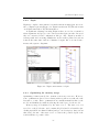
Usage example: Abstract queue
The specification language has a limit where a refinement becomes too complex and explicit. At some point the refined specification must become the
basis for implementation. This is the penultimate step in VDM, to stop
when the specification becomes appropriately concrete and implementation
is fairly straight forward.
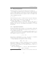
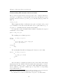
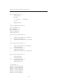
On to the specification language itself, we have an example of a abstract
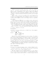
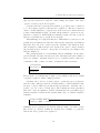
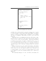
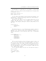
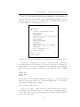
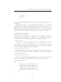
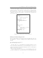
queue in Figure 2.1, gathered from [27]. This example shows some of the
main features in VDM-SL, such as types, state and operations. It is given
in the standardised ASCII notation.
The example has a state, TheQueue, which internally is given by the
variable q, which is a sequence of tokens. Sequences have an inherent ordering, unlike sets. There are three operations defined, which are like functions,
in that they specify valid operations. Each operation may include a pre- and
a post-condition. They can be used to implicitly describe what the operation
does.
5
Chapter 2. Background
types
Qelt = token;
Queue = seq of Qelt;
state TheQueue of
q : Queue
end
operations
ENQUEUE(e:Qelt)
ext wr q:Queue
post q = q~ ^ [e];
DEQUEUE()e:Qelt
ext wr q:Queue
pre q <> []
post q~ = [e] ^ q;
IS-EMPTY()r:bool
ext rd q:Queue
post r <=> (len q = 0)
Figure 2.1: A queue abstract type written in VDM-SL.
Here the DEQUEUE operation takes no arguments, but returns an element,
e. The ext wr specifies that the following variable is modified. DEQUEUE has
a pre-condition that the queue cannot be empty, i.e. the queue (q) is unequal
to the empty sequence []. The post-condition for DEQUEUE is
q~ = [e] ^ q
where the tilde (~) signifies the variable prior to the post-condition. The
brackets make a sequence of the variable e, and the hat (^) concatenates
the two sequences. I.e. the element e is the head of the queue before the
operation.
Specification language
We glimpsed at the specification language above. Actual produced specification papers are usually written in a mixture of textual and formal description. The textual part guides the reader on what the description describes
and how it is used. This section uses information from [13].
In addition to the types and operations sections in the example above,
VDM-SL also provides values and functions sections. All sections are not
required. The functions are true functions, and the values are fixed and
resemble constants in programming languages.
6
2.2 Selected specification languages
VDM is strongly typed, and the basic types are common sets of numbers,
such as boolean (bool), natural numbers (Nat), integers (int) and real
numbers (real). Additionally are the ‘character’ which is the VDM-SL
character set, and tokens. Tokens have minimal properties, and are a base
on which to expand in refinement. The Qelt type in the previous example
is a token.
All the common operators for the different types exist in VDM, such as
predicate logic, standard numeric, and comparison operators. See the postcondition for the IS-EMPTY operation for an example of the use of equivalence
and equality.
Compound types in VDM can be sets, sequences, maps, cartesian products, unions, and records. We have seen an example of sequences, and sets
has the expected operators, such as (proper) subset, union, and difference.
Additionally exist the finite subset operator. It is like a standard powerset
operator, only that all sets must be finite and the resulting set is also finite.
Records in VDM are like records in programming languages, in that they
consist of a collection of component fields. If the fields are named they can
be referred to with the ‘dot’-notation,
Person.phone
would refer to the phone field in the record value Person. Person might be
of type Person details:
Person :: name : Nametype
address : Addresstype
phone : Teltype
Function and operation arguments are given as values. To modify a
state the state variables must be given in the operation body with the ext
keyword as in the example in Figure 2.1. The ext must be followed by either
rd or wr signifying whether the state is only read, or if it is also written to
(modified). Functions are side-effect free like mathematical functions. VMD
additionally has support for anonymous functions, as in lambda calculus.
Finally VDM supports modules. Modules are defined in self-contained
units, with a clearly defined interface.
2.2.2
Z notation
Z notation is a specification language based on Zermelo-Fränkel set theory and propositional logic. The axiomatic (typed) set theory avoids some
paradoxes of naive set theory such as Russell’s paradox.
The usage example below is a partial specification of a phone number
directory. It is extracted from [13, Chapter 6]. As usual with Z specification the example is written with a mixture of a textual description and the
7
Chapter 2. Background
specification in Z notation. The text helps aid the reader and puts the specification in context. Integrated editors such as the editor in the Community
Z Tools project [28] has syntax and type checker built in.
Usage example: Phone number directory
The basic components of the phone number directory are names and numbers. They are defined as basic types:
[NAME , NUM ]
We define a schema to denote the state of the system. The directory
schema is named DIR and contains a function from names to numbers.
The function is defined as partial because not all possible names must have
an associated number. This function will work as a state for the system.
Generally schemas have both declarations and a predicate. The DIR schema
is only a declaration, but a possible predicate might be to restrict the number
of entries, such as #(dom dir ) < 1000.
DIR
dir : NAME →
7 NUM
Our first operation is to add an entry in the directory. It takes two
inputs, name? and no?. The question marks denotes that they are input
variables. The ∆DIR declaration is shorthand for [DIR, DIR 0 ]. This means
we have both the functions dir and dir 0 available to us in the operation.
Primed variables denotes the variable after the operation.
Add
∆DIR
name? : NAME
no? : NUM
dir 0 = dir ⊕ {name? 7→ no?}
The Add operation updates the directory function with the new mapping from name? to num?. The primed variable dir 0 is like the unprimed
variable except that the new mapping is added and overrides the previous mapping from name? if there existed one. We could add the predicate
name? ∈
/ dom dir to disallow adding an entry for a name that is already in
the directory.
Our other opertion looks up the number associated with a name. The
schema LookUp defines this behaviour. The declaration ΞDIR is like ∆DIR
8
2.2 Selected specification languages
with the additional predicate that the primed variables are identical to the
unprimed variables, i.e. the state is unchanged.
LookUp
ΞDIR
name? : NAME
no! : NUM
name? ∈ dom dir
no! = dir (name?)
The operation is defined so that the input name must be a part of the
domain of the dir -function. The output phone number is result of the application of dir on the input name. Both the predicates must be valid for
the schema to hold.
Language overview
The definitive texts for the Z notation are the reference manual by J.M.
Spivey [24] and the ISO 13568 standard [1]. Both texts are highly technical,
and so as not to delve too deep in the underlying syntax and semantics, the
information in this section is gathered from the books [13] and [20].
There are primarily two parts to the Z notation. The first is the actual
language itself, and the second is the standard mathematical toolkit. The
toolkit is created using the language itself, and contains many operators
that normally would be associated with the language, such as set operators
and function operators. The language itself governs the rules for identifiers,
references, declarations, etc. We will here not concern ourselves with the
difference, and rather give an overview of the Z notation on the whole. The
reader may refer to the reference manual [24] for further investigation.
Every variable in Z has a type. There are no subtypes. The only basic
type in Z is integer (Z). Natural numbers (N) are not a subtype of integers,
but rather a subset of integers with a predicate that restricts its range. So
the declaration x : N can be seen as shorthand for
{x : N | x ≥ 0}.
Set types are also called given types. The NAME and NUM types used
in the prior example are such types. They are basic sets, and their contents
are not defined. Convention states that these types are named as singular
nouns and written in capital letters. Several types can be defined at once:
[NAME , NUM ]
9
Chapter 2. Background
Enumerated types and recursive types are represented in Z as free types
or data types:
FreeType ::= Element1 | Element2 | . . . | Elementn
An element may either be a constant or a constructor. They must all be
distinct. The are often used to list possible messages in an abstract way.
For example: A switch type is a set of type SWITCH where the elements
may either be on or off . The data type definition is simply
SWITCH ::= on | off
The equivalent complete statement is
∀ x : SWITCH • x = on ∨ x = off
which is more complicated to write, especially when the number of distinct
members of the set increases. For a slightly more complex example, we can
use constructors to build a type for a binary tree that holds integers1 :
TREE ::= leaf | nodehhZ × TREE × TREE ii
Z has several compound types. The most common is sets, but Z also
provides cartesian products, bags and sequences. Sets are the basis for
the Z notation along with propositional logic. As such Z supports all the
common operators such as equality, subset, member, cardinality, union, and
intersection. Additionally is powerset, both finite and infinite. The powerset
is the set of all possible subsets. E.g. the powerset of the set of the numbers
zero and one is
P{0, 1} = {∅, {0}, {1}, {0, 1}}
Cartesian products in Z is defined with the same operator as ordinary
algebra, the cross (×) operator. Products may be referred to as tuples and
can be indexed with a conventional dot-notation (tuple.index ) to select the
components.
Sets cannot contain duplicates. Two compound types in Z that does
allow duplicates are bags and sequences. Bags are like sets where duplicates
are allowed and the number of duplicate elements are significant. They are
expressed in double square brackets ([[, ]]), and does not have to be finite in
size. Some of the common set operators have an equivalent version for bags:
−
membership (in), sub bag (v), union (]), difference (∪)
and cardinality
1
This is similar to how strongly typed functional languages such as Haskell defines
binary trees.
10
2.2 Selected specification languages
(#). Special operators for bags are count, scaling, and ‘items’. The items
operator creates a bag from a sequence.
Sequences in Z are represented in brackets (h, i). They can be restricted
to be non-empty sequences and injective sequences. Injective sequences
cannot contain duplicates. Sequences are in Z viewed as a functions from
positive natural numbers (N1 ). As such, all the function operators are applicative to sequences. Additionally are available sequence specific operators
such as concatenation (a), prefix, head, and tail.
Z has full support for algebraic function. This includes operators for both
partial and total functions, surjective and injective functions, and lambda
functions. E.g. the dom operator gives the domain for the function. Further description of functions is better described in course books for abstract
algebra such as [12], and in books specific for Z such as [13, Chapter 2.4]
and [20, Chapter 5].
The principal method for structuring and modularising a Z specification is schemas. We have already seen some schemas in the phone number
directory example. Schemas describes a set of variables whose values are
constrained. They consist of a name, declarations, and a predicate:
SchemaName
Declarations
Predicate
The predicate of a schema may be split over several lines, and are by default
conjoined together to make a single predicate.
Schemas can be used to describe states, operations, types, predicates,
and theorems. All types used in a schema must be either standard builtin types or types defined previously in the specification. Schemas can be
generic over one or more of their types. The schemas are then generalised
and can be used as templates. Generic schemas have the generalised types
written in square brackets in the schema name. E.g. a reusable database
template:
Database[KEY , DATA]
database : KEY →
7 DATA
Similarly, generic definitions are written without a name, but with a double
line at the top. Generic definitions can introduce a family of operations,
such as the head operation for sequences:
11
Chapter 2. Background
[X ]
head : seq1 X → X
∀ x : seq1 X • heads = s(1)
Variables ordinarily declared in a schema can be made globally by using an axiomatic definition. The axiomatic definitions have no name, only
declarations and a predicate. Not only can the axiomatic definition define
global variables and constants such as
array size : N
array size = 8
but also mathematical operators. As Z have not a built-in power operator,
we may define it ourselves as
↑
:N×N→N
∀p : Z • p ↑ 0 = 1
∀ n : Z1 • p ↑ n = p ∗ (p ↑ (n − 1))
and we may now use it the same way as we use the built-in operators.
As schemas form the backbone in structuring the Z specification, many
operations on schemas are well-defined. The operations disjunction, conjunction, negation, implication, equivalence, inclusion, quantification, hiding, projection, renaming, and sequential composition are all applicable.
This gives us the freedom and power to write statements such as
b Booking limit ∨ Overbooked
Ticket status =
to state that the aeroplane ticket status is either within the booking limit
(ergo purchasable) or that the aeroplane is overbooked. The complete calculus for the schema operations is too large to fit in this brief overview, but
both books [13, 20] contains a sizable section devoted to describing all the
mentioned operations.
We end with some Z conventions. As noted in the example in the previous section output variables and input variables are by convention marked
with an exclamation and question mark, respectively. Primed variables define the value of the variable after the operation. The shorthands ∆ and Ξ
are typically used on schemas that are included in other schemas. They respectively denote change and no-change of schema variables. For the simple
example in the previous section ΞDIR equates to the following schema:
12
2.3 Overview of tools for verification
dir
dir 0
dir 0 = dir
This convention helps readability in two ways: (1) The number of “lines” in
the schemas are kept to a minimum. (2) They serve as mnemonic helpers
to see the possible effect an operation has on states.
2.3
Overview of tools for verification
In this section we will not give overview of theorem helpers and automated
theorem provers. Focus will be on model checkers and process algebras.
Common is that they all work on a model of the system, and produces a
valid result on whether the model satisfies some correctness property.
2.3.1
Spin
Spin is a finite state model checker mainly developed by Gerard Holzmann.
It was designed for simulation and verification of network protocols and
distributed algorithms. The latest version of Spin is available for free at
http://www.spinroot.com/, both pre-compiled binaries for some common
operating systems, and complete source code. The definite text for Spin is
[14], on which this overview is based.
Models used in Spin are written in Promela. Promela describes a set
of processes that communicate via buffered or unbuffered channels, and via
shared variables. The total model is an asynchronous composition of the
processes2 . The complete state space for the model is explored on-the-fly.
Spin itself does not verify the model. In stead it generates an executable
C program that analyses the model. This means that only the necessary
analysis is compiled, and that all the compiler specific optimisations are
available to reduce the time needed for verification.
High memory usage is the main problem for explicit state model checkers
due to state explosion. Spin has several optimisations that combat this problem, such as partial order reduction, bit state hashing, coding the state as a
minimised deterministic automaton, and state vector compression. Bit state
hashing is notable because it is a lossy technique, i.e. it does not guarantee
2
Not that iIf synchronous communication is used in the model, then the transition
for a communication event is synchronised between the participants. I.e. both processes
transition at the same time, as would be in a synchronous composition.
13
Chapter 2. Background
that the entire state space is explored. However, this makes the verification run very fast, a very large part of the state space is actually explored,
and any violations that are found are true violations. All optimisations are
presented and explained in [14, Chapter 9].
Several forms for correctness specification of the model is supported: assertions, trace containment, progress cycles, acceptance-cycles, and propositional linear temporal logic. A never-claim is a special Promela process
that executes in lockstep with the model, and it is considered a correctness
violation if the never-claim ends or enters an acceptance-cycle. Correctness properties specified in propositional linear temporal logic is translated
into such a never-claim for verification. Finally it is possible to distinguish
between valid and invalid end-states. Invalid end-states are typically interpreted as deadlocked states.
The modelling language Promela resembles C in its syntax. Each statement in Promela defines a transition for the process. Non-determinism is introduced with statements very similar to Dijkstra’s Guarded Commands [7].
The only semantic difference is that the if and while statements in Promela
blocks if no guards are executable. Communication via both synchronous
and asynchronous channels use the operator similar to CSP, i.e. the question mark (?) for reception and the exclamation mark (!) for sending. The
channels in Promela are typed, and the channel descriptor may themselves
be sent over channels.
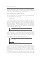
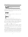
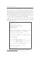
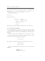
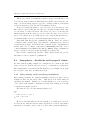
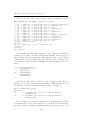
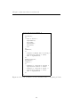
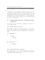
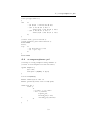
An example of a Promela model is given in Figure 2.2. The example is
from [3] and is a model of a server and two clients communicating over an
un-buffered channel. The clients request from the server, receives a reply
(and discards it), then terminates. The server is perpetually available as
given by the do statement. The label “end” in the server process says that
it is a valid end state.
2.3.2
FDR2 and ProBE
FDR2 and ProBE are commercial tools for verification and animation of
processes specified in CSP. Both tools are written by Formal Systems (Europe) Ltd. The information herein is gathered from [11, 21, 23]. A basic
introduction to CSP can be found in [23, Chapter 1].
Both tools are available for UNIX-type platforms; Linux, Solaris, OS X,
and FreeBSD. Additionally, ProBE is available for Windows. ProBE is available for download without charge, but FDR2 requires either a commercial
or academic licence.
The verification techniques in FDR2 are based on an operational semantics of CSP and on algebraic reduction techniques, and as such does not
explore the state space of the system explicitly. The system is built up
14
2.3 Overview of tools for verification
chan request = [0] of { byte };
chan reply
= [0] of { bool };
active proctype Server() {
byte client;
end:
do
:: request ? client ->
printf("Client %d\n", client);
reply ! true
od
}
active proctype Client0() {
request ! 0
reply ? _
}
active proctype Client1() {
request ! 1
reply ? _
}
Figure 2.2: Promela model of an elevator.
gradually, and several hierarchical compression techniques may be applied
to reduce the number of states visited. This enables FDR2 to check larger
systems. Compression techniques include normalisation, strong bisimulation, and τ -loop elimination. These must be specified on a process level in
the model.
FDR2 may check for determinism and refinement. The check for refinement uses the traces model, the stable failures model, and the failures/divergences model for CSP denotional semantics . This means that FDR2 is
not strictly a model checker, but rather a refinement checker. A process
model of an implementation is considered “correct” if it is a refinement of
a process model of its specification. Traces are events that processes can
observably engage in, and corresponds to language inclusion for automaton
theory.
Failures and divergences provide additional information. The failures
describe the events a process may refuse to engage in, and the divergences
describe when a process only engages in hidden events. Divergences can
be equated with the concept of livelock. A formal treatment can be found
in [21, Chapter 8], and a more informal treatment can be found in [23,
Chapter 4].
The actual input language for both tools is CSPM , the machine read-
15
Chapter 2. Background
able dialect of CSP. It combines the CSP process algebra with an expression
language with support for the idioms of CSP. The expression language is
functional, and inspired by the likes of Miranda and Haskell. It provides a
powerful type system, first-class functions, anonymous functions, lazy evaluation, and pattern matching. The operators in CSPM are designed to look
like the mathematical operators. E.g. the internal choice operator u is written as |~| and the sharing operator |[ C ]| is written as [|C|]. A complete
overview is given in [11, Appendix A] and [21, Appendix B].
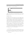
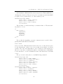
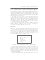
An excerpt from a model of multiplexed buffers, given in the FDR2
distribution3 , is shown in Figure 2.3. Removed from the model is faulty
transmission. The declared data types are abstract, and are the data that
the channels may receive.
datatype Tag = t1 | t2 | t3
datatype Data = d1 | d2
channel
channel
channel
channel
channel
left, right : Tag.Data
snd_mess, rcv_mess : Tag.Data
snd_ack, rcv_ack
: Tag
mess : Tag.Data
ack : Tag
SndMess = [] i:Tag @ (snd_mess.i ? x -> mess ! i.x -> SndMess)
RcvMess = mess ? i.x -> rcv_mess.i ! x -> RcvMess
SndAck = [] i:Tag @ (snd_ack.i -> ack ! i -> SndAck)
RcvAck = ack ? i -> rcv_ack.i -> RcvAck
Tx(i) = left.i ? x -> snd_mess.i ! x -> rcv_ack.i -> Tx(i)
Rx(i) = rcv_mess.i ? x -> right.i ! x -> snd_ack.i -> Rx(i)
Txs = ||| i:Tag @ Tx(i)
Rxs = ||| i:Tag @ Rx(i)
LHS = (Txs [|{|snd_mess, rcv_ack|}|]
(SndMess ||| RcvAck))\{|snd_mess, rcv_ack|}
RHS = (Rxs [|{|rcv_mess, snd_ack|}|]
(RcvMess ||| SndAck))\{|rcv_mess, snd_ack|}
System = (LHS [|{|mess, ack|}|] RHS)\{|mess,ack|}
Copy(i) = left.i ? x -> right.i ! x -> Copy(i)
Spec = ||| i:Tag @ Copy(i)
assert Spec [FD= System
Figure 2.3: Model of multiplexed buffers in CSPM (excerpt).
3
The file is named mbuff.csp can be found in the demo directory.
16
2.3 Overview of tools for verification
The system model is built up of simpler processes. The SndMess process says that the message request (snd_mess.i) is followed by an actual
transmission (mess ! i.x). Similar for the reception and acknowledgments.
The individual transmission (reception) processes Tx(i) (Rx(i)) governs the
events at a “higher level”, and these are composed to a single process Txs
(Rxs).
The total system is composed of a “right” and a “left” hand side, for the
transmission and reception respectively. In the composition of these processes the synchronisation alphabet is declared explicitly, and subsequently
hidden. The system process is composed similarly so that the only externally visible events for the system is the left and right channels. Finally
the model is checked to be a trace refinement of a process with precisely
these visible events.
2.3.3
LTSA
Labelled Transition System Analyser (LTSA) is a tool written by Jeff Magee
and Jeff Kramer. It is used and described in their book “Concurrency:
State Models & Java Programming” [17]. LTSA provides an integrated
environment for modelling and verification, and is written in Java. Thus it
is available for most desktop operating systems.
The input language for LTSA is FSP (Finite State Processes). FSP owes
much to CSP [16], and is as such fairly similar. The model is a synchronous
composition of smaller processes. Processes are described with how they
engage in global events. A process is defined as either a local process, or
as a process prefixed by an event. Non-determinism is introduced with a
choice operator (|), with a possible boolean guard (when).
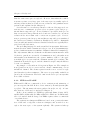
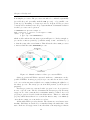
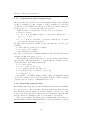
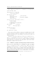
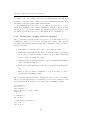
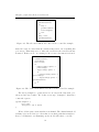
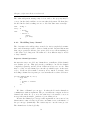
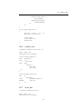
const Max = 3
range Int = 0..Max
SEMAPHORE(N=0) = SEMA[N],
SEMA[v:Int]
= ( signal -> SEMA[v+1]
| when(v>0) wait -> SEMA[v-1]
),
SEMA[Max+1]
= ERROR.
Figure 2.4: Semaphore model written in FSP
A simple semaphore model is given in Figure 2.4. It uses a global constant to set the maximum allowed value, and builds a range of possible values
that is used to index the local SEMA-processes. The down event is guarded
so that it is impossible to have a semaphore value less than zero.
The total model of a system is a single process. This process is created
17
Chapter 2. Background
from simpler processes. The processes can either be combined sequentially
(provided they end gracefully with the END process), or by parallel composition (||). Renaming of events is provided to help model the processes
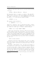
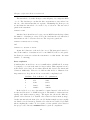
concisely and to facilitate reuse. E.g. a system that models mutual exclusion
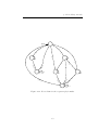
for three processes can be given as
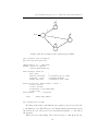
/* SEMAPHORE from previous example */
LOOP = (sema.wait -> critical -> sema.signal -> LOOP).
||SYS = ( p[1..3]:LOOP
|| {p[1..3]}::sema:SEMAPHORE(1)).
which would result in the automaton given in Figure 2.5. In the semaphore
process the events are prefixed (:) with the string “sema”, and shared (::)
so that they may take several names. This allows the three LOOP processes
to interact with the same SEMAPHORE process.
Figure 2.5: Mutual exclusion of three processes in LTSA.
Safety properties in LTSA is expressed with trace confinement, as also
possible in FDR2. A safety property is a process, and the model is considered correct if its automaton alphabet is contained withing the alphabet of
the safety process. The safety process is in FSP prefixed by the keyword
property.
Liveness properties are expressed with “progress” sets. A progress set
is a set of global event. The model satisfies the liveness property if it may
engage in one of the events in the set an infinite number of times. A second
progress property is described with an additional set. This is a conditional
property, which states that if one event in the first set may occur infinitely
often, then so must one event in the second set.
Additionally LTSA provides fluents. The fluents are an abstract state
machine. Each state is described by events that change the truth value of the
state. If the model engage in an event, then that event may trigger a fluent
18
2.4 Further specification languages and verification tools
to become either true or false. By using the abstract state machine one may
formulate temporal claims. LTSA supports propositional linear temporal
logic (PLTL) on fluents. PLTL can be used to formulate desired properties
of the system, both safety and liveness properties. E.g. the modeller may
now formulate a request-reply property such as [](P-><>Q) and verify that
a model satisfies this property:
assert SYS = [](msgsend -> <> msgreceive)
2.3.4
Choice of presented tool
The best tool for an introduction to formal verification of those given above
is Spin. This is especially true if the target audience is not well versed
in theoretical computer science. Spin sports an approachable description
language and a variety of ways to express correctness properties.
LTSA is a good introductory tool, but does not reach up to Spin due
to its use of a process algebra. The notion of a process algebra may be
an unusual concept for non-theorists, and likewise the process of building a
process as a synchronised parallel composition of other processes.
The final tool, FDR2, is very powerful, and has proven itself as very
useful for checking systems. E.g. it was used to expose and fix a flaw in the
Needham-Schroeder public-key protocol [15]. The reason FDR2 is not good
as an introductory tool to formal verification is that the only way to specify
correctness is through refinement. It seems that often it is desirable to
formulate simpler properties for the system, such as request-reply guarantee,
and not a model of the complete specification.
2.4
Further specification languages and verification tools
The formal methods presented in the previous sections are only a tiny minority of the available methods. Below is a small list of other tools that
might be of interest for further study. It is gathered from [30, 26, 29].
Alloy is a fairly light weight graphical tool. Aims to automate the checking
of Z-style specification in a way similar to model checkers.
B-Method is a specification language similar to Z, but lower level. It is
model checkable with the ProBE tool.
Java PathFinder is a model checker for Java programs. It started as a
translator from Java to Spin, but has now a custom made verification
engine to better handle the complexity of Java programs.
19
Chapter 2. Background
NuSMV is symbolic CTL and PLTL model checker. It is based on reduced
order binary decision trees, and can handle very large systems.
Petri-nets is a mathematical graphical notation. It may be used to analyse
concurrent systems.
UPPAAL is a model checker for timed automata.
20
Chapter 3
Theoretical foundation
Some more important concepts for formal methods, especially relevant for
model checking. The survey article by Merz [18] presents much of the same
theory, and is a good introductory text.
3.1
Automaton theory
The theory presented in this chapter is gathered from [19] and [25]. This
chapter is severly restricted to theory immediately relevant for temporal
logic model checking, but both references above contain further relevant
theory.
Automata operate on words, i.e. a sequence of symbols taken from a
given set named an alphabet. We let A be an alphabet throughout the
chapter. A word is denoted with juxtaposition of its letters such as
x = a1 a2 . . . an
where ai ∈ A, 1 ≤ i ≤ n. The set of all words in the alphabet is denoted by
A∗ .
A finite automaton is a tuple A = (Q, I , ∆, F ), where Q is a finite set
of states, I ⊆ Q is a set of initial states , ∆ ⊆ Q × A × Q is a transition
relation , and F ⊆ Q is a set of final states.
The automaton is deterministic if there is only one initial state, and
if for each pair (p, a) ∈ Q × A there is at most one state q ∈ Q such that
(p, a, q) ∈ ∆. Or, colloquially, if there are two or more transitions with from
a state with the same “label”. Else the automaton is non-deterministic. A
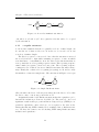
simple non-deterministic automaton is given in Figure 3.1.
The automaton is said to recognise the set of words ending with ab. We
denote the set recognised by the automaton as L(A). The word is recognised
by the automaton if the sequence of letters are a path of the automaton. A
path is a sequence c = (ei )1≤i≤n of consecutive edges (ei ∈ ∆, i.e. transitions
21
Chapter 3. Theoretical foundation
a
start
1
a
2
b
3
b
Figure 3.1: A non-deterministic automaton.
of A, where e1 ∈ I and en ∈ F . A recognised word is also said to be accepted
by the automaton.
3.1.1
ω-regular automata
So far we have assumed that the recognisable word are of finite length. As
A∗ was the set of finite words, now Aω is the set of ω-words over A. An
ω-word is of infinite length.
The Büchi acceptance of an ω-word δ is so that the automaton can read
the word from left to right while assuming a sequence of state in which
some final state occurs infinitely often. In other words, this means that at
some point in the word a repeating sequence starts. The repeating sequence
visits a final (“acceptance”) state at some point. The repeating sequence
continues forever. A Büchi automaton differs from a finite automaton in two
ways. Firstly the condition for recognising (accepting) words, and secondly
the initial set of states is a single state. The automaton in Figure 3.2 accepts
a,c
b,c
start
a
1
2
b
Figure 3.2: Simple Büchi-automata.
all words where the letter b follows (some time) after the letter a. Note that
the letter c may occur at any point in the word.
A significant result for the Büchi automata is that the equivalence problem and the inclusion problem are decidable [25, Theorem 2.3]. A second
significant result is that propositional linear temporal logic (PLTL) is expressively equivalent to first-order logic over ω-sequences. In other words,
this means that any PLTL formula can be translated into a Büchi automaton. We have the basis for model checking PLTL using Büchi automata
inclusion and equivalence.
22
3.2 Formal semantics
3.2
Formal semantics
All the information presented herein is gathered from [13, Chapter 7].
For a language, the syntax is the set of rules that governs if a statement
is allowed. The semantics concerns with the meaning behind statements,
and how the statement affects the program as a whole. An example is the
common assignment statement
i := i + 1;
which means that the variable i is different after the statement. Mathematically a variable holds the same value at all times, there are no before or
after states. The formula i = i + 1 is then clearly false.
Formal semantics takes into account states. There are three types of
notation; operational, denotional, and axiomatic. Axiomatic semantics, in
particular, can be used for both verification and derivation of code from
specifications.
3.2.1
Operational semantics
Operational semantics model execution of code as a sequence of states run
on an abstract machine. Each statement transforms the current state into a
new one until the execution ends.
The state is a function from a set of identifiers (variable names) to a set
of values. It can be seen as a set of (identifier, value)-tuples. Each construct
in the language is defined by a function
σ : Var → Val
that describes a transformation of a state. Var is the set of identifiers
(variable names), and Val the values held in the variables.
A state transformer is a map from one state to another:
M (P) : state → state
where P is a program, i.e. a sequence of functions. Convergence of the state
transformer to a final state r is written as M (P)(σ) ↓= r . Divergence is
written with upward-pointing arrow and signifies that the execution does
not terminate, M (P)(σ) ↑.
The assignment statement x := e can now be defined with substitution1 :
M (x := e)(σ) = σ [v (e)(q)/x ]
1
Substitution is represented by a forward slash; a/b means replacing b with the value
of a
23
Chapter 3. Theoretical foundation
where v (e)(σ) is the value of the expression e in state σ. The assignment
statement x := x + 1, with 3 as the current value of x , would then be represented with σ(x ) = 3, e = x + 1, and v (e)(σ) = 3 + 1 = 4.
A simple program such as
x := 1
x := x + 2
is then represented as
M (x := 1; x := x + 2)(σ)
= M (x := x + 2)(M (x := 1)(σ))
= M (x := x + 2)(σ[1/x ])
= σ [1 + 2/x ]
= σ[3/x ]
The final state is then the initial state with the value of x replaced by 3.
3.2.2
Denotional semantics
Denotional semantics also uses an abstract machine representation. It differs
to operational semantics in that how the constructs are actually executed
is abstracted away. I.e. there are no intermediate states, and execution is
functional.
The state σ is seen as representing the model of the storage location,
i.e. the values held in memory by the abstract machine. The environment
operation ρ associates an identifier with a location.
σ : location → value
ρ : id → location
The meaning of an identifier is then its corresponding storage location:
M : Enviroment
def
M [id ]ρ = ρ(id )
To find the actual value held at a specific location we define a function
contents:
contents : State
def
contents(loc)σ = σ(loc)
24
3.3 Temporal logic
We can now define the meaning for the expression id1 + id2 as
def
M [id1 + id2 ] =
let loc − id1 = M [loc − id1 ]ρ in
let loc − id2 = M [loc − id2 ]ρ in
contents(loc − id1 )ρ + contents(loc − id2 )ρ
3.2.3
Axiomatic semantics
Axiomatic semantics is based on the Hoare triple
{P }S {Q}
which says that if execution of S began in a state satisfying P , then it will
terminate in finite time in the state Q.
A way to prove code using axiomatic semantics is the technique involving weakest pre-conditions (wp). The technique seeks to find the set of all
pre-conditions to a statement S and a post-condition Q, wp(S )(Q). For example: wp(i := i + 1)(i ≤ 1) = (i ≤ 0). With a specified pre-condition P we
can then prove the statement S by checking that P satisfies the computed
weakest pre-conditions.
Proof partitioning helps in breaking down the proof into sizable chucks.
If the post-condition Q can be split into two components Q1 and Q2 , then
we can split the statements S into components S1 and S2 such that
{P }S1 {Q1 ∧ P2 }
{P2 }S2 {Q2 }
still satisfy the original post-condition Q. By utilising this we can semiautomatically extract code (S ) from e.g. Z specifications where pre- and
post-conditions are given.
3.3
Temporal logic
There are many classifications of temporal logic. These are well presented
in [9, Chapter 2], and this section is gathered from it. All temporal logics
are concerned with describing and reasoning about how truth values of assertions change over time. We will look at two temporal logics must used in
model checkers: PLTL and CTL. They are respectively linear and branching
time.
25
Chapter 3. Theoretical foundation
3.3.1
Propositional linear temporal logic
The basic temporal operators for propositional linear temporal logic (PLTL)
are Fp (“eventually p”), Gp (“always p”), Xp (“nexttime p”), and pUq
(“p until q”). The formulae are built up of atomic propositions, truth connectives (land , ∨, ¬ , etc.) and the temporal operators.
PLTL is defined on a linear-time structure M = (S , x , L) where
• S is a set of states
• x : N → S is an infinite sequence of states (also written as x =
(s0 , s1 , s2 , . . .), and
• L : S → P AP is a labelling of each state with the set of atomic
propositions (AP ) true at the state.
We may define the syntax of PLTL by the following rules: (p and q are
formulae)
1. each atomic proposition P is a formula
2. p ∧ q and ¬ p are formulae
3. pUq and Xp are formulae.
The other operators can be formulated with these rules. E.g. Fp abbreviates
(trueUp and Gp abbreviates ¬ G¬ p.
The semantics is defined with respect to the previously defined lineartime structure. The statement M , x |= p mean that the formula p is true
on the time-line x . It is defined inductively2 :
1. x |= p iff P ∈ L(s0 )
2. x |= p ∧ q iff x |= p and x |= q
3. x |= ¬ p iff it is not the case that x |= p
4. x |= (pUq) iff ∃ j (x j |= qand ∀ k < j (x k |= p))
5. x |= Xp iff x 1 |= p.
An example of a PLTL formulae is G(p ⇒ Fq). It intuitively means
“if p is true, q will be true at some subsequent moment”. This is a typical
“request-reply” property for communication protocols.
3.3.2
Branching temporal logic
In branching-time temporal logic the underlying time structure is an infinite
tree, as opposed to a linear structure. Each moment in the time structure
have many successor moments. To specify formulae on the tree two additional operators are introduced. They are branch quantifier: either A or E,
and they mean “for all futures” and “for some future” respectively.
There are two main representations for branching time temporal logic:
CTL and CTL* . CTL (Computational Tree Logic) is the simpler one and in
2
The notation x i is the suffix path si , si+1 , si+2 , . . ..
26
3.4 Finite state model checking
it a branch quantifier may only be followed by a single linear temporal operator (G, F, X, and U). CTL* allows for an arbitrary linear-time formula,
and can therefore be seen as a super-set or CTL and PLTL.
We will not give the syntax and semantics for CTL and CTL* , but they
can be found in [9, Section 4] and, with a slightly more practical explanation
in [5, Chapter 2].
3.4
Finite state model checking
Model checkers analyses a system with respect to a property expected to
hold for the system. We will only consider systems of finite state. This
section is gathered from [5], unless otherwise noted.
3.4.1
Model checking PLTL
Model checking PLTL formulae follows readily from the theory of Büchi automata and ω-runs. We know that the language accepted by PLTL formula
can be formulated as a Büchi automaton. This Büchi automaton may then
be checked together with the associated state machine (the system model).
Let φ be a PLTL formula, A the automaton symbolising the system
model, and Bα be a Büchi automaton that recognises precisely the executions
of α.
The idea for PLTL model checking is as follows, provided φ is a desirable
property of the system:
1. Construct an automaton B¬ φ from the negated formula
2. Generate the synchronised product of the two automata A ⊗ B¬ φ
3. Check if the language recognised by A ⊗ B¬ φ is empty.
Now the model checking problem of “does A |= φ” is reduced to an emptiness
check.
While the theory is fairly straight forward to here, the actual consequences are not. Translating a PLTL formula into an equivalent Büchi
automaton is not easy, and is the subject of considerable research. The
size complexity for the automaton is O(2|φ| ). The product A ⊗ B¬ φ has
size complexity O(|A| × |B¬ φ |). In other words, the size is exponentially
increasing. This may seem like a significant problem, but it is reduced by
the fact that PLTL formulae are generally fairly short.
At an implementation level, the PLTL model checker Spin generates
the B¬ φ explicitly [14]. The automaton is presented to the user who may
modify it. The algorithm in Spin works by executing the model automaton
in lock-step with the Büchi automaton. Only transitions allowed by the
Büchi automaton is explored. Infinite executions are handled by a nested
depth first search. The first search finds a finite run to an accepting state
27
Chapter 3. Theoretical foundation
and marks it, and the second search starts at successors of the marked state
and searches for a finite run that ends in the marked state3 . If a run exist,
then the language intersection is non-empty and the model does not satisfy
the formula.
3.4.2
Model checking CTL
Model checking CTL formula is presented in [6]. The algorithm is very
different from model checking PLTL. As there is no equivalence between
CTL and automata, the method operates on the formula itself.
The algorithm operates on the time structure M = (S , R, P ) in stages
to label the states of the graph. The CTL formula has length n. The first
stage processes all sub-formulae of length 1, the second all sub-formulae of
length 2, and so on. At the end of the last stage all sub-formulae, including
the complete formula, has been labelled on the states.
The labelling procedure must handle a minimum set of cases for formulae
forms: atomic formulae f , ¬ f1 , f1 ∧ f2 , AXf1 , EXf1 , A(f1 Uf2 ), and E(f1 Uf2 .
Any CTL formula can be reduced to use only these constructions.
A proof of the A(f1 Uf2 ) part of the algorithm is included in [6, Appendix 1]. The time complexity of the complete algorithm is O(|f | × (|S | +
|R|)) [6, Theorem 3.1].
3
An accepting ω-run must be the concatenation of a finite run and a repeating run
that enters an accepting state an infinite number to times.
28
Chapter 4
Spin introduction and
tutorial
This tutorial aims to be self-contained, and will as such repeat much from
earlier in this thesis, albeit in lesser detail. The aim for this tutorial is that
the reader should feel comfortable in approaching some common models.
The description of semaphores is gathered from [2, 3]. All the semaphore
examples appear in [8], with exception of the resource controller with priorities which is from [4]. It is encouraged to have a copy of the original
examples available, if possible.
Full listings for most models are included in Appendix A.
4.1
Language introduction
The description language for Spin is Promela. It describes a set of processes.
The processes can communicate using shared variables or by communication
channels1 . Its syntax is similar to programming languages such as C, but
with non-deterministic selection and looping constructions.
4.1.1
Processes
Processes in Promela is declared with the proctype keyword.
active [1] proctype Example () {
/* body */
}
If the process type is declared with the keyword active, as above, then
it is automatically created. The [1] is not needed, but replace 1 with the
1
Promelas communication channels are similar to CSP both in behaviour and syntax,
but can also be asynchronous.
29
Chapter 4. Spin introduction and tutorial
number of processes to create. Processes can be started explicitly with a
run statement:
run Example();
Each process that is running/active is given a unique identification number. This number is stored in each process’ local variable _pid, and a creator
can store this value in a pid variable by assigning the run command to a
variable:
pid child = run Example();
A process ends if it executes its final statement. It will be killed if it is
the process with the highest process id. This means that it will not be killed
until its children is.
The process types can take arguments. E.g. a process type that takes
one Boolean variable and two bytes:
proctype WithArguments(bool enable; byte alpha, beta) {
...
}
Arguments are separated by semicolons, unless they are of the same type,
then they are separate by a comma. A comma implies that the subsequent
name is of the same type as the previous.
The init process is a process that is always created first regardless of its
position in the source code. It is commonly used to initialise global variables
and to create other processes:
init {
/* initialise global variables */
/* create processes */
}
4.1.2
Variables
Variables in Promela has one of two scopes; either global or process local.
Global variables are naturally accessible to all processes. Local variables
can be declared at any point in a process, but are initialised at creation.
This means that there is no notion of scope within blocks of code. All local
variables used within a process should therefore be declared together at the
start.
proctype P () {
byte temp;
bool enabled = true;
/* only behaviour, no variable declarations */
}
30
4.1 Language introduction
A variable is initialised to 0 unless it is explicitly given a value. The
above variable temp is then initialised to 0, but enabled is initialised to
true.
Some basic variable types of Promela are bit, bool, byte, short, int,
and unsigned. These all behave as one would expect, except that unsigned
variables must have a specified with in bits. An unsigned variable stored in
four bits that is initialised to 3 is declared as
unsigned v : 4 = 3;
Additionally of interest are mtype and chan. The mtype variable type
holds symbolic names. The symbolic names must be declared in one or more
mtype declarations:
mtype = { syn, synack, ack, nak };
mtype = { msg };
Variables can be printed with the printf statement. Additionally can
the symbolic name of the mtype variables be printed with printm or with %e
in printf. I.e. printm(var) gives the same output as printf("%e",var).
Assignment of variables is such that the value of th variable on the left
of an equality sign (=) is replaced with the value of the evaluated right-hand
side. The right-hand side must be side-effect free. The statements var++
and var-- are shorthands for var=var+1 and var=var-1.
4.1.3
Channels
Channels are declared with the chan keyword and a special syntax. To
create a channel that holds 3 messages, where each message is an mtype and
a byte we write
chan link = [3] of {mtype, byte};
The channel is represented by a number, and this number is stored in the
variable link. The reference to a channel can then be sent over a channel if
so needed. However, a caveat is that the channel is ‘destroyed’ if the process
that created it is killed. It is an error to communicate over a non-existing
channel.
Sending and receiving on a channel is executed with the ! and ? operators. Following the example channel above, a process can send on a channel
by executing
link!msg,seqno
Then the message contains the symbolic name msg and the value of the
variable seqno. Receiving on a channel is symmetrical:
31
Chapter 4. Spin introduction and tutorial
link?msgtype,value
fetches a message from the channel and stores its contents in the variables
msgtype and value. The types of the variables must be compatible. A
receive statement on an empty channel is blocking, as is a send statement
on a full channel.
A channel that can hold one or more messages is called an asynchronous
channel. By declaring that a channel can hold zero messages it is a synchronous channel. Communication on a synchronous channel is such that
both the sender and the receiver execute their respective statements at the
same global state machine step. This means that no other statements may
be interleaved between them. Synchronous communication need no temporary storage, and as such saves on memory usage.
4.1.4
‘Executability’ and non-determinism
Each statement in a Promela model is subject to ‘executability’. A statement can either be executable or not. When several statements in the global
model are executable, then one of them is chosen non-deterministically. If no
statements are executable then the model has ended. However, the special
statement timeout becomes executable, and can work as a ‘way out’.
Assignments are always executable. Boolean expressions are executable
if they evaluate to true. A special case is the expression (1), which is always
true and always executable. The skip statement is synonymous with (1).
4.1.5
Selection, repetition and control statements
Local non-determinism is introduced with if and do statements:
if
:: var == 1 -> printf("equal one\n")
:: var > 0 -> printf("positive\n")
:: else -> /*statements*/
fi;
The first statement after a double colon (::) is called a guard. When a
process reaches an if statement it chooses non-deterministically between all
executable guards. If no guards are executable then the else is executable
if present. So with if var is equal to 1 our example will either print “equal
one” or “positive”. The else guard is not legal if one of the other guards is
a communication statement.
The do statement is a similar to the if statements, with the same syntax
and rules for non-determinism, but it loops forever. The break statements
exits the do statement an transfers control to the statement right after the
loop.
32
4.1 Language introduction
Promela includes a goto statement. A goto statement is an unconditional jump to a labelled statement. Statements can be labelled, and a goto
jumps to the specified label immediately. The labelled state is also called a
control state. The goto statements works so that the statement preceding
the goto is immediately followed by the labelled statement, there are no
interim states. This means these two fragments describe the same exact
behaviour:
L2:
a = 0;
goto L2;
b = 1;
a = 0;
b = 1;
4.1.6
Verification
Spin offers several verification methods. The most basic is the assertion.
Assertions state simple safety properties, and are always executable. The
assert statement can take any valid Promela statement as its argument, and
if the argument is not executable, then the assertion is flagged as violated.
A common verification property is ‘no deadlocks’. Promela and Spin
does not use the term deadlock. The closest term is ‘invalid end states’.
Models in Promela are allowed to end. When the model has stopped, either
from a successful ending or a deadlock, the state of the individual processes
is marked as either valid (good) or invalid (bad). States in the processes
that are valid are either the state after the final statement, or states that
have labels that starts with end.
Arbitrary correctness properties can be formulated with propositional
linear temporal logic (LTL). LTL formulae specify behaviour in linear time.
The usual logical operators are not changed, e.g. implication (->), conjunction (&&) and negation (!). Five new operators are introduced, all temporal:
Operator
[]
<>
X
U
V
Function
Always
Eventually
Next
Strong until
Dual of U
Arity
Unary
Unary
Unary
Binary
Binary
The [], <>, and X operators are unary. U and V are binary operators.
A statement []p is true in any state where p is true and p is also true for
all following states. Similarly for the <> operator; <>p is true if p is true in
some future state. Xp is true if p is true in the next state.
33
Chapter 4. Spin introduction and tutorial
The strong until-operator is defined as such: p U q is true for a given
state if q is true, or if p is true in the state and is true in all future states until
q becomes true. Note that since this is a strong until operator q must eventually become true. The operator V is dual to U, i.e. p V q <-> !(!p U !q).
Spin can also verify by searching for non-progress cycles, trace-violations,
and directly written never-claims. We will only touch on never-claims as LTL
formulae are translated into never-claims for verification.
4.2
General Spin usage
A Promela model is a state machine, and each statement is a transition.
Non-determinism is then the choice between possible out-going transitions.
The state machine is the automaton product between all processes. However,
the automaton product is handled by Spin, and the modeller only need to
worry about the synchronisation between the individual processes.
While modelling the system it is often useful to use simulation to get
an impression that the model behaves as it should. Interactive simulation
(spin -i model.pml) enables the modeller to explicitly choose between possible transitions. This might be helpful in steering the simulation to a specific
subset, to examine a particular behaviour of the model.
4.2.1
Verifying a model
Spin does not actually verify a model, but rather generates source code for
a one. The Promela model is analysed and Spin builds a verifier that does
the verification.
A normal procedure for verification is as follows:
1. spin -a model.pml: Executing Spin with the argument -a will parse
the Promela model in model.pml and generate C source code files for
a verifier that will check the model. The C source code is put in the
file pan.c.
2. cc -o pan pan.c: The C program generated by Spin is compiled into
the program pan.
3. ./pan: Run pan to execute the verifier. The status given after completion tells if the verification was successful or not. If not, then a trail
to the violation is generated.
4. ./pan -r or spin -t -p model.pml: Execute the model with the
trail to violation so as to view the trail in human readable format.
34
4.2 General Spin usage
4.2.2
Xspin
Xspin is a complete environment for formal verification using Spin. A screenshot of Xspin is given in Figure 4.1. Xspin is written in Tcl/Tk and is runs
on all platforms with a Tcl/Tk distribution.
A significant advantage in using Xspin is that one need not remember
what arguments and pre-processor directives that Spin can take. In stead
they are exctracted from configuration dialogs. Also, Xspin is useful for
viewing trails and executing simulations as the trail is printed in various
forms at the same time, such as columnated output, list of executed statements, and sequence diagrams.
Figure 4.1: Xspin environment for Spin.
4.2.3
Optimising for memory usage
Optimising for time is rarely done, as memory is a scarcer resource. However,
some optimisations directed at reducing memory will as a result also take
less time to verify. These optimisations are usually manual tweaks for the
model, and ultimately results in reducing the state space for the model.
Memory usage is dominated by the state vector. The state vector is
stored for each global state, and contains all global and local variables (including asynchronous channel buffers) and process descriptors. Any actions
that reduce the size of the state vector or reduces the possible depth of the
search will have a positive effect.
35
Chapter 4. Spin introduction and tutorial
Whenever possible, deterministic sequences in processes should be enclosed in a d_step declaration. This helps the partial order reduction technique. A caveat with d_step as opposed to atomic is that no statements
except the first may block, else the determinism is broken.
A tip for reducing the number of processes is to drop the init process.
The init process is really just an active process that is started first. Any
processes may be started from an other active process, so by moving the
run-statements from the init process we reduce the state vector by four
bytes. Note that a more powerful pre-processor such as m4 enables us to
programmatically create processes with arguments as active processes.
Optionally Spin has several optimisations built-in. These are enabled
or disabled with compiler flags. Generally the optimisations are directed
towards memory usage, and will increase verification time. Optimisations
include state vector collapse compression (-DCOLLAPSE) and state vector
coding as minimised deterministic automaton (-DMA=n). Many optimisations
may be combined, but the benefits are highly problem specific.
The reference manual [14] and Theo Ruys’ Ph.D. thesis [22] provide
information on more advanced optimisations.
4.3
Semaphores—deadlocks and temporal claims
We start with modelling semaphores. Semaphores are common and their
usage error prone. In short, they are a very good candidate for verification.
The examples have been taken from The Little Book of Semaphores [8], with
the exception of the last one which is from [4].
4.3.1
Busy waiting, weak and strong semaphores
Busy waiting resembles the wait()/notifyAll() pattern from Java. Strong
semaphores have an associated queue. This queue is modelled using an
asynchronous channel. Waiting on a weak semaphore does not preserve
order. All a weak semaphore guarantees is that some waiting process will
be awaken at a signal-operation.
The naı̈ve model of a busy waiting semaphore is
wait:
if
:: atomic { sem > 0; sem-- }
:: else -> goto wait
fi
However, this will make the model actually loop, which is not needed.
A better model, that uses the fact that a Promela process is blocked until a
statement is executable, removes the loop. The wait-operation will then be
36
4.3 Semaphores—deadlocks and temporal claims
atomic { sem > 0; sem-- }
Clearly busy waiting semaphores generate smaller models. However,
they are not applicable if either (a) knowing how many is waiting is needed,
or (b) order is important. Some knowledge can be extracted by searching
for fairness. Processes that waits will be executable an infinite number of
times—as a signal will “notify” all waiting processes—and fairness says that
processes that are executable an infinite number of times will eventually
execute.
Any examples that use semaphores will use the simplified busy-wait
semaphores, unless otherwise specified. The wait and signal operations are
defined as pre-processor macros:
#define wait(s) atomic { s > 0; sem-- }
#define signal(s) s++
4.3.2
Simple mutual exclusion
Starting very simple we have two processes, each with a critical section
protected by a common semaphore. The processes behave the same, and so
only one proctype definition is needed:
proctype P () {
atomic {sema > 0; sema--};
/*critical section*/
sema++
}
The variable sema is a global short variable initialised to 1. We create
both processes by declaring the proctype definition to be active, and indicate
how many we start in brackets:
active [2] proctype P () {...}
To verify that the two processes cannot both be in their critical section
at the same time we have to add something to either the model or the code.
One way to check is to replace the critical section with an assertion. The
assertion can check that the sema variable is equal to zero. A value of zero
means that the semaphore has been decremented only once.
short sema = 1
active [2] proctype P ()
{
atomic {sema > 0; sema--};
assert(sema == 0);
sema++
}
37
Chapter 4. Spin introduction and tutorial
The complete model is given above. Verifying the model using spin we
get the following output:
(Spin Version 5.2.0 -- 2 May 2009)
+ Partial Order Reduction
Full statespace search for:
never claim
assertion violations
cycle checks
invalid end states
- (none specified)
+
- (disabled by -DSAFETY)
+
State-vector 20 byte, depth reached 8, errors: 0
15 states, stored
1 states, matched
16 transitions (= stored+matched)
0 atomic steps
hash conflicts:
0 (resolved)
4.653
memory usage (Mbyte)
unreached in proctype P
(0 of 6 states)
pan: elapsed time 0 seconds
As we can see the model has no violations. Specifically, the model will
not have an assertion violation, nor will it have a deadlock. However, if we
make the test-and-set part of the semaphore non-atomic, there will be an
assertion violation.
Assertions only holds at a single state. If in stead we wanted the proposition to be an invariant2 for the model we could introduce a new process
that monitors the rest of the model. We could also formulate the invariant
using temporal logic. Both these approaches will be used in the SearchInsert-Delete example in subsection 4.3.5.
4.3.3
Childcare example and interpreting invalid end states
From section 7.2 of The Little Book of Semaphores we have an example
where a room must have at least one adult per three children. If we allow
signalling an arbitrary amount, i.e. increase the semaphore with any number
higher than 0, not just 1, then a very simple solution exists. This solution
has one drawback, in that a child may wait even though an adult is inside.
This happens when an adult tries to leave, but must wait for some children.
2
An invariant is a logical proposition that holds for every state in the model.
38
4.3 Semaphores—deadlocks and temporal claims
The first thing we do is make macros for our semaphore operations. This
way the code is closer to what we mean; wait(sem) is more descriptive than
atomic{sem>0; sem--}.
#define wait(s) atomic{s>0; s--}
#define signal(s,n) s=s+n
Note here that we allow signal to take an amount as an argument. Some
implementation of semaphores may support this. If not, then a mutex protected loop will do the same job.
The model for the child process is even simpler than in the previous
example: The child enters the room by waiting at the door, then plays
indefinitely. The semaphore multiplex counts how many children are in
the room.
proctype Child () {
wait(multiplex);
/*play*/
}
The adult is the first one to enter. The multiplex semaphore is therefore
initialised to zero. When the adult enters he signals the semaphore by 3.
When the adult wants to leave he waits three times. The code is still fairly
simple:
proctype Adult () {
signal(multiplex, 3);
/*supervise*/
wait(multiplex);
wait(multiplex);
wait(multiplex);
}
We are now faced with the problem of deciding how many of each process
type we need for the complete model. We want the number of processes to
be as small as possible, but enough to find all possible flaws in the model.
Obviously we need three or more children, else an adult may never leave.
Since the adults influence each other, we need at least two adults. We decide
on two adults and three children.
Now we verify the childcare model so far. We restrict the checker to
safety properties.
spin -a childcare.pml
cc -DSAFETY -o pan pan.c
./pan
39
Chapter 4. Spin introduction and tutorial
We have an error. Spin tells us that we are in an invalid end state.
Inspecting the trace by running ./pan -r we see this:
1: proc 1 (Adult) line 14 "childcare.pml" (state 1) [multiplex = (multiplex+3)]
2: proc 4 (Child) line 23 "childcare.pml" (state 3) [((multiplex>0))]
3: proc 4 (Adult) line
0 "childcare.pml" (state 0) [-end-]
4: proc 3 (Child) line 23 "childcare.pml" (state 3) [((multiplex>0))]
5: proc 3 (Adult) line
0 "childcare.pml" (state 0) [-end-]
6: proc 2 (Child) line 23 "childcare.pml" (state 3) [((multiplex>0))]
7: proc 2 (Adult) line
0 "childcare.pml" (state 0) [-end-]
8: proc 0 (Adult) line 14 "childcare.pml" (state 1) [multiplex = (multiplex+3)]
9: proc 1 (Adult) line 16 "childcare.pml" (state 4) [((multiplex>0))]
10: proc 1 (Adult) line 17 "childcare.pml" (state 7) [((multiplex>0))]
11: proc 1 (Adult) line 18 "childcare.pml" (state 10) [((multiplex>0))]
12: proc 1 (Adult) line
0 "childcare.pml" (state 0) [-end-]
spin: trail ends after 12 steps
#processes 1:
12: proc 0 (Adult) line 16 (state 4) (invalid end state)
((multiplex>0))
global vars:
byte
multiplex: 0
It seems that the last adult is waiting to leave. This is not unwanted
behaviour for us. There are three children inside playing, and it is not bad
that an adult must supervise them. This indicates that we have missed
something in our model, namely that some states are fine to always be in,
even at the end. We add this by labelling the wait-statements as an endstates.
active [2] proctype Adult () {
signal(multiplex, 3);
/*supervise*/
end:
wait(multiplex);
wait(multiplex);
wait(multiplex)
}
Confident we have fixed our model, we try verifying it again. But we
still have errors. And it is still an invalid endstate. This time it is in both
the adult processes, as seen in the truncated output of ./pan -r:
spin: trail ends after 11 steps
#processes 2:
11:
proc 0 (Adult) line
((multiplex>0))
11:
proc 1 (Adult) line
((multiplex>0))
17 (state
7) (invalid end state)
18 (state 10) (invalid end state)
We obviously have discovered a flaw in the model. What happens is that
both adults want to leave, and are allowed to do it. However, they interleave
the wait-operations, resulting in a situation where the semaphore is zero, but
40
4.3 Semaphores—deadlocks and temporal claims
they both wait. Though it is possible to see this problem without checking
the model, we now have proof.
The solution is to make the wait-operations atomic, as said in section
7.2.2 of The Little Book of Semaphores. We protect the wait-operations
with a mutex:
active [2] proctype Adult () {
signal(multiplex, 3);
/*supervise*/
wait(mutex);
end1:
wait(multiplex);
end2:
wait(multiplex);
end3:
wait(multiplex);
signal(mutex, 1)
}
The mutex variable is initialised to 1. We reuse the semaphore operations. We label each wait-operation except on the mutex as acceptable
end-states. We can do this because we know now that only one adult will
start leaving at the time, and an adult must stay inside while there are
children. Now our model should be correct, and we expect no errors in the
verification. We recompile and run pan:
pan: invalid end state (at depth 12)
pan: wrote childcare_fix.pml.trail
There are still errors. Inspecting the trace we see that a child is waiting
to enter. We have found a flaw in our model again, except this time it is
not our fault. Our scheme does not guarantee that a child must be able to
enter.
To see if this is the only error we run ./pan -c0 to find all verification
errors. There are 13 runs to errors. That is a bit too much to inspect one
by one, so we try to remove some of them. We know that a child can enter
and leave at any time, but we have only modelled the first part. Allowing
the child to also leave we get the following child process:
active [3] proctype Child ()
{
wait(multiplex);
/*play*/
signal(multiplex,1);
}
This reduces the number of errors to 7, which is more manageable. To
produce the actual traces we run ./pan -c0 -e. The first argument tells
the verifier to find all errors, the second argument writes each trace to error
41
Chapter 4. Spin introduction and tutorial
to own file. We can examine each trace by running spin -tX with X as
a number between 1 and 7. There are several arguments that give more
information, such as -p that prints all statements.
By examining the seven traces we see that in all of them one or more
children are waiting to enter. This is a limitation with the solution we have
chosen, and to overcome the limitation a different solution is required. Such
a solution is given in section 7.2.6 of The Little Book of Semaphores.
4.3.4
Room party example and state explosion
The room party problem appears in section 7.3 of The Little Book of
Semaphores. There are two actors; students and a Dean. There is only
one Dean, but arbitrary many students. The constraints of the problem are
described as such:
1. Any number of students can be in a room at the same time.
2. The Dean of Students can only enter a room if there are no students in
the room (to conduct a search) or if there are more than 50 students
in the room (to break up the party).
3. While the Dean of Students is in the room, no additional students may
enter, but students may leave.
4. The Dean of Students may not leave the room until all students have
left.
5. There is only one Dean of Students, so you do not have to enforce
exclusion among multiple deans.
The presented solution uses three semaphores and a scoreboard pattern.
The scoreboard pattern is a set of variables protected by a semaphore. Our
global variables in Promela code becomes a direct translation of this:
/* scoreboard */
byte mutex = 1;
short students = 0;
mtype = {not_here, waiting, inside};
mtype dean;
/* turnstile */
byte turn = 1;
/* rendezvouses; semaphores */
byte clear = 0;
byte lieIn = 0;
42
4.3 Semaphores—deadlocks and temporal claims
The code for the Dean and a student is given in Figure 4.2 and Figure 4.3,
respectively. Some of the details of why this particular semaphore pattern
works is not the focus here, as we will focus on checking that this model
actually fulfils the constraints given above.
active proctype Dean ()
{
wait(mutex);
if
:: students > 0 && students < MAX ->
dean = waiting;
signal(mutex);
wait(lieIn) /*get mutex from student*/
:: students >= MAX ->
dean = inside;
printf("break up\n");
wait(turn);
signal(mutex);
wait(clear); /*mutex from student*/
signal(turn)
:: else -> /*students == 0*/
printf("search\n")
fi;
dean = not_here;
signal(mutex);
}
Figure 4.2: Process declaration for the Dean in the room party problem
Checking for 50 students is probably too much. Since we do not know
how many students are necessary, we use a macro in its place. We make two
simple macros, one for the maximum allowed students at a party (MAX),
and one for the total number of student processes (N). The macro for MAX
is
#ifndef MAX
#define MAX 2
#endif
and the macro for N is similar. This macro allows us to override the default
when we generate the verifier. To override the MAX value to 3 we generate
the verifier by running the following:
spin -a -DMAX=3 roomparty.pml
Now we are ready to verify our model. Our verification properties are
very simple. We want the model to be deadlock-free, and that all parts of
our model is visited. In Promela/Spin terms we want no invalid end states,
and no unreached states.
43
Chapter 4. Spin introduction and tutorial
active [N] proctype Student ()
{
wait(mutex);
if
:: dean == inside ->
signal(mutex);
wait(turn);
signal(turn);
wait(mutex)
:: else
fi;
students++;
if
:: students == MAX && dean == waiting ->
signal(lieIn) /*mutex to dean*/
:: else -> signal(mutex);
fi;
printf("party\n");
wait(mutex);
students--;
if
:: students == 0 && dean == waiting ->
signal(lieIn) /*mutex to dean*/
:: students == 0 && dean == inside ->
signal(clear) /*mutex to dean*/
:: else -> signal(mutex)
fi
}
Figure 4.3: Process declaration for the students in the room party problem
44
4.3 Semaphores—deadlocks and temporal claims
Our defaults for MAX and N is 2 and 3 respectively. This is sufficient for
checking the behaviour. However, if we choose parameters such that MAX
is equal to N we get unreached code. The verifier reports:
unreached in proctype Student
line 55, state 5, "mutex = (mutex+1)"
line 56, state 8, "((turn>0))"
line 57, state 9, "turn = (turn+1)"
(3 of 36 states)
The relevant code in the student process starts at line 55. The surrounding chuck of code is:
if
:: dean == inside ->
signal(mutex);
wait(turn);
signal(turn);
wait(mutex)
:: else
fi;
We see that the signalling operation on mutex is never reached. Subsequently this means that the statement
dean == inside
is never executed. This statement is reached, however, because it is an option
for the if-statement. Spin does not report this as an explicit correctness
violation. We can reason that this is correct behaviour, as the Dean is not
allowed to enter the room unless the number of students is more than MAX.
So the unreached code here is harmless, in the sense that the model is still
correct.
We get even more unreached code if MAX is larger than N:
unreached in proctype Dean
line 34, state 11, "dean = inside"
line 35, state 12, "printf(’break up\n’)"
line 36, state 15, "((turn>0))"
line 37, state 16, "mutex = (mutex+1)"
line 38, state 19, "((clear>0))"
line 39, state 20, "turn = (turn+1)"
(6 of 27 states)
unreached in proctype Student
line 55, state 5, "mutex = (mutex+1)"
line 56, state 8, "((turn>0))"
line 57, state 9, "turn = (turn+1)"
line 64, state 18, "lieIn = (lieIn+1)"
line 74, state 31, "clear = (clear+1)"
(5 of 36 states)
45
Chapter 4. Spin introduction and tutorial
The unreached code in the Dean process is all party of a contiguous chuck
of code. The Student process has the three statements we saw earlier, but
also two other statements that are separate. Examining the Dean process
we find that the unreached code is the body of selection. The associated
guard is the statement
students >= MAX
which we know should never be true, as now MAX is strictly larger than
the number of Student processes, N. For the Students the new unreached
statements are also bodies in selections. The respective guards are
students == MAX && dean == waiting
and
students == 0 && dean == inside
Again, the behaviour of the model is correct. The first guard cannot be
true as the number of students never become MAX. For the second guard,
the Dean process never reaches the statement to set his status—the dean
variable—to waiting.
State explosion
Confident that our model is correct for small values of MAX and N, we may
be tempted to see if it is the same for larger values. This temptation is not
well founded, as we have chosen values that should describe the functional
behaviour sufficiently. However, we will use this model to illustrate how
important it is to keep the model at a reasonable complexity level.
Students
2
3
4
5
6
P.O. reduction
215
976
4580
24164
144867
No optimisation
352
2086
11875
70077
446370
In the table above you see the number of visited states for the model as
we increase N from 2 to 6. MAX is kept at 2. The number of states increase
rapidly, and with it memory usage. The figure also shows the difference
partial order reduction does. Partial order reduction reduces memory usage,
but the amount varies from model to model. In this example we save roughly
two-thirds of needed memory. Partial order reduction is enabled by default
when compiling the verifier. To force Spin to not use partial order reduction
the pre-processor directive NOREDUCE must be given at compilation:
46
4.3 Semaphores—deadlocks and temporal claims
cc -DNOREDUCE -o pan pan.c
State space explosion is a significant problem, and reducing the amount
of memory needed for verification should be a top priority. The time needed
by verification is of lesser importance.
Optimising for time usually means restricting the compiled verifier to
only the types of properties to be checked, such as SAFETY and NOCLAIM. By
modifying the model to be targeted by a specific property may also improve
the efficiency of the verifier.
Many of the optimisations available in Spin focuses on reducing memory requirements. Of note are partial order reduction, state vector collapse
compression, hash-compact compression, and storing the state as a minimised deterministic finite automaton (DFA). All of these preserve the state
space, and no states are lost. However, all of them increase the time needed,
some more than others. For example, Minimised DFA will greatly reduce the
memory requirement, often by several orders of magnitude. It will, however,
greatly increase the needed time, maybe also by orders of magnitude.
In short, optimisations should for the lesser experienced be only be applied when absolutely needed. Reducing the complexity of the model is
always the first step, and will both reduce both memory and time needed,
but additionally make the traces more concise and easier to read.
4.3.5
Search-Insert-Delete example and LTL formulae
As a last example from The Little Book of Semaphoreswe examine the
Search-Insert-Delete problem from section 6.1. The given solution uses
a ‘Lightswitch’-pattern that allows multiple entities to enter on the same
semaphore. The first that enters will wait on the semaphore, and the last
that leaves will signal the semaphore. This is analogous to using a light
switch, hence the name. It is given in section 4.2.2 of The Little Book of
Semaphores.
The problem itself it fairly straight forward. We have Search, Insert,
and Delete processes. The original problem specified that they operated on
a linked list. We are only interested in how access is governed, so we denote
it simply by a ‘critical section’.
We restrict ourselves to only model two of each process. Any more would
not yield further knowledge, fewer would not be feasible as we are interested
in how each process type interact with others and it self. The Promela
code for the Lightswitch-pattern is given in Figure 4.4, and the code for the
processes are given in Figure 4.5 together with the variables.
47
Chapter 4. Spin introduction and tutorial
typedef Light {
byte count = 0;
byte mutex = 1; /*semaphore*/
}
inline lightLock(L, S) {
wait(L.mutex);
L.count++;
if
:: L.count == 1 -> wait(S)
:: else
fi;
signal(L.mutex)
}
inline lightUnlock(L, S) {
wait(L.mutex);
L.count--;
if
:: L.count == 0 -> signal(S)
:: else
fi;
signal(L.mutex)
}
Figure 4.4: Lightswitch-pattern in Promela
48
4.3 Semaphores—deadlocks and temporal claims
byte insertMutex = 1;
byte noSearcher = 1;
byte noInserter = 1;
Light searchSwitch;
Light insertSwitch;
active [2] proctype Searcher ()
{
lightLock(searchSwitch, noSearcher);
crit:
/* critical section */
lightUnlock(searchSwitch, noSearcher)
}
active [2] proctype Inserter ()
{
lightLock(insertSwitch, noInserter);
wait(insertMutex);
crit:
/* critical section */
signal(insertMutex);
lightUnlock(insertSwitch, noInserter)
}
active [2] proctype Deleter ()
{
wait(noSearcher);
wait(noInserter);
crit:
/* critical section */
signal(noInserter);
signal(noSearcher)
}
Figure 4.5: Variables and processes for the Search-Insert-Delete problem.
49
Chapter 4. Spin introduction and tutorial
Understanding LTL formulae and never-claims
The problem description has several properties. One of them is that there
can only be one Insert process at the time. If we denote the Insert processes
in theirs critical sections as i_1 and i_2, we can write this proposition in
LTL3 as
!<>(i_1 /\ i_2)
This formula says that for all runs it is not the case that both i_1 and
i_2 eventually become true at the same time. We recognise this as a ‘good’
property, i.e. something that the system should satisfy.
To verify that our model satisfies this formula we translate the negated
formula into a never-claim:
spin -f ’<>(i_1 /\ i_2)’
The resulting never-claim is given as
never {
/* <>(i_1 /\ i_2) */
T0_init:
if
:: ((i_1) && (i_2)) -> goto accept_all
:: (1) -> goto T0_init
fi;
accept_all:
skip
}
We can simplify this without changing the behaviour of the claim.
never {
/* <>(i_1 /\ i_2) */
do
:: (i_1 && i_2) -> break
:: true
od
}
Our reasoning for rewriting it is that it removes the unnecessary skipstatement at the end, which would add a final, unnecessary state to a trace.
Additionally it makes it easy to extend the claim with similar statements.
Say we wanted to check the formula <>p \/ <>q. Then a corresponding
never-claim would be4 :
3
LTL is also referred to as PLTL, PTL and LTL. Its full name is Propositional Linear
Temporal Logic. Spin uses the name LTL, and so will we in this tutorial.
4
Note that there are several never-claims that corresponds to each LTL formula.
50
4.3 Semaphores—deadlocks and temporal claims
never {
/* <>p \/ <>q */
do
:: p -> break
:: q -> break
:: true
od
}
So we see that it is identical to the previous one, with the addition of a new
alternative.
Our formula !<>(i_1 /\ i_2) essentially says that (i_1 /\ i_2) is an
invariant for our system. An invariant is a proposition that holds for all
states of all runs of the system. In fact, duality for the ¡¿ and [] operators in
LTL gives that our formula is equivalent to []!(i_1 /\ i_2). This formula
says that for all states it is not the case that i_1 and i_2 is both true.
Invariants for the model
We have already established how to check for not two Insert process in the
critical section at the same time. The Delete processes have an identical
constraint, and the invariant is equivalent to the Insert invariant:
$!(d_1 /\ d_2)$
A Delete process have an additional property, namely that no Search
processes can execute concurrently with it. I.e. if a Delete process is in
its critical section, then no Search processes are allowed into their critical
sections. We can formulate this as an invariant:
!((d_1 \/ d_2) /\ (s_1 \/ s_2)
The final invariant for the model is equivalent to the previous. It states
that a Delete process and an Insert process should not both be in the critical
section at the same time:
!((d_1 \/ d_2) /\ (i_1 \/ i_2)
We can now include all our invariants into the model, and check them
all at the same time. The invariants is checked by a monitor process:
active proctype Monitor ()
{
end:
if
:: (i_1 && i_2) -> assert(!(i_1 && i_2))
:: (d_1 && d_2) -> assert(!(d_1 && d_2))
:: ((s_1 || s_2) && (d_1 || d_2)) ->
assert(!((s_1 || s_2) && (d_1 || d_2)))
:: ((d_1 || d_2) && (i_1 || i_2)) ->
assert(!((d_1 || d_2) && (i_1 || i_2)))
fi;
}
51
Chapter 4. Spin introduction and tutorial
The negation of each invariant guards an assert-statement on the invariant.
This works as the guards are only executable when the invariant is violated.
Violating a property as sign of correct behaviour
The final two properties are not invariants. The first states that two (or
more) Search processes can be in their respective critical sections at the
same time. On might be tempted to formulate this as <>(s_1 /\ s_2),
i.e. that eventually both Search processes are in critical section an the same
time. However, this is wrong because LTL formulae describes all runs. Here
this would mean that for all runs both Search processes would be in the
critical section, when it should only be so for one or more runs.
We overcome this by realising that we can view a property violation as
a good thing. Say we have the invariant !p. The invariant says that for
all runs it is never the case p becomes false. If this invariant is violated,
then it means that in one or more runs p eventually becomes true. We have
found a way to check that something can happen in some runs, without the
restriction that it must happen in all runs.
To find if two Search processes can execute their critical sections concurrently we then have the LTL formula []!(s_1 /\ s_2). The corresponding
simplified never-claim is then
never {
/* ![]!(s1 /\ s2) */
do
:: (s1 && s2) -> break
:: true
od;
}
When we verify the model against this never-claim, we find that the
verifier finds a violation. This means that there is at least one run where
both Search processes execute their critical section at the same time. The
original property is then satisfied.
Similarly we have that Search processes can execute concurrently with
an Insert process. To fully check this we must formulate three properties:
[]!(s_1 /\ (i_1 \/ i_2))
[]!(s_2 /\ (i_1 \/ i_2))
[]!(s_1 /\ s_2 /\ (i_1 \/ i_2))
We use the first two properties to check if one Search process can execute
concurrently with an Insert process, and the third property to check if both
Search processes can execute concurrently with an Insert process. All three
properties are necessary to fully check the behaviour. Incidentally, this
model does in fact satisfy all properties.
52
4.3 Semaphores—deadlocks and temporal claims
4.3.6
A flawed resource controller with prioritised queues
Our last semaphore example comes from Burns & Wellings’ Real-Time Systems and Programming Languages [4]. It mainly differs from the previous
examples mainly in that we cannot use busy-wait semaphores. The example
explicitly tests for how many are waiting at a semaphore, rendering busywait semaphores unfit for the model.
The example is a resource allocator. It has several priority levels, and
higher priority callers are granted access before lower priority callers. The
callers use two functions, allocate and deallocate. Each user process
calls allocate to receive access to the resource, and calls deallocate after
it has finished with the it. The deallocate function checks each priority
level and releases the next user that is waiting.
Since we have priority levels we know we have a possibility for starvation.
Higher priority users can always get access to the resource even if there are
lower priority users waiting. We will not test for this.
The model
The User process is given in Figure 4.6, and is very simple. It allocates the
resource at a given priority level, then de-allocates it again. Each process
is given either a low or high priority level. The original example had three
priority levels, but we assume that two is sufficient. The middle priority
level behaves just like the higher priority level, and removing it from our
model should make the verifier output more consise.
active [4] proctype User ()
{
byte pri = (_pid < 2 -> 0 : 1 );
byte temp;
allocate(pri);
/* use resource */
deallocate();
}
Figure 4.6: Model of the user in the resource controller example.
Allocation is pretty straight forward. A global mutex protects the global
busy variable which denotes if the resource is allocated or not. If someone
has already been allocated the resource, then the caller releases the mutex
and waits on its priority semaphore. When it has been granted access to
the resource the busy variable is set to true and the mutex is released. The
model is given in Figure 4.7.
Deallocation is slightly trickier, but still fairly manageable. After the
53
Chapter 4. Spin introduction and tutorial
inline allocate (pri) {
takemutex(mutex);
if
:: busy ->
givemutex(mutex);
wait(cond[pri]);
:: else
fi;
busy = true;
givemutex(mutex);
}
Figure 4.7: The allocation function for the resource controller example.
mutex is locked, we assert that the variable busy is true, else something has
gone wrong. Then busy is set to false and a search for the next User in line
is started. If there are no one waiting for the resource the mutex is released.
inline deallocate () {
takemutex(mutex);
assert(busy);
busy = false;
if
:: nempty(cond[0].queue) ->
post(cond[0])
:: empty(cond[0].queue) ->
if
:: nempty(cond[1].queue) ->
post(cond[1])
:: empty(cond[1].queue) ->
givemutex(mutex)
fi
fi
}
Figure 4.8: The deallocation function for the resource controller example.
The strong semaphore operations are not as easy as the busy-wait operations we have used earlier. We declare a new type, Semaphore, that has a
count and a queue:
typedef Semaphore {
byte count;
chan queue = [8] of {byte}
}
We model the queue as an asynchronous channel. The channel must hold
as many bytes as we have processes that access that particular semaphore.
It is no real harm in overestimating, as the model will behave correctly.
54
4.3 Semaphores—deadlocks and temporal claims
The wait and signal operations are given in fig. XX. The operation
is just an extension on the busy-wait operations where we explicitly handle
the block and release of other processes. A global array blocked keeps track
of which processes are blocked. It has to be global as a process is unblocked
by an other process.
inline wait (S) {
atomic {
if
:: S.count > 0 -> S.count-:: else -> /*block*/
S.queue!_pid;
blocked[_pid] = true;
w: !blocked[_pid] /*block*/
fi
}
}
inline post (S) {
atomic {
if
:: empty(S.queue) -> S.count++
:: nempty(S.queue) ->
S.queue?temp;
blocked[temp] = false
fi
}
}
Figure 4.9: Promela model of strong semaphores.
Finding and understanding the flaw
There is a flaw in this model. The flaw is in the algorithm itself, and not in
the translation to our model. A simple check for invalid end states reveal
the flaw:
pan: invalid end state (at depth 37)
pan: wrote nonloop.pml.trail
We run ./pan -r to see the full trail. It seems that the first process is
blocked. The trail reveals that the process was interrupted by a process of
equal priority right after it had released the mutex, but before it has started
waiting on the priority semaphore.
Now we restrict ourselves to only one process as the highest priority, and
see if there is still an error. And indeed there is. It seems that any other
55
Chapter 4. Spin introduction and tutorial
process that interrupts a process exactly at that point create an invalid end
state.
As a final note we will remark that if we had modelled the User process
as an infinite loop, then the verifier would find no invalid end states. The
reason for this is that there is always one process that gets the resource, and
as such will call the deallocate function and release a waiting process. By
modelling the User as we did we found the flaw at once. Keep in mind that
the verifier searches all possible executions of the model, and that looping
processes is not always needed.
4.4
Communication protocol—deadlocks and general liveness
We now turn our focus to models that use communication, and will look at
some more LTL formulae.
4.4.1
Simple sender and receiver
We start with a very simple model of a ping-pong style protocol. The sender
sends a message and waits for a reply. If the reply times out, then the sender
retries to send the message. The receiver simply waits for a message, and
replies.
active proctype Sender() {
ch[0]!msg ->
recv:
if
:: ch[1]?ack
:: timeout ->
ch[0]!msg;
goto recv
fi
}
active proctype Receiver() {
end:
do
:: ch[0]?msg ->
ch[1]!ack
od
}
4.4.2
Some properties for correctness
We want the system to go on forever. This is an implicit correctness property. Roughly speaking we want no deadlocks. This means in Promela/Spin
terms that we want no invalid end states.
56
4.4 Communication protocol—deadlocks and general liveness
Note that since we have declared the Receiver process as an infinite loop,
and not the Sender, we must declare the waiting state as a valid end state.
1. Every request is received
2. Every request is handled
3. Every request is acknowledged
These three properties overlap, and are listed in increasing strength. E.g.
property 2 has property 1 as a pre-requisite. Every handled request must
be receive before it is handled.
We express these properties as LTL formulae. They all follow a common
request-reply pattern:
<>p /\ [](p -> X(<>q))
This patterns says that p must become true and that it is always followed
by q at some time in the future. The use of a next-operator excludes the
situation where p and q both become true in the same state.
The propositions p and q are evaluated in states and not transitions. To
use p as ‘a request is sent’ we add a label to our model at the state a message
is tried sent.
send:
ch!msg -> ...
In the never-claim the statement Sender@send is executable when the
Sender is in the stated marked with a send label. The label must be unique
within a proctype definition. Similarly we may add the labels recvd,
handled, and ackd to the Receiver process:
do
:: ch?msg ->
recvd: /* handle request */
handled: ch!ack;
ackd: skip
od
Note that we due to the terse model we had to introduce a skip statement after the acknowledgement. Incidentally, in this model the labels recvd
and handled labels the same state. If the Receiver process had explicit code
for handling the request, then this would replace our comment. Of course
this means that properties 1 and 2 are identical in our small example.
This is all well and good, but the placement of the ackd label may not
be what we actually want. By placing the label in the Receiver process we
only check if the request is tried acknowledged, and not actually received.
57
Chapter 4. Spin introduction and tutorial
The acknowledgement message may be lost, and so the property may be
correct, but the Sender will not receive an acknowledgement. We then place
the label in the Sender, taking care not to label the same state as retry:
send:
retry:
ackd:
4.4.3
ch!msg ->
if
:: ch?ack;
skip
:: timeout ->
ch!msg;
goto retry
fi
Modelling lossy channel
The observant reader will see that our model so far is completely deterministic, and all messages will be delivered without fail. In turn this means
that our properties are all true, but our model does not tell us anything we
could deduce by looking at it. We will now look at different ways to model
a ‘lossy’ channel.
Separate channel processes
An attractive way to model ‘lossy’ channels is to actually model the channel
as a distinct process. This gives us the possibility to model the channel
completely separately, and model its behaviour however we see fit. This
may be costly, as each channel process take up valuable space in the state
vector. If the model is small or memory is not much of an issue, then
modelling a channel as a separate process can make the total model clearer.
proctype Channel(chan in, out) {
mtype buff;
do
:: in?buff -> out!buff
:: in?_
od
}
We define a Channel process type. It takes the Promela channels it
communicates with as arguments. The process will wait on input on the in
channel, and either choose to store the value in a local variable or store it
in a special scratch variable _(underscore), modelling a loss.
Because the Channel process type takes arguments we can re-use it, but
this means we cannot declare it as active, and must create each instance of
the process type dynamically. The easiest way is to use the init process.
The channels are declared globally.
58
4.4 Communication protocol—deadlocks and general liveness
chan ch[4] = [0] of {mtype};
init {
run Channel(ch[0], ch[1]);
run Channel(ch[2], ch[3]);
}
The init process is started first, but the same rules for statement interleaving are in effect. This means that potentially both the Sender and the
Receiver processes can execute statements before the init process can start
the Channel processes. This may lead to a deadlock. We circumvent this
by also starting the Sender and Receiver processes in the init process. We
enclose the creation of the processes within an atomic block so they start
simultaneously.
init {
atomic {
run
run
run
run
}
/* in,
Sender( ch[3],
Channel( ch[0],
Channel( ch[2],
Receiver(ch[1],
out */
ch[0]);
ch[1]);
ch[3]);
ch[2])
}
We have modified the Sender and Receiver processes to also take arguments. We restrict Promela channels to only be used for either sending or
receiving within a process. This is not necessary, but it helps the efficiency
of the partial order reduction strategy and reduces memory usage.
A stealing daemon
Now, imagine we wanted to have two senders. We now have to create two
more Channel processes. We have a total of seven processes. So it is fairly
obvious that this approach does not scale well. An alternative approach
that scales much better is the “stealing daemon”5 .
We keep our Sender and Receiver processes from the simplest example.
Our stealing daemon process is also declared active and is a simple loop
that potentially snatches messages from the Promela channels we already
use. We call it a Thief process:
active proctype Thief() {
end:
do
:: ch[0]?_
:: ch[1]?_
5
This pattern appears in Theo Ruys’ Ph.D. thesis [22].
59
Chapter 4. Spin introduction and tutorial
od
}
We have essentially moved the non-deterministic choice from within a
separate channel process to between two processes. The choice is between
letting the Receiver process or letting the Thief process receive the message.
The use of a stealing daemon has several benefits; Firstly, it reduces
memory usage. Secondly, the original Sender and Receiver processes need
not be changed. And finally, it is easy to add a new ‘lossy’ channel to the
model, just by adding a new choice inside the Thief process do-loop.
4.4.4
Verifying correctness
A simple verification run for invalid end states end successfully. There are
no deadlocks. Our model is still fairly simple, and it can be argued through
inspection, but a single run of the verifier is good practise.
The more interesting properties to verify are the ones we expressed earlier, the request-reply LTL formulae:
<>p /\ [](p -> X(<>q))
We define the symbols p and q:
#define p Sender@send
#define q Sender@ackd
We use spin to translate our LTL formulae into a never-claim. But first,
since our property is a desirable trait of the system, we must negate the
property. Thus, the inherent negation of the never-claim is negated again,
and our property is still desirable. To translate the formula we write:
spin -f ’!(<>p /\ [](p -> X(<>q)))’
We can either type the never-claim into our file, or we can leave it as
a separate file. The never-claim represented as a state machine is given in
Figure 4.10.
To create the verifier when the never-claim is in a separate file we run
spin -N file.claim, where file.claim is the file containing the neverclaim. To verify a never-claim we pass the -a argument to pan. The argument means that we search for executions of infinite length, without it
we only apply the never-claim for safety properties. We get the following
report:
warning: for p.o. reduction to be valid the never claim must be stutter-invariant
(never claims generated from LTL formulae are stutter-invariant)
60
4.4 Communication protocol—deadlocks and general liveness
!p
!p
!q
start
p
1
1
p
Figure 4.10: Never-claim for the request-reply formula.
pan: acceptance cycle (at depth 2)
pan: wrote incorrect.pml.trail
(Spin Version 5.2.0 -- 2 May 2009)
Warning: Search not completed
+ Partial Order Reduction
Full statespace search for:
never claim
assertion violations
acceptance
cycles
invalid end states
+
+ (if within scope of claim)
+ (fairness disabled)
- (disabled by never claim)
State-vector 60 byte, depth reached 7, errors: 1
4 states, stored
0 states, matched
4 transitions (= stored+matched)
0 atomic steps
hash conflicts:
0 (resolved)
4.653
memory usage (Mbyte)
pan: elapsed time 0 seconds
We inspect the trail to find that the (acceptance) cycle it reports is due
to the Thief process. The Thief process always snatches the messages from
the Sender process. We never receive an acknowledgement, or even deliver
the message.
This cycle is not interesting. We would except it to exist in the model.
61
Chapter 4. Spin introduction and tutorial
So what we really want is to check that our property is satisfied for all runs
where the message is not always dropped.
We can modify the model so as to remove the possibility of this cycle,
e.g. by restricting the number of consecutive dropped messages. This would
be best to implement in a Channel process:
proctype Channel(chan in, out)
{
mtype buff;
byte ndropped;
loop:
in?buff;
if
:: out!buff; ndropped = 0 /*reset*/
:: (ndropped < MAX) -> ndropped++ /*drop*/
fi;
goto loop
}
A different approach is to rewrite the LTL formula. We rewrite it so
that it is ‘okay’ to always drop messages. The formula for this new ‘okay’
behaviour is <>[]<>r, which says that eventually there is a loop where r is
true at some point in the loop. We combine this with our original formula:
(<>p /\ [](p -> X(<>q))) \/ <>[]<>r
The produced never-claim for this formula is significantly larger than the
previous formula, as seen by the automaton in Figure 4.11. However, it is
not considered a very complex formula, but it does illustrate that it is easier
to write a LTL formula than to write the never-claim directly.
4.5
Concluding remarks
Hopefully this tutorial to Spin shows fairly well how to approach using it for
verification. We have illustrated many of the typical correctness properties
that distributed algorithms and protocols are desired to have. We have
looked at deadlocks and reachable code, and verified models against LTL
formulae. Focus has not been on the actual modelling, as the act of actually
specifying correctness and reasoning around it may have more value in the
longer term.
Promela is a fairly small language. The biggest challenge for becoming proficient with Spin is not the language itself, but rather how to fully
utilise the power that is the verification engine in Spin. Some techniques
come through experience, such as choosing the right abstraction level. As
the theory behind Spin is not at all trivial, and is a continued focus in
academia, the threshold for utilising Spin might be significantly higher than
62
4.5 Concluding remarks
start
!p
1
!r
!p
1
p
!p
&
&
!r
!r
p
&&
p
!q
p
!r
!r &
&
!r
p
!r &
&
& !r
!p &
!r
!p &&
&
!q
!r
&
!r
!q &&
Figure 4.11: Never-claim for the request-reply formula.
63
Chapter 4. Spin introduction and tutorial
more common tools and programming language. Hopefully this tutorial
provided a fairly low entry level and an approachable view of Spin.
The definitive text for Spin is the reference manual [14]. It covers the
algorithms used in Spin and a complete overview of Promela and the semantics. It may be more suitable as a book to consult, rather than a book for
learning to use Spin. The teaching book by Ben-Ari [3] is better suited for
teaching and learning Spin.
64
Chapter 5
Discussion
5.1
Applicability of formal methods
Any method that unambiguously defines what the system should do, but
not necessarily how, are helpful. This is the main reason for using formal
specification methods. The main reason for using formal verification is to
rigorously prove that a system follows its specification.
The indented purpose of specification languages is to prove a language
that is unambiguous and well suited to describe systems. This implies that
different languages are better designed for different types of systems. Systems where data storage and retrieval is dominating may be very well describe by Z, but not necessarily systems where communication is dominating.
We have only mentioned CSP as a description language for formal verification, but it may very well be used in the specification process to specify
behaviour.
5.2
Industrial work processes
Introducing formal methods, be it for specification or verification, into an
existing industrial work process should be carefully planned out. At any
point misconceptions and prejudices may come to light, and must be dealt
with. A useful way would be to introduce the chosen formal methods via
a pilot-project, to accommodate for easier evaluation. The team should be
supplemented with an expert, and the team-members should be taught in
such a was as to be able to teach the rest of the people that will eventually
use the method.
A reasonable question with regards to formal method is how much time it
will add to development. Trouble is that the answer is not simple at all, and
no conclusive answer can be found. System development takes time, and
the time spent in different stages varies between systems. Some systems
65
Chapter 5. Discussion
spend a lot of time in implementation and testing, and little to no time in
specification. Others may not need much testing.
The crux of choosing to use formal method is to reduce the number of
faults in the system. Formal specification is designed to catch these at the
specification stage, so that they do not “suddenly” appear until testing.
Thus the increased time spent in specification may very well be gained in
reduced testing time. It may also reduce the total time spend, but sadly
there are no guarantees for this, due to the variation between systems and
development teams. In any case, the motivation for use of formal methods
should be that the number of faults in the finished product will be lower.
5.3
The need for theoretical understanding
It is possibly a problem that formal methods are very tightly knit to their
underlying theory. The main problem with this is that the methods appear
daunting and difficult to the non-theorists. There is no solution to this.
However, the problem may be alleviated by the presentation. A formal
specification method such as VDM can be introduced in a fairly informal
way, such as in [10]. A formal verification tool such as Spin can be presented
with a closer connection to computer programming such as in [3].
Proficient use of formal methods still may require a fairly high level of
formal competence. The verification process especially may require a great
deal of insight both in the specification and the properties to be verified.
Additionally to create efficient verification runs, and to fully exploit the
verifier, the underlying theory must be know, or at least be understood and
reasoned about. Of course this varies greatly between verification tools, e.g.
the specifications in FDR2 are process refinement on a particular semantic,
but the specifications in Spin may be more intuitively reasoned about (cf.
temporal logic).
The reason many of the formal methods are so tightly knit to theory
may be that most of them are developed in academia. One of the best ways
to introduce formal methods to the “world” should then be to abstract away
the theory as much as possible, and present the users with a simple interface.
For verification purposes, where this is perhaps most pertinent, this may be
through automatic translation or custom made verification engines specially
tailored to a specific domain.
5.4
On the making of the tutorial
The tutorial is attempted to be as approachable as possible. Formulations
are tried to be as clear and concise as possible, and the examples informative.
66
5.4 On the making of the tutorial
The time spent making the tutorial was fairly large, and included learning
many parts of Spin and Promela which is not mentioned in the tutorial. As
evident by the examples, the presented parts of Spin and Promela should
be sufficient.
It was initially desired to have only one example, and use the example
to iteratively make a more complex model, and at the same time show
the different correctness properties that Spin supports. This proved to be
difficult because the correctness properties would seem forced and unnatural.
Also, a common suggestion for model checking is to keep the model as small
as necessary. Iteratively making a more complex model therefore seemed
unwise.
The examples chosen are either semaphore examples or pure communication examples. Semaphore examples were chosen both because semaphores
are commonly know, but also to highlight that semaphore programs can be
verified correct fairly easily. Spin was originally meant for verifying protocols, and describes communication well. Communication examples was
therefore called for.
67
Chapter 5. Discussion
68
Chapter 6
Conclusions and final
remarks
Formal methods undoubtedly has benefits for system development. Formal specification helps formulating the requirements and specification of
the systems. Formal verification as a complement to testing gives additional
increased faith in the correctness of the implementation and the validity of
the specification. Model checking is a powerful method to analyse and verify
both large and small systems. The Spin model checker is an approachable
and powerful model checker.
In creating a tutorial one must acquire knowledge in excess of what
is presented. This is to be able to present only the necessary parts, and
provide sound reasoning behind the choices made. A large part of a tutorial
is the examples show. Significant effort must be made to keep the examples
informative, natural, and concise.
Any use of formal methods takes time, not unlike the use of mathematics.
However, unless the system is critical, the choice for using formal methods
is based on faith. There are no concluding evidence that formal methods
save time on the total development, but the quality of the system will be
higher. So the choice falls on whether the use of formal methods is seen as
necessary or only desirable.
69
Chapter 6. Conclusions and final remarks
70
References
[1] ISO/IEC 13568:2002. Information technology—Z formal specification
notation—syntax, type system and semantics. International Standard.
[2] Mordechai Ben-Ari. Principles of Concurrent and Distributed Programming. Addison-Wesley Longman Publishing Co., Inc., second edition,
2006.
[3] Mordechai Ben-Ari. Principles of the Spin Model Checker. Springer,
2008.
[4] Alan Burns and Andy Wellings. Real-Time Systems and Programming
Languages. Pearson Education, Ltd., third edition, 2001.
[5] Béatrice Bérard, Michel Bidoit, Alain Finkel, François Laroussinie, Antoine Petit, Laure Petrucci, and Philippe Schnoebelen. Systems and
Software Verification. Model-Checking Techniques and Tools. Springer,
2001.
[6] E. M. Clarke, E. A. Emerson, and A. P. Sistla. Automatic verification
of finite-state concurrent systems using temporal logic specifications.
ACM Trans. Program. Lang. Syst., 8(2):244–263, 1986.
[7] Edsger W. Dijkstra. Guarded commands, non-determinacy and formal
derivation of programs. Comm. ACM, 18(8):453–457, 1975.
[8] Allen B. Downey. The Little Book of Semaphores. Green Tea Press,
second edition, 2008.
[9] E. A. Emerson. Temporal and modal logic. In J. van Leeuwen, editor,
Handbook of Theoretical Computer Science: Volume B: Formal Models
and Semantics, pages 995–1072. Elsevier, Amsterdam, 1990.
[10] Neville J. Ford and Judith M. Ford. Introduction Formal Methods: A
Less Mathematical Approach. Ellis Horwood, first edition, 1993.
[11] Formal Systems (Europe) Ltd. FDR2 User Manual, 1998. [Available
online at http://www.fsel.com/].
71
References
[12] John B. Fraleigh. A First Course In Abstract Algebra. Addison Wesley,
seventh edition, 2003.
[13] Andrew Harry. Formal Methods Fact File: VDM and Z. John wiley &
Sons, Inc., New York, NY, USA, 1996.
[14] Gerard J. Holzmann. The Spin Model Checker: Primer and Reference
Manual. Addison Wesley, 2004.
[15] Gavin Lowe. Breaking and fixing the needham-schroeder public-key
protocol using fdr. In TACAs ’96: Proceedings of the Second International Workshop on Tools and Algorithms for Construction and Analysis of Systems, pages 147–166, London, UK, 1996. Springer-Verlag.
[16] Jeff Magee and Jeff Kramer. Model-Based Design of Concurrent Programs. In Communicating Sequential Processes: The First 25 Years,
Lecture Notes in Computer Science, pages 211–219. Springer-Verlag,
2005.
[17] Jeff Magee and Jeff Kramer. Concurrency: State Models & Java Programming. Wiley, second edition, 2006.
[18] Stephan Merz. Model checking: A tutorial overview. In F. Cassez et al.,
editor, Modeling and Verification of Parallel Processes, volume 2067
of Lecture Notes in Computer Science, pages 3–38. Springer-Verlag,
Berlin, 2001.
[19] D. Perrin. Finite automata. In J. van Leeuwen, editor, Handbook of
Theoretical Computer Science: Volume B: Formal Models and Semantics, pages 1–57. Elsevier, Amsterdam, 1990.
[20] Ben Potter, Jane Sinclair, and David Till. An Introduction to Formal
Specification and Z. Prentice Hall International, 1991.
[21] A.W. Roscoe. The Theory and Practice of Concurrency. Prentice Hall,
1998.
[22] Theo C. Ruys. Towards Effective Model Checking. PhD thesis, University of Twente, Department of Computer Science, Formal Methods and
Tools group, March 2001.
[23] Peter Ryan and Steve Schneider. Modelling and analysis of security
protocols. Addison-Wesley, 2001.
[24] J. M. Spivey. The Z notation: a reference manual. Prentice-Hall, Inc.,
Upper Saddle River, NJ, USA, second edition, 2001. Available online
at http://spivey.oriel.ox.ac.uk/mike/zrm/.
72
References
[25] W. Thomas. Automata on infinite objects. In J. van Leeuwen, editor,
Handbook of Theoretical Computer Science: Volume B: Formal Models
and Semantics, pages 133–191. Elsevier, Amsterdam, 1990.
[26] D.A. Wheeler.
High assurance (for security or safety) and
free-libre/open source software (floss)... with lots on formal
methods/software verification. http://www.dwheeler.com/essays/
high-assurance-floss.html. [Online; accessed 2009-07-15].
[27] Wikipedia. Vienna Development Method — Wikipedia, The Free Encyclopedia. http://en.wikipedia.org/w/index.php?title=Vienna_
Development_Method&oldid=280486001. [Online; accessed 03-292009].
[28] Community Z Tools — official website. http://czt.sourceforge.
net/. [Online; accessed 13-07-2009].
[29] Formal methods - Formal Methods Wiki. http://formalmethods.
wikia.com/wiki/Formal_methods. [Online; accessed 2009-07-15].
[30] YAHODA - Verification Tools Database. http://anna.fi.muni.cz/
yahoda/. [Online; accessed 2009-17-15].
73
References
74
Appendix A
Promela files from tutorial
A.1
childcare.pml
/* The child care problem
* One adult present for every three children
* Downey08 7.2
*/
#define wait(S) atomic { S > 0; S-- }
#define signal(S,n) S = S+n
/* semaphores */
byte multiplex = 0;
byte mutex = 1;
active [2] proctype Adult ()
{
signal(multiplex,3);
/*supervise*/
wait(mutex);
end1:
wait(multiplex);
end2:
wait(multiplex);
end3:
wait(multiplex);
signal(mutex,1)
}
active [3] proctype Child ()
{
wait(multiplex);
/*play*/
signal(multiplex,1);
}
A.2
roomparty.pml
/* The room party problem
75
Chapter A. Promela files from tutorial
* Downey08 7.3
*/
#define wait(S) atomic { S > 0; S-- }
#define signal(S) S++
/* scoreboard */
byte mutex = 1;
short students = 0;
mtype = {not_here, waiting, inside};
mtype dean;
/* turnstile */
byte turn = 1;
/* rendezvouses; semaphores */
byte clear = 0;
byte lieIn = 0;
#ifndef MAX
#define MAX 2
#endif
active proctype Dean ()
{
wait(mutex);
if
:: students > 0 && students < MAX ->
dean = waiting;
signal(mutex);
wait(lieIn) /*get mutex from student*/
:: students >= MAX ->
dean = inside;
printf("break up\n");
wait(turn);
signal(mutex);
wait(clear); /*mutex from student*/
signal(turn)
:: else -> /*students == 0*/
printf("search\n")
fi;
dean = not_here;
signal(mutex);
}
#ifndef N
#define N 3
#endif
active [N] proctype Student ()
{
wait(mutex);
76
A.3 sid.pml
if
:: dean == inside ->
signal(mutex);
wait(turn);
signal(turn);
wait(mutex)
:: else
fi;
students++;
if
:: students == MAX && dean == waiting ->
signal(lieIn) /*mutex to dean*/
:: else -> signal(mutex);
fi;
printf("party\n");
wait(mutex);
students--;
if
:: students == 0 && dean == waiting ->
signal(lieIn) /*mutex to dean*/
:: students == 0 && dean == inside ->
signal(clear) /*mutex to dean*/
:: else -> signal(mutex)
fi
}
A.3
sid.pml
/* Search-Insert-Delete
* 6.1
*/
#define wait(s) atomic { s > 0; s-- }
#define signal(s) s++
/* Lightswitch pattern */
typedef Light {
byte count = 0;
byte mutex = 1; /*semaphore*/
}
inline lightLock(L, S) {
wait(L.mutex);
L.count++;
if
:: L.count == 1 -> wait(S)
:: else
fi;
signal(L.mutex)
}
77
Chapter A. Promela files from tutorial
inline lightUnlock(L, S) {
wait(L.mutex);
L.count--;
if
:: L.count == 0 -> signal(S)
:: else
fi;
signal(L.mutex)
}
/* End: Lightswitch pattern */
byte insertMutex = 1;
byte noSearcher = 1;
byte noInserter = 1;
Light searchSwitch;
Light insertSwitch;
active [2] proctype Searcher ()
{
lightLock(searchSwitch, noSearcher);
crit:
/* critical section */
lightUnlock(searchSwitch, noSearcher)
}
active [2] proctype Inserter ()
{
lightLock(insertSwitch, noInserter);
wait(insertMutex);
crit:
/* critical section */
signal(insertMutex);
lightUnlock(insertSwitch, noInserter)
}
active [2] proctype Deleter ()
{
wait(noSearcher);
wait(noInserter);
crit:
/* critical section */
signal(noInserter);
signal(noSearcher)
}
/* Invariants */
#define s1 Searcher[0]@crit
#define s2 Searcher[1]@crit
#define i1 Inserter[2]@crit
#define i2 Inserter[3]@crit
#define d1 Deleter[4]@crit
#define d2 Deleter[5]@crit
78
A.4 strongsemaphores.pml
active proctype Monitor ()
{
end:
if
:: (i1 && i2) -> assert(!(i1 && i2))
:: (d1 && d2) -> assert(!(d1 && d2))
:: ((s1 || s2) && (d1 || d2)) ->
assert(!((s1 || s2) && (d1 || d2)))
:: ((d1 || d2) && (i1 || i2)) ->
assert(!((d1 || d2) && (i1 || i2)))
fi;
}
/* Never claim, good if violated */
/* Both searchers, plus either inserter */
#ifdef NEVER
never {
loop:
if
:: (s1 && s2 && (i1 || i2))
:: (1) -> goto loop
fi
}
#endif NEVER
A.4
strongsemaphores.pml
/* Attempt at strong semaphores using channels */
/* based on weak semaphore from ben-ari PCDP */
typedef Semaphore {
byte count;
chan queue = [NQUEUE] of {byte}
}
bool blocked[NPROCS];
#define seminit(S,n) S.count = n
#define getvalue(S,value) value = len(S.queue)
inline wait (S) {
atomic {
if
:: S.count > 0 -> S.count-:: else -> /*block*/
S.queue!_pid;
blocked[_pid] = true;
w:
!blocked[_pid] /*block*/
fi
}
}
79
Chapter A. Promela files from tutorial
inline post (S) {
atomic {
if
:: empty(S.queue) -> S.count++
:: nempty(S.queue) ->
S.queue?temp;
blocked[temp] = false
fi
}
}
A.5
rc.pml
/* Semaphore example using message queues for holding semaphore queue
count */
/* strongsemaphores.pml */
#define NPROCS 4
#define NQUEUE 3
#include "strongsemaphores.pml"
Semaphore cond[2];
/* busy-wait mutex */
#define takemutex(m) atomic { m > 0; m-- }
#define givemutex(m) m++
byte mutex = 1;
bool busy;
inline allocate (pri) {
takemutex(mutex);
if
:: busy ->
givemutex(mutex);
wait(cond[pri]);
:: else
fi;
busy = true;
givemutex(mutex);
}
inline deallocate () {
takemutex(mutex);
assert(busy);
busy = false;
if
:: nempty(cond[0].queue) ->
post(cond[0])
:: empty(cond[0].queue) ->
if
80
A.6 simple.pml
:: nempty(cond[1].queue) ->
post(cond[1])
:: empty(cond[1].queue) ->
givemutex(mutex)
fi
fi
}
active [4] proctype User ()
{
byte pri = (_pid < 2 -> 0 : 1 );
byte temp; /* for post */
allocate(pri);
/* use resource */
deallocate();
}
A.6
simple.pml
/* Simplest sender-receiver model. */
mtype = {msg, ack}
chan ch[2] = [0] of {mtype}
active proctype Sender() {
send:
ch[0]!msg ->
retry: if
:: ch[1]?ack;
ackd:
skip
:: timeout ->
ch[0]!msg;
goto retry
fi
}
active proctype Receiver() {
end:
do
:: ch[0]?msg ->
recvd:
/* handle request */
handled:
ch[1]!ack
od
}
A.7
chan.pml
/* Separate channel process */
mtype = {msg, ack}
chan ch[4] = [1] of {mtype}
81
Chapter A. Promela files from tutorial
proctype Sender(chan in, out) {
send:out!msg ->
retry:if
:: in?ack;
ackd:
skip
:: timeout ->
out!msg;
goto retry
fi
}
proctype Channel(chan in, out) {
mtype buff;
end:
do
:: in?buff -> out!buff
:: in?_
od
}
proctype Receiver(chan in, out) {
end:
do
:: in?msg ->
recvd: /* handle request */
handled:out!ack
od
}
init {
atomic
run
run
run
run
}
}
A.8
{
Sender(ch[3], ch[0]);
Channel(ch[0], ch[1]);
Channel(ch[2], ch[3]);
Receiver(ch[1], ch[2])
thief.pml
/* Stealing daemon */
mtype = {msg, ack}
chan ch[2] = [1] of {mtype}
active proctype Sender() {
send:
do
:: ch[0]!msg ->
retry:
if
82
A.8 thief.pml
:: ch[1]?ack;
skip
:: timeout ->
ch[0]!msg;
goto retry
fi
ackd:
od
}
active proctype Receiver() {
end:
do
:: ch[0]?msg ->
recvd:
/* handle request */
handled:
ch[1]!ack
od
}
active proctype Thief() {
end:
progress:
do
:: ch[0]?_
:: ch[1]?_
od
}
#ifdef NEVER
#define p Sender@send
#define q Sender@ackd
#define r Sender@retry
never {
/* !((<>p /\ [](p -> X(<>q))) \/ <>[]<>r) */
T0_init:
if
:: (! ((p)) && ! ((r))) -> goto accept_S43
:: (! ((r)) && (p)) -> goto accept_S478
:: (! ((r))) -> goto T0_S293
:: (! ((p))) -> goto T0_S394
:: ((p)) -> goto T0_S429
:: (1) -> goto T0_S469
fi;
accept_S43:
if
:: (! ((p)) && ! ((r))) -> goto accept_S43
fi;
accept_S478:
if
:: (! ((q)) && ! ((r))) -> goto accept_S478
fi;
T0_S293:
if
:: (! ((r)) && (p)) -> goto accept_S478
83
Chapter A. Promela files from tutorial
:: (! ((r))) -> goto T0_S293
fi;
T0_S394:
if
:: (! ((p)) && ! ((r))) -> goto accept_S43
:: (! ((p))) -> goto T0_S394
fi;
T0_S429:
if
:: (! ((q)) && ! ((r))) -> goto accept_S478
:: (! ((q))) -> goto T0_S429
fi;
T0_S469:
if
:: (! ((r))) -> goto T0_S293
:: ((p)) -> goto T0_S429
:: (1) -> goto T0_S469
:: (! ((r)) && (p)) -> goto accept_S478
fi;
}
#endif
84