1
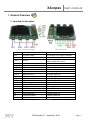
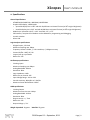
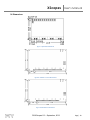
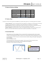
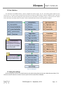
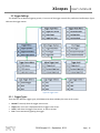
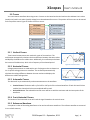
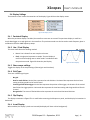
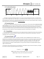
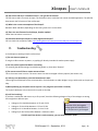
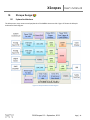
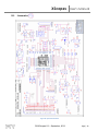
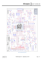
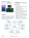
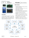
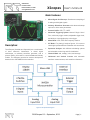
Gabotronics PO BOX 110332 Lakewood Rch, FL. 34211 www.gabotronics.com XScopes User’s Manual Main Features: Mixed Signal Oscilloscope: Simultaneous sampling of 2 analog and 8 digital signals. Arbitrary Waveform Generator with advanced sweep options on all the wave parameters. Protocol Sniffer: SPI, I C, UART Advanced Triggering System: Normal / Single / Auto / 2 Free, with many trigger modes; adjustable trigger level, and ability to view signals prior to the trigger. Figure 1: Xprotolab and Xminilab, Top View Meter Mode: VDC, VPP and Frequency readout. XY Mode: For plotting Lissajous figures, V/I curves or Description: checking the phase difference between two waveforms. The XScopes (Xminilab and Xprotolab) are a combination of three electronic instruments: a mixed signal oscilloscope, an arbitrary waveform generator, and a protocol sniffer; all housed in a small breadboard friendly module. The XScopes can also be used as development boards for the AVR XMEGA microcontroller. Spectrum Analyzer with different windowing options and selectable vertical log and IQ visualization. Channel Math: add, multiply, invert, and average. Horizontal and Vertical Cursors with automatic waveform measurements, and waveform references. Figure 2: XScopes Block Diagram DS-XScopes-2.2 – September, 2012 Page | 1 XScopes User’s Manual About this manual This manual targets both novice and advanced users, providing a full resource for everyone. However, for a full understanding of the operation of the XScopes, the user should be familiar with the operation of a regular oscilloscope. The features documented in this manual are for the Xminilab hardware version 2.1+ or Xprotolab hardware version 1.7+, with firmware version 2.00+. Conventions XScope: Xprotolab or Xminilab CH1: Analog Channel 1 CH2: Analog Channel 2 CHD: Logic Inputs Fast Sampling: 10ms/div or faster Slow Sampling: 20ms/div or slower Helpful tip Technical Detail Revision History Version 1.0 1.1 1.2 1.3 1.5 1.6 1.7 1.8 1.9 2.0 2.1 2.2 Date September 2011 December 2011 January 2012 January 2012 January 2012 February 2012 March 2012 June 2012 August 2012 August 2012 September 2012 September 2012 Notes First revision Firmware upgrade for HW 1.7 Updated AWG maximum frequency to 125kHz Added vertical sensitivity on specifications Changed seconds units from S to s Corrected discrepancies in the interface protocol Added maximum screen refresh rate Merged Xprotolab and Xminilab manual, added new features Documented latest features Added a chapter with examples Documented the Frequency Counter Updated Frequency Counter DS-XScopes-2.2 – September, 2012 Page | 2 XScopes User’s Manual TABLE OF CONTENTS 1. General Overview.......................................................................................................................... 7 1.1 Xprotolab Pin Description ............................................................................................................ 7 1.2 Xminilab Pin Description .............................................................................................................. 8 1.3 Specifications ................................................................................................................................ 9 1.4 Dimensions ................................................................................................................................... 10 1.5 Absolute Maximum Ratings ...................................................................................................... 11 1.6 Factory Setup .............................................................................................................................. 11 1.7 Quick Start Guide ....................................................................................................................... 11 1.8 User Interface .............................................................................................................................. 12 1.9 Saving the settings ...................................................................................................................... 12 2. Mixed Signal Oscilloscope ......................................................................................................... 13 2.1 Horizontal Settings....................................................................................................................... 13 2.1.1 Time Base................................................................................................................................... 13 2.1.2 Technical Details ...................................................................................................................... 13 2.1.3 Horizontal Position .................................................................................................................... 13 2.1.4 Auto Setup ................................................................................................................................ 13 2.2 Vertical Settings .......................................................................................................................... 14 2.2.1 Disable Channel ....................................................................................................................... 14 2.2.2 Channel Gain ........................................................................................................................... 14 2.2.3 Channel Position....................................................................................................................... 14 2.2.4 Channel Invert .......................................................................................................................... 14 2.2.5 Channel Math........................................................................................................................... 14 2.3 Trigger Settings ............................................................................................................................ 15 2.3.1 Trigger Types.............................................................................................................................. 15 2.3.2 Trigger Modes ........................................................................................................................... 16 2.3.3 Trigger Hold ............................................................................................................................... 17 2.3.4 Post Trigger ................................................................................................................................ 17 DS-XScopes-2.2 – September, 2012 Page | 3 XScopes 2.3.5 User’s Manual Trigger Source ........................................................................................................................... 17 2.4 Device Modes ............................................................................................................................. 18 2.4.1 Oscilloscope Mode .................................................................................................................. 18 2.4.1.1 Roll Mode .................................................................................................................................. 18 2.4.1.2 Elastic Traces ............................................................................................................................ 18 2.4.1.3 XY Mode.................................................................................................................................... 19 2.4.2 Meter Mode .............................................................................................................................. 19 2.4.2.1 Frequency Measurements...................................................................................................... 19 2.4.3 Spectrum Analyzer ................................................................................................................... 20 2.4.3.1 IQ FFT Mode .............................................................................................................................. 20 2.4.3.2 Logarithm display .................................................................................................................... 20 2.4.3.3 FFT Windows .............................................................................................................................. 20 2.5 Cursors .......................................................................................................................................... 21 2.5.1 Vertical Cursors ......................................................................................................................... 21 2.5.2 Horizontal Cursors ..................................................................................................................... 21 2.5.3 Automatic Cursors .................................................................................................................... 21 2.5.4 Track Horizontal Cursors ........................................................................................................... 21 2.5.5 Reference Waveform .............................................................................................................. 21 2.6 Display Settings ........................................................................................................................... 22 3. 2.6.1 Persistent Display ...................................................................................................................... 22 2.6.2 Line / Pixel Display .................................................................................................................... 22 2.6.3 Show scope settings ................................................................................................................ 22 2.6.4 Grid Type ................................................................................................................................... 22 2.6.5 Flip Display ................................................................................................................................. 22 2.6.6 Invert Display ............................................................................................................................. 22 Logic Analyzer and Protocol Sniffer ........................................................................................... 23 DS-XScopes-2.2 – September, 2012 Page | 4 XScopes User’s Manual 3.1 Input Selection ............................................................................................................................ 23 3.2 Channel Position ......................................................................................................................... 23 3.3 Invert Channel ............................................................................................................................ 23 3.4 Thick Logic ‘0’.............................................................................................................................. 23 3.5 Parallel Decoding ....................................................................................................................... 24 3.6 Serial Decoding .......................................................................................................................... 24 3.7 Protocol Sniffer ............................................................................................................................ 24 3.8 Sniffers Modes ............................................................................................................................. 24 3.9 I2C Sniffer ..................................................................................................................................... 25 4. 3.10 UART Sniffer ........................................................................................................................... 25 3.11 SPI Sniffer ............................................................................................................................... 25 Arbitrary Waveform Generator ................................................................................................... 26 4.1 Predefined Waveforms .............................................................................................................. 27 4.2 Parameter Sweep....................................................................................................................... 27 4.2.1 Sweep Modes ........................................................................................................................... 27 4.3 Technical Details......................................................................................................................... 27 5. PC Interface .................................................................................................................................. 28 6. Interface Protocol ........................................................................................................................ 28 6.1 Interface settings ........................................................................................................................ 28 6.2 Control data ................................................................................................................................ 28 6.2.1 Bitfield variables ........................................................................................................................ 30 6.3 Command Set............................................................................................................................. 31 6.4 Vendor ID and Product ID ......................................................................................................... 32 7. BMP Screen Capture .................................................................................................................... 33 7.1 To send a BMP screen capture to a PC: ................................................................................. 33 7.2 To send a BMP screen capture to Linux: ................................................................................. 34 8. XScope’s Examples ..................................................................................................................... 35 DS-XScopes-2.2 – September, 2012 Page | 5 XScopes User’s Manual 8.1 Resistor Voltage Divider ............................................................................................................. 35 8.2 Measurement of an RC time constant ................................................................................... 35 8.3 Half Wave Rectifier with Smoothing Capacitor ..................................................................... 35 8.4 BJT Amplifier ................................................................................................................................. 36 8.5 Component V/I Curves ............................................................................................................. 36 8.6 Frequency Plots ........................................................................................................................... 36 9. Firmware Updating....................................................................................................................... 37 9.1 Firmware upgrade using an external programmer .............................................................. 37 9.1.1 Tools required ............................................................................................................................ 37 9.1.2 Instructions to install the tools ................................................................................................. 37 9.1.3 Instructions to update the firmware ...................................................................................... 37 9.2 Firmware upgrade using the bootloader ............................................................................... 38 9.2.1 Tools required ............................................................................................................................ 38 9.2.2 Activating the bootloader ...................................................................................................... 38 9.2.1 FLIP application instructions .................................................................................................... 38 10. Frequently Asked Questions ....................................................................................................... 39 11. Troubleshooting ............................................................................................................................ 40 12. XScope Design ............................................................................................................................. 41 12.1 System Architecture ............................................................................................................ 41 12.2 Schematics ........................................................................................................................... 42 DS-XScopes-2.2 – September, 2012 Page | 6 XScopes User’s Manual 1. General Overview 1.1 Xprotolab Pin Description K1 K2 K3 K4 Figure 4: Front and Top Signals Figure 3: Back Signals Name +5V -5V Description +5V Input voltage -5V Output voltage GND Ground +3.3V Logic 0 Logic 1 Logic 2 Logic 3 Logic 4 Logic 5 Logic 6 Logic 7 EXT. T AWG CH2 CH1 PWR RX TX LNK +3.3V Output voltage Digital Channel 0 Digital Channel 1 Digital Channel 2 Digital Channel 3 Digital Channel 4 Digital Channel 5 Digital Channel 6 Digital Channel 7 External Trigger Arbitrary Waveform Generator Analog Channel 2 Analog Channel 1 Power up output signal Interface RX input Interface TX output Interface link input Comment Do not apply +5V if using the USB port 50mA max output It is recommended use all ground pins to reduce voltage offset errors. 200mA max output I2C Sniffer signal: SDA I2C Sniffer signal: SCL UART Sniffer signal: RX UART Sniffer signal: TX SPI Sniffer signal: /SS SPI Sniffer signal: MOSI SPI Sniffer signal: MISO SPI Sniffer signal: SCK Digital input, max 5.5V Output range: +/- 2V Input range: -14V to +20V Input range: -14V to +20V 3.3V signal, 10mA max output Connect to host’s TX Connect to host’s RX 3.3V level input, with internal pull up Table 1: Pin description DS-XScopes-2.2 – September, 2012 Page | 7 XScopes User’s Manual 1.2 Xminilab Pin Description Figure 5: Xminilab HW 2.1 & 2.2 Front Signals K1 K2 K3 K4 Figure 6: Xminilab HW 2.3 Front Signals K1 Name CH1 CH2 AWG EXT. T Logic 0 Logic 1 Logic 2 Logic 3 Logic 4 Logic 5 Logic 6 Logic 7 +3.3V +5V GND PWR RX TX LNK K2 Description Analog Channel 1 Analog Channel 2 Arbitrary Waveform Generator External Trigger Digital Channel 0 Digital Channel 1 Digital Channel 2 Digital Channel 3 Digital Channel 4 Digital Channel 5 Digital Channel 6 Digital Channel 7 +3.3V Output voltage +5V Input voltage Ground Power up output signal Interface RX input Interface TX output Interface link input K3 K4 Comment Input range: -14V to +20V Input range: -14V to +20V Output range: +/- 2V Digital input, max 5.5V I2C Sniffer signal: SDA I2C Sniffer signal: SCL UART Sniffer signal: RX UART Sniffer signal: TX SPI Sniffer signal: /SS SPI Sniffer signal: MOSI SPI Sniffer signal: MISO SPI Sniffer signal: SCK 200mA max output Do not apply +5V if using the USB port It is recommended use all ground pins 3.3V signal, 10mA max output Connect to host’s TX Connect to host’s RX 3.3V level input, with internal pull up Table 2: Xminilab Pin Description DS-XScopes-2.2 – September, 2012 Page | 8 XScopes 1.3 User’s Manual Specifications General Specifications: - - ATXMEGA32A4 36KB Flash, 4KB SRAM, 1KB EEPROM. Graphic OLED display, 128x64 pixels. o Xprotolab display size is 0.96” and with 10,000 hours minimum life time (to 50% original brightness). o Xminilab display size is 2.42” and with 40,000 hours minimum life time (to 50% original brightness). Module size: Xprotolab: 1.615" x 1.01". Xminilab: 3.3” x 1.75” PDI interface, an optional 2x3 headers can be soldered for programming and debugging. 4 tactile switches. Micro USB. Logic Analyzer specifications: - 8 Digital Inputs, 3.3V level Maximum sampling rate: 2Msps Frequency Counter: 12MHz, +/- 1Hz resolution, +/-100ppm accuracy Protocol Sniffer: UART, I2C, SPI Internal pull up or pull down Buffer size: 256 Oscilloscope specifications: - 2 Analog Inputs Maximum Sampling rate: 2Msps Analog Bandwidth: 200kHz Resolution: 8bits Input Impedance: 1MΩ Buffer size per channel: 256 Input Voltage Range: -14V to +20V Vertical sensitivity: 80mV/div to 5.12V/div Maximum Screen Refresh Rate: 128Hz AWG specifications: - 1 Analog Output Maximum conversion rate: 1Msps Analog Bandwidth: 44.1kHz Resolution: 8bits Output current > +/- 7mA Buffer size: 256 Output Voltage: +/- 2V Weight: Xprotolab: 10 grams. Xminilab: 25 grams. DS-XScopes-2.2 – September, 2012 Page | 9 XScopes User’s Manual 1.4 Dimensions Figure 7: Xprotolab Dimensions Figure 8: Xminilab 2.1 & 2.2 Dimensions Figure 9: Xminilab 2.3 Dimensions DS-XScopes-2.2 – September, 2012 Page | 10 XScopes User’s Manual 1.5 Absolute Maximum Ratings Parameter Supply Voltage (+5V) Analog Inputs Digital Inputs External Trigger Operating Temperature Storage Temperature Minimum -0.5 -30 -0.5 -2.2 -40 -40 Maximum 5.5 30 3.8 5.5 70 80 Unit V V V V °C °C Table 3: Absolute Maximum Ratings 1.6 Factory Setup The device can enter factory options if the MENU key is pressed during power up. The following options are available: 1) Offset calibration: The unit is calibrated before being shipped, but calibration is required again if the firmware is updated. During calibration, two graphs are shown that represent the calibration on each channel. 2) Sleep timeout: Sets the time to shut down the display and put the microcontroller to sleep after the last key press. Shutting down the OLED extends its life. The current consumption.is also reduced. 3) Restore defaults: Select this function to restore to the default the settings. There are many settings on the device, if you are not familiar with them, this function is useful to set the device to a known state. 1.7 Quick Start Guide - - Take the device out of the packaging. There is a protective film on the display which can be removed. The device can be powered with either the USB or with an external power supply, by applying +5V on the corresponding pin. Double check your connections because the device WILL get damaged if applying power on the wrong pin. Connect the AWG pin to CH1. The tactile switches are named (from left to right) K1, K2, K3 and K4. The K4 is the Menu button. Press and hold the K1 key (auto setup). The screen should look like figure 10. Pressing K2 or K3 will change the sampling rate. Additional examples on how to use the Xprotolab are presented in chapter 8. Figure 10: Quick start DS-XScopes-2.2 – September, 2012 Page | 11 XScopes User’s Manual 1.8 User Interface The K4 button is the MENU button, used to navigate thru all the menus. The K1 - K3 buttons action depend on the current menu. The green arrows represent the flow when pressing the MENU button. When the MENU button is pressed on the last menu, the device settings are saved and the menu goes back to the default. Figure 11 shows the main menus in blue and some secondary menus in yellow. Further ramifications are shown on the respective chapters. If confused while navigating the menus, it is easy to go back to the default menu by pressing the MENU button a few times. A green arrow represents the flow when pressing the MENU button Figure 11: Main Menus 1.9 Saving the settings All the settings are stored to non-volatile memory only when exiting from the last menu (Miscellaneous Menu). This method is used to reduce the number of write cycles to the microcontroller’s EEPROM. DS-XScopes-2.2 – September, 2012 Page | 12 XScopes User’s Manual 2. Mixed Signal Oscilloscope The XScope is a mixed signal oscilloscope; it has 2 analog channels and 8 digital channels. This chapter will focus on the analog signals. More information about the digital channels is presented in chapter 3. 2.1 Horizontal Settings The horizontal settings are controlled on the default menu. The menu is shown on figure 12. 2.1.1 Time Base The time base can be varied from 8µs/div to 50s/div. Table 4 shows all the possible time bases. One time division consists of 16 pixels. Example: 8µs / division = 8µs / 16 pixels 500ns / pixel. Time Base ( s / div ) Fast Slow *8µ 20m 16µ 50m 32µ 0.1 64µ 0.2 128µ 0.5 256µ 1 Figure 12: Horizontal Menus 500µ 2 1m 5 2m 10 5m 20 10m 50 Table 4: Time divisions *At 8µs/div, CH2 is not displayed. 2.1.2 Technical Details There are two distinct sampling methods: Fast Sampling and Slow Sampling. - Fast Sampling (10ms/div or faster): All samples are acquired to fill the buffer, and then they are displayed on the screen. o Pre-trigger sampling (ability to show samples before the trigger) is available only with fast sampling. o Only 128 samples are visible at a time, varying the horizontal position allows exploring the full buffer. - Slow Sampling (20ms/div or slower): Single samples are acquired and simultaneously displayed on the display. o The ROLL mode (waveform scrolls to the left during acquisition) is only available with the slow sampling. o All 256 samples are visible on the display (each vertical line will have at least two samples) 2.1.3 Horizontal Position The horizontal position can be varied on the Fast Sampling time bases. There are 256 samples for each channel, but only 128 are displayed on the screen. When the acquisition is stopped, the full sample buffer can be explored with the K2 and K3 buttons. Pressing K2 and K3 simultaneously on the default menu will center the horizontal position. 2.1.4 Auto Setup The Auto Setup feature will try to find the optimum gain and time base for the signals being applied on CH1 and CH2. DS-XScopes-2.2 – September, 2012 Page | 13 XScopes User’s Manual 2.2 Vertical Settings The analog channel controls are discussed in this section. Figure 13 shows the Vertical menu flow. CH1 and CH2 have identical settings. Figure 13: Vertical menus 2.2.1 Disable Channel Any channel can be disabled; this is useful to reduce clutter on the display. 2.2.2 Channel Gain Table 5 shows the possible gain settings for the analog channels. One gain division consists of 16 pixels. The current gain settings for the analog channels are shown in the top right part of the display (If the SHOW setting of the display is enabled). 2.2.3 Channel Position Gain Settings (Volts / Division) 5.12 2.56 1.28 0.64 0.32 0.16 80m Table 5: Gain Settings The position of the waveform can be moved up or down in the Channel Position menu. 2.2.4 Channel Invert The channel can be inverted. The displayed waveform and channel calculations will be affected. 2.2.5 Channel Math - 8 16 32 10 20 50 100 200 500 1 2 5 10 20 50 Subtract: The channel trace will be replaced with the difference. Multiply: The channel trace will be replaced with the product. Average: The channel samples will be averaged to reduce aliasing. (See Figure 14). Channel Math Examples: Figure 16: Two signals Figure 15: CH1+CH2 Figure 17: CH1xCH2 To display CH1+CH2, first invert CH2 and then select the SUBTRACT function. µs/div: 1 us/div: 1 µs/div to ms/div: 2 ms/div: 1 ms/div: 2 ms/div: 4 ms/div: 8 ms/div: 20 s/div: 40 s/div: 80 s/div: 200 s/div: 400 s/div: 800 s/div:2000 sample sample (no average) (no average) samples sample samples samples samples samples samples samples samples samples samples samples are (no are are are are are are are are are are averaged average) averaged averaged averaged averaged averaged averaged averaged averaged averaged averaged Figure 14: Number of samples averaged when enabling the channel AVERAGE option. The device’s sampling rate is normally faster than needed to be able to average samples DS-XScopes-2.2 – September, 2012 Page | 14 XScopes User’s Manual 2.3 Trigger Settings The XScope has an advance triggering system, it has most of the trigger controls of a professional oscilloscope. Figure 18 shows the trigger menus. Figure 18: Trigger menus 2.3.1 Trigger Types There are four different trigger types, which determine when to display the trace on the screen: Normal: Trace only when the trigger event occurs. Single: Only one trace is displayed when the trigger event occurs. Auto: Trace when the trigger event occurs, or after a timeout. Free: Trace continuously ignoring the trigger. DS-XScopes-2.2 – September, 2012 Page | 15 XScopes User’s Manual 2.3.2 Trigger Modes Three triggering modes are available: Edge, Window, and Slope. The Edge and Slope have selectable direction. The direction of the trigger is changed in the “Adjust Trigger Level” menu, by moving up or moving down the trigger level. Edge Trigger: The trigger occurs when the signal crosses the trigger level in a certain direction. The trigger level is represented on the display as a rising ( ), falling ( ) or dual arrow ( ). o Rising edge: The trigger occurs when the signal crosses the level from below to above. o Falling Edge: The trigger occurs when the signal crosses the level from above to below. o Dual Edge: The trigger occurs when the signal crosses the trigger level in any direction. To select the Dual Edge mode, deselect Window, Edge, and Slope in the “Trigger Mode Menu”, the trigger mark will change to a dual arrow: Edge Trigger: The signal crosses a level. Figure 19: Edge Trigger Window Trigger: The trigger occurs when the signal leaves a voltage range. This mode is useful for detecting overvoltages or undervoltages. Two arrow trigger marks represent the window levels. Window Trigger: The signal is outside a range. Figure 20: Window Trigger Slope Trigger: The trigger occurs when the difference between two consecutive samples is greater or lower than a predefined value. This is useful for detecting spikes or for detecting high frequency signals. The trigger mark is represented on the screen as two small lines, with a size proportional to the trigger value. Slope Trigger: The difference of two points in the signal is above a value. Figure 21: Slope trigger DS-XScopes-2.2 – September, 2012 Page | 16 XScopes User’s Manual 2.3.3 Trigger Hold The trigger hold specifies a time to wait before detecting the next trigger. It is useful when the signal can have multiple trigger events occurring close to each other, but you only want to trigger on the first one. 2.3.4 Post Trigger The oscilloscope is continuously acquiring samples in a circular buffer. Once the trigger event occurs, the oscilloscope will acquire more samples, specified by the Post Trigger value. The ability to show samples before or after the trigger is one of the most powerful features of a digital sampling oscilloscope. The post trigger is only available on the fast sampling rates. Depending on the post trigger settings, different parts of a signal can be displayed. Consider the signal on figure 22: Figure 22: Sample signal Even though the buffer sample is relatively small, any section of the shown figure can be analyzed by varying the post trigger value. Examples: - Post trigger = 0 (don’t acquire more signals after the trigger). Only the signals that occurred before the trigger event are shown. Figure 23: Post trigger value equal zero - Post trigger = 50% of the sample buffer (default setting). Half of the buffer contains samples before the trigger, and half contains the samples after the trigger. Figure 24: Post trigger = 50% of sample buffer - Post trigger = 100% of the sample buffer Only signals immediately after the trigger event are shown. Figure 25: Post trigger = 100% of buffer The actual post trigger value can vary between 0 and 32768 samples, so you can explore the signal after a very long time after the trigger event has occurred, but with a high post trigger value, the refresh rate of the scope will be reduced. 2.3.5 Trigger Source Any analog or digital channel can be the trigger source. If selecting a digital channel as trigger source, the slope and window modes are not applicable; the device will use edge triggering. The external trigger input is an additional digital trigger source which tolerates voltages up to 5.5V. DS-XScopes-2.2 – September, 2012 Page | 17 XScopes User’s Manual 2.4 Device Modes There are multiple device modes that can be selected; the menus shown on figure 26 allow selecting the Scope Mode, the Meter Mode or the Spectrum Analyzer Mode (FFT). Another device mode is the Protocol Sniffer, which is discussed in section 3.8. In the “Mode Menu”, press K1 and K3 simultaneously, to display both the Scope and FFT. Figure 26: Device mode menus 2.4.1 Oscilloscope Mode This is the default mode of the XScope. The 2 analog and 8 digital channels are sampled simultaneously. Any of these 10 channels can be shown on the display. Figure 27 shows the oscilloscope mode and the various sections of the display are detailed. Green LED: Flashes after every screen refresh Trigger level mark Red LED: Flashes with USB activity Scope Settings: Channel Gain Time Base The scope can also display the traces in XY mode, which is described in section 2.4.1.3 Grid Figure 27: Oscilloscope Mode 2.4.1.1 Roll Mode The data on the display is scrolled to the left as new data comes in. This is only available on the Slow Sampling rates. The Roll mode and Elastic mode cannot be selected simultaneously. The Roll mode disables the triggering. 2.4.1.2 Elastic Traces This is also called “Display average” on other digital oscilloscopes. It works by averaging the trace data with the new data. The result is a more stable waveform displayed on the screen. However, using this setting only makes sense when the scope is properly triggered. The Elastic trace computes this equation for every point in the trace: DS-XScopes-2.2 – September, 2012 Page | 18 XScopes 2.4.1.3 User’s Manual XY Mode The XY mode changes the display from volts vs. time display to volts vs. volts. You can use XY mode to compare frequency and phase relationships between two signals. XY mode can also be used with transducers to display strain versus displacement, flow versus pressure, volts versus current, or voltage versus frequency. Lissajous figures can also be plotted using the XY Mode. Component curves can also be plotted, see section 8.5. When using the XY modes with a Slow Sampling rate, activating the ROLL mode will display a continuous “beam”. Figure 28: XY Mode 2.4.2 Meter Mode The XScope can function as a dual digital voltmeter. The font used is bigger in meter mode to facilitate reading. The available measurements in meter mode are: Average Voltage (DC), Peak to Peak Voltage, and Frequency. A small trace of the analog signals is displayed below the measurements. Figure 29: Meter Mode If there is more than 10mV of voltage in the VDC measurement with no signal, recalibrate the device’s offset (Section 1.6). 2.4.2.1 Frequency Measurements The device can measure frequencies on the analog channels and on the external trigger pin. Frequency measurements on the analog channels are done using the FFT of the acquired data, so measured frequencies have discrete steps. The frequency range is determined by the highest frequency of the analog channels. If there is a high frequency on one channel and a low frequency on the other, the channel with the lowest frequency will have low resolution. Frequency measurements with the FFT are best suited for analog signals. Frequency measurements on the external trigger are done counting the pulses on the pin over one second. The resolution of the measurement is 1Hz. Frequency measurements with the Freq. counter are best suited for digital signals. Maximum voltage range Maximum Frequency Resolution Signal is noisy, or is mixed with other signals Signal has a high offset FFT (Analog channels) -14V to 20V 500kHz Variable, depending on frequency range. From 6.25Hz to 7.812kHz Finds the fundamental frequency Frequency Counter (Ext. Trigger) -2.2V to 5.5V Over 12MHz 1Hz Still works Stops working when the offset is above the logic threshold. Not suitable Table 6: FFT vs. Frequency Counter DS-XScopes-2.2 – September, 2012 Page | 19 XScopes User’s Manual 2.4.3 Spectrum Analyzer The spectrum analyzer is done by calculating the Fast Fourier Transform (FFT) of the selected analog channels (or the channel math functions if enabled). When the FFT is enabled, the spectrum is plotted as frequency vs. magnitude. The horizontal axis represents the frequency (Hertz), and the vertical axis represents the magnitude. Figure 30 shows the XScope in Spectrum Analyzer Mode. The Nyquist frequency is shown on the top right corner of the display. Figure 30: Spectrum Analyzer Mode If only interested in one channel, turn off the other channel to maximize the vertical display. 2.4.3.1 IQ FFT Mode When the IQ FFT is disabled, the XScope calculates two independent 256 point FFTs of the analog channels, the Real and Imaginary components of the FFT have the same data. The output of the FFT is symmetrical, but only half of the result is shown on the display. When the IQ FFT is enabled, only one FFT is calculated, the Real component is filled with the CH1 data, and the Imaginary component is filled with the CH2 data. The result is a 256 point FFT, you can use the horizontal controls described in section 2.1.3 to explore all the data (since only 128 points can be shown on the display). The IQ FFT is useful to monitor RF Spectrums with the proper hardware mixer. 2.4.3.2 Logarithm display The log is useful when analyzing low level components on the signal. When analyzing audio, it is also very useful as it maps more directly to how humans perceive sound. The actual function performed is: y = 16 * log2(x). Example: Figure 33: FFT without Log Figure 31: Triangle Wave 2.4.3.3 Figure 32: FFT with Log FFT Windows To reduce the spectral leakage, an FFT window function can be applied. Four FFT window types are available: Rectangular: No window applied Hamming: Hann: Blackman: ( ( ( ) )) ( ) Figure 34: Window and sine frequency response, from left to right: Rectangular, Hamming, Hann and Blackman DS-XScopes-2.2 – September, 2012 Page | 20 XScopes User’s Manual 2.5 Cursors You can measure waveform data using cursors. Cursors are horizontal and vertical markers that indicate X-axis values (usually time) and Y-axis values (usually voltage) on a selected waveform source. The position of the cursors can be moved on the respective menu. Figure 35 shows the cursor menus. Figure 35: Cursor menus 2.5.1 Vertical Cursors Time interval measurements are made with a pair of time markers. The oscilloscope automatically calculates the time difference between the two markers and displays the difference as a delta time. Additionally, the oscilloscope calculates the inverse of the delta time, which is the frequency of the selected period. Figure 36: Vertical Cursors 2.5.2 Horizontal Cursors Voltage measurements are made with a pair of voltage markers to determine 1 or 2 specific voltage points on a waveform. The oscilloscope automatically calculates the voltage difference between the two markers and displays the difference as a delta voltage value. 2.5.3 Automatic Cursors The device will try to automatically make measurements on the waveform. Figure 37: Horizontal Cursors Vertical Cursors: The device will try find a full or half cycle of the selected waveform. If both CH1 and CH2 are enabled, the channel with the most amplitude will be used. Horizontal Cursor: The selected horizontal cursor will be set with the maximum and minimum points of the waveform. 2.5.4 Track Horizontal Cursors The location of the horizontal cursor will track the signal located on the vertical cursor. 2.5.5 Reference Waveform A snapshot is taken of the analog waveforms to be used as reference waveforms. The reference waveforms are stored in non-volatile memory. DS-XScopes-2.2 – September, 2012 Page | 21 XScopes User’s Manual 2.6 Display Settings These menus control various characteristics of the display. Figure 38 show the display menus. Figure 38: Display menus 2.6.1 Persistent Display When the persistent display is enabled, the waveform traces are not erased. The persistent display is useful as a simple data logger or to catch glitches in the waveform. The persistent mode can also be used to make frequency plots in combination with the AWG frequency sweep. 2.6.2 Line / Pixel Display This menu item selects the drawing method. Line: A line is drawn from one sample to the next. Pixel: A single pixel represents a sample. The pixel display is useful at slow sampling rates or when used in combination with the persistent mode. Figure 39 shows the pixel display. Figure 39: Pixel Display 2.6.3 Show scope settings Toggles the display of the scope settings (Channel gain and time base). 2.6.4 Grid Type There are 4 different grid types: - - No grid. Dots for each division: Vertical dots represent the scale divisions. Horizontal dots represent the time base setting and the ground level of each channel. Vertical grid line follow trigger: Vertical dots represent the position of the trigger, the location of the vertical dots follow the trigger position. Horizontal dots represent the time base setting and the ground level of each channel. Dot graticule: The screen is filled with dots that represent the vertical and horizontal divisions. 2.6.5 Flip Display The display orientation is flipped. This is useful when mounting the XScope on a panel, and the display’s orientations is backwards. 2.6.6 Invert Display When enabled, the display’s pixels are inverted (the display will have a white background). DS-XScopes-2.2 – September, 2012 Page | 22 XScopes User’s Manual 3. Logic Analyzer and Protocol Sniffer The XScope has an 8 bit logic analyzer and can do sniffing on standard protocols: I2C, UART and SPI. The logic inputs are 3.3V level (the logic inputs are not 5V tolerant!). If you need to connect 5V signals to the logic analyzer, you could add a 3K resistor in series with the signal, or use a 5V to 3.3V level converter chip. Figure 40 shows the logic menus. Figure 40: Logic Analyzer Menus 3.1 Input Selection A subset of the 8 digital signals can be selected. Any digital signal can be enabled or disabled. 3.2 Channel Position The selected digital channels can be moved up or down. Only applicable if less than 8 digital signals are selected. 3.3 Invert Channel All digital channels are inverted. This setting also affects the protocol sniffer!. 3.4 Thick Logic ‘0’ A thick line is drawn when the signal is at logic ‘0’. This is useful to quickly differentiate a ‘0’ from a ‘1’. DS-XScopes-2.2 – September, 2012 Page | 23 XScopes User’s Manual 3.5 Parallel Decoding Shows the hexadecimal value of the 8 bit digital input lines. The hexadecimal number is shown below the last digital trace. If all the 8 digital traces are enabled, then there is no space to show the parallel decoding. Figure 41 shows an example of the parallel decoding with 4 logic lines enabled. Figure 41: Parallel Decoding 3.6 Serial Decoding Shows the hexadecimal value of the stream of bits on each channel. The decoding starts at the first vertical cursor and ends at the second vertical cursor, 8 bits are decoded. If the cursors are disabled, then the decoding is done from the start of the screen, to the end. The data can be decoded MSB first or LSB first, depending on the position of the first vertical cursor. Figure 42: Serial Decoding 3.7 Protocol Sniffer When the XScope is in Sniffer mode, a small text appears on the screen before any data is received, to indicate where to hook up the signals. As soon as the data is received, the data is displayed in "pages". There are 16 pages of data. To browse thru the pages, use the buttons K2 and K3. To stop and start the sniffer, press the K1 button. Figure 43 shows the device in sniffer mode. Figure 43: Sniffer In the UART and SPI sniffers, the data can be displayed in HEX or ASCII, press K2 and K3 simultaneously to toggle between them. If using ASCII, only codes 0x20 thru 0x7A will show valid characters. Figure 44 shows the 3x6 font. 3.8 Sniffers Modes Figure 44: Small 3x6 font Normal mode: Continuous operation, when the buffer is filled, all pages are erased, the index goes back to page 1 Single mode: The sniffer will stop when the buffer is filled. Circular mode: New data will be placed at the end of the last page, older data will be shifted towards the first page. At the beginning, the device will show 0x00 an all pages, and the last page will be set. DS-XScopes-2.2 – September, 2012 Page | 24 XScopes User’s Manual 3.9 I2C Sniffer Connect SDA to Bit 0, SCL to Bit 1 The XScope implements the I2C sniffing in a bit-bang fashion. The maximum tested clock frequency is 400kHz (Standard I2C Fast Speed). As the data is decoded, the data in HEX will appear on the screen, accompanied by a symbol: When the Master initiates a read, < is an ACK and ( is a NACK When the Master initiates a write, > is an ACK and ) is a NACK Subsequent data in the frame will be accompanied by + for ACK or a - for NACK. There are 16 pages of data, each page shows 64 bytes => the total memory for the I2C sniffer is 1024 bytes. Example communicating to a Si570 Programmable oscillator: 55> 07+ (Master initiates Write to slave 55, byte address 7) 55< 05+ 42+ B6+ 04+ 79+ 9A- (Master initiates Read to slave 55, then reads 6 bytes) 3.10 UART Sniffer Connect RX to Bit 2, TX to Bit 3 The XScope can decode both the TX and RX lines of the UART at the standard baud rates: 1200, 2400, 4800, 9600, 19200, 38400, 57600, 115200 The screen is split in two, the left side is used for the RX line, and the right side is used for the TX line. Each side can show 40 bytes per page. With 16 pages, a total of 640 bytes can be stored for each decoded line. Figure 45: UART Sniffer screen 3.11 SPI Sniffer Connect the Select to Bit 4, MOSI to Bit 5, MISO to Bit 6, SCK to Bit 7 The XScope can decode both the MOSI and MISO lines of an SPI bus. The SPI's MOSI pin decoding is done in hardware, so it can decode data at high speed, But the SPI's MISO pin decoding is implemented in software using bit-banging, so the maximum clock allowed will be limited. The screen is split in two, the left side is use for the MOSI line, and the right side is used for the MISO line. Each side can show 40 bytes per page. With 16 pages, a total of 640 bytes can be stored for each decoded line. DS-XScopes-2.2 – September, 2012 Page | 25 XScopes User’s Manual 4. Arbitrary Waveform Generator The XScope has an embedded arbitrary waveform generator. The waveform generator output is independent from the data acquisition and is always running in the background. You can adjust all the parameters of the waveform: frequency, amplitude, offset and duty cycle. You can sweep the frequency, amplitude and duty cycle. Figure 46 shows the AWG Menus. Figure 46: AWG Menus When adjusting the parameters, the K1 button serves as a shortcut key, which sets predefined values . When enabling the Sweep, the waveform will be updated only on a screen refresh. For a smooth sweep, set the scope with a high speed sampling, or stop the oscilloscope. DS-XScopes-2.2 – September, 2012 Page | 26 XScopes User’s Manual 4.1 Predefined Waveforms Sine Wave Square Wave Triangle Wave Exponential Periodic Noise Custom Wave * Table 7 The XScope can output the following waveforms: Sine, Square, Triangle and Exponential. There is a “Periodic Noise” option that fills the AWG buffer with random data, it is periodic because the same data is output over and over, but each time the Noise wave is selected, new random data will be generated. There is also a custom waveform which is initially set with an ECG wave, but can be changed with the PC XScope Interface. 4.2 Parameter Sweep The XScope has a SWEEP feature, which increases one or more parameter values automatically on each screen refresh of the oscilloscope. When the sweep is enabled, three dots will appear at the bottom of the screen, representing the start, end, and current sweep value. When doing a Frequency sweep, the frequency range is determined by the current time base. Since the frequency sweep is synchronized with the oscilloscope, displaying perfect frequency plots is easy. To make a frequency plot, set the mode to FFT, and set the display to persistent. See section 8.6 for an example. 4.2.1 Sweep Modes In the Sweep Mode menu, the sweep direction can be changed. Automatic change of the direction is done by enabling the Ping Pong mode. The sweep acceleration increases or decreases the sweep speed, the sweep speed is reset when reaching the start or end of the sweep. 4.3 Technical Details The waveform is stored in a 256 byte long buffer, this buffer is fed to the XMEGA's DAC thru the DMA. Once the waveform is set, the waveform will be generated without any CPU intervention. The maximum conversion rate of the DAC is 1Msps, this limits the maximum output frequency of the AWG as a system. For example, if the AWG is generating a sinewave with 256 points, the maximum frequency is 3906.25Hz. If generating a sinewave with only 32 points, the maximum frequency is 31.25KHz. The AWG amplifier has a low pass filter of 44.1KHz. The predefined AWG Frequency range is: 1Hz thru 125 kHz The resolution of the waveform generator varies depending on the frequency range: the lower the frequency, the higher the resolution. Note that the possible frequencies are discrete: Cycles: Integer number, with these possible values: 1, 2, 4, 8, 16, 32 Period: Integer number, with values between 32 and 65535 DS-XScopes-2.2 – September, 2012 Page | 27 XScopes User’s Manual 5. PC Interface The XScope can communicate to a PC with USB. It can also communicate using the UART on the external port (by using a UART adapter or the Bluetooth module). Figure 47 shows a snapshot of the PC interface. Figure 47: Xprotolab PC interface 6. Interface Protocol The XScope can communicate to external devices thru the USB or the external port. Each interface can access the Xscope’s main settings. Follow the protocols to make your own applications, or to make devices that attach to the XScope. 6.1 Interface settings The settings for communicating with the serial port are shown in Table 8. If using the USB interface, you can use WinUSB or LibUSB libraries. The USB device’s endpoints have a size of 64 bytes. The device uses BULK IN transfers on endpoint 1 for transferring data (CH1, CH2 and CHD, 256 bytes each), BULK OUT transfers on endpoint 1 to write to the AWG RAM buffer, and CONTROL READ transfers on endpoint 0 for changing and reading settings. Data Bits: 8 Baud rate: 115200 Parity: None Stop Bits: One Handshaking: None Table 8: Serial settings 6.2 Control data All the XScope’s settings are stored in 43 bytes, table 9 shows these variables, section 6.2.1 describes the bitfield variables. DS-XScopes-2.2 – September, 2012 Page | 28 XScopes Index 0 1 2 3 4 5 6 7 8 9 10 11 12 13 14 15 16 17 18 19 20 21 22 23 24 25 26 27 28 29 30 31 32 33 34 35 36 37 38 39 40 41 42 Name Srate CH1ctrl CH2ctrl CHDctrl CHDmask Trigger Mcursors Display MFFT Sweep Sniffer MStatus CH1gain CH2gain HPos VcursorA VcursorB Hcursor1A Hcursor1B Hcursor2A Hcursor2B Thold Tpost L Tpost H Tsource Tlevel Window1 Window2 CH1pos CH2pos CHDpos CHDdecode Sweep1 Sweep2 SWSpeed AWGamp AWGtype AWGduty AWGoffset desiredF LLB desiredF LHB desiredF HLB desiredF HHB Data Type Unsigned 8bit Bit Field 8bit Bit Field 8bit Bit Field 8bit Bit Field 8bit Bit Field 8bit Bit Field 8bit Bit Field 8bit Bit Field 8bit Bit Field 8bit Bit Field 8bit Bit Field 8bit Unsigned 8bit Unsigned 8bit Unsigned 8bit Unsigned 8bit Unsigned 8bit Unsigned 8bit Unsigned 8bit Unsigned 8bit Unsigned 8bit Unsigned 8bit Description Sampling Rate Channel 1 controls Channel 2 controls Logic Analyzer Options 1 Logic enabled bits Trigger control Cursor Options Display Options FFT Options AWG Sweep Options Sniffer Controls Scope Status Channel 1 gain Channel 2 gain Horizontal Position Vertical Cursor A Vertical Cursor B CH1 Horizontal Cursor A CH1 Horizontal Cursor B CH2 Horizontal Cursor A CH2 Horizontal Cursor B Trigger Hold Unsigned 16bit Post Trigger Unsigned 8bit Unsigned 8bit Unsigned 8bit Unsigned 8bit Signed 8bit Signed 8bit Unsigned 8bit Unsigned 8bit Unsigned 8bit Unsigned 8bit Unsigned 8bit Signed 8bit Unsigned 8bit Unsigned 8bit Signed 8bit Trigger Source Trigger Level Windows Trigger Level 1 Windows Trigger Level 2 Channel 1 Position Channel 2 Position Logic Analyzer position Selected Protocol Sweep Start Sweep End Sweep Speed AWG Amplitude AWG Wave Type AWG Duty Cycle AWG Offset Unsigned 32bit AWG Desired Frequency multiplied by 100 User’s Manual Notes Range: [0, 21] 8 us/div to 50 s/div Selects which logic channels are displayed Range: [0,6] 5.12V/div to 80mV/div Range: [0,6] 5.12V/div to 80mV/div Range: [0,127] pixels Range: [0,127] pixels Range: [0,127] pixels Range: [0,127] pixels Range: [0,127] pixels Range: [0,127] pixels Range: [0,127] pixels Range: [0,255] 0 to 255 milliseconds Range: [0, 32767] Indicates how many samples to acquire after the trigger. Default is 128. 0: CH1; 1: CH2; 2-9: CHD; 10: EXT Range: [3,252] Range: [0,255] Range: [0,255] Range: [-128,0] pixels Range: [-128,0] pixels Range: [0,7] 0: SPI; 1: I2C; 2: RS232 Range: [0,255] Range: [0,255] Range: [0,127] Range: [-128,0] 4V to 0V 0: Noise; 1: Sine; 2: Square; 3: Triangle; 4: Custom Range: [1,255] 0.391% to 99.61% Range: [-128,127] +2V to -1.985V Range: [100, 12500000] 1Hz to 125kHz Table 9: Xscope’s settings DS-XScopes-2.2 – September, 2012 Page | 29 XScopes User’s Manual 6.2.1 Bitfield variables Name CH1ctrl and CH2ctrl CHDctrl Trigger Mcursors Display Bits Bit 0: Channel on Bit 1: x10 probe Bit 2: Bandwidth limit Bit 3: AC/DC select Bit 4: Invert channel Bit 5: Average samples Bit 6: Math Active Bit 7: Math operation Bit 0: Channel on Bit 1: Pull Bit 2: Pull Up Bit 3: Low Bit 4: Invert channel Bit 5: Serial Decode Bit 6: Parallel Decode Bit 7: ASCII Sniffer display Bit 0: Normal Trigger Bit 1: Single Trigger Bit 2: Auto Trigger Bit 3: Trigger Direction Bit 4: Round Sniffer Bit 5: Slope Trigger Bit 6: Window Trigger Bit 7: Edge Trigger Bit 0: Roll Scope Bit 1: Automatic Cursors Bit 2: Track Cursors Bit 3: CH1 Horizontal Cursors on Bit 4: CH2 Horizontal Cursors on Bit 5: Vertical Cursor on Bit 6: Reference waveform on Bit 7: Single Sniffer Capture Bit 0: Grid 0 Bit 1: Grid 1 Bit 2: Elastic Display Bit 3: Invert Display Bit 4: Flip Display Bit 5: Persistent Display Bit 6: Line / Pixel Display Bit 7: Show Settings Notes For future hardware For future hardware For future hardware Enables math (addition or multiplication) Subtract (1) or Multiply (0) Pull resistor enabled Pull up (1) or pull down (0) Thick line when logic '0' The Normal Trigger bit must also be enabled for Single Trigger Dual Edge Trigger is enabled by clearing bits 5,6,7. CH1 and CH2 Horizontal cursors are mutually exclusive CH1 and CH2 Horizontal cursors are mutually exclusive 00: No Grid, 01: Dots per division 10: Follow trigger, 11: Graticule Line (1), Pixels (0) DS-XScopes-2.2 – September, 2012 Page | 30 XScopes Name MFFT Sweep Sniffer MStatus Bits Bit 0: Hamming Window Bit 1: Hann Window Bit 2: Blackman Window Bit 3: Vertical Log Bit 4: IQ FFT Bit 5: Scope Mode Bit 6: XY Mode Bit 7: FFT Mode Bit 0: Acceleration Direction Bit 1: Accelerate Sweep Bit 2: Sweep Direction Bit 3: Ping Pong Mode Bit 4: Sweep Frequency Bit 5: Sweep Amplitude Bit 6: Sweep Offset Bit 7: Sweep Duty Cycle Bit 0: Baud 0 Bit 1: Baud 1 Bit 2: Baud 2 Bit 3: CPOL Clock Polarity Bit 4: CPOH Clock Phase Bit 5: Parity Mode Bit 6: Parity Bit 7: Stop Bit Bit 0: Update Bit 1: Update AWG Bit 2: Update MSO Bit 3: Go Sniffer Bit 4: Stop Bit 5: Triggered Bit 6: Meter VDC Bit 7: Meter VPP User’s Manual Notes Only one window must be selected, or none for No Window. Multiple modes can be selected simultaneously. If no bits are set, the Meter mode is displayed. UART Sniffer Baud Rates: 000: 1200 , 001: 2400, 010: 4800, 011: 9600, 100: 19200, 101: 38400, 110: 57600, 111: 115200 Enables parity check Parity Odd (1), Parity Even (0) 1 Stop bit (0), 2 Stop bits (1) Exits triggering if the bit is set The AWG parameters must be updated if the bit is set The MSO parameters must be updated if the bit is set Enters the Sniffer mode if the bit is set Oscilloscope Stopped Oscilloscope Triggered If the bits are cleared, the Meter mode measures frequency Table 10: Bitfield variable description 6.3 Command Set When using the serial port, the commands are sent to the XScope in ASCII format, further data sent or received is in binary. When using the USB interface, the commands are sent as CONTROL READ requests, where the request byte is the command, and the Index and Value are additional parameters sent to the XScope. If the PC is requesting data, it will be returned in the endpoint 0 IN buffer. Table 11 shows the XScope Interface Protocol Command Set. DS-XScopes-2.2 – September, 2012 Page | 31 XScopes Command Description User’s Manual Device Response / Notes The device returns 4 bytes containing the version number in ASCII. a Request firmware version b Writes a byte to the XScope’s Settings, at the specified index. If the Index is below 14, the updatemso bit is automatically set If the Index is above 34, the updateawg is automatically set. When using the USB interface, the Index contains the index, and the Value contains the data. When using the using the Serial interface, two additional bytes must be sent containing the index and data. c Sets the desired AWG Frequency (32bits). When using the USB interface, the Index contains the lower 16bits, the Value contains the high 16bits. When using the Serial interface, 4 additional bytes must be sent (little endian format). d e f g h i Save XScope’s Settings in EEPROM Save AWG wave stored in RAM to EEPROM Stop Scope Start Scope Force Trigger Auto Setup j Sets the desired Post Trigger Value (16bits) p Disable Auto send (Serial interface only) q Enable Auto send (Serial interface only) r s t u w x Request CH1 (Serial interface only) Request CH2 (Serial interface only) Request CHD (Serial interface only) Request settings Request EE waveform (Serial interface only) Send waveform data (Serial interface only) C Request BMP (Serial interface only) When using the USB interface, the Value contains the 16bits. When using the Serial interface, 2 additional bytes must be sent (little endian format). When the Auto send is active, the device will continuously send data, this is to maximize the refresh rate on the PC side. When using fast sampling rates, the device will first fill its buffers, and then send the buffers in bursts. When using slow sampling rates, the PC app will need to keep track of time, as the samples will arrive with no time reference. CH1 data (256 bytes) CH2 data (256 bytes) CHD data (256 bytes) All the settings (43 bytes) are sent to the PC. EE Wave data (256 bytes) 'G' character, which signals the PC that the device is ready, Then the PC sends the data (256 bytes) Then the device sends a 'T' character, which signals the PC that the data was received. 128x64 Monochrome BMP using the XModem protocol Table 11: XScope Command Set 6.4 Vendor ID and Product ID If you are using LibUSB to interface with the device, you will need the VID and PID of the device: VID=16D0 PID=06F9 If you are using WinUSB, you will need the GUID defined on the driver’s .inf file: GUID= 36FC9E60-C465-11CF-8056-444553540000 DS-XScopes-2.2 – September, 2012 Page | 32 XScopes User’s Manual 7. BMP Screen Capture 7.1 To send a BMP screen capture to a PC: You can send a screen capture of the XScope to your PC using HyperTerminal. All the screen captures bitmaps in this manual where generated using this method. The screen capture is done thru the XScope’s serial port. Open HyperTerminal. Enter a name for a new connection (example: scope). Enter the COM port where the device is connected. Select 115200 bits per second, 8 data bits, Parity None, 1 Stop bit, Flow control None. (See figure 48) Figure 48: HyperTerminal Settings In the Transfer menu, select Receive File. Enter a folder where to save the file and use the XMODEM protocol. (See figure 49) DS-XScopes-2.2 – September, 2012 Page | 33 XScopes User’s Manual Figure 49: Receive File Settings Enter a file name with a BMP extension and press OK 7.2 To send a BMP screen capture to Linux: Create the following script and save as capture.sh: capture.sh echo "Please enter filename. e.g capture.bmp" read name stty -F $1 115200 rx -c $name < $1 > $1 To use, make the script executable with “chmod +x capture.sh”. Then enter “./capture.sh” into a terminal followed by the serial device for example “./capture.sh /dev/ttyUSB0”. Then enter a name for the bmp image including the .bmp file extension. Figure 50: Screen capture in Linux DS-XScopes-2.2 – September, 2012 Page | 34 XScopes User’s Manual 8. XScope’s Examples 8.1 Resistor Voltage Divider 1) Build the circuit shown on figure 51. 2) Set the device to Meter mode 3) You should see similar voltages as shown on figure 52. Figure 51: Resistor divider Figure 52: Meter mode Theory of operation: The circuit is a voltage divider, where Vin is 5V, and Vout is the voltage at CH2: 8.2 Measurement of an RC time constant 1) 2) 3) 4) 5) 6) 7) 8) 9) 10) 11) 12) Build the circuit shown on figure 54. Set the time base to 500µs/div. Set the AWG to Square wave, 500Hz, 4V. Set the gain on both channels to 2.56V/div. Figure 53: RC Measurements The display should look similar to figure 53. Figure 54: RC Circuit Now set the time base to 16µs/div. Turn off CH1, set the CH2 gain to 1.28V/div. Adjust the horizontal and CH2 positions so that the rising wave takes most of the screen. Turn on the vertical and CH2 horizontal cursors. Figure 56: Half-life measurement Figure 55: RC Equations Enable the cursors TRACK option. Set the first vertical cursor at the corner of the wave, and the second cursor where the voltage equals 0V. The display should look like figure 55. The measured time, , is the “half-life” time, so Theory of operation: Circuit theory shows that if the RC circuit is fed with a step input, the output will approach a DC value exponentially; figure 55 shows the equation from which we can obtain RC when the half-life value is known. 8.3 Half Wave Rectifier with Smoothing Capacitor 1) 2) 3) 4) 5) 6) Build the circuit shown on figure 58. Set the time base to 2mS/div. Set the AWG to Sine wave, 125Hz, 4V. Set the gain on both channels to 1.28V/div. The display should look like figure 57. If the capacitor is removed, the display should look like figure 59. Figure 57: Half wave rectifier Figure 58: Half wave rectifier circuit Figure 59: Removing the capacitor Theory of operation: The diode will allow current to flow only during the positive half of the sine wave. The output voltage is a little bit lower because of the voltage drop of the diode. When the AWG voltage is negative, the diode acts like an open circuit and the capacitor discharges thru the resistor at an exponential rate. DS-XScopes-2.2 – September, 2012 Page | 35 XScopes User’s Manual 8.4 BJT Amplifier 1) Build the circuit shown on figure 61. 2) Set the time base to 2ms/div 3) Move the position on both channels all the way down (GND reference grid is at the bottom of the screen). Figure 60: BJT Measurements Figure 61: Amplifier circuit 4) Set CH1 to 0.32V/div, Set CH2 to 1.28V/div. 5) Set the AWG to Sine wave, 125Hz, 0.250V amplitude. 6) Increase the AWG offset until the CH2 wave is centered on the display. The display should look like figure 60. Theory of operation: The transistor needs to be biased in its forward active region; this is what the offset in the AWG is for. The output voltage will vary according to the BJT transfer curve: changes in the input make large changes in the output. 8.5 Component V/I Curves 1) 2) 3) 4) 5) 6) Build the circuit shown in figure 64. Set the time base to 500µs/div. Set the AWG to Sine wave, 125Hz, 4V. Set the gain on both channels to 0.64V/div . Enter the CH2 options and select SUBTRACT. Set the device oscilloscope in XY mode. Figure 62: 1N4148 curve Figure 64: Component tester Figure 63: 100nF Capacitor curve Theory of operation: The goal is to plot the component’s voltage, versus the component’s current. Using the integrated waveform generator and an external resistor, we can inject current into the component. The voltage is measured directly using CH1. The current thru the component is the same as the current thru the resistor, the voltage on the resistor is proportional to the current. The voltage on the resistor is equal to CH2-CH1. 1V on the scope will represent 1mA on the component. Figure 62 and figure 63 show examples of V/I curves on components. 8.6 Frequency Plots The AWG sweep function can be used to plot the frequency response of a circuit. This method is not directly a BODE plot since the horizontal axis is not logarithmic, it is linear. 1) Connect the AWG to the input and CH1 to the output. 2) Set the device to FFT mode. 3) Change to the desired time base. The maximum frequency is shown on the top right of the display. 4) Set the AWG to Sine Wave. 5) Enable the Frequency Sweep. 6) Set the AWG Sweep range to 1:255 7) Set the display to persistent. Figure 65 shows an RLC circuit, and figure 66 shows the frequency response. This example shows the vertical scale with the LOG disabled. DS-XScopes-2.2 – September, 2012 Figure 65: RLC Circuit Figure 66: Frequency plot Page | 36 XScopes User’s Manual 9. Firmware Updating This guide will show how to upgrade the firmware on your AVR XMEGA based device. There are two upgrade methods; you can use either one depending on your needs. 9.1 Firmware upgrade using an external programmer 9.1.1 Tools required AVRISP mkII, or similar PDI capable programmer AVR Studio 4 or Atmel Studio 6 IDE (Integrated Development Environment) HEX and EEP files for the device, found on the product's page (Look for the HEX icon). A regular AVR programmer might not work, the programmer needs to be PDI capable. PDI is the new interface to program XMEGA microcontrollers. 9.1.2 Instructions to install the tools Install AVR Studio and USB driver Connect the programmer to the computer and auto install the hardware A more detailed guide on how to install the tools is found here: http://www.atmel.com/dyn/resources/prod_documents/AVRISPmkII_UG.pdf 9.1.3 Instructions to update the firmware 1. Start AVR Studio 2. Connect the cable from the AVRISP to the PDI connector on the board 3. Power the board 4. Press the "Display the 'Connect' dialog" button: . Alternatively, you can go to this menu: Tools-> Program AVR > Connect 5. Select your programmer and port. (AVRISP mkII and AUTO or USB) 6. In the MAIN tab, select the device: ATXMEGA32A4 7. In the programming mode, select PDI 8. To check that everything is ok, press the "Read Signature" button. You will see a message saying that the device matches the signature. 9. Go to the PROGRAM tab 10. In the Flash section, look for the .HEX file and click Program 11. In the EEPROM section, look for the .EEP file and click Program 12. Go to the FUSES tab 13. Set BODPD to BOD enabled in sampled mode 14. Set BODACT to BOD enabled in sampled mode 15. Set BODLVL to 2.9V 16. Click Program 17. After updating the firmware, make sure to recalibrate the device (See section 1.6). DS-XScopes-2.2 – September, 2012 Page | 37 XScopes User’s Manual 9.2 Firmware upgrade using the bootloader 9.2.1 Tools required Standard USB type A to micro USB cable Atmel’s FLIP software: http://www.atmel.com/tools/FLIP.aspx Flip Manual with driver installation procedure: http://www.atmel.com/Images/doc8429.pdf HEX and EEP files for the device, found on the product's page (Look for the HEX icon). 9.2.2 Activating the bootloader The K1 button needs to be pressed while connecting the device to the computer with the USB cable. Once the XScope enters the bootloader, the red LED will be lit, and will blink with USB activity. The XScope will appear as a new device on the host computer, the drivers required are found in the FLIP application folder. 9.2.1 FLIP application instructions 1) 2) 3) 4) 5) Start Flip. Select ATXMEGA32A4U in the device selection list. Select USB as communication medium Open the USB port to connect to the target Make sure the FLASH buffer is selected and check ERASE, BLANK CHECK, PROGRAM, VERIFY. 6) 7) 8) 9) 10) 11) 12) 13) Load the HEX file .hex Press RUN Press SELECT EEPROM Load the HEX file .eep Uncheck ERASE and BLANK CHECK, only leave checked PROGRAM and VERIFY Press RUN Press START APPLICATION After updating the firmware, make sure to recalibrate the device (See section 1.6). DS-XScopes-2.2 – September, 2012 Page | 38 XScopes 10. User’s Manual Frequently Asked Questions 1) What tools do I need to develop my own programs on the XScope? If you don’t need debugging capabilities, only a regular cable is needed to program the device. If you want to be able to debug your code, you need an external debugger, such as the AVR JTAGICE mkII or the AVR ONE!. Software Tools: Integrated Development Environment: AVR Studio 4 or Atmel Studio 6 If using AVR Studio 4, the C compiler is a separate package, found in the WinAVR package. 2) Can the waveform generator and the oscilloscope run simultaneously? Yes, the waveform generator runs on the background. (The AWG uses the DMA, so it doesn't need any CPU intervention). 3) How do I power the XScope? The XScope can be powered thru the micro USB port. Alternatively, the XScope can be powered by connecting a 5V power supply on the 5V pin. Do not connect a 5V power supply and the USB at the same time. 4) Can I connect the XScope to the computer to control the oscilloscope and get the data? Yes, you can use the XScope PC Interface. A UART to USB cable will be required for hardware revisions 1.4 and 1.5. 5) Can I connect the XScope to the computer using the USB for firmware updates? Yes. Only the old hardware revisions (1.4 and 1.5) need a PDI programmer for firmware updates. 6) How much power can the XScope supply? The XScope can also power external devices. This is the maximum current on each voltage: +5V: Will be the same as the power source minus 60mA. -5V: Approximately 50mA, but this subtracts from the available current on the +5V line. +3.3V: Approximately 200mA, but this subtracts from the available current on the +5V line. 7) What is the maximum frequency that I can measure with the XScope? The analog bandwidth is set at 200kHz. However, you can still measure frequencies up to almost Nyquist/2, i.e. 1MHz. The FFT analysis will be particularly useful when measuring high frequencies. 8) Can I measure voltages above 20V? Yes, by adding a 9Mohm resistor on the input. Since the input impedance of the device is 1Mohm, the voltage will is divided by 10 (This is the equivalent of using a 10:1 probe). 9) Are the logic inputs 5V tolerant? No, the logic inputs are not 5V tolerant. An easy solution would be to place a 3K resistor in series with the 5V signal, this will work for signals with a frequency lower than 200kHz. Another solution would be to use a voltage translator chip. DS-XScopes-2.2 – September, 2012 Page | 39 XScopes User’s Manual 10) The source code says "evaluation version", can I get the full version? The full source code is currently not open. The evaluation source code does not contain the MSO application. The HEX file does contain the full version of the oscilloscope. 11) What is the current consumption of the XScope? Between 40mA and 60mA, depending on how many pixels are lit on the OLED. 12) There is a new firmware for the XScope, how do I update? Follow the instructions on section 9. 13) How does the XScope compare to other digital oscilloscopes? You can check this comparison table: http://www.gabotronics.com/resources/hobbyists-oscilloscopes.htm 11. Troubleshooting Is the XScope not working? Check out these tips: 1) The unit does not power up If using the USB connector to power, try applying 5V directly instead with another power supply. 2) The unit powers up but the MSO is not working Try restoring the default settings: Press K4 during power up, then select "Restore" 3) The screen turns off after a certain amount of time This is the screen saver in action. The screen saver time can be changed in factory options (See Section 1.6). 4) I built my own Xprotolab, a particular button doesn't work There might be shorted pins on the microcontroller. Check for debris or solder bridges. Using a solder wick on the pins will help. 5) When powering up, the splash screen stays for a very long time (more than 4 seconds) The crystal is defective or the traces on the crystal are shorted. 6) It still isn't working! If you have a multimeter and want to try to fix yourself, check the following voltages. If any of the voltages are wrong, there might be a defective part. Voltage at +5V should be between +4.75 and +5.25V Voltage at -5V should be between -4.75 and -5.25V Voltage at +3.3V should be between +3.2 and +3.4V Voltage at pin 8 of U3 should be between +2.00 and +2.09V If the unit is powered with more than 5.5V, the negative voltage generator would be the first component to get damaged. If all fails and if the device is under warranty, you can send it back for repairs. DS-XScopes-2.2 – September, 2012 Page | 40 XScopes 12. 12.1 User’s Manual XScope Design System Architecture The XScope uses many resources and peripherals of the XMEGA microcontroller. Figure 67 shows the XScope’s Architecture block diagram. Figure 67: XScopes Architecture Block Diagram DS-XScopes-2.2 – September, 2012 Page | 41 XScopes 12.2 User’s Manual Schematics Figure 68: Xprotolab Schematic DS-XScopes-2.2 – September, 2012 Page | 42 XScopes User’s Manual Figure 69: Xminilab Schematic DS-XScopes-2.2 – September, 2012 Page | 43 www.gabotronics.com