1
Project no. FP6-018505
Project Acronym FIRE PARADOX
Project Title FIRE PARADOX: An Innovative Approach of Integrated Wildland Fire
Management Regulating the Wildfire Problem by the Wise Use of Fire: Solving the Fire
Paradox
Instrument Integrated Project (IP)
Thematic Priority Sustainable development, global change and ecosystems
DELIVERABLE AND PRODUCT P6.1-6
FIRE PARADOX FUEL MANAGER: SOFTWARE AND USER’S MANUAL
(FINAL VERSION)
Due date of deliverable: Month 47
Start date of project: 1st March 2006
Duration: 48 months
Organization name of lead contractor for this deliverable: INRA
Revision (1000)
Project co-funded by the European Commission within the Sixth Framework Programme
(2002-2006)
Dissemination Level
PU
Public
PP
Restricted to other programme participants (including the Commission Services)
RE
Restricted to a group specified by the consortium (including the Commission Services)
CO
Confidential, only for members of the consortium (including the Commission Services)
X
Authors and contribution partners:
•
P02-INRA-URFM, Avignon, France: Isabelle Lecomte, François Pimont, Eric Rigolot,
Oana Vigy
•
INRA-AMAP, Montpellier, France: François de Coligny, Sébastien Griffon
•
ARMINES, Sophia Antipolis, France: Eric Rigaud
Reference
Lecomte, I., de Coligny, F., Griffon, S., Pimont, F., Rigaud, E., Rigolot, E., Vigy, O. 2010. Fire
Paradox Fuel Manager: User’s manual Final Product P6.1-6 of the Integrated project “Fire
Paradox”, Project no. FP6-018505, European Commission, 93 p.
Download link
Fire Paradox Fuel Manager software (capsis-4.2.2-fireparadox-setup_Feb2010.jar) can be
downloaded from the Fire Paradox Fire Intuition platform at http://www.fireintuition.efi.int
Executive summary
The FIRE PARADOX FUEL MANAGER is computer software integrated in the data processing chain
between the European data and knowledge base on fuels (FIRE PARADOX FUEL database) and the
3D physical-based fire propagation models. The scientific objective is the representation of
vegetation scenes and their transformation into fuel complexes including all the necessary
parameters to run a fire behaviour model. The technological objectives are to implement a user
friendly platform to generate fuel complexes in 3D, to provide tools for managing the FIRE
PARADOX FUEL database, to visualize fire effects on trees and simulate post fire vegetation
successions.
A survey of available simulation platform technologies has led us to join the CAPSIS project,
dedicated to hosting a wide range of models for forest dynamics and stand growth. A new
CAPSIS module – “Fire Paradox” – has been developed which implements data structure and
functionalities of the FIRE PARADOX FUEL MANAGER.
A 3D vegetation scenes’ editor has been implemented allowing interactive manipulative
functionalities on vegetation scenes (e.g. zoom, rotation, etc) as well as on vegetation objects
(selecting, adding, updating) through a graphical user interface. Several renderers are available
to display 3D vegetation objects. Fire damage on vegetation objects have been mainly focused
on fire-induced tree mortality. Several fire impacts on trees crown and trunk have been defined
and can be visualized at the scene scale. Moreover, several tools are available to display
information (descriptive statistics, indicators) on the vegetation scene content or on the current
selection.
Several creation modes of vegetation scenes are available including loading of a pre-existing
inventory file or the automatic generation of a new scene respecting a set of constraints on
species distribution.
The application is connected through the Internet to the FIRE PARADOX FUEL database and
manages the users’ rights. FIRE PARADOX FUEL database is hosted by P05-EFI server in Finland
being a facility of the FIREINTUITION platform.
An export module has been developed to prepare the set of files necessary to run the fire
propagation model FIRETEC. Export files describe the composition and the structure of the fuel
complexes taking into account the physical properties of various components of the different
vegetation layers (trees, shrubs, herbs and litter) composing the vegetation scene.
CONTENTS LIST
CONTENTS LIST
3
ACRONYMS
7
GLOSSARY
8
1
INTRODUCTION
10
1.1
Fuel manager
10
1.2
The Fuel Database
10
2
TERMINOLOGY AND CONCEPTS
11
2.1
Session, project, module, scenario
11
2.2
Extensions
11
2.3
Objects
11
2.4
Taxonomic Levels
11
2.5
Shape Pattern
12
3
3.1
INSTALLATION AND CONFIGURATION
Java Runtime Environment installation
14
14
3.2 Install & Start CAPSIS
3.2.1
Download and Install
3.2.2
Launch the CAPSIS Platform
14
15
15
4
16
USE OF THE FIRE PARADOX FUEL MANAGER – OVERVIEW
4.1 Screen Layouts
4.1.1
CAPSIS Screen Layout
4.1.2
Module Fire Paradox Screen Layout
17
17
17
4.2
Keyboard Shortcuts
19
4.3
Program Help
20
5
VEGETATION SCENE CREATION
21
5.1
CAPSIS project creation
21
5.2
Vegetation scene creation
22
5.3
From a database inventory
22
5.4 From a detailed Inventory File
5.4.1
For Viewing Only
5.4.2
From POP COV files
5.4.3
From POP COV files Full Dialog
5.4.4
For Matching with Database
22
22
23
23
24
5.5
From Field Parameters
24
5.6
From Scratch
24
5.7
From Saved Scene
24
6
VEGETATION SCENE MODIFICATION
25
6.1 Selection
6.1.1
Individual or Multiple Selection
6.1.2
Unselection
6.1.3
Selection with the Scene Inspector
25
25
25
26
6.2 Adding
6.2.1
Item choice: Vegetation Objects Selection
6.2.2
Spatialisation: Planting Method Process
6.2.3
Adding a Polygon or a Polyline
26
27
29
31
6.3 Updating
6.3.1
Moving Functionality
6.3.2
Deleting Functionality
32
32
32
7
33
VEGETATION SCENE VISUALISATION
7.1 Viewpoint Motions
7.1.1
Orbit Functionality
7.1.2
Zoom Functionality
7.1.3
Pan Functionality
33
33
33
33
7.2 Object Renderers
7.2.1
Renderers Dialog Windows
7.2.2
Pattern Sketcher Render
7.2.3
Degraded modes for heavy scene manipulation
34
34
35
36
8
37
VEGETATION SCENE ANALYSIS
8.1
Descriptive Analysis on the whole set of Vegetation Objects
37
8.2
Descriptive Analysis on Selected Vegetation Objects
38
8.3
Visual Analysis
38
8.4 Effects of Fire Visualisation
8.4.1
Crown Damages visualisation
8.4.2
Bole Damages visualisation
39
39
39
8.5
40
9
Visualisation Options
PATTERNS’ EDITOR
41
9.1
Screen Layout
41
9.2 Association: Shape Pattern linked to a Group of Vegetation Objects
9.2.1
Create an Association
9.2.2
Update an Association
9.2.3
Remove an Association
42
43
43
43
9.3 Shape Patterns
9.3.1
Shape Patterns Dialog Windows
9.3.2
Create a Shape Pattern
9.3.3
Update a Shape Pattern
9.3.4
Delete a Shape Pattern
44
44
45
45
45
10
46
STAND EVOLUTION AND INTERVENTIONS
10.1
Project configuration, saving and opening
47
10.2
Groups
47
10.3
Stand intervention
10.3.1 Interventions
10.3.2 Fire perturbation
10.3.2.1
10.3.2.2
10.3.2.3
10.4
11
Fire damage to cambium (empirical models implemented)
Fire damage to crown
Tree mortality
Session saving and opening
FIRE MODELS EXPORTATION
48
48
48
50
51
52
54
55
11.1
FIRETEC Model
55
11.2
Exportation procedure
55
12
FIRE PARADOX FUEL DATABASE MANAGER
58
12.1
Database Connection and User Rights
58
12.2
Available functionalities: main menu
58
12.3
Teams’ Editor (Administrator rights)
12.3.1 Teams’ List
12.3.2 Create a new Team
12.3.3 Update a team
12.3.4 Desactivate a Team
12.3.5 Reactivate a Team
59
59
59
60
60
61
12.4
61
Teams’ Editor (Team rights)
12.5
Sites’ Editor
12.5.1 Sites’ List
12.5.2 Create or Update a Site
12.5.3 Manage site events
12.5.4 Desactivate a Site
12.5.5 Reactivate a Site
12.5.6 Municipalities’ List
12.5.7 Create or Update a Municipality
62
62
62
64
65
65
65
66
12.5.8
12.5.9
Desactivate a Municipality
Reactivate a Municipality
66
67
12.6
Fuels’ Editor (Fuel Plants)
12.6.1 Fuel Plants’ List
12.6.2 Create or Update a Plant
12.6.3 Shapes creation for a measured plant
67
67
68
71
12.6.3.1
12.6.3.2
12.6.3.3
12.6.3.4
12.6.3.5
12.6.3.6
12.6.4
12.6.5
12.6.6
12.6.7
Sample creation for a measured plant (cube method)
2D shape creation for a measured plant (cube method)
2 * 2D shape creation for a measured plant (cube method)
3D shape creation for a measured plant (cube method)
Sample creation for a measured plant (cage method)
3D shape creation for a measured plant (cage method)
Create shapes for a virtual plant
Create or Update Plant Particles Parameters
Desactivate a plant
Reactivate a plant
71
73
74
75
77
78
78
78
79
79
12.7
FuelEditors (allometric approach for trees)
12.7.1 Crown envelope
12.7.2 Thin biomass
79
80
80
12.8
Fuel Editor (Fuel Layers)
12.8.1 Fuel Layers’ List
12.8.2 Create or Update a Fuel Layer
12.8.3 Create shapes for a layer
82
82
84
84
12.8.3.1
12.8.3.2
12.8.4
12.8.5
12.8.6
Sample creation for a layer
2D shape creation for a layer
Create or Update layer Particles Parameters
Desactivate a layer
Reactivate a layer
84
84
85
86
86
12.9
Fuel Editor (Fuel samples)
12.9.1 Fuel Samples’ list
12.9.2 Desactivate a sample
12.9.3 Reactivate a sample
86
87
87
87
13
REFERENCES
88
14
ANNEX
90
14.1
Annex – Inventory Files
90
14.2
Annex – Chain between Patterns’ Editor GUIs
93
ACRONYMS
2D
Two dimensions ; 3D
Three dimensions
AC
Ash Content (g/100g)
AMAP
botAnique et bioInforMatique de l'Architecture des Plantes
DLL
Dynamic Link Library
DTM
Digital Terrain Model
FPFM
Fire Paradox Fuel Manager
GUI
Graphical User Interface
INRA
Institut National de la Recherche Agronomique (Fire Paradox partner 02)
JAR
Java Archive
JRE
Java Runtime Environment
MVR
Mass-to-Volume Ratio (ρ)
SLA
Specific Leaf Area of the leaves (m²/kg)
SVR
Surface-to-Volume Ratio (σ)
VF
Volume Fraction (α)
WSL
Wald, Schnee und Landschaft (Fire Paradox partner 13)
7
GLOSSARY
Cage method: fuel description method expanded from the cube method (see below) in order
to fit with plants of large dimensions. Fuel particles’ biomass is measured in each voxel of a 3D
grid.
Cube method: fuel description method designed by the Fire Star European project and
consolidated by the Fire Paradox project to model the spatial distribution of fuel particles as
required by physically based fire models [1].
Grid: set of lines dividing the ground surface in squares. Grid can be useful to locate vegetation
objects in the vegetation scene.
Fuel family: a fuel family represents all the solid particles of vegetation, which have the same
properties concerning physical, chemical and thermal processes involved in wildfire propagation.
Typical fuel families are needles, leaves or twigs of several diameters.
Fuel sample: sample of fuel of a lower level than a vegetation object (individual plant). One or
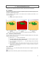
several fuel samples are necessary to build a vegetation object (See Figure 1). Fuel sampling is
generally carried out with the so called “cube” method (see above), collecting fuel in
elementary volumes of 25 cm side. Consequently a typical fuel sample is a 25 cm x 25 cm x
25 cm voxel, although it may have other dimensions. A fuel sample may be collected by field
destructive measurements (measured), or calculated.
Layer
Vegetation layer: layer composed of all the plants occupying the same vegetation
stratum: trees, shrubs and grasses layers are the main layers considered in this
document. Litter can be considered as a layer as well, but it is composed of downed
and dead woody debris.
Fuel Layer: collection of individual plants, closely grouped and difficult to describe
separately, forming a layer generally much more wide than high. A fuel layer is
described as a single vegetation object and has almost the same properties than an
individual plant. Each Fuel Layer is described with its own macroscopic properties,
including bulk density, LAI, moisture, cover fraction and characteristic size of clumps.
Quercus coccifera shrubland is a typical fuel layer.
Fuel LayerSets: A Fuel LayerSet is a polygon which contains different fuel layers,
which represent each fuel type included in the Fuel LayerSet. For example, a Fuel
LayerSet of garrigue, can contain 3 layers: Quercus coccifera, Rosmarinus officinalis
and Brachypodium retosum.. Fuel layers correspond to a fuel complex where few
information is available on the position of the individual fuel type inside of it or when
the user wants to summarize them in a unique object. It is generally used to
represent understorey, but can be also used to represent canopies.
Object: (Sensus CAPSIS) elements composing a scene such as a terrain, a grid, polygons,
polylines or vegetation objects (in other word item).
Plant: vegetation object
Measured plant: vegetation object corresponding to a real plant measured in the field.
Virtual plant: vegetation object not corresponding to real plant measured in the field. It may
differ either by its shape, by the distribution of cubes within its shape, by the values of one or
several fuel parameters (e.g. mean of several samples).
Renderer: (Computer science term) graphical way to represent a 3D object. FIRE PARADOX FUEL
MANAGER proposes several renderers to visualise Objects (terrain, grid and vegetation objects).
8
Terrain: ground surface of a vegetation stand. It may be flat or may follow the ground surface
topography through a Digital Elevation Model (DEM). This object is necessary to display
vegetation objects.
Shape pattern: characterization of the crown envelope of a vegetation object by defining the
ratios between the different horizontal stratifications of the crown.
Site: location where destructive fuel sampling has been carried out to characterize individual
plant or particle fuel properties.
Taxon: a taxon (plural taxa), is a name applied for an organism or a group of organisms. In
biological nomenclature according to Carl Linnaeus, a taxon is assigned to a taxonomic rank
and can be placed at a particular level in a systematic hierarchy reflecting evolutionary
relationships.
Team: Fire Paradox partner involved in fuel description field and laboratory works.
Vegetation object: individual plant (tree, shrub, grass) or fuel layer represented on the
vegetation scene and fully described as a fuel in the FIRE PARADOX FUEL database.
Vegetation scene: collection of vegetation objects organized on a landscape including
possibly different vegetation layers (trees, shrubs, grasses and litter).
H e ig ht
Voxel: Elementary volume for fuel description. It is generally, but not necessarily, a volume of
25 cm side. A voxel is part of the fuel sample collected in the field when using the cube method
(see Fuel sample).
Top
Centre
Diameter
VF
VF
VF
VF
VF
VF
VF
VF
VF
Base
Vegetation object
Distribution of fuel
samples in a
vegetation object
Three fuel samples types used to build
the vegetation object
Figure 1: Vegetation object built with 3 types of fuel samples
9
1
INTRODUCTION
This document presents the functionalities of the application identified as an Integrated Product
under the name “FIRE PARADOX FUEL MANAGER (FPFM)”. This application results from the activities
of WP6.1 “Design, development, test and deployment of a fuel editor” within the Fire Paradox
project.
The main goal of the FIRE PARADOX FUEL MANAGER is to generate – with a user friendly manner –
fuel complexes in 3D in order to be used as input data for fire behaviour models. These input
files describe the composition and the structure of the fuel complex taking into account the
physical properties of various components of the different vegetation layers (trees, shrubs,
herbs and litter) composing the vegetation scene.
The FIRE PARADOX FUEL MANAGER also provides tools for managing a fuel database: adding,
updating and deleting fuels descriptions (location and dimension of vegetation objects and fuel
parameters for fire simulations).
The FIRE PARADOX FUEL MANAGER is also enabling to visualise effects of fire on trees and to
simulate vegetation succession after fire occurrence.
1.1
Fuel manager
The FIRE PARADOX FUEL MANAGER aims to be, on one hand, a management tool for manipulating
fuel complexes and on the other hand, an application that enables fire simulations and the
generation of vegetation post fire succession steps. A survey of available technologies has
identified a simulation platform, Capsis [2][3], dedicated to hosting a wide range of models for
forest dynamics and stand growth. CAPSIS is a project leaded by a joint research unit INRAAMAP (Montpellier, France). In a few words, CAPSIS is designed around a kernel which provides
an organizational data structure (session, project, scenario steps) and also generic data
descriptions (stand, tree, etc.). These descriptions can be completed in modules – one for each
model – which implement a proper data structure and a specific evolution function (growth,
mortality, regeneration, etc.) with a chosen simulation step.
The FIRE PARADOX FUEL MANAGER development team decided to join the CAPSIS project to benefit
from this practical, scalable and free platform which is adapted to forestry modellers, forestry
managers and education. Thus, we co-developed a new CAPSIS module – “Fire Paradox” – which
implements data structure and functionalities of the FIRE PARADOX FUEL MANAGER.
CAPSIS and FIRE PARADOX FUEL MANAGER are both written in JAVA language [4].
1.2
The Fuel Database
Data related to fuel descriptions are stored in a database with the purpose of designing a
European data and knowledge base on fuels (FIRE PARADOX FUEL database). WSL is the partner
in charge of implementing the FUEL database in the framework of WP3.3.4 “Design a database
for fuel and plant architecture”. The data structure has been designed in collaboration with
INRA partner.
The complete database structure will be described in D3.3-6 “Database of fuel characteristics”
(due date month 48). The FUEL database is also accessible through a web interface available on
the Fire Paradox Fire Intuition platform at http://www.fireintuition.efi.int.
10
2
TERMINOLOGY AND CONCEPTS
This chapter gives a list of terms used in this manual. A few concepts were already explained in
the glossary and deliverable D6.1-2 “Detailed definition of the data structure and functionalities
of the FIRE PARADOX FUEL MANAGER”.
2.1
Session, project, module, scenario
Session, project, module and scenario are CAPSIS concepts. A session can contain several
projects; so the user can open several projects in parallel. Each project is associated to a
specific module chosen at the beginning. A project always contains a root step, supporting the
initial stand of the simulation, either loaded from file or virtually generated. The user can create
different scenarios by alternating growth sequences calculated by the model and silvicultural
treatments.
2.2
Extensions
The simulated data can then be checked by using specific extensions (plug-ins) of the module
or others that are compatible with: viewers, graphics, intervention methods (including thinning,
pruning, fertilization, plantation, etc.) and export tools in various formats for closer analysis.
2.3
Objects
A scene can be composed of several objects such as a terrain, a grid and several vegetation
objects.
A Terrain corresponds to the ground of a vegetation stand. It may be flat or may follow the
ground surface topography through a Digital Elevation Model (DEM). This object is necessary to
display vegetation objects.
A Grid is a set of lines dividing the ground surface in squares. Grid can be useful to locate
vegetation objects in the vegetation scene.
Vegetation objects can be trees, shrubs and grasses which properties can be extracted from the
FIRE PARADOX FUEL database or described in files.
2.4
Taxonomic Levels
Taxonomy is the science of classifying organisms. The system used in the FIRE PARADOX FUEL
database is the Linnaean one, which breaks down organisms into seven major divisions, called
taxa (singular: taxon). Divisions are as follow: kingdom, phylum, class, order, family, genus and
species.
The classification levels become more specific towards the bottom and we will focus on the
genus and species one. As example, Quercus ilex and Quercus coccifera species belong to the
same genus Quercus.
Taxon: a taxon (plural taxa), is a name applied for an organism or a group of organisms. In
biological nomenclature according to Carl Linnaeus, a taxon is assigned to a taxonomic rank
and can be placed at a particular level in a systematic hierarchy reflecting evolutionary
relationships.
11
2.5
Shape Pattern
A shape pattern characterizes the crown envelope of a vegetation object by defining the ratios
between the different horizontal stratifications of the crown (Figure 2).
The following dimensions are expressed in percentage of the crown height:
•
Top of the crown = 100%
•
Base of the crown = 0%
•
Level of the maximum crown diameter is set by the user. This dimension is used
as an indicator and will be readjusted by the effective height (of the max.
diameter) of the vegetation object.
•
The maximum crown diameter is also defined as a percentage of the crown
length.
Levels can be defined in order to adjust the form of the envelope in both horizontal and vertical
directions. In that respect, the crown is divided into two parts, the upper portion (over the max.
diameter level) and the lower portion (under the max. diameter level). Intermediate diameters
can be added in these two portions. Each of these new diameters is described by two
parameters:
•
Horizontal direction: percentage of the max. diameter length
•
Vertical direction: percentage of crown portion height
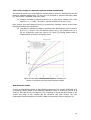
The Figure 2 illustrates a shape pattern which dimensions are:
•
Level of the max diameter is set at 30% of the crown height.
•
One intermediate crown diameter is defined at 50% of the height of the lower
part of the crown.
Figure 2: Shape Pattern with its dimensions
A vegetation object shape is succinctly described by its crown height, crown base height, max
crown diameter height and crown diameter length.
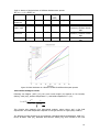
Figure 3 shows three different vegetation objects displayed by using the same shape pattern,
the one previously described in Figure 2.
12
14,7m (1)
14,1m (1)
12,3m (2)
11,3m (1)
11,1m (2)
6,5m (3)
6,1m (3)
8,9m (2)
6,5m (3)
9,7m (4)
5,8m (4)
4,4m (4)
Figure 3: (1) Crown height - (2) Max diameter height - (3) Crown base height
The first shape looks like its associated shape pattern (Figure 2), but the two others have quite
different aspects. It is due to one single property – the maximum crown diameter height –
which differs from one vegetation object to the other. Indeed, in the three illustrations, the
maximum diameter level is respectively 29%, 76% and 99% of the crown height, more or less
closed to the 33% set in the shape pattern.
To date, the maximum crown diameter height is randomly generated because this property is
still missing in vegetation objects description in the FIRE PARADOX FUEL database. This property is
planned to be filled in at the same time as other vegetation object shape properties thanks to
the vegetation object manipulation functionalities. The coherence between those different
inputs should be then guaranteed.
13
3
INSTALLATION AND CONFIGURATION
The installation and configuration of three components are necessary to fully use the FIRE
PARADOX FUEL MANAGER:
•
Java Runtime Environment (JRE), version 1.6
•
Module Fire Paradox of the CAPSIS platform.
Detailed instructions are given in the following chapters.
The FIRE PARADOX FUEL MANAGER works on Windows, Macintosh, Linux and anything else which
accepts Java. Steps dedicated to the Windows operating system are stressed in this chapter as
it is the most common operating system.
3.1
Java Runtime Environment installation
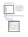
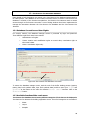
1- Install Java 1.6 (j2se) on your computer (Windows, Linux: see http://java.sun.com/j2se/,
Mac OS X: check that Apple's Java 1.6 is installed on your machine). You need a JRE (Runtime
Environment) for simple use or a JDK (Development Kit, including a java compiler) if you are a
developer.
2- Ensure that your PATH contains java_install_directory/bin/. You can check your PATH in a
new terminal by entering “java -version”.
If a JRE is already installed on your computer, a checkout will indicate the running version
number. Depending on the result, the required version will be installed.
In a terminal execute the following commands.
Windows
java -version
Linux / Mac OS X
sh java -version
Figure 4: Command window screenshot - java version 1.6 installed
3.2
Install & Start CAPSIS
CAPSIS is an open software platform which hosts a wide range of forests growth and dynamics
models. The “Fire Paradox” module, which has been developed within CAPSIS, corresponds to
the FIRE PARADOX FUEL MANAGER.
14
Many other CAPSIS modules exist but they are not released here. For further information,
consult the CAPSIS website (http://capsis.cirad.fr).
3.2.1
Download and Install
The installation file of the FIRE PARADOX FUEL MANAGER software (capsis-4.2.2-fireparadoxsetup_Feb2010.jar) can be downloaded from the Fire Paradox Fire Intuition platform at
http://www.fireintuition.efi.int
•
Double click on the capsis-4.2.2-fireparadox-setup_Feb2010.jar file
•
Follow the instructions
Figure 5: Installation of CAPSIS
On Windows Vista, you must choose a directory where you have write privileges (for instance
Documents)
3.2.2
Launch the CAPSIS Platform
Use the Start menu or the Desktop shortcut to start capsis
Change to capsis_install_directory\capsis4 directory and run the launcher script. CAPSIS
is available in French and English. To launch CAPSIS in French, use the “-l fr” option instead of
“-l en”, which stands for opening in English.
Windows
cd capsis_install_directory\capsis4
capsis
Linux
cd capsis_install_directory/capsis4
sh capsis.sh
NOTE: You can check CAPSIS option with the -h option
15
4
USE OF THE FIRE PARADOX FUEL MANAGER – OVERVIEW
In this chapter, an overview of the CAPSIS platform is first presented. Then, the way to use
available functionalities of the Fire Paradox module is described.
The items represented on a 3D vegetation scene can be used to build a large variety of
landscape, including zones with different fuel types. These items only contain the macroscopic
properties that are required for their representation and computation of mean fuel
characteristics at stand level (Table 1). These items are individual plants and Fuel LayerSets.
Fuel LayerSets are composed of several Fuel Layers (Table 2).
An individual plant can be a tree or a shrub, with a few characteristics including its dimension,
bulk density and LAI.
Fuel Layers correspond to fuel complex where few information is available on the position of
the individual fuel type inside of it or when the user wants to summarize them in a unique
object. This object is attached to a polygon of the scene, determining the location of the fuel
complex. It is generally used to represent understorey, but can be also used to represent
canopies. A Fuel LayerSet contains different Fuel Layers, which represent each fuel type
included in the Fuel LayerSet. For example, a Fuel LayerSet of garrigue, can contain 3 Fuel
Layers: Quercus coccifera, Rosmarinus officinalis and Brachypodium retosum. Each layer is
described with its own macrospopic properties, including bulk density, LAI, moisture, cover
fraction and characteristic size of clumps in the Fuel LayerSet. In the 3D editor, the individual
plants are represented as individual items, with a crown shape, whereas a Fuel LayerSet is
represented by a cylinder, which section is the polygon attached to the Fuel Layerset and the
height is the maximum of layer heights contained in the Fuel Layerset.
Table 1. Attributes of the main vegetation objects included in a vegetation scene
Scene items
- Terrain
- Grid
- Plant
- Fuel LayerSet
- Polygon
Plant attributes
Identifier, SpeciesName
Position (x,y,z)
DBH, TreeHeight, Crown Base Height, Crown
Diameter,
MaxDiameterHeight,
CrownProfile,
CrownColor BulkDensity, Leaf Area Idex
Live/Dead and Leave/Twig Moistures
FireParameters
SeverityParameters
(Additional attributes for database plant: TeamName,
Checked, CloseEnvironment)
Fuel LayerSet attributes
Identifier
Polygon
Layers
Height, BottomHeight
Load, CoverFraction
Table 2. Attributes of the Fuel Layers included in the Fuel LayerSets
Fuel Layer attributes
• SpeciesName
• Height, BottomHeight
• Alive/Dead BulkDensity, Leaf Area Index
• CoverFraction, PatchSize
• Live and Dead Moisture
• Additional attributes for database layers: TeamName,
Checked, ID, dominance,EdgeBulkDensity, edgeLAI)
16
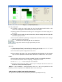
4.1
4.1.1
Screen Layouts
CAPSIS Screen Layout
Menu bar
Project name (‘Unnamed’) and Module name (‘Mountain)
Steps: root (0a) and treatment (*0a)
Stand Viewer,
Data displayer
View Panel
Figure 6: CAPSIS main window
General conventions are used in the CAPSIS user windows. The screen layout is composed of
several areas:
4.1.2
•
The menu bar allows access to the CAPSIS functionalities: new project creation,
etc.
•
An area gives a general overview of the current project: project name and its
associated module are indicated. The simulation history memorizes the root step
and other steps which result from growth evolutions or silvicultural treatments.
Each step has a date and holds a snapshot of the stand at this date, calculated
by the red model.
•
The left area presents all extensions of the platform that are compatible with the
module: charts, graphs, maps, etc.
•
The bottom-right space displays data according to the selected extension.
Module Fire Paradox Screen Layout
The 3D editor is designed to visualize and edit the scene containing the fuel. The main window
of the FIRE PARADOX FUEL MANAGER is divided into several functionally independent regions: a 3D
view panel of the scene (left), a menu bar, a tool bar and a real time control panel (right).
17
Tools Bar
3D View Panel
Real
Time
Panel
Control buttons
Figure 7: Main window of the FPFM
a) Tools Bar
This area composed of graphical icons, is dedicated to vegetation scene functionalities:
•
Camera toolbar buttons perform a number of viewpoint motions interactively
“Orbit” to change the orbit point of view
“Pan” to move the scene vertically and horizontally
“Zoom” to increase or decrease the focus
•
Scene modification functionalities:
“Select” to select an object on the scene
“Move” to move an object on the scene
“Add” to add an object on the scene
“Polyline” to draw a polyline
“Polygon” to draw a polygon
“Remove” to remove an object on the scene
“Undo” to cancel the last action
“Redo” to redo the last action
18
NOTE: All buttons, except “Polyline”, “Polygon”, “Add” and “Remove” are “sticky” buttons for
continuous selecting, panning, zooming, etc. The function of a sticky button you have clicked
on is remembered until you select another sticky button. If you select a non sticky button such
as the “remove” one after having selected an object; the FIRE PARADOX FUEL MANAGER will still
remember the previous sticky button function (the selected object is removed and you can
select other objects without having to click on “select” again).
b) 3D View Panel
In the middle of the window, the scene in 3D is displayed according to the current visualization
parameters.
c) Real Time Panel
The panel on the right is composed of several tabs which interact in real time with the 3D view
panel.
•
The “State” and “Selection” tabs display in real time information according to
the current scene including cover fraction, phytovolume of the understorey and
fuel load.
•
The “Scene” tab permits to list and see all objects displayed on the screen
(terrain, grid, polygons, trees).
•
The “Edition” tab permits to update precisely displayed objects coordinates.
•
The “Renderering” tab permits to modify visualization settings: the scene
representation changes automatically.
d) Control buttons
At the bottom, various buttons are available:
•
On the bottom left, a user right space and “Connection” button permit to access
to some functionalities according to the user profile (FIRE PARADOX FUEL database
management).
•
A “Patterns Editor” allows access to the vegetation pattern designer.
• On the bottom right, a few command buttons are available.
o “Previous/Next”: aims at navigating from generated scene and this main Fire
Paradox window.
o “OK”: validation of the vegetation scene; the Fire Paradox module is initialized.
o “Cancel”: the process is cancelled.
o “Help”: a user guide dedicated to the current window appears.
4.2
Keyboard Shortcuts
Keyboard shortcuts are indicated in square brackets: press simultaneously the combination of
keys to perform some tasks. This is a list of the most common keyboard shortcuts in the FIRE
PARADOX FUEL MANAGER.
Note that the [Escape] key close any CAPSIS window quickly; pay attention not to close an
important window by accident.
[Ctrl + N]
[Escape]
[Enter]
[Shift + Mouse click]
[Shift + Mouse hold down]
[Ctrl + Z]
[Ctrl + Y]
[Alt + R]
new CAPSIS project
close the window quickly
validate the window
multi-selection in selection mode
pan function in orbit mode
cancel last action
redo last action
orbit
19
pan
zoom
selection
move
add
polyline
polygon
remove
[Alt
[Alt
[Alt
[Alt
[Alt
[Alt
[Alt
[Alt
+
+
+
+
+
+
+
+
T]
Z]
S]
E]
A]
L]
P]
Del]
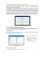
4.3
Program Help
Help buttons are available in the different dialog boxes in order to assist the user while working.
Figure 8: Example of CAPSIS help screen: inspector panel
20
5
5.1
VEGETATION SCENE CREATION
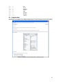
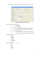
CAPSIS project creation
A project creation consists in initializing the root step of the Fire Paradox module under CAPSIS
platform; in other words in creating the initial planting set. All manipulative functionalities,
which are already available, will be loaded with this stage.
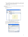
Click in the menu bar of the CAPSIS interface “Project > New” or [Ctrl + N]. The
following dialog window will appear.
Figure 9: New project window
Type a project name.
Select the model to be linked: “Fire Paradox”
Hit the “Initialize” button. Please refer to the chapter 5.2 for specific instructions.
Note: From this screen, you can also get documentation and information about FIRE
PARADOX model licence.
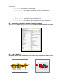
Figure 10: Example of Fire Paradox documentation page
21
5.2
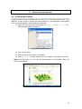
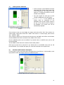
Vegetation scene creation
A scene can be created from text files of various formats containing the description of fuel in
terms of layers and can be edited and modified. Polyline and polygon can be added in the scene
as well as fuel items (plant, layerSet) with the “add” icon. A scene can be built from scratch,
only using “add” icon.
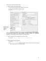
Several creation modes for generating a vegetation scene are currently available throughout the
user interface (Figure 11):
• From vegetation inventories: load an input file (database or detailed).
•
From field parameters: create a scene based on stand level characteristics.
•
From scratch: create an empty scene.
•
From a previous scene already saved for reedition
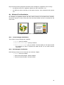
Figure 11: Scene generation window
The scene generation resulting from these different options, are detailed in the next chapters.
5.3
From a database inventory
This option enables to generate a vegetation scene by loading an inventory file which contains
only vegetation objects known in the FIRE PARADOX FUEL database. The inventory file describes
each vegetation object throughout its “ID” in the FIRE PARADOX FUEL database, and location. This
option requires a connection with the remote database since species, height and crown
dimensions are read for each fuel in the database before generating the scene. The inventory
file contains also a line describing the dimensions of the terrain. Using this option to generate a
vegetation scene will make possible the creation of export files necessary to run the fire
propagation model.
5.4
From a detailed Inventory File
A detailed inventory file can be loaded: it describes each vegetation object in details throughout
its species, crown dimensions and location. It doesn’t require an access to the FIRE PARADOX FUEL
database because it doesn’t contain vegetation object “ID” of the database.
5.4.1
For Viewing Only
This sub option is planned when user doesn’t need to run an export of the vegetation scene to
be able to run the fire behaviour model. It enables to display on the vegetation scene a wider
range of vegetation objects than those stored in the FIRE PARADOX FUEL database.
22
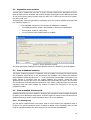
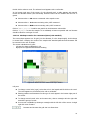
As example, an inventory file “Lamanon_Mixed_WP61_sg.scene” (cf. Annex 14.1) is available in
the given CAPSIS archive and precisely in the “capsis4\data\fireparadox” directory. The file
describes 48 trees.
Select the “From an Inventory” and “For viewing only” options of the scene
generation window.
Click on the “Browse” button and select the “Lamanon_Mixed_WP61_sg.scene” file in
the
“<install_directory>\capsis4\data\fireparadox”
directory
(e.g.
“C:\Program Files\capsis4\data\fireparadox”).
Click on the “Generate the scene” to display the resulting scene.
Figure 12: Scene creation from an inventory file
5.4.2
From POP COV files
This sub option enables to generate tree or shrub populations. Several populations can be
automatically generated by using some intra and inter populations spatial rules and constraints.
Spatial rules use the Gibbs parameter:
Gibbs parameter values: 0 = random distribution; 1000 = regular; <0 = aggregated
The vegetation scene has no link with the FIRE PARADOX FUEL database and cannot be exported
for running a fire simulation.
As example, an inventory file “_4REC_pop1Pins bonnes valeurs.txt” (cf. Annex 14.1) is
available in the given CAPSIS archive and precisely in the “capsis4\data\fireparadox”
directory.
Select the “From an Inventory” and “idem, .popcov files” options of the scene
generation window.
Click on the “Browse” button and select the ““_4REC_pop1Pins bonnes
valeurs.txt” file in the “<install_directory>\capsis4\data\fireparadox”
directory (e.g. “C:\Program Files\capsis4\data\fireparadox”).
Click on the “Generate the scene”
You can optionally modify values in the simplified dialog window untitled “Spatial
rules and constraints”.
5.4.3
From POP COV files Full Dialog
This sub option is similar to the previous one. The only difference is the display of a complete
dialog window for defining spatial rules and constraints.
23
5.4.4
For Matching with Database
This sub option is not available yet. It will be necessary when user will finally need to create an
export of the vegetation scene to be able to run the fire behaviour model. As the inventory file
doesn’t contain vegetation object “ID” of the FIRE PARADOX FUEL database, the loading procedure
will match each vegetation object with the most similar object present in the database.
5.5
From Field Parameters
This option is useful to generate automatically a vegetation scene, given some indications
describing its structure and composition. It may contain a list of dominant tree species (with
specific heights and DBH classes) and list of Fuel LayerSets including their respective Fuel
Layers for the description of the understorey (height, cover, bulk density, moisture content, …).
As an example, file “fuelbreak.txt” is available in folder capsis4/data/fireparadox (Annex 14.1).
5.6
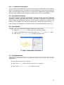
From Scratch
An empty scene can be generated by giving the dimensions of the terrain.
Select the “From scratch” option of the scene generation window.
Type the required dimensions (m) of the terrain in the “Length” and “Width” fields.
Click on the “Generate the scene” to display the empty scene.
Figure 13: Scene creation from scratch
5.7 From Saved Scene
CAPSIS can save FIRE PARADOX scene in a special format that can be re open later for further
modifications.
Select saved scene on your computer
Click on the “Browse” button and select the file in your computer
Click on the “Generate the scene” to display the scene.
24
6
VEGETATION SCENE MODIFICATION
Vegetation scene modification includes the selection, add and remove functionalities.
6.1
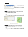
Selection
Individual and group selection techniques of vegetation objects are possible throughout the 3D
view panel in clicking with the mouse.
Selected vegetation objects appear in the chosen colour for selection (here RED) or in a
coloured bounding box.
to select an object on the scene
Figure 14: Vegetation objects
selection
Figure 15: Terrain object
selection
Figure 16: Grid object
selection
Note: While a selection is active, functionalities are effective only inside the selection
6.1.1
Individual or Multiple Selection
All type of objects visible on the scene can be selected: vegetation objects (tree, shrub, grass),
polygons, polylines, grid and terrain.
Click on the “Select” button of the Menu Bar.
For simple selection, click with the left-mouse button on desired vegetation objects.
This action deselects all previously selected objects.
For a multi-selection, hold down the [Ctrl] key while clicking with the left-mouse
button on objects.
For a selection of objects within a drawn area on the scene: move your mouse while
clicking with the left-mouse button and draw a rectangle including the group of
objects that you want to select.
6.1.2
Unselection
Hold down the [Ctrl] key while clicking with the left-mouse button on vegetation objects that
you want to unselect.
At any time the undo button, permit to cancel last actions, even selections.
25
6.1.3
Selection with the Scene Inspector
Object selection is also possible with the scene inspector.
Click on the “Scene” tab of the “Real
Time Panel”. All objects visible on the
scene will appear in the inspector.
For simple selection, click with the leftmouse button on desired vegetation
objects. This action deselects all
previously selected objects.
For a multi-selection, hold down the
[Ctrl] key while clicking with the
left-mouse button on objects.
Figure 17: Multi-selection of trees in the scene inspector
6.2
Adding
An interactive mode permits to add objects on the scene. This chapter focuses on the way to
display vegetation objects on the vegetation scene, and on the way to add figures as polygons
or polylines.
to add an object on the scene
Choose the vegetation object
Choose the planting method process
Click on “ADD” to add the object (s)
Figure 18: Dialog window for adding a vegetation object in the scene
26
The interface is divided into two areas dedicated to the selection of “what to add” (“Items
choice” frame) and the definition of “how to add” (“Spatialisation” frame).
6.2.1
Item choice: Vegetation Objects Selection
Two drop-down lists permit to indicate the object item to add in the following list:
• FireParadox Database Tree
• Local tree
• FireParadox Database Layer
• Local layer
For each type, selection criteria are displayed to help the user in his research. A table displays
available vegetation objects according to the criteria.
a)
Adding a FireParadox Database Tree
Fill the selection criteria if necessary
Select a Tree in the list extracted from the database
Add the selected tree on the scene with a planting option
Figure 19: Adding a Database Tree
b)
Adding a Local Tree
Select a tree species
Fill the tree general information
Add the selected tree on the scene with a planting option
27
Figure 20: Adding a Local Tree
c)
Adding a FireParadox Layer Sets (a Composite Layer from the FIRE PARADOX FUEL
database)
Select a Layer in the list extracted from the FUEL database
Click on “ADD” to add this layer to the composite layer
Update Layer description in the Composite Layer table
Repeat these action as far as the Composite Layer is not complete
Add the Composite Layer on the scene with planting option
Figure 21: Adding a Layer from the FUEL database
28
d)
Adding a Local Layer
A Local Layer Set is a Composite Layer built with layers that are not extracted from the FUEL
database. Local Layers may have tow origins:
•
“Predefined LayerSets”: The button “Add layerSet” entails to add the layers of
predefined layerSet models. Other default models can be added in a text file if required.
Note: The option for evolution with time is not yet available.
•
“Build the LayerSet from individual layers”: The button “Add layer” entails to
add selected layers one by one.
Note: All the layers included in the “Local Layer Sets” can be edited and modified if the user
prefers specific values for a given parameter in the table.
Figure 22: Adding a Local Layer
6.2.2
Spatialisation: Planting Method Process
The planting process is the way to display vegetation objects on the vegetation scene. After
having selected a vegetation object, it is necessary to specify its location, its clone number and
its planting structure.
Different modes for spatial display of vegetation objects on the scene are currently available:
Interactive planting
Planting along a line
Planting in rows
Random patterns
29
a) Interactive Planting
This option enables to locate trees directly on the scene, with the mouse.
When this option is activate, one vegetation
object will be planted for each click on the
scene.
It is possible to deactivate this option, for
selecting functionality or any other object on
the scene.
Figure 23: Interactive planting dialog
b) Along a line
This function permits to plant vegetation objects along a line according to spatial parameters.
A line can be a polyline or the contour of a polygon.
A “Number of items” or a “Density” per meter can be displayed on the scene.
“Absence probability” enables to specify a rate of exceptions in the planting
process.
“Alea” is the maximum distance that is permitted between the selected line and the
effective location of the planted object.
Figure 24: Along line planting process
c) Planting in rows
This function permits to plant vegetation objects in rows according to spatial parameters.
Planting can be done on the all scene or only “Inside a selected polygon”.
“Distance between plants” and “Distance between rows” determine the planting
pattern.
“Absence probability” and “Random” enables to specify a rate of exceptions in the
planting process.
30
Figure 25: Planting in rows method of planting
d) Random Patterns
This function permits to display a set of vegetation objects following a random pattern.
Planting can be done on the all scene or only “Inside a selected polygon”.
“Number of items” determines the number of trees that will be randomly generated.
Figure 26: Random pattern method of planting
6.2.3
Adding a Polygon or a Polyline
It is possible to add vegetation objects (individual plants) within or along a polyline or a
polygon. The application offers tools to add polylines or polygons on the scene.
to draw a polyline
to draw a polygon
Click on the right icon and draw the figure with you mouse.
A double click enables to end the drawing. For a polygon, the figure will be closed
automatically.
Figure 27: Drawing a polyline
Figure 28: Drawing a polygon
31
6.3
Updating
The scene structure can be modified by moving vegetation objects on the scene. Several
vegetation objects can be moved simultaneously thanks to a multi-selection process.
Silvicultural treatments, in other word the modification of the vegetation structure on a
predefined scheme (tree thinning, brush clearing, etc.), are available as an “Intervention”
once the scene has been validated (see Chapter 10).
6.3.1
Moving Functionality
Select vegetation object(s) to be moved.
to move an object on the scene.
Hold down the left-mouse button while moving the cursor to the target location.
The “Edition” tab also permit to update precisely selected objects coordinates.
Select vegetation object(s) to be moved.
Select on “Edition” tab of the “Real Time Panel”.
Change the object coordinates
Figure 29: Tree coordinates edition
6.3.2
Figure 30: Grid coordinates edition
Deleting Functionality
The suppression is available on pre-selected vegetation objects.
Select vegetation object(s) you want to delete.
to remove the object on the scene.
32
7
7.1
VEGETATION SCENE VISUALISATION
Viewpoint Motions
View motion functions allow the user to interactively rotate, zoom and pan the vegetation
scene.
Note: x-axis (horizontal) as direction of fire propagation, z-axis as vertical direction and yaxis as the depth of the scene.
7.1.1
Orbit Functionality
3D orbit motion permits to change the user viewpoint while keeping the target scene fixed.
Click on
“Orbit” button of the Menu Bar.
Hold down the left-mouse button and drag in the 3D view panel:
Drag up/down to rotate the scene around the x-axis,
Drag left/right to rotate the scene around the z-axis.
Figure 31: Angular, side and bird’s eye views obtained by orbit view motion
7.1.2
Zoom Functionality
The zoom function moves the viewpoint either further from (zoom out) or closer to (zoom in)
the vegetation scene. Two ways are available:
Click on
“Zoom” button of the Menu Bar.
Hold down the left-mouse button and drag in the 3D view panel:
Drag up to zoom out,
Drag down to zoom in.
7.1.3
Pan Functionality
The pan functionality is useful to crop the view as it moves the scene while keeping the
viewpoint fixed. Two ways are available:
Click on
“Pan” button of the Menu Bar.
Hold down the left-mouse button and drag the cursor in the desired direction.
33
7.2
Object Renderers
Objects (terrain, grid and vegetation objects) of the vegetation scene can be visualized in
different ways thanks to several renderers.
As any renderers are in fact CAPSIS extensions, the Fire Paradox module needs only to match an
extension to be able to use it. So, “Bounding Boxes”, “Lollypops” and “Grid” renderers are
used as they were released in CAPSIS; it implies to adapt some functionalities to the FIRE
PARADOX FUEL MANAGER requirements. On the contrary, the “Pattern Sketcher” renderer was
especially developed for the FIRE PARADOX FUEL MANAGER purposes.
7.2.1
Renderers Dialog Windows
Renderers can be user-configured in the “Rendering” tab of the “Real Time Panel”. The tab
is composed of two frames:
•
The “Renderers list” at the top
displays all objects (terrain, grid and
vegetation objects) which are contained
in the scene with an associated render.
•
The “Settings pane” permits to edit
settings which are specific to each kind
of render. For instance, if vegetation
objects are displayed with the lollypop
render, the user can change the
settings for the crown representation.
Figure 32: Object renders panel
Right-click on an object item of the “Renders’ list” to change its current render
with one of the available ones.
In the corresponding “Settings pane”, you can modify its parameters.
Figure 33: Tree bounding boxes render
Figure 34: Tree lollypop with profile render
34
7.2.2
Pattern Sketcher Render
A “Pattern Sketcher” render has been created especially for the FIRE PARADOX FUEL MANAGER.
Dedicated to vegetation objects, this render permits to visually differentiate categories of
vegetation objects using geometric forms and colours. Please refer to the specific “Patterns’
Editor” (chapter 9) to know more about editable functions.
Various geometric shapes of the tree crowns may be used to display various tree species or
different height classes of the same species. A colour setting enables further details in
vegetation classification display.
The “Settings pane” dedicated to the “Pattern Sketcher” render is divided into two main
panels.
a) “Colors” frame
This frame contains four options and a table. According to each option, the table content differs
and the user can set colors to different targets. Setting colors in function of criteria permits to
visually analyse the scene (chapter 8).
b)
•
“One color” option: set a unique color to all vegetation objects of the scene
•
“By taxon” option: set different colors for each taxon of the scene.
•
“By height threshold (m)” option: set a color to shape patterns according to a
height threshold. Fill in a value in the corresponding field and validate by pressing
the [Enter] key.
“Rendering” frame
This frame reused similar functionalities – visible/invisible and filled/outline options – as for the
lollypop render. Two additional options are proposed:
Untick the “Flat” option to display shading effects.
The “Light” option permits to switch on/off the light which illuminates the scene.
The use of this parameter is dedicated to the fire damage visualisation; please refer
to chapter for further details.
Figure 35: Pattern Sketcher Render options
35
7.2.3
Degraded modes for heavy scene manipulation
Special attention has been paid to the robustness and efficiency of scene manipulation, because
3D visualization is a costly technology and items displayed on the vegetation scene can be very
numerous.
First, a degraded mode based on skeleton of tree crown is used by default during view
manipulation (fast mode).
Second, the rendering of trees is degraded when tree number is high (Table 3), so that scene
manipulation is maintained. The quality of this representation can be temporary increased for
more accurate visualization.
Table 3. Rendering mode by default depending of the number of trees
Tree number
<=20,000
<=150,000
>150,000
Rendering
Crown and trunk plotted, hyperbolic decrease
of the number of sectors use for crown
representation from 16 to 4
Crown plotted only, 4 segments only for crown
representation,
for
the
highest
trees;
anchorage only for the smallest; the proportion
of trees represented by their anchorage
increase linearly with the tree number
All trees represented by default by their
anchorage (number of pixel depending on tree
size)
Quality note
Between 50 and 100 %
Between 1 and 50 %
1%
To increase rendering level of the “Pattern sketcher” of trees can be improved or degraded
manually through the parameter “Scene quality note”, with can vary from 0 (worse
resolution) to 100 % (best representation).
36
8
VEGETATION SCENE ANALYSIS
Descriptive analysis is available in the “Real Time Panel” on the right side of the FIRE PARADOX
FUEL MANAGER main window (Figure 7). Analysis can be made on the whole set of vegetation
objects or limited to a subset. In addition, visual analysis refers to different displays of the
vegetation objects in the 3D panel.
In addition to relevant statistics, vegetation scene screenshots will give a visual overview of the
vegetation scene.
8.1
Descriptive Analysis on the whole set of Vegetation Objects
The “State” tab of the “Real Time Panel” is dedicated to the analysis of the whole set of
vegetation objects. The aim is to display in real time indicators relative to the vegetation scene
composition and structure. It aims at helping user to follow-up the construction of the scene
and to compare its current state to initial objectives: cover, presence of dominant species, etc.
Figure 36: Descriptive analysis, State panel
The indicators available are:
a) General
•
“Total cover (%)”: total cover fraction of the vegetation displayed on the scene
•
“Maximum height (m)”: height reached by the highest vegetation object.
•
“Total Load (kg/m2)”: total fuel load (only fine fuel)
•
“Number”: the number of vegetation objects present on the scene.
b) Threshold between trees and shrub
•
“Threshold value (m)”: vegetation objects lower than the threshold value
belong to the shrub strata, whereas others belong to the tree strata.
37
c) Tree stata
•
“Cover %”: cover fraction of the tree strata
•
“Load (kg/m2)”: fuel load of the tree strata (only fine fuel is considered).
•
“Number” of vegetation objects in the tree strata.
d) Shrub stata
8.2
•
“Cover %”: cover fraction of the shrub strata
•
“Phytovolume”: bulk volume of shrub strata (m3/ha)
•
“Load (kg/m2)”: fuel load of the shrub strata (only fine fuel is considered).
Descriptive Analysis on Selected Vegetation Objects
The “Selection” tab in the “Real Time Panel” permits to display information on selected
vegetation objects. The tool called “Inspector” displays detailed data on the selected object.
Figure 37: Tree Inspector Panel
8.3
Visual Analysis
During the Pattern render development, some options were developed in addition such as
setting colours to shape patterns according to criteria species or height threshold.
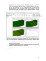
11m
Figure 38: By height threshold
Figure 39: By species
38
Figures 38 and 39 show perspective and side views to display the vegetation scene in using:
•
two different colours for vegetation objects over and underneath 11 m.
•
two different colours according to the species criterion, Pinus halepensis and Quercus
ilex .
8.4
Effects of Fire Visualisation
Fire damage on vegetation objects has been mainly focused on fire-induced tree mortality.
Several fire impacts on trees crown and trunk have been defined and can be visualized at the
scene scale.
Figure 40: Visualisation of fire impacts on trees
8.4.1
Crown Damages visualisation
Three levels of crown damages are classified:
• “Crown”: green per default.
• “Crown scorched height”: yellow per default.
• “Crown killed height”: grey per default. The best display of this impact would
be transparent in order to represent the dead fuel but it is too much resource
consuming.
8.4.2
Bole Damages visualisation
Bark charring is shown on tree trunk with min. and max. heights.
• “Trunk”: brown per default.
• “Max trunk charred height”: dark per default.
• “Min trunk charred height”: dark per default.
39
8.5
Visualisation Options
For Pattern sketcher render, several visualisation options are available:
•
Trunk visible (Yes/No)
•
Crown visible (Yes/No)
•
Crown filled or outlined
•
Crown flat (Yes/No)
•
Light (Yes/No)
Figure 41: Various visualisations options of pattern sketcher render
40
9
PATTERNS’ EDITOR
The crown Patterns’ Editor enables to create shape patterns and to assign those typical crown
profiles to groups of vegetation objects. Three criteria are taken into account – taxon, height
and environment (openness: open/closed environment) – to constitute groups of vegetation
objects. Crown overall structure depends strongly on these three criteria.
Click on the “Patterns’ Editor” button in the “bottom toolbar” to access the
Patterns’ Editor and its functionalities (please note that it takes a few seconds to
open the Patterns’ Editor for the first time).
9.1
Screen Layout
The Patterns’ Editor main interface gives an overview of available associations between criteria
and shape patterns. Advanced functionalities can be accessed throughout the different areas of
this dialog window.
Note: Several interfaces deals with shape patterns; an overview of links is displayed in
Annex 14.2.
Association
Criteria
Pattern List
Associations
Criteria –
Shape
Pattern
Previewer
Function buttons
Figure 42: Main window of the Patterns’ Editor
a) Frame “Filter”
The frame “Filter” permits to sort all available associations using the three criteria: taxon,
height interval and environment. Check a box in front of a criterion to filter the associations.
The “Taxa” drop down list contains all taxa stored in the FIRE PARADOX FUEL
database.
o Select a genus or species to sort associations mentioning it.
o Check the “Strict” box to make a search on association with the right taxon.
o Unchecking it lets the search performed on the right taxon and less taxonomic
level (e.g. criteria = Quercus; associations with Quercus and related species are
searched – Quercus ilex, etc.).
•
•
The “Height interval (m)” contains two fields dedicated to the lower and
upper limits of an interval, respectively inclusive and rejected values.
41
Fill in a value as lower limit to search all associations which is higher.
Fill in a value as upper limit to search all associations which is lower.
Fill in values as lower and upper limits to search all associations which height is
included in the specified interval.
Note that associations with no specified height interval display all the possible
results.
o
o
o
•
The “Environment” drop down list contains two values: open and closed.
b) Frame “Criteria/Pattern links”
•
Table
This frame displays available associations between criteria and shape patterns. Each line of the
table is an association: the first three columns correspond to the criteria and the last one
indicates the associated shape pattern name.
Associations of the table can be sorted by column entitled by clicking on.
•
Buttons
Manipulative functionalities are available throughout the “Add”, “Remove” and “Modify” buttons.
o
o
o
Create an association: refer to chapter 9.2.1.
Update an association: refer to chapter 9.2.2.
Delete an association: refer to chapter 9.2.3.
c) Frame “Preview”
A preview of the selected shape pattern is displayed at the right side of the interface. Inferior
and superior areas are displayed as well as the dimensions of each crown diameter.
A problem subsists in the shape pattern proportions: as the crown is expressed in percentage;
it should be a cube and remain a cube when the window is re-size computer.
d) Patterns’ List
At the bottom right of the window, a “Patterns’ List” button permits to have access to a
dialog window dedicated to available shape patterns; refer to chapter 9.3.1.
9.2
Association: Shape Pattern linked to a Group of Vegetation Objects
A shape pattern is supposed to be created in the purpose of being used by a group of
vegetation objects. That’s why criteria are specified in a first time to identify a collection of
vegetation objects for which a shape pattern is then assigned.
According to the taxon, height and environment criteria, each vegetation object should have a
reference shape pattern.
42
The dialog window designed to associate criteria to a shape pattern is composed of three areas:
•
The “Criteria” area displays the three criteria which can be filled in.
•
The “Patterns” area offers three options to choose a shape pattern.
•
The “Preview” area is the same as described in the previous dialog box.
Figure 43: Add and update association window
9.2.1
Create an Association
It is forbidden to create similar associations using the same taxon, height intervals and
openness.
Click on the “Add” button of the Patterns’ Editor main window.
Fill in the right criteria. The “Taxon” one is mandatory.
Associate a shape pattern to the criteria:
An existing one: select an available shape pattern in the drop down list.
A new one: click on the “Create” button to create a new shape pattern;
A clone one: select an available shape pattern in the drop down list and click
the “Clone and edit” button. This option is useful to create a new shape
pattern based on an existing one.
Validate by clicking “Confirm”; the new association is added to the table.
9.2.2
Update an Association
Updating an association consists in updating the criteria and/or updating the associated shape
pattern. Those modifications imply to take into account the same coherence rules as for a new
association.
Select an association in the table.
Click on the “Modify” button of the Patterns’ Editor main interface to open the same
window as for adding an association. The parameters of the selected association are
already filled in and can be modified.
Validate your changes by clicking the “Confirm” button.
9.2.3
Remove an Association
Associations can be removed by two ways:
a) “Remove” button
Select an association in the table.
Click on the “Remove” button of the Patterns’ Editor main interface to delete the
current association. The user must confirm before really removing the association.
43
b) “Reset” button
At the bottom left of the interface, the “Reset” button permits to delete all “client” associations.
9.3
9.3.1
Shape Patterns
Shape Patterns Dialog Windows
Two dialog windows enable to manage shape patterns. The first one permits to describe a
shape pattern and the second one is listing all available shape patterns.
Figure 44: Shape patterns edition window
Figure 45: List of available shape patterns
a) Shape Patterns’ List Window:
•
“Patterns’ List” frame
o A list of available shape patterns is displayed.
o The “Remove patterns” button permits to delete a pre-selected shape
pattern.
o The “Edit patterns” button permits to modify the shape pattern
description.
•
The “Preview” frame, displayed on the right side of the window, gives an
overview of the selected shape pattern.
•
The “Reset” button permits to delete all associations.
b) Shape Pattern Edition Window:
•
The “Information” frame contains several data to identify clearly each shape
pattern:
o A “Key” as a single identifying.
o A “Name” composed of an alias – if any, a shape pattern number and
some information on crown diameters (e.g. “JUNI-15-30-s80” means
that the alias is JUNI; the pattern number is 15; the max diameter
height is at 30% of the crown height and an intermediate diameter is
set at 80% of the superior area).
o An optional “Alias” can be given to each shape pattern for a better
readability.
•
The “Max diameter height” field contains the max diameter height. Per default,
it is set at 50% of the crown height.
•
“Superior diameters” and “Inferior diameters” frames are structured in the
same way:
o Two fields are dedicated to set the intermediate diameter parameters:
the diameter height position in the crown (%) and its length
proportionately to the max diameter.
44
o
o
o
9.3.2
The “Add” button permits to create the new diameter according to its
parameters.
A table summarizes all intermediate diameters.
The “Remove” button permits to delete a pre-selected intermediate
diameter.
•
A “Preview” frame is displayed on the right side of the window to give an
overview of the shape pattern during its construction.
•
The “Reset” button permits to reset the parameters as it was at the beginning
(without warning).
Create a Shape Pattern
A shape pattern can only be created during the creation process of an association.
Click on the “Create” button.
Give an alias (optional) to the shape pattern. The key and name data are
automatically generated.
Modify the max diameter height and press the [Enter] key to validate.
Add intermediate diameter in the superior and/or inferior areas of the crown by
filling in the corresponding parameters. Click on the “Add” button or press the
[Enter] key to validate. The table is automatically refreshed. Columns of the table
are editable in double-clicking values; press the [Enter] key to validate.
Press the “Ok” button to validate the shape pattern description.
9.3.3
Update a Shape Pattern
Knowing first the shape pattern to update, go to the right interface throughout the one
displaying all shape patterns.
Click on the “Edit patterns” button to open the same interface as for a shape
pattern creation.
Modify all the necessary parameters (alias, intermediate diameter dimensions, etc.)
and validate by clicking the “Ok” button.
9.3.4
Delete a Shape Pattern
A pattern shape can’t be suppressed if it is used in an association.
From the “Patterns’ list” window, shape patterns can be removed by two ways:
a) “Remove Pattern” button
Select a shape pattern in the list.
Click on the “Remove Patterns” button to delete the selected shape pattern.
Validate the confirmation dialog box.
b) “Reset” button
At the bottom left of the interface, the “Reset” button permits to delete all shape patterns.
45
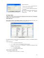
10 STAND EVOLUTION AND INTERVENTIONS
When a vegetation scene is ready (Figure 47), it can be validated with the “OK” button of the
scene editor panel and it becomes an initial step (0a) (root step). From this initial step, an
various evolution scenarios can be run.
Figure 47: An example of ready to validate vegetation scene
CAPSIS hosts models for forests / plantations growth and dynamics modeling. All modules,
including the FIRE PARADOX MODULE can be run under the same framework. Under a given
project, different simulations can be run to investigate several scenarios of the life of a stand.
Each simulation history contains different steps to describe stand evolution, human
interventions and ecological perturbations. Projects memorize the different steps of the
simulation history. Each step has a date and holds a snapshot of the stand at this date,
calculated by the linked model. A simulation always contains a root step, supporting the initial
stand, either loaded from file or virtually generated. When the project is initialized (i.e. model
parameters are set and initial stand is loaded), it appears in the Project Manager interface
(Figure 48). A header shows its main properties (name, model name, surface…) and the initial
stand (0a) is linked to the root Step with a date. The Project Manager provides a Step
contextual menu (the Step Menu) which contains Step management options.
Figure 48: CAPSIS project manager interface, with the step contextual menu displayed
46
When you click on a step (left button), it becomes the Current Step (with a pressed look) and
the project becomes the Current Project (with a project selection color). Actions in the Project
menu occur on the current project.
10.1 Project configuration, saving and opening
Open the Project Configuration dialog
Select the project by left-clicking one of its steps
Project > Configure
•
Change the project name
•
See more or less steps in the Project Manager
•
Watch the settings of the CAPSIS model linked to the project
Projects can be saved on disk and reloaded later on in the same exact state. The linked model
is also saved with its current settings in order to be reusable after re-opening.
To save a project on disk:
•
Select the project by clicking on one of its steps
•
Project > Save As
•
Choose a location and file name (free file extension)
•
Validate
To open a project from disk:
•
Project > Open
•
Select the file containing the project in the file system
•
An overview shows information of the selected project / file
•
Validate
10.2 Groups
Some models manage individual trees or plot cells in their data structure. For these models, it is
possible to create groups of trees or plot cells. These groups can be named and then used in
the Viewers (ex: restrict to trees higher than 10m) or in graphical outputs.
To open the “GROUP” catalog
•
StepMenu > Group
Create a new “GROUP”
•
Group catalog > New
•
Choose a name for the group
•
Choose group type (ex: Trees / Dynamic)
•
Select a filter
•
Parameterize it
•
Inspect the result in the display
•
Optionally refine selection with other filters
•
When everything is ok, Validate
47
The group is saved to disk, it is now known by CAPSIS until it is removed from the catalog.
Customize a “GROUP”
•
Group catalog
•
Select a Group to be customized in the list
•
Customize
•
Change filters parameters
•
Validate
Remove a “GROUP”
•
Group catalog
•
Select a Group
•
Delete
10.3 Stand intervention
Among the management options, the user can choose:
•
to compute an evolution of the stand from a given step for a given number of
years: “EVOLUTION” (this functionality is detailed in the main CAPSIS help on
line),
•
to compute an intervention (pruning, thinning, clearing, etc.) or a perturbation
(Fire effects, etc.): “INTERVENTION”,
•
to export the current step in a given format: “EXPORT” (this functionality will be
detailed in the next chapter).
In the case of an “EVOLUTION”, the model calculates different steps and links them after the
starting step. These new steps will have different dates. In the case of an “INTERVENTION” the
user has to parameterize the “INTERVENTION”. A new step is added after the chosen step,
carrying the stand after “INTERVENTION” (Figure 49).
Viewers can give a representation of the stand under a given project step. This representation
can be graphical (maps, distribution) or not (text). Graphical outputs can mix data extracted
from several steps of one or several projects. These representations can be graphical (curves,
histograms, scatter plots…) or not (tables, text…).
10.3.1 Interventions
Fire managers use mostly thinning and pruning, as canopy fuel treatment. Among the variety of
thinning possibilities available in CAPSIS, it is possible to simulate a thinning that respaces stems
or crowns. It is thus possible to simulate fuel-break according to French recommendations (ie, a
distance of 3 m between crowns). Pruning is also available. Generally, interventions are applied
to a group of trees or to a spatial location, which can be defined with a variety of criteria. For
example, the fuel-break presented on Figure 49 was build with a respacing of crowns at 3 m
from an initial stand with 800 stem/ha.
10.3.2 Fire perturbation
Fire perturbation is a specific case of “INTERVENTION” on the vegetation stand. This
functionality enables to calculate the fire impacts on the vegetation objects and namely on
trees. Two main options are available:
• Using the outcomes of the FIRETEC fire propagation model. This option requires
exporting first the vegetation scene in order to run a FIRETEC simulation (see next
chapter). The result of a fire spread in terms of fire effects can be computed, as a
48
•
function of different parameters (intensity and residence time, rate of spread and
residence time, etc.). It results in a new step or scenario in stand life.
Using some published empirical models relating fire behaviour parameters to fire effects
on trees. This second option is the only one presented below. The empirical models
described below can thus be used to assess the fire severity parameters of each tree
(crown scorch/kill height and volume, cambium damage probability, mortality
probability, etc). The user can select the empirical model he wants for crown damage,
cambium damage and mortality probability through combo boxes.
Figure 49: Project manager with 3 scenarios in an Aleppo pine stand separated by a road (in
black). The top part represents the different steps in year in the different scenarios, starting
from a same initial stand (0a), visualized below (top left 3D viewer). The different scenarios
are:
• a: natural evolution during 6 years of the stand,
• b: understorey clearing and tree thinning (5 m between crowns) on a 100 m wide zone,
followed by 6 years of evolution
• c: understorey clearing and tree thinning (5 m between crowns) on a 100 m wide zone,
followed by 3 years of evolution and a fire (750 kW/m)
Damage from the fire can be seen on bottom left 3D viewer, as well as some statistics on the
tree that died (in red), compared to their original number (in blue), by class of diameter
(bottom right).
49
10.3.2.1 Fire damage to cambium (empirical models implemented)
Two empirical models can provide cambium mortality criterion, based on bark thickness and fire
behaviour standard characteristics. The first one was proposed by Peterson and Ryan (1986)
[5], derived from a simplified conduction model:
Cambium mortality is assumed and the tree is killed when residence time (min)
superior to t kill
= 2.9BT 2 , where BT is the bark thickness of the tree (in cm).
More recently, Bova and Dickinson (2005) [6] proposed the following criterion, derived from
dimensional analysis and experiments:
Tree death by cambium mortality is considered when bark thickness (mm) is lower to
0.2 I 0.20τ 0.64 , where I is the fire intensity (kW/m) and τ the residence time (s) of
the fire. Preliminary works with Jones et al. (2004) [7] physical models seem to
compare better to Peterson and Ryan’s model.
Figure 50: Bark thickness threshold for cambium mortality as a
function of residence time with several empirical models
Bark thickness models
A review of relationships available for bark thickness assessment as a function of DBH was done
for European species, based on the following publications (Ryan et al 1994 [8]; Pimont et al
2006 [9]; IFN 1990-04 [10]; IFN 1990-06 [11]). A selection of models was done, based on the
number and range of tree sampled and the coherence with other models. The main
relationships of bark thickness as a function of DBH are presented in Table 4 and Figure 51.
50
Table 4: Review of bark thickness of different Mediterranean species
BT (m) = a + b × DBH c (m)
Species
References
Origin
1
R2
(#
trees)
0.99
[8]
8-84 cm
0.067
0.0621
1
0.838
0.75
(2371)
[8]
[10, 11]
0
0.0381
0.623
(3218)
[10, 11]
0
0.0232
0.614
(288)
[10, 11]
8-60 cm
8-60 cm Alpes de Haute
Provence, Southern French
Alps
8-70 cm Alpes de Haute
Provence, Southern French
Alps
8-35 cm Southern French
Alps
A
b
c
0.000424
0.076
0.00559
0
Quercus
pubescens
Quercus ilex
Pinus
halepensis
Pinus pinea
Pinus nigra
subsp. nigra
Figure 51: Bark thickness as a function of DBH for different European species
10.3.2.2 Fire damage to crown
Following Van Wagner (1977) [12], the crown scorch height (m) depends on fire intensity
(kW/m), wind (m/s), ambient temperature Tair, and lethal temperature Tcrit (°C):
h = 4.55
I2/3
(Tcrit − Tair )
1
1 + 38
U3
I
This formula was obtained from dimensional analysis, plume theory and a few field
experiments. The lethal temperature depends on the type and size of organ (buds, needles).
The different models derived from this approach (Saveland and Neuenschwander 1989 [13],
Finney & Martin 1992 [14], Michaletz and Johnson 2006a [15]) were included in the FUEL
51
MANAGER. The assessment of scorch or kill height is used in the software to compute the crown
volume scorched (Figure 52), required for mortality models, assuming a crown shape [5] or
detailed plant architecture.
Figure 52: Simulated damage to bole and crown in a Pinus halepensis stand, assuming a fire
intensity of 1000 kW/m and a residence time of 1 minute.
10.3.2.3 Tree mortality
A large variety of mortality models has been developed for European species (Table 5). These
models were implemented in the FUEL MANAGER, using Crown Volume Scorched and Bark
Thickness derived from the model described above. Additional mortality resulting from cambial
damage was also computed based on cambium damage criteria.
Other models that integrate more directly the mechanisms involved in death were also
implemented:
τc
CVK τ − 0.5
Pm =
100
, with CVK the crown volume killed (%), τc the critical time for cambium
mortality and τ, the residence time [9].
More recently, Michaletz & Johnson (2008) [16] have proposed the following model by including
more processes:
N n δ (x c ,BT )
Pm =
Nt
, with Nn and Nt, respectively the number of killed buds and the total number
of buds, xc the maximum necrosis depth in bark, BT the bark thickness (δt=1 if t>=1, else 0).
In this last model, the pipe model assumption is used to evaluate Nn/Nt with 1- SAn/SAlcb, SA
(sapwood area), evaluated with allometric relationships.
52
Table 5: Mortality models available for a few Mediterranean species
P = [1 + exp (b0 + b1 x1 +…+ bk xk)]-1
Species [Source]
P. halepensis [17]
P. nigra subs. laricio [9]
P. pinaster [18]
P. pinaster [9]
P. pinea [17]
P. sylvestris [19]
Generic [20]
Variables and coefficient
b0
b1 x 1
b2 x 2
1.75
-0.0385 CVS
-2.01
-0.0004 CVS2
4.17 (1-e-BT)
2.32
-0.00038 CVS2
0.1119 DBH
-1.13
-0.118 BLC
8.78 (1-e-BT)
-0.222
-0.103 BLC
9.95 (1-e-BT)
7.390
-0.101 CVS
0.00381 DBH
0.527
-3.53 BCmean
9.04 (1-e-BT)
-0.773
-0.0679 BLC
5.39 (1-e-BT)
0.759
-0.0499 BLC
9.32 (1-e-BT)
23.0
-0.253 CVS
33.1
-0.313 CVS
-0.1.94 BCmean
-1.52
-0.191 CS
0.287 DBH
3.33
-0.187 CS
3.31 BT
-1.94
-0.000535 CVS2
6.32 (1-e-0.394BT)
b3 x 3
-1.649 BCmax
-1.2 BCmean
-2.71 BCmean
Quercus suber [21]
1.682
0.901 BT
-0.0145 minBLC
-0.042 DBH
BC = bark char class [22], 4 quadrants mean or max, BT = bark thickness (cm), CS = charred
stem (%), CVS = crown volume scorched (%), DBH = diameter at breast height (cm),
BLC=bole length charred (%).
The models implemented in the FUEL MANAGER illustrate the range of fire sensitivity of
Mediterranean species (Figure 53).
Figure 53: “Generic pine” is Ryan and Amman’s model.
53
10.4 Session saving and opening
A Session is a collection of Projects. Several projects can be simultaneously opened, then
individually saved or in a whole session. In this case, projects are still saved individually but a
session file is also saved. Opening the session file will later re-open all the projects.
To save a session on disk:
•
File > Save As Session
•
Choose a location and file name (free file extension)
•
Validate
To open a session from disk:
•
File > Open Session
•
Select the file containing the session in the file system
•
An overview shows information of the selected session / file
•
Validate
54
11 FIRE MODELS EXPORTATION
One of the main objectives of the application is to automatically build input files for both 2D and
3D fire behaviour models. The software must enable to create and visualise input files based on
the selected scene for fire behaviour models and simulations.
At the moment, only the FIRETEC exportation is available under the CAPSIS interface. An export
to WFDS is being prepared.
11.1 FIRETEC Model
FIRETEC is a coupled atmospheric transport/wildfire behaviour model being developed at Los
Alamos National Laboratory, and is based on the principals of conservation of mass,
momentum, and energy. FIRETEC is a transport formulation that uses a compressible-gas
formulation to couple its physics based wildfire model with the motions of the local atmosphere.
This model is written in FORTRAN 77 [23].
FIRETEC model is using 4 input binary files:
•
treesrhof.dat: containing bulk densities (αρ)
•
treesss.dat: containing fuels thickness (2/σ)
•
treesmoist.dat: wet mass / dry mass
•
treesfueldepth.dat: fuels height in the mesh
•
SVR (Surface-to-Volume Ratio) = σ
•
MVR (Mass-to-Volume Ratio) = ρ
•
VF (Volume Fraction) = α
Where
The FIRETEC scene is defined by its dimensions and its cells size (generally 2m * 2m * 2m).
Under CAPSIS, each fuel on the Fire Paradox scene have a crown description with a cells size
(25 cm * 25 cm * 25 cm).
•
•
•
FIRETEC cell (2m * 2m * 2m)
•
•
•
•
•
Fire Paradox cell (0.25m *
0.25m * 0.25m)
11.2 Exportation procedure
An export has been developed in the FUEL MANAGER, in order to build the files for the FIRETEC
model. The FIRETEC matrix is generated, according to the dimension of the portion of the scene
that should be exported, mesh size and stretching parameters. Then the 3D Matrix of each
vegetation object in the scene are built and merge into the FIRETEC matrix.
55
When a vegetation scene is ready to be exported, click on “OK” on the main
interface of the FIRE PARADOX FUEL MANAGER (Figure 47). You are back to the project
creation screen of FIRE PARADOX model under CAPSIS.
Click on “OK” again.
On the main CAPSIS interface, you can see the initial root step (0a) of your project, containing
your initial scene.
Left click on this root step
Select “Export”.
Figure 5: EXPORT choice on CAPSIS main interface
Choose the “FireTec MonoFuel Export” format in the list.
Choose a target folder name to store the exportation files results.
“Browse” button enables to explore your computer hard disk.
Click on “OK”.
Figure 54: Export format and folder name choice
56
Then the export process includes 3 steps:
1. STEP 1: Creation of the FIRETEC matrix
Enter FIRETEC mesh and voxels sizes for X and Y axes.
Enter FIRETEC number of voxels on Z axe.
Click on “Create the FIRETEC matrix”.
Results of the
creation of the
FIRETEC
matrix
Figure 55: FIRETEC Export Interface. The left column is dedicated to FIRETEC mesh computation.
The right column contains the options available for export (inclusion of a topography,
Resolution of the 3D Matrix of Fuel LayerSets, etc.) and file names.
2. STEP 2: Insertion of the vegetation into the FIRETEC matrix
Click on “Insert the vegetation into the FIRETEC matrix”
3. STEP3: Generate FIRETEC input files
Click on “3. File generation”.
A “Control including” check box permits to have a visual control on the FIRETEC
mesh merging with crown description grids.
57
12 FIRE PARADOX FUEL DATABASE MANAGER
Data related to fuel descriptions are stored in the FIRE PARADOX FUEL database implemented by
P13-WSL partner. This database is now located on P05-EFI server in Finland. FIRE PARADOX FUEL
database is a facility of the FIREINTUITION platform. FIRE PARADOX FUEL MANAGER needs a remote
access through out an Internet connection. A set of dialog windows have been implemented to
manage the interactions between the FIRE PARADOX FUEL Database and the FIRE PARADOX FUEL
MANAGER.
12.1 Database Connection and User Rights
For security reasons, the database manager access is protected by login and password.
Three different right levels have been created:
•
Administrator: all rights.
•
Teams: creation and modification rights on team’s data, consultation right on
other team’s data.
•
Visitor: consultation rights only.
Buffer loading process bar
Connection button
Figure 56: Fire Paradox Fuel database connection
To access the database manager menu, wait the end of the buffer loading process (species,
teams, plant level synthetic data, layer level synthetic data) and then enter your “login” and
“password” at the bottom on the main Fire Paradox “Scenes’ editor” interface. Click on the
“Connection” button.
12.2 Available functionalities: main menu
FIRE PARADOX FUEL database aims at storing different categories of fuels that can be displayed in
FIRE PARADOX FUEL MANAGER for building vegetation scenes. Three fuel categories are considered:
•
Plants
•
Layers
•
Samples
58
Note that these fuel categories may be either virtual or measured.
Fuels descriptions are provided by teams (mostly FIRE PARADOX partners) and are carried out in
the field on sites that can be geographically located. “Team” and “Site” are two levels of fuel
data organization stored in the database.
Each vegetation object (individual plants or Fuel LayerSet) can be associated to a detailed
representation of its 3D fuel structure, so that it can be exported to any kind of fire models that
use an explicit 3D representation of the fuel. This structure is based on a description of the item
in small voxels. By small, we mean significantly smaller than the item size, so that the item 3D
structure is reasonably well described. This size will depend on the method use to fill the voxels
(allometric tree models, measured sample, etc. see below). The voxels in the 3D Matrix of a
fuel item contain different local properties of the voxel, including its fuel volume (m3), its live
and dead fuel biomasses (kg), its surface area (m2) and live and dead fuel water mass (kg).
Figure 57: FIRE PARADOX FUEL DATABASE MANAGER main menu
12.3 Teams’ Editor (Administrator rights)
A “Team” is a FIRE PARADOX partner involved in fuel description field and laboratory works. Team
complete edition is available only for user ADMINISTRATOR.
12.3.1 Teams’ List
All team objects stored in the database appear in a list. This list contains the team name and
the mention if the team is desactivated or not.
“Modify”: to modify an existing
team
“Add”: to add a new team
“Desactivate/Reactivate”: to
desactivate or reactivate an
existing team
“Close”: to close the window
Figure 58: Team list
12.3.2 Create a new Team
To create a new team, click on the “Add” button.
59
• “Save in the database”: to
modifications and close the window
save
• “Cancel”: to cancel modifications and close
the window
Note that “Team code” and “Password” are
compulsory fields.
Figure 59: Team creation
The team code and password will be useful to allow the connection to the database
management.
12.3.3 Update a team
To update a team, click on the “Modify” button.
“Manage persons”: to add or
person name.
“Password update”: to modify
password
the
database”:
“Save in
modifications and close the window
“Cancel”: to cancel modifications
the window
update a
the team
to
save
and close
Figure 60: Team update
• “Desactivate in the
desactivate the person
database”: to
• “Save in the database”: to
modifications and close the window
save
Figure 61: Team person update
• “Save in the database”: to save the new
password and close the window
Note that ADMINISTRATOR can update a team
password without entering the older password
Figure 62: Team password update
12.3.4 Desactivate a Team
To desactivate a team,
“Desactivate/Reactivate”.
select
it
in
the
team
list
and
click
on
When the team data appears on the teams’ editor screen, click on “Desactivate in the
database”.
60
The team object won’t be physically deleted in the database; it will be only logically
desactivated.
Figure 63: Team desactivation
12.3.5 Reactivate a Team
To reactivate a team, select
“Desactivate/Reactivate”.
it
in
the
teams’
list
and
click
on
When the team data appears on the teams’ editor screen, click on “Reactivate in the
database”.
12.4 Teams’ Editor (Team rights)
A Team is not allowed to update other teams data, but can manage its own data as: password
and persons list.
•
•
“Manage persons”: to add or update a
person name.
“Password update”: to modify the team
password
•
“Save in the database”: to
modifications and close the window
save
•
“Cancel”: to cancel modifications and
close the window
Figure 64: Team person management
• “Desactivate in the
desactivate the person
database”:
• “Save in
the
database”: to
modifications and close the window
to
save
Figure 65: Team person update
61
Control buttons are:
• “Save in the database”: to save the new
password and close the window
• “Cancel”: to cancel modifications and close
the window
Figure 66: Team password update
Note that the old password is required! If you
have lost it, contact the database
ADMINISTRATOR.
12.5 Sites’ Editor
A Site is the location where destructive fuel sampling has been carried out to characterize
individual plant or particle fuel properties.
12.5.1 Sites’ List
All site objects stored in the database appear in a list. This list contains the country, the
municipality, the site code and the mention if the site is deleted or not.
Figure 67: Site list
For research purposes, the sites’ list can be restricted with a country or a municipality selection
in the “Research criteria” frame.
Control buttons are:
•
“Modify”: to modify an existing site.
•
“Add”: to add a new site (only available for ADMINISTRATOR).
•
“Desactivate/Reactivate”: to desactivate or reactivate an existing site (only
available for ADMINISTRATOR).
•
“Close”: to close the window.
•
“Help”: to get help about this screen.
12.5.2 Create or Update a Site
To create a new site, click on the “Add” button.
62
To modify a site, select it in the sites’ list and click on the “Modify” button.
Figure 686: Site creation or modification
Data verifications before validation are:
•
“Site code” is compulsory.
•
“Municipality” is compulsory.
•
“Latitude” has to be numerical and between 0 and 360 degrees.
•
“Longitude” has to be numerical and between 0 and 90 degrees.
•
“Altitude” has to be numerical.
•
“Slope value” has to be numerical and between 0 and 360 degrees.
•
“Aspect value” has to be numerical and between 0 and 360 degrees.
Available values for “Topographic position” are:
•
Summit
•
HighSlope
•
MidSlope
•
LowSlope
•
ValleyBottom
•
Plateau
Available values for “Slope type” are:
•
Flat
•
Weak
•
Steep
•
Variable
63
Available values for “Aspect class” are:
•
N
•
NE
•
E
•
SE
•
S
•
SW
•
W
•
NW
•
PLAIN
Control buttons are:
•
“Municipality editor”: to add or to modify a municipality.
•
“Events management”: to manage the site event list.
•
“Save in the database”: to save modifications and close the window.
•
“Cancel”: to cancel modifications and close the window.
•
“Help”: to get help about this screen.
12.5.3 Manage site events
It is possible to store a list of event attached to each site. An event is defined with a type and
dates.
Available types are:
•
•
•
•
•
•
•
•
•
•
•
•
•
•
•
•
•
•
•
•
•
•
•
•
•
•
•
Residual_Fertilization
RestorationWork
SalvageLogging
LoggingDamage
StumpWooding
Thinning
Insects_and_Disease
Pruning
SelectionCut
IceStorm
FuelTreatment
PrescribedFire
Avalanche
Flood
Grazing
MechanicalTreatment
SilviculturalOperation
Clearcut
NaturalEvent
WildfireCrown
Fertilization
Reseeding
WildfireSurface
Windthrow
Pasture
WildfireGround
Landslide
64
•
•
•
•
•
•
•
•
•
•
Wildfire
LandUse
UndefinedEvent
Mastication
GrassCutting
BushClearing
Chipping
Lop_and_Scatter
PileBurn
UndefinedFuelTreatment
“Add” to add a new event.
“Modify” to modify an event
“Delete”: to delete an event
“Validation”: to save modifications and
close the window
• “Close”: to cancel modifications and close
the window
•
•
•
•
Figure 69: Site event list management
•
•
•
•
•
Select the event type
Enter starting date (DD/MM/YYYY format)
Enter ending date (DD/MM/YYYY format)
“Save”: to save modifications
“Cancel”: to cancel modifications and
close the window
Figure 70: Site event edition
12.5.4 Desactivate a Site
► To desactivate a site, select it in the sites list and click on “Desactivate/Reactivate”.
When the site data appears on the “Sites’ editor” screen, click on the “Desactivate in
the database” button.
The object won’t be physically deleted in the database; it will be only logically desactivated.
12.5.5 Reactivate a Site
► To reactivate a site, select it
“Desactivate/Reactivate” button.
in
the
sites’
list
and
click
on
the
► When the site data appears on the “Sites’ editor” screen, click on the “Reactivate
in the database” button.
12.5.6 Municipalities’ List
The municipality is a parameter included in the site description. In most countries, a
municipality is the smallest administrative subdivision to have its own democratically elected
representative leadership. All municipality objects stored in the database appear in a list. This
list contains the country, the municipality name and the mention if the municipality is deleted or
not.
65
Figure 71: Municipalities’ list
For research purposes, the municipalities’ list can be restricted with a country selection in the
“Searching criteria” frame.
Control buttons are:
•
“Modify”: to modify an existing municipality.
•
“Add”: to add a new municipality (only available for ADMINISTRATOR).
•
“Desactivate/Reactivate”: to desactivate or reactivate an existing municipality
(only available for ADMINISTRATOR).
•
“Close”: to close the window.
•
“Help”: to get help about this screen.
12.5.7 Create or Update a Municipality
To create a new municipality, click on the “Add” button.
To modify a municipality, select it in the municipalities’ list and click on the “Modify”
button.
Data verifications before validation are:
•
“Municipality name” is compulsory.
•
“Country” is compulsory.
Control buttons are:
Figure 72: Municipality creation or
modification
•
“Save in the database”: to save
modifications and close the window.
•
“Cancel”: to cancel modifications and
close the window.
12.5.8 Desactivate a Municipality
To desactivate a municipality, select the municipality in the list and click on the
“Desactivate/Reactivate” button.
When the municipality data appears on the municipalities’ editor screen, click on the
“Desactivate in the database” button.
The object won’t be physically deleted in the database; it will be only logically desactivated.
66
12.5.9 Reactivate a Municipality
To reactivate a municipality, select the municipality in the municipalities’ list and click
on “Desactivate/Reactivate”.
When the municipality data appears on the municipalities’ editor screen, click on “Reactivate
in the database”.
12.6 Fuels’ Editor (Fuel Plants)
The Fuel Editor is a functionality of the FIRE PARADOX FUEL MANAGER implemented to manipulate
three fuel categories: fuel samples, fuel plants and fuel layers. An individual Fuel Plant is a
vegetation object which may be either a tree, a shrub, or a grass represented on the vegetation
scene and fully described as a fuel in the FIRE PARADOX FUEL database. It may be either a
measured plant corresponding to a real plant measured in the field, or a virtual plant, created
with the FIRE PARADOX FUEL MANAGER. A virtual plant may differ from a real one either by its
shape, by the distribution of voxels (fuel samples) within its shape, by the values of one or
several fuel parameters (e.g. mean of several samples).
12.6.1 Fuel Plants’ List
When selecting the “Plants” button on the Fuel database manager (Figure 73a), the plant list
window is opened (Figure 73b).
Figure 73a: Fuel database manager window
All plants stored in the database appear in a list. This list contains:
•
species name; plant height in meters
•
plant crown base height in meters
•
plant crown diameter in meters
•
plant origin (measured or virtual)
•
mention if the plant is validated or not, and if the plant is deleted or not.
Figure 73b: Fuel plants’ list
67
The list can be restricted with selection in the research criteria’s.
Control buttons are:
•
“Add”: to add a new plant
•
“Shapes”: to manage different shapes attached to a plant
•
“Parameters”: to enter parameters for each plant particle.
•
“Validate”: to check a plant data integrity in the database in order to permit its
utilisation in virtual scene creation and in exportation to run a fire simulation. To be
validated a plant must have a 3D shape. A validated plant cannot be modified.
•
“Edit”: to display plant information. Modification will be possible if the user is the
owner of the fuel and if this plant is neither desactivated or validated. In the contrary,
the plant will have be unvalidated or reactivated before being updated.
•
“Copy”: to copy an existing plant (including shapes) in a new one.
•
“Desactivate/Reactivate”: to denied utilisation of a plant without deleting
referenced data. Desactivation is also done for all shapes attached to the fuel.
Reactivate action is useful to cancel a desactivation. Only the plant will be reactivated,
but not the shapes.
•
“Close”: to close the window.
•
“Help”: to get help about this screen.
12.6.2 Create or Update a Plant
To create a new plant, click on “Add”.
To modify a plant, select the plant in the list and click on “Edit”.
A plant is defined in 4 different panels:
• Team
• Site
• Simple individual
• General comments
68
Figure 74: Plant team panel
Figure 76: Plant site panel
Figure 75: Plant comment panel
Data verifications before validation are:
• “Team” selection is compulsory.
• “Sampling date” has to be in the following format: DD/MM/YYYY.
•
“Field operator 1” selection is compulsory.
•
“Site” selection is compulsory.
69
Figure 77: Plant simple individual panel
Data verifications before validation are:
•
“Species” is compulsory.
•
“Latitude” has to be numerical and between 0 and 360 degrees.
•
“Longitude” has to be numerical and between 0 and 90 degrees.
•
“Altitude” has to be numerical.
•
“Height” is compulsory and has to be numerical.
•
“Diameter” is compulsory and has to be numerical
•
“Perpendicular diameter” has to be numerical
•
“Tree cover” has to be numerical and between 0 and 100 %.
Available values for openness are:
•
Open
•
Closed
Control button are:
•
“Save in the database”: to save modifications on the plant.
•
“Cancel”: to cancel modifications and close the window.
•
“Help”: to get help about this screen.
70
12.6.3 Shapes creation for a measured plant
To be used in the FIRE PARADOX FUEL MANAGER, the measured plant has to be described as a 3D
crown shape. Several methods are available for creating a shape.
a)
Cube method
The spatial distribution of fuel particles within the crown is modelled by three types of cubes
(voxels) called top “T”, centre “C” and base “B”. Zones composed of the same type of voxel
have similar volume fractions or biomass for the particles. First a sample composed of each
type of voxel (T/C/B) measured in the field has to be describe (chapter 12.6.3.1). Then a 2D
(chapter 12.6.3.2) or 2*2D (chapter 12.6.3.3) or 3D shape (chapter 12.6.3.4), using voxels
from the sample can be generated.
b)
Cage method
First a 3D sample composed of all different voxels measured in the field has to be described
(chapter 12.6.3.5). Then a 3D shape (chapter 12.6.3.6) using voxels from the sample can be
generated.
• Select the sampling method
• Choose the shape kind
• Enter the voxels and sample
dimensions in cm
• Enter the shape dimensions
• “Enter the shape” to continue
• “Close” to cancel the shape
creation
Figure 78: Measured plant shape creation
If the cube method is selected, only the sample height in Z is necessary.
If a sample already exists for this plant, the part “Sample dimensions” won’t be enabled.
12.6.3.1 Sample creation for a measured plant (cube method)
For the creation of a plant measured by the cube method, a sample creation is compulsory.
This sample is composed of a column of voxels, with 3 types represented (TOP/CENTER/BASE).
The first step of this sample creation will be to define the different voxels position in column
height and the second step will be to describe particles and biomasses in each type of voxel.
71
a)
Cubes position definition
• At the top right, a panel displays the shape
information (ID, sample type, shape kind,
voxels dimensions). The shape ID is still
equals to -1 because the shape is not YET
created in the database.
• The color legend for each type of voxel
(T/C/B) is displayed in the lower panel.
• “Column validation”: to be validated, the
column must be composed of one
COLORED voxel at least. Empty voxels at
the top of the column won't be saved in
the database. The column size will be
automatically adjusted.
Figure 79: Measured cube method sample
creation
If the column is only one voxel height, the single voxel value will be TOP. If the column is 2
voxels height, voxels value will be TOP - BASE. If the column is 3 voxels height, values will be
TOP - CENTER - BASE.
If the column is higher, the TOP voxel will be at the top, the BASE voxel will be at the bottom
and the CENTER voxel will be centered in the middle of the column.
Only the CENTER position can be modified. If you double click on a WHITE voxel, this one will
become CENTER.
TOP and BASE voxels cannot be moved from their initial position.
Each type of voxel can be removed. If you double click on a COLORED voxel, this one will
become WHITE. If you double click again, the voxel will come back to its original color.
b)
Particles and biomasses description
For each type of voxel, measured particle biomasses have to be filled up. In this interface, voxel
type positions within the sample cannot be modified anymore.
Figure 80: Measured cube method sample biomasses update
72
Double click to select a voxel. The selected voxel appears with a red border.
In the bottom right part of the screen, for the selected voxel, a table appears with particle
names and biomass values (alive and dead). Biomass values can be modified and the unit is
grams.
biomass value = 0.0 means a measured value equals to zero.
biomass value = -9.0 means a missing value, NOT measured.
biomass value = NaN means an existing value, NOT measured.
Click on “Add a particle” to add a new particle in the biomasses values table.
Click on “Validate” to save the sample. To be validated, at least one particle and one biomass
should be filled for each type of voxel.
12.6.3.2 2D shape creation for a measured plant (cube method)
The crown shape appears in a 2D grid (X is the diameter, Z is the shape height). As this shape
is created from a sample, the voxels of the sample with attached particles and biomasses will
be centered in the new 2D shape.
The screen is divided into 2 parts:
- Left part for shape modification in 2D
- Right part for legend and biomasses checking
Figure 81: Measured cube method 2D shape edition
Left part:
To change a voxel color (type), select the color in the legend and left click on the voxel.
The voxel appears in the selected color with a red border.
Existing particles and biomasses for this type of voxel appear in the bottom right part of
the screen.
To change several voxels color at the same time, draw a rectangle with the right click
around the group of voxels.
A zoom tool is available by drawing a rectangle with the left click of the mouse. A single
right click zoom forward.
Decrease and increase the grid size in 4 dimensions.
73
Copy voxels from left to right symmetrically to Z axe.
Right part:
Select the type of voxel to spread on the shape in the coloured squares in the legend
(TOP/CENTER/BOTTOM). The selected type name appears in RED.
A white voxel represents empty areas in the crown.
At the bottom right part of the screen, particles list with biomasses for the selected
type of voxel is displayed. Biomasses values CAN NOT be modified here. Unit is grams.
Control
At the bottom of the screen, the total estimated biomass is automatically calculated.
Total measured biomass from the sampling, is displayed for control.
Click on “Validate” to save the shape in the database.
All empty voxel rows at the right or at the top of the shape will NOT be saved. The
shape size will be automatically adjusted.
NOTE: It is NOT POSSIBLE to modify biomass values or to add a new particle from this
interface; you have to go back to the SAMPLE edition of the given plant.
12.6.3.3 2 * 2D shape creation for a measured plant (cube method)
The crown shape appears in 2 grids, one representing the front view (X is the diameter, Z is the
shape height), the other representing the side view (X is the perpendicular diameter, Z is the
shape height). If this shape is created from a sample, the voxels of the sample will be centered
in the 2*2D shape.
The
-
screen is divided in 3 parts:
Left part for FRONT shape modification in 2D
Central part for SIDE shape modification in 2D
Right part for legend and biomasses checking
Figure 82: Measured cube method 2 * 2D shape edition
The shape creation process is the same as for the previous chapter (single 2D shape) except
that both grid size widths cannot be increased.
74
12.6.3.4 3D shape creation for a measured plant (cube method)
A 3D shape can be generated from 2 different ways:
• By copying voxels from a sample or a 2D shape: in this case the 3D shape will be
composed of voxel types TOP/CENTER/BASE
• By a rotation algorithm from 2D to 3D: in this second case, the shape will be composed
of voxels, all different, with biomasses calculated from the voxel distance to the centre
of the rotation axe.
a)
From sample or 2D shape cubes copy
As this shape is created from a sample (or a 2D shape) the voxels of the sample (or the 2D
shape) are centered in the 3D shape.
The
-
screen is divided in 3 parts:
Left part for 3D visualisation
Middle part for shape modification in 2D
Right part for legend and biomasses checking
Figure 83: Measured 3D shape edition with voxel types
Left part:
The crown shape appears in 3D (X is the diameter, Y is the perpendicular diameter, Z is the
shape height). The selected voxel slice (in red) appears in 2D in the grid in the central screen.
Front/Rear/Left/Right/Top/Bottom enables to display the shape from different direction.
Forward/Backward enables to change the voxel slice point of view.
Central part:
To change a voxel color (type), select the color from the legend and left click on the
voxel. The voxel appears in the selected color with a red border.
Existing particles and biomasses for this type of voxel appear in the bottom right part of
the screen.
To change several voxels color at the same time, draw a rectangle with the right click
around the group of voxels.
A zoom tool is available by drawing a rectangle with the left click. A single right click
zooms forward.
COPY/PASTE is useful to copy a 2D slice of voxels in another one.
Decrease and increase the grid size in 4 dimensions.
Copy voxels from left to right symmetrically to Z axe.
75
Right part:
Select the type of voxel to spread on the shape in the coloured square in the legend
(TOP/CENTER/BOTTOM). The selected type name appears in RED.
A white voxel represents empty areas in the crown.
At the bottom right part of the screen, particles list with biomasses for the selected
type of voxel is displayed. Biomasses values CAN NOT be modified here. Unit is grams.
Control:
At the bottom of the screen, the total estimated biomass is automatically calculated.
Total measured biomass from the sampling, is displayed for control.
Click on “Validate” to save the shape in the database.
All empty voxel rows at the right or at the top of the shape will NOT be saved. The
shape size will be automatically adjusted.
NOTE: It is NOT POSSIBLE to modify biomasses values or to add a new particle from this
interface; you have to go back to the SAMPLE edition in the same plant.
b)
The
-
From 2D shape voxels rotation algorithm
screen is divided in 3 parts:
Left part for 3D visualisation
Central part for shape modification in 2D
Right part for legend and biomasses update
Figure 84: Measured 3D shape edition without voxel types
Left part:
The crown shape appears in 3D (X is the diameter, Y is the perpendicular diameter, Z is the
shape height). The selected voxel slice (in red) appears in 2D in the grid in the central screen.
Front/Rear/Left/Right/Top/Bottom enables to display the shape from different
directions.
Forward/Backward enables to change the voxel slice point of view.
Central part:
To change a voxel status (set or not set), select the color from the legend and left click
on the voxel. The voxel appears in the selected color with a red border.
76
If biomasses already exist for this voxel, it appears in the bottom right part of the
screen.
To change several voxels color at the same time, draw a rectangle with the right click
around the group of voxels.
A zoom tool is available by drawing a rectangle with the left click of the mouse. A single
right click zooms forward.
Decrease and increase the grid size in 4 dimensions.
Copy voxels from left to right symmetrically to Z axe.
Right part:
Select the type of voxel to spread on the shape in the coloured square in the legend
(SET/NOT SET). The selected type name appears in RED.
A white voxel represents empty area in the crown.
At the bottom right part of the screen, particles list with biomasses for the selected
voxel is displayed. Biomasses values can be modified here. Unit is grams.
o
Biomass value = 0.0 means a measured value equals to zero.
o
Biomass value = -9.0 means a missing value, NOT measured.
o
Biomass value = NaN means an existing value, NOT measured.
Control:
At the bottom of the screen, the total estimated biomass is automatically calculated.
Total measured biomass from the sampling, is displayed for control.
Click on “Add a particle” to add a new particle.
Click on “Validate” to save the shape in the database.
All empty voxel rows at the right or at the top of the shape will NOT be saved. The
shape size will be automatically adjusted.
12.6.3.5 Sample creation for a measured plant (cage method)
For sampling cage method, only 3D sample and shape can be created.
•
•
•
•
Select the cage method
Only 3D shape kind is enabled
Fill up the voxel and the 3D sample
dimensions (usually this sample
dimension are 2m * 1m * 1m with
1m3 voxel size)
Fill up the 3D shape dimensions
Figure 85: Shape creation for a measured plant (cage method)
Then for each voxel of the 3D sample, particles and biomasses have to be filled up. The
procedure and screenshots are the same as in chapter 12.6.3.4 part b)
77
12.6.3.6 3D shape creation for a measured plant (cage method)
When the 3D sample is validated, the 3D shape biomasses are automatically calculated.
Biomasses values are the average of all sample voxels.
Then for each voxel of the 3D shape, particles and biomasses can be modified. The procedure
and screenshots are the same as in chapter 12.6.3.4 part b)
12.6.4 Create shapes for a virtual plant
For virtual plants, only a 3D shape can be created. It is possible to use a “virtual sample”
composed of T/C/B voxels as in cube method.
•
•
•
•
Select the sample creation option
(Yes/No)
Fill the voxel dimensions
If sample creation option is selected,
the sample height has to be filled up
Fill up the 3D shape dimensions
Figure 86: Shape creation for a virtual plant
If the sample creation is selected, first a “virtual” voxel sample will be created (Refer to chapter
12.6.3.1). Then a 3D shape will be generated, composed of the sample voxels (Refer to chapter
12.6.3.4 part a).
If the sample creation is NOT selected, each voxel of the 3D shape will be different and
particles and biomasses can be modified. The procedure and screenshots are the same as in
chapter 12.6.3.4 part b)
12.6.5 Create or Update Plant Particles Parameters
Before plant validation, parameters have to be filled up, at the plant level, for each particle
defined in the shape voxels.
Parameter list is:
•
MVR: Mass-to-Volume Ratio which correspond to the density (kg/m3)
•
SVR: Surface-to-Volume Ratio used to evaluate the thickness of the particle (m2/m3)
•
AC: Ash content (g/100g)
•
MC: Moisture Content at a given time (%)
•
HCV: High Calorific Value (KJ/Kg)
•
Size: Size of the particle such as the length of needles (mm)
78
• A parameter name can be selected
to reduce the value table size.
• Enter parameter values for ALIVE
and DEAD particles:
value = 0.0 means a measured
value equals to zero.
value = -9.0 means a missing
value, NOT measured.
value = NaN means an existing
value, NOT measured.
• “Save in the database”: to save
modifications
Figure 87: Plant particle parameters update
12.6.6 Desactivate a plant
To desactivate a plant: select the plant in the plants’ list and click on
“Desactivate/Reactivate” button.
When the fuel data appears on the fuels’ editor screen, click on “Desactivate in the
database”.
The object won’t be physically deleted in the database, it will be logically desactivated.
All shapes attached to this plant will also be desactivated.
12.6.7 Reactivate a plant
To reactivate a plant: select the plant in the plants’ list and click on
“Desactivate/Reactivate”.
When the plant data appears on the fuels’ editor screen, click on “Reactivate in the
database”.
Shapes attached to this plant won’t be reactivated.
12.7 FuelEditors (allometric approach for trees)
Allometric models can be used to fill up the 3D Matrix of the crown of some species. These
models are generally based on a dendrometric property of the tree, such as diameter at breast
height (DBH, generally in cm) or tree height (H, in m). The requirements are the following:
• a model for the crown envelope
• a model for fuel mass in the envelope
• additional properties such as moisture content (MC, %), fuel density (MVR, kg m-3) and
area to volume ratio (SVR, m-1) to compute fuel volume, fuel surface and water mass in
each voxel.
79
12.7.1 Crown envelope
The crown envelope modeling is based on tree dimension models for height, crown based
height, crown radius and on crown shape models. Examples of tree dimension models are
provided in Table 6.
Table 6: Allometric relationships for tree dimensions
Picea
mariana
Pinus
banksiana
Tree Height (m)
Crown Radius (m)
0.9477 DBH + 0.7108
if H < 1.3, 0.3125 H, else 0.1364 H
Crown Base Height
0.6 H
(From [24])
(Derived from [24])
(Derived from [24])
0.0661H
(Derived from [24])
0.25 H
3.2678 DBH 0.5703
min
2.24 DBH −1.1925
(Derived from [24])
Pinus
halepensis
Pinus
pinaster
Pinus
sylvestris
2.55 DBH 0.45
Quercus
pubescens
10.5 (1.0 − e− 0.125DBH )−1.3
0.1461DBH 0.8805
[25]
0.106 DBH
0.861
[25]
[28]
H - (1.94 + 0.105 H – 0.016 H2 –
0.34 H/DBH+0.048(H-domH) - 0.009
BA)2 (*)
[27]
0.4 + 0.0067 DBH1.82
[29]
(Cermak et al 2008 or [29]
(*) domH is the dominant height in stand, BA is the basal area in stand
Crown shape models are generally a function of height, crown base height, crown radius and
relative height in crown. For example, with the relative height in crown (Lrel ) and the relative
radius in crown (Rrel) Porté et al. (2000) [28] provide the following relationship for maritime
pine:
2
3
Rrel = 8.30 Lrel − 23.4Lrel + 27.0Lrel −11.9Lrel
4
In Ponderosa pine, Linn et al. (2005) [30] used the following equations:
If L is the crown length and Llow (taken equal to 0.2L) the length of the lower part of the crown:
if z<H,
Rrel =
z
L−z
, else, Rrel =
Llow
L − Llow
12.7.2 Thin biomass
Fuel biomass in the envelope is generally assessed by the combination of allometric relationship
to determine total thin biomass in a given plant (Table 7) and thin biomass distribution in
crown.
80
Table 7: Allometric relationships for thin biomass
Species
Picea mariana
Leaves
[Reference]
0.233DBH1.254
Pinus banksiana
0.00672 DBH
Pinus halepensis
1.93
Pinus pinaster
[24]
2.257
[24]
0.026 DBH
0.0231DBH1.81
DBH 2.508
0.071
+
Age1.18
0.034
Twigs
[Reference]
0.133DBH1.115 (live)
0.0555 DBH1.123 (dead)
0.00478 DBH 2.0889 (live)
0.00827 DBH1.889 (dead)
[24]
[24]
[25]
[26]
DBH 2.708
+
Age1.16
[28]
DBH 2.308
Age 2.31
0.52CR 2 L
1.20
Pinus ponderosa
(derived from integration of [30])
Pinus sylvestris
0.108 DBH 1.51
Quercus ilex
0.158e 0.2243 DBH
(Montes 2007)
(Porte unpublished) but dbh<!!
Quercus
pubescens
(0.505 DBH
1.53
− 1)/ SLA (*)
[29]
(*) SLA is the specific leaf area of the leaves (m²/kg)
The biomass distribution in crown is generally a function of the relative height and relative radius. The most common
approach for biomass distribution is assessment of a cumulative vertical distribution of biomass following:
Distribution(H rel ) =
a
1+ e
b−c H rel
This approach has been used by several authors (Table 8).
Table 8: Parameters of the inside-crown distribution of thin biomass, for different species
( Distribution(H rel ) =
a
1+ e
b−c H rel
)
Species
[Reference]
Picea mariana (leaves)
[24]
Picea mariana (live twigs)
[24]
Picea mariana (dead twigs)
[24]
Pinus banksiana (leaves)
[ 24]
Pinus banksiana (live twigs)
[24]
Pinus banksiana (dead twigs)
[24]
Pinus halepensis (leaves)
[26]
Pinus halepensis (twigs)
[26]
a
1.015
1.032
1.000
0.996
0.996
1.025
1.045
1.059
b
2.775
2.654
9.790
2.403
2.936
3.840
4.925
4.742
c
6.923
6.113
12.25
13.09
14.11
6.945
8.055
7.131
Other cumulative distributions can be used. Chapman Richards models for Pinus sylvestris [27]:
4.99
M(cumulative) = 0.0428 + 1.14 (1− e−3.43Lrel ) 0.993
For Loblolly pine, Xu and Harrington (1998)[31] used:
α
cumulativeDistribBM = 1− e−(Lrel / β )
β = exp(−0.620
with
α = exp(−0.620
H
)exp(0.294LAI) and
Hdom
H
)
Hdom
81
Other authors use non cumulative distribution. For example, for Pinus pinaster, Porté et al.
(2000) [28] used:
c2
NeedleDensity = c1Lrel (c 3 − Lrel ) c 4
They used also the same distribution for horizontal distribution, as a function of relative radius
in crown. Tognetti et al. (2003) [29] used the following distribution in Quercus pubescens:
2
2
ae−b(c− z ) + de−e( f − z ) − g
The last approach is the use of direct model for local biomass, as a function of position in crown
(Pinus ponderosa, [30]):
2
ρ=
Lrel + dRrel
ρ max
L
12.8 Fuel Editor (Fuel Layers)
The Fuel layer is a collection of individual plants, closely grouped and difficult to describe
separately, forming a layer generally much more wide than high. A fuel layer is described as a
single vegetation object and has almost the same properties than an individual plant. Quercus
coccifera shrubland is a typical fuel layer. It may be either a measured fuel layer corresponding
to a real fuel layer measured in the field, or a virtual fuel layer, created with the FIRE PARADOX
FUEL MANAGER. A virtual fuel layer may differ from a real one either by its shape, by the
distribution of voxels (fuel samples) within its shape, by the values of one or several fuel
parameters (e.g. mean of several samples).
Let’s remind that, as described in part 6.2.1, a Fuel LayerSet is a polygon which contains
different fuel layers, which represent each fuel type included in the Fuel LayerSet. For example,
a Fuel LayerSet of garrigue, can contain 3 layers: Quercus coccifera, Rosmarinus officinalis and
Brachypodium retosum.. Fuel layers correspond to a fuel complex where few information is
available on the position of the individual fuel type inside of it or when the user wants to
summarize them in a unique object. It is generally used to represent understorey, but can be
also used to represent canopies. Some predefined models of Fuel LayerSets have also
been defined, to help the user that does not have the details of the fuel complex descriptions.
This chapter will only deal with Fuel layer edition. See chapter 6.2.1 for Fuel Layerset use.
In the 2D data processing, a Fuel layer crown shape is split up in “edge”, “centre” and
“symmetric” elements. Three kinds of shapes can be deducted from the different combinations:
•
Edge + symmetric
•
Centre
•
Edge + centre + symmetric
Three types of shapes
Three elements
Edge
Centre
Symmetric
Edge + Symmetric
Centre
Edge + Centre + Symmetric
Figure 88: Elements of a crown layer shape and types of shape.
12.8.1 Fuel Layers’ List
When selecting the “Layer shrubs” button on the Fuel database manager (Figure 89a), the
Layers fuel list window is opened (Figure 89b).
82
All layers stored in the database appear in a list. This list contains:
•
species name
•
plant height in meters
•
plant crown base height in meters
•
plant crown diameter in meters
•
plant origin (measured or virtual)
•
mention if the plant is validated or not
•
mention if the plant is deleted or not.
Figure 89a: Fuel database manager window
Figure 89b: Fuel layers’ list
The list can be restricted with selection in the research criteria’s.
Control buttons are:
•
“Add”: to add a new layer.
•
“Shapes”: to manage different shapes attached to a layer.
•
“Parameters”: to enter parameters for each layer particle.
•
“Validate”: to check a layer data integrity in the database and to permit utilisation in
virtual scene creation and in exportation for models as FIRETEC. To be validated a layer
must have a 2D shape. A validated layer cannot be modified.
•
“Edit”: to display plant information. Modification only will be possible if the user is the
owner of the fuel and if this layer is not desactivated nor validated. In the contrary, the
layer will have to be unvalidated or reactivated before being updated again.
83
•
“Copy”: to copy an existing layer in a new one.
•
“Desactivate/Reactivate”: to denied utilisation of a layer without deleting
referenced data. Desactivation is also done for all shapes attached to the fuel.
Reactivate action is useful to cancel a desactivation. Only the layer will be reactivated,
but not the shapes
•
“Close”: to close the window.
•
“Help”: to get help about this screen.
12.8.2 Create or Update a Fuel Layer
To create a new fuel layer, click on “Add”
To modify a layer, select the layer in the list and click on “Edit”.
For further information, refer to plant creation and update (see chapter 12.6.2)
12.8.3 Create shapes for a layer
To be used in the FIRE PARADOX FUEL MANAGER, the layer (measured or virtual) has to be
described as a 2D shape. Only the cube method is available for creating a layer:
• Enter the voxels and samples
dimensions in cm
• Enter the shape dimensions
• “Enter the shape” to continue
• “Close” to cancel the shape
creation
NOTE: For virtual layers, the dialog box
and shape creation procedure will be
the same
Figure 90: Measured layer shape creation
12.8.3.1 Sample creation for a layer
For a layer, at least one sample creation (CORE or/and EDGE) is compulsory. This sample is
composed of a column of voxels, with 3 types represented (TOP/CENTER/BASE).
The procedure is the same as for plant samples (see chapter to 12.6.3.1).
12.8.3.2 2D shape creation for a layer
A layer crown shape is split up in “Core” and “Edge” parts. Each part is optional. If a core
sample exists, this sample will be used by default to create the core part. If an edge sample
exists, this sample will be used by default to create the edge part. If only one sample exist, this
sample will be used to create the both parts.
The
-
layer 2D edition screen is divided into 3 parts:
Left part for CORE shape modification in 2D
Central part for EDGE shape modification in 2D
Right part for legend and biomasses checking
84
Figure 91: 2D layer shape edition
Left and center part:
To change a voxel color (type), select the color from the legend and left click on the
voxel. The voxel appears in the selected color with a red border.
Existing particles and biomasses for this type of voxel appear in the bottom right part of
the screen.
To change several voxels color at the same time, draw a rectangle with the right click
around the group of voxels.
A zoom tool is available by drawing a rectangle with the left click of the mouse. A single
right click enables to zoom forward.
Decrease and increase the grid size in 4 dimensions.
Copy voxels from left to right symmetrically to Z axe.
Right part:
Select the type of voxel to spread on the shape in the coloured square in the legend
(TOP/CENTER/BOTTOM). The selected type name appears in RED.
A white voxels represent empty areas in the crown.
At the bottom right part of the screen, particles list with biomasses for the selected
type of voxel is displayed. Biomasses values CAN NOT be modified here. Unit is grams.
Control:
At the bottom of the screen, the total estimated biomass is automatically calculated.
Total measured biomass from the sampling, is displayed for control.
Click on “Validate” to save the shape in the database.
All empty voxel rows at the right or at the top of the shape will NOT be saved. The
shape size will be automatically adjusted.
NOTE: It is NOT POSSIBLE to modify biomasses values or to add a new particle from this
interface, you have to go back to the SAMPLES edition in the same layer.
12.8.4 Create or Update layer Particles Parameters
This procedure is the same as for plant particle parameters (see chapter 12.6.5).
85
12.8.5 Desactivate a layer
To desactivate a layer: select the layer in the layer list and click on
“Desactivate/Reactivate” button.
When the fuel data appears on the fuels’ editor screen, click on “Desactivate in the
database”.
The vegetation object won’t be physically deleted in the database, it will be logically
desactivated.
All shapes attached to the desactivated layer will also be desactivated.
12.8.6 Reactivate a layer
To reactivate a layer: select
“Desactivate/Reactivate”.
the
layer
in the
layer
list
and
click
on
When the fuel data appears on the fuels’ editor screen, click on “Reactivate in the
database”.
Shapes attached to this layer won’t be reactivated.
12.9 Fuel Editor (Fuel samples)
Fuel samples are the third category of fuel that can be manipulated by the FUEL MANAGER
through the Fuel Editor. Fuel samples are sample of fuel of a lower level than a vegetation
object (individual plant). Fuel sampling is generally carried out with the so called “cube”
method, collecting fuel in elementary volumes of 25 cm side. Consequently a typical fuel sample
is a 25 cm x 25 cm x 25 cm voxel, although it may have other dimensions. A fuel sample may
be collected by field destructive measurements (measured), or calculated. Fuel sample is
generally created during plant creation process. The following functionalities are only dedicated
to fuel sample editing and modification.
Figure 92: Fuel database manager
86
12.9.1 Fuel Samples’ list
Figure 93: Fuel sample’s list
When selecting the “Samples” button on the Fuel database manager (Figure 92), the Sample
list window is opened (Figure 93). The list can be restricted with selection in the research
criteria’s.
Control buttons are:
•
“Edit”: to display sample information. Modification will be possible if the user is the
owner of the fuel and if this sample is desactivated. In the contrary, the sample will
have to be reactivated before being updated. For details about sample edition refer to
chapter 12.6.3.1.
•
“Desactivate/Reactivate”: to denied utilisation of a sample without deleting
referenced data. Reactivate action is useful to cancel a desactivation.
12.9.2 Desactivate a sample
To desactivate a sample: select the sample in the sample list and click on
“Desactivate/Reactivate” button.
When the fuel data appears on the fuels’ editor screen, click on “Desactivate in the
database”.
The object won’t be physically deleted in the database, it will be logically desactivated.
12.9.3 Reactivate a sample
To reactivate a sample: select the sample in the layer list and click on
“Desactivate/Reactivate”.
When the fuel data appears on the fuels’ editor screen, click on “Reactivate in the
database”.
87
13 REFERENCES
[1]. Morsdorf F. and Allgöwer B. (Eds.) 2007. Review of fuel description methods. Deliverable
D.3.4-2 of the Integrated project “Fire Paradox”, Project no. FP6-018505, European
Commission, 55 p.
[2]. de Coligny F., Ancelin P., Cornu G., Courbaud B., Dreyfus P., Goreaud F., Gourlet-Fleury S.,
Meredieu C., Orazio C., Saint-André L. 2004. CAPSIS: Computer-Aided Projection for
Strategies In Silviculture: Open architecture for a shared forest-modelling platform. I:
Nepveu G. (Ed.): Connection between Forest Resources and Wood Quality: Modelling
Approaches and Simulation Software. Nancy, France: LERFoB INRA-ENGREF, pp. 371-380.
Fourth workshop, IUFRO Working Party S5.01.04, 8-15/09/2002, Harrison Hot Springs
Resort, British Columbia, Canada.
[3]. de Coligny F. 2008. Efficient Building of Forestry Modelling Software with the Capsis
Methodology. In: Fourcaud T, Zhang XP, eds. Plant Growth Modeling
and Applications. Proceedings of PMA06. Los Alamitos, California: IEEE Computer Society,
pp. 216-222.
[4]. http://java.sun.com/
Java Sun official website.
[5]. Peterson DL., Ryan KC. 1986. Modeling post-fire conifer mortality for long-range planning.
Environmental Management 10, 797-808.
[6]. Bova AS, Dickinson MB. 2005. Linking surface-fire behavior, stem heating, and tissue
necrosis. Canadian Journal of Forest Research 35, 814-822.
[7]. Jones JL., Webb BW., Jimenez D., Reardon J., Butler B. 2004. Development of an Advanced
one-dimensional stem heating model for application in surface fires. Canadian Journal of
Forest Research 34, 20-30.
[8]. Ryan KC., Rigolot R., Botelho H. 1994. Comparative analysis of fire resistance and survival
of Mediterranean and western North American conifers. Society of American Foresters,
Book of Proceedings of the 12th Conference on Fire and Forest Meteorology, p701-708.
[9]. Pimont F., Prodon R., Rigolot E. 2006. Comparison of post fire mortality of Pinus nigra subs
laricio and Pinus pinaster. Submitted to Annals of forest science.
[10].
IFN 1990. Inventaire Forestier National. Département des Alpes-de-Haute-Provence.
[11].
IFN 1990. Inventaire Forestier National. Département des Alpes-Maritimes.
Van Wagner CE. 1977. Conditions for the start and spread of crown fire. Canadian
Journal of Forest Research 7, 23-24.
[12].
[13]. Saveland JM., Neuenschwander LF. 1989. Predciting ponderosa pine mortality from
understorey prescribed burning. Symposium Proceedings of “Prescribed Fire in the
intermountain region”.
[14]. Finney MA., Martin RE. 1992. Modeling effects of prescribed fire on young-growth coast
redwood trees. Canadian Journal of Forest Research 23 (6), 1125–1135.
[15].
Michaletz ST., Johnson EA. 2006a. A heat transfer model of crown scorch in forest fires.
Canadian Journal of Forest Research 36, 2839-2851.
[16]. Michaletz ST., Johnson EA. 2008. A biophysical process model of tree mortality in
surface fires. Canadian Journal of Forest Research 38, 2013-2029.
[17].
Rigolot E. 2004. Predicting postfire mortality of Pinus halepensis Mill. and Pinus pinea L.
Plant Ecology 171: 139-151.
88
[18]. Botelho, H.S., Rego, F.C., Ryan, K.C., 1998a. Tree mortality models for Pinus pinaster
of Northern Portugal. In: Proceedings of the 13th Conference on Fire and Forest
Meteorology. International Association of Wildland Fire, pp. 235–240
[19]. Sidoroff K., Kuuluvainen T., Tanskanen H., Vanha-Majamaa I. 2007. Tree mortality after
low-intensity prescribed fires in managed Pinus sylvestris stands in southern Finland. Scand.
J. For. Res. 22, 2–12.
[20]. Ryan K.C. and Amman G.D. 1994. Interactions between fire-injured trees and insects in
the greater Yellowstone area. Plants and their Environments. In: US Department of Interior
and National Park Service (ed.), Book of Proceedings of the First Biennial Scientific
Conference on the Greater Yellowstone Ecosystem 1991. WY: 259-271.
[21]. Catry FX, Moreira F, Duarte I, Acacio V. 2009. Factors affecting post-fire crown
regeneration in cork oak (Quercus suber L.) trees. European Journal of Forest Research
128, 231-240.
[22]. Ryan KC. 1982. Evaluating potential tree mortality from prescribed burning.
Baumgartner DM. (ed.), p167-179.
[23]. Linn RR (1997) ‘Transport model for Prediction of Wildfire Behaviour’. Los Alamos
National Laboratory, Scientific Report LA13334
[24]. Alexander, M.E.; Stefner, C.N.; Mason, J.A.; Stocks, B.J.; Hartley, G.R.; Maffey, M.E.;
Wotton, B.M.; Taylor, S.W.; Lavoie, N.; Dalrymple, G.N. 2004. Chartacterizing the jack pineblack spruce fuel complex of the International Crown Fire Modelling Experiment (ICFME).
Canadian Forest Service, Northern Forestry Centre, Edmonton, Alberta. Information
Report NOR-X-393. 49 pp.
[25]. Lopez-Serrano FR., de las Heras J., Gonzalez-Ochoa AG., Garcıa-Morote AI. 2005.
Effects of silvicultural treatments and seasonal patterns on foliar nutrients in young post-fire
Pinus halepensis forest stands. Forest Ecology and Management. 210:321-336.
[26]. Mitsopoulos ID, Dimitrakopoulos AP. 2007b. Allometric équations for crown fuel
biomass of Aleppo pine (Pinus halepensis Mill.) in Greece. International Journal of Wildland
Fire 16, 642-747.
[27]. Tahvainainen T, Forss E. 2008. Individual tree models for the crown biomass
distribution of Scots pine, Norway spruce and birch in Finland. Forest Ecology and
Management 255, 455-467.
[28]. Porté A, Bosc A, Champion I, Loustau D. 2000. Estimating the foliage of Maritime pine
(Pinus pinaster Aït.) branches and crowns with application to modelling the foliage area
distribution in the crown. Annals of Forest Sciences 67, 73-86.
[29]. Tognetti R., Cherubini P., Marchi S., Raschi A., 2003. Leaf traits and tree rings suggest
different water-use and carbon assimilation strategies by two co-occurring Quercus species
in a Mediterranean mixed-forest stand in Tuscany, Italy. Tree Physiology 27:1741-1751.
[30]. Linn, R.R., Winterkamp, J., Colman, J.J., Edminster, C., Bailey, J., 2005. Modeling
interactions between fire and atmosphere in discrete element fuel beds. International
Journal of Wildland Fire. 14, 37-48.
[31]. Xu M., Harrington TB. 1998. Foliage biomass distribution of loblolly pine as affected by
tree dominance, crown size and stand characteristics.
89
14 ANNEX
14.1 Annex – Inventory Files
Inventory file “Lamanon_Mixed_WP61_sg.scene.scene”
#Scene file of the mixed plot at the Lamanon experimental study site
#Terrain
#name
cellWidth(m)
Terrain0
5
altitude(m)
xMin
yMin
xMax
0
-60
60
60
-60
yMax
#Polygons (optionnal)
#fileId {(x1,y1);(x2,y2)...}
1
{(-55,-55);(-55,-42);(-30,-40);(-35,-57)}
#Trees
#fileId speciesName
x
y
crownDiameter crownDiameterHeight
z
height crownBaseHeight
openess
1
Pinus halepensis
-4.55
0
2
Pinus halepensis
-10.5
-3.6
0
15
7.3
8.15
10
true
3
Pinus halepensis
-2.5
-4.6
0
14.2
9
8.35
10
true
4
Pinus halepensis
14.85
-14.85 0
5.8
4.6
1.28
5
true
5
Pinus halepensis
14.8
-13.35 0
8.1
5.15
1.68
7
true
6
Quercus ilex
6.75
-14.1
0
11.75
5.35
4
10
true
7
Pinus halepensis
4.85
-12.8
0
9.3
5.45
1.73
7
true
8
Pinus halepensis
2.8
-12.95 0
7.25
6.2
1.07
7
true
2.55
13.5
7.1
4.78
10
true
9
Pinus halepensis
3.25
-11.6
0
10.5
6.15
2.18
7
true
10
Pinus halepensis
0.95
-12.7
0
12.9
8.45
2.38
10
true
11
Pinus halepensis
-1.25
-11.45 0
12.2
7.4
3.35
10
true
12
Pinus halepensis
1
-14.4
0
12.7
7.25
4.63
10
true
13
Quercus ilex
-0.05
-12.2
0
8.2
6.6
1.1
7
true
14
Pinus halepensis
-3.2
-10.45 0
8.45
6.05
1.6
7
true
15
Pinus halepensis
-9.75
-13.8
0
14.15
6.55
5.8
7
true
16
Pinus halepensis
0.85
-3.85
0
11
6.5
2.5
10
true
17
Pinus halepensis
2.9
-3.4
0
11.3
6.1
4.4
10
true
18
Pinus halepensis
1.05
-1.45
0
8.5
4.5
2.18
7
true
19
Pinus halepensis
-1.7
3.2
0
9.6
4.7
2.9
7
true
20
Pinus halepensis
-1.45
-2.75
0
8.6
6.7
1.65
8
true
21
Pinus halepensis
-7.4
14.5
0
8.3
4.9
1.5
7
true
22
Pinus halepensis
-3.2
12.1
0
5.7
3.8
1.38
5
true
23
Pinus halepensis
1.35
12.2
0
10.8
5.6
6.5
10
true
24
Quercus ilex
4.35
14.4
0
11.3
5.7
3.68
10
false
25
Pinus halepensis
14.85
12.9
0
10.7
5.1
5.15
10
false
26
Pinus halepensis
12
8.3
0
11.8
5.9
7.8
10
false
27
Pinus halepensis
12.35
7.7
0
6
4
1.7
5
false
28
Pinus halepensis
10
8
0
5.4
4.3
2.1
5
false
29
Pinus halepensis
11.95
6.15
0
11.7
6.2
2.43
10
false
30
Pinus halepensis
13.8
5.8
0
6.5
5
0.5
5
false
31
Quercus ilex
14.05
4.35
0
11.7
5
6.35
10
false
32
Pinus halepensis
14.15
0.15
0
10
4.5
5.05
7
false
90
33
Pinus halepensis
10.95
0.15
0
7.9
4.3
1.75
7
false
34
Pinus halepensis
9.75
2.25
0
11
5.5
3.45
7
false
35
Quercus ilex
7.55
2.8
0
9.5
5.2
2.7
7
false
36
Pinus halepensis
8.75
5.3
0
12.2
10.3
3.9
11
false
37
Pinus halepensis
-3.05
-8.45
0
10.05
6.7
2.08
7
false
38
Quercus ilex
-5.6
-7.1
0
9.8
6.55
2.18
7
false
39
Pinus halepensis
-4.1
-11.2
0
10.75
5.8
3.23
7
false
40
Pinus halepensis
15.3
6.1
0
10.23
7
2.83
9
false
41
Pinus halepensis
-18.15 12.4
0
14.75
6.5
9.7
9
false
42
Pinus halepensis
-2.9
15.8
0
11.75
4.75
6.85
9
false
43
Quercus ilex
-1.15
-15.15 0
13
5.7
5.53
9
false
44
Pinus halepensis
4.4
-16
0
11.55
5.95
4.73
9
false
45
Pinus halepensis
8.5
-17.1
0
10
4.4
3.95
9
false
46
Pinus halepensis
16.15
5
0
7.5
3.5
2.08
7
false
47
Pinus halepensis
15.85
-5.15
0
10.4
3.5
2.55
9
false
48
Pinus halepensis
16.25
-10.5
0
11
3.7
5.43
9
false
Inventory file “_4REC_pop1Pins bonnes valeurs.txt”
#Scene file of the mixed plot at the Lamanon experimental study site
#Terrain
#name
cellWidth(m)
Terrain0
5
altitude(m)
xMin
yMin
xMax
0
-50
50
50
-50
yMax
#Polygons (optionnal)
#fileId {(x1,y1);(x2,y2)...}
1
{(-55,-55);(-55,-42);(-30,-40);(-35,-57)}
#Pops
# Gibbs : 0=aléatoire, 1000 -> régulier, <0 -> agrégé
#nopop Gibbs radius distPopi_A
distPopi_B
distPopu_C
distWeight_A
distPopu_B
1
0
0
2
-5
-5
-5
-5
-5
2
0
0
-5
-5
2
5
-5
-5
3
0
0
-5
-5
-5
-5
-5
9
4
0
0
-5
-5
-5
-5
-5
-5
distWeight_B
#Trees
#pop
species height crownBH crownD cover_pct
1
Pinus halepensis
2
Quercus ilex
2
5
15
3
Quercus pubescens
6.5
1
5
15
4
Buxus sempervirens
1.5
0
4.5
30
6.5
13.5
7
12
15
91
Inventory file “fuelbreak.txt”
#Scene file of a fuelbreak for the fuelmanager paper
#Terrain
#name
cellWidth(m)
Terrain0
10
altitude(m)
xMin
yMin
xMax
0
0
300
200
0
yMax
#Polygons (optionnal)
#fileId "{(x1,y1);(x2,y2)...}"
1
{(0,0);(120,0);(120,200);(0,200)}
2
{(120,0);(166,0);(166,200);(120,200)}
3
{(174,0);(220,0);(220,200);(174,200)}
4
{(220,0);(300,0);(300,200);(220,200)}
#TreeGroups
#fileId speciesName
stemDensity
polygonId
MCNeedles
lowerBoundDBH
MCLiveTwigs
upperBoundDBH
MCDeadTwigs
groupAge
1
Pinus halepensis
1
10
30
40.0
400
100
80
10
2
Pinus halepensis
2
20
30
40.0
50
100
80
10
3
Pinus halepensis
3
20
30
40.0
50
100
80
10
4
Pinus halepensis
4
10
30
40.0
400
100
80
10
#LayerSet
#fileId polygonId speciesName height bottomHeight
percentage
spatialGroup
characteristicSize
aliveMoistureContent aliveBulkDensity deadBulkDensity
mvr
1
1
1.0
Quercus coccifera
0.75
0.1
500.0 5000.0
0.0
70.0
2.0
0
70.0
10.0
2
1
0.4
Brachypodium ramosum 0.25
0.0
500.0 10000.0
0.0
20.0
0.5
1
10.0
0.0
3
2
1.0
Quercus coccifera
0.25
0.1
500.0 5000.0
0.0
25.0
2.0
0
70.0
10.0
4
2
0.4
Brachypodium ramosum 0.25
0.0
500.0 10000.0
0.0
25.0
0.5
1
10.0
0.0
5
3
1.0
Quercus coccifera
0.25
0.1
500.0 5000.0
0.0
25.0
2.0
0
70.0
10.0
6
3
0.4
Brachypodium ramosum 0.25
0.0
500.0 10000.0
0.0
25.0
0.5
1
10.0
0.0
7
4
1.0
Quercus coccifera
0.75
0.1
500.0 5000.0
0.0
70.0
2.0
0
70.0
10.0
8
4
0.4
Brachypodium ramosum 0.25
0.0
500.0 10000.0
0.0
20.0
0.5
1
10.0
0.0
svr
#Trees
#fileId speciesName
crownDiameterHeight
x
y
openess
z
height crownBaseHeight
crownDiameter
92
14.2 Annex – Chain between Patterns’ Editor GUIs
Pattern Editor
Create and Update an Association
Create and Update a Shape Pattern
Shape Patterns List
D6.1-4a-0001 Software – Initial Version
Page 93